Cluster formation in binary fluids with competing short-range and long-range interactions

Abstract

The equilibrium phase behaviour of a model binary fluid is investigated through Monte Carlo simulations and by developing a molecular thermodynamic model. Both fluid components interact through a hard core with short-range attractions (SA), but one of the components exhibits an additional long-range repulsion (SA+LR). We find that phase behaviour for this system is controlled by the cross-interaction between the two types of particles as well as their chemical potentials. For a weak cross-interaction, the system displays behaviour that is a composite of the behaviour of the individual components, i.e. the SA component can display bulk vapour/liquid phase separation, while the SALR component can display giant micelle-like clusters for a suitable combination of SA and LR interactions. For a strong cross-interaction, qualitatively different behaviour is observed, with the resulting clusters typically composed of a more equal mixture of SA and SALR particles. Moreover, these mixed clusters can exist even when the SA component by itself would be undersaturated or supercritical, and/or when the SALR component by itself would not form giant clusters. These insights should help to identify the mechanisms for clustering in experimental systems where giant equilibrium clusters are observed.

GRAPHICAL ABSTRACT

Keywords:

• Liquid mixtures
• clustering
• competing interactions
• mesostructure
• non-classical nucleation

1. Introduction

This work investigates the equilibrium phase behaviour of binary fluids where one component exhibits short-range attractive and long-range repulsive (SALR) interactions. Such fluids are suitable for modelling the formation of giant clusters in solutions of biomolecules [1,2], and other soft matter systems where solutes can become charged in solution (i.e. by proton exchange with the solvent). In these systems, attractive interactions between solutes can arise through a variety of mechanisms, such as hydrophobicity, hydrogen bonding (or specific binding interactions) or a depletion interaction (induced by solvated polymer, for example), whereas long-range repulsion is generally the result of screened coulombic charges. Of course, the formation of a cluster phase in amphiphilic solutions is well known and understood [3]. But the SALR mechanism for cluster formation is relatively novel, and reports of giant clusters observed in small molecule solutions, such as glycine [4–6] and urea [7], suggest this SALR mechanism might be more universal.

The prototypical SALR model is a one-component fluid representing effective interactions between solute molecules where the solvent has been 'integrated-out'. At low concentrations, the behaviour of the system can be similar to that of amphiphilic solutions as long as the short-ranged attractions and long-ranged repulsion forces are nearly balanced. Thus, a critical cluster concentration (CCC) exists above which a cluster fluid phase is present, and at higher densities, a series of modulated phases are thought to occur. The picture is perhaps less clear for strongly attractive and very short-range interactions that lead to irreversible bond formation on applicable timescales. When this occurs, phenomena such as kinetic arrest and gelation obscure any emerging equilibrium properties. These issues can be present in colloidal and protein solutions (i.e. small clusters and kinetic arrest are commonplace).

A variety of single-component SALR systems have been studied using theoretical models as well as simulations. For example, Archer and co-workers [8,9] investigated modulated phases at intermediate densities using mean-field density functional theory and Monte Carlo simulations. More recently, Sweatman and co-workers [10,11] studied low-density SALR phase behaviour using a novel micelle-like thermodynamic model and Monte Carlo simulations. They found micelle-like behaviour as well as a first-order phase transition from a cluster vapour to a condensed cluster phase, driven by depletion of the surrounding SALR vapour, and proposed a simple equation for the average cluster size in these systems.

While the single-component SALR model remains very useful for revealing fundamental aspects of clustering behaviour, many real systems involve more than one solute. This is most obviously the case in biological systems, but it is also true in small molecule solutions in which giant clusters are observed. In each of these cases, all species of the main solute are observed (e.g. all the different ionic forms of an amino acid in aqueous solution), as well as, presumably, low levels of impurity. For this reason, it is important to investigate the clustering behaviour of solute mixtures where at least one of the solute components interacts like an SALR particle.

In this work, we aim to explore the equilibrium phase behaviour of binary mixtures where one of the components exhibits an SALR potential and the other interacts through simple attractive forces. We extend the thermodynamic model developed for the pure SALR fluid [10] to this binary case. A full derivation and explanation for the pure SALR case is provided in that earlier work, and therefore only brief details are provided here.

In the next section, we lay out the basics of the binary fluid model under study. In Section 3, Gibbs-ensemble Monte Carlo simulations are described that reveal the underlying phase behaviour of this system. For more detailed insights, the thermodynamic model for this binary system is developed in Section 4. The thermodynamic model results are discussed in Section 5, and conclusions are drawn in Section 6.

2. Binary fluid model

The system of interest in this work comprises a binary mixture of (a) spherical particles interacting through a hard core of diameter d plus a short-range attraction (component 1, by itself a simple SA fluid) and (b) particles identical to (a) except they also display long-range repulsion interactions (component 2, by itself a SALR fluid). For separations r>d, convenient expressions for the direct and cross-interactions are provided by Yukawa potentials, (1) (2) (3) where, (4) (5) with and i,j=1, 2. The parameters are all positive and determine the strength of attractive interactions relative to , while likewise determines the strength of the repulsive interaction between particles of component 2. Parameters are all positive and determine the inverse decay length of the attractive interactions, while (with ) determines the inverse decay length for the repulsive interaction. For convenience, we fix the following parameters: all , and , knowing they are adequate for modeling the SALR fluid interactions. Therefore, there are five independent parameters that remain to be defined: the attraction strengths () and the 'configurational' contribution to the chemical potential for each component ().

In the remainder of this work, specific choices are made for and , and the resulting fluid phase behaviour is investigated for a range of values of the cross interaction strength , and the chemical potentials , and . All parameters are expressed in their reduced form, with an energy scale of β and length scale of d.

3. Monte Carlo simulations

Gibbs-ensemble Monte Carlo simulations were carried out with 4100 SA particles in a total volume yielding an average density of , between the coexisting vapour and liquid densities in the absence of component 2, but with different number of SALR particles and 1200. The attractive interactions of components 1 and 2 are fixed to and , with inverse decay lengths of , while the repulsive part of the SALR fluid is fixed to with . Four different scenarios were simulated with increasing cross-interaction between components 1 and 2, so that and 0.75 while keeping . The cutoff for the interactions is 15 times the hard sphere diameter used.

To enable efficient sampling of both particle and cluster degrees of freedom, a dual Monte Carlo step size was employed with maximum step sizes of 0.10 and 1.50 hard spheres, respectively (chosen randomly), and simple cluster moves were also used. These cluster moves consist of (a) randomly selecting a particle and (b) moving all particles within a specified range of this particle along the same vector. Accepting or rejecting the moves depend on the usual Boltzmann factor, although, to ensure microscopic reversibility, cluster moves are automatically rejected if the reverse move would involve a different group of particles.

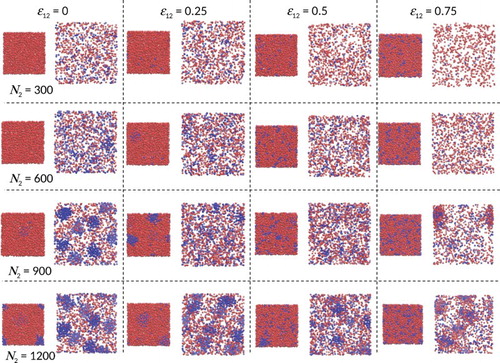
Figure 1 shows snapshots from these Gibbs-ensemble simulations at equilibrium. Only four types of phase are observed, with their existence dependent on the component densities and the strength of the cross-interaction; uniform vapour, uniform liquid, vapour with clusters and liquid with clusters. When , we find the following sequence of equilibrium behaviour as the concentration of SALR particles (component 2) increases: (i) vapour/liquid coexistence, (ii) vapour with clusters coexisting with uniform liquid, (iii) vapour with clusters coexisting with liquid with clusters. This shows the SALR clusters preferentially partition into the vapour phase when . When , the sequence is similar except the SALR clusters appear to preferentially partition into the liquid phase, i.e. the liquid phase with clusters has become more stable. The same sequence is observed for , except in this case, the CCC has increased, i.e. the uniform liquid has become more stable. When , we see qualitatively different behaviour in that the liquid no longer exhibits giant clusters at all, and giant SALR clusters apparent in the vapour phase are mixed and swollen with component 1 (the SA component).

Figure 1. Gibbs-ensemble MC simulation snapshots for SA/SALR binary mixtures having different cross-interaction strengths (see online version for colours).

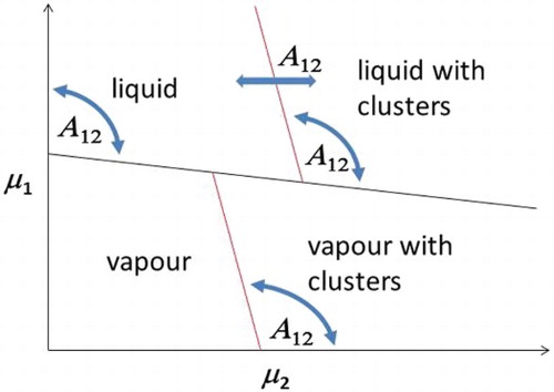
A tentative generic phase diagram for low SALR particle concentrations is sketched in Figure 2 based on these Gibbs-ensemble results. The usual vapour–liquid coexistence occurs when SALR particles are absent if (as is the case here) the SA system by itself is subcritical. Red lines denote the critical cluster chemical potential () of SALR particles in the vapour and liquid phases, assuming that the SA and LR interactions are balanced such that they lead to SALR clusters in the absence of component 1. The curved arrows indicate that the slopes of these critical cluster lines will depend on . Likewise, the horizontal arrow indicates the position of the liquid will vary with . For low and high values of , the Gibbs-ensemble simulation results suggest it will initiate to the right of the end of the vapour . But for intermediate values of , it can initiate to the left of the vapour . For sufficiently high values of , it appears from the simulations that clusters are no longer stable in the liquid phase. Of course, being a sketch, we have used straight lines, but we fully expect all the lines in this diagram to be curved in practice.

Figure 2. Tentative phase diagram for the binary SA/SALR mixture based on Gibbs MC simulations (see online version for colours).

While these simulations provide an indication of the equilibrium behaviour for the mixtures studied, a detailed exploration of the phase diagram quickly becomes time consuming. For every choice of the set of model parameters, many simulations are required to adequately explore the phase space in the cluster region and provide relevant averages for cluster sizes and compositions. Given that each simulation can take many hours, this situation is not ideal. Particularly as we wish to be able to make fast predictions of phase behaviour to assist in the design of nanoparticles synthesised via this giant SALR cluster route. Just as importantly, we cannot guarantee that these simulations are truly at equilibrium. This would require Monte Carlo moves that swapped clusters between simulation boxes.

We therefore developed a thermodynamic model, described next, for fast prediction of phase behaviour and to confirm the tentative phase behaviour shown in Figure 2.

4. Thermodynamic model

The thermodynamic model of Sweatman et al. [10], which was developed to investigate the cluster fluid phase of the one-component SALR fluid, is now extended to this binary mixture. The resulting model can be viewed as a kind of density functional micelle theory. An advantage of this particular approach is its basis in statistical thermodynamics and density functional theory, i.e. it relates the properties of constituent particles (the interaction model or Hamiltonian) to resulting phase behaviour, rather than taking emergent properties, such as the surface tension, as input to the model, as is more common in theories of clustering and micellization. The model is designed to treat each of the four phases seen in the simulations in Section 3.

As the one-component SALR thermodynamic model was described in detail in an earlier work [10], here we present only a summary of the binary model used in this work, stressing the key modifications for its extension to binary systems. The approach is based on the 'capillary model' approximation and treats the cluster fluid phase as a disordered collection of spherical liquid-like droplets of volume each, dispersed within a background vapour. Each cluster of particles (or droplet), with diameter , is taken to be identical with uniform body densities and for the two components, respectively, where and denote the number of particles of type 1 and 2, respectively, within each cluster. The cluster density is , where is the number of clusters within a system of total volume V, and the corresponding average background fluid densities are and , where and are the number of particles of each type in the background fluid.

Although, in general, clusters are polydisperse in their size and shape, they are statistically identical, and so in this model, they are chosen to be spherical and monodisperse. Therefore, the profile of a cluster centred at is, (6) where Θ is the Heaviside step-function. Thus, the 'capillary' model defines a discontinuous interface between the clusters and the background fluid. The volume fraction ψ of the clusters is, (7) where and are the total, or bulk, density of particles of type 1 and 2, respectively.

Unlike for the original derivation, where the model was presented using the Canonical ensemble (i.e. in terms of the Helmholtz free energy), for the binary mixture case, here we rewrite it in terms of the Grand-potential density, , (8) where is the chemical potential of component i. Following the original approach by Sweatman et al. [10], the free energy contributions are split into two contributions: energetic contributions coming from pair interactions, and entropic contributions obtained by treating particles and clusters as hard spheres. The Helmholtz free energy () can also be partitioned into 'self' and 'mixture' contributions, (9) In this equation, describes the free energy density of particles within clusters, while contains contributions to the free energy density of the mixture from both the background fluid and the clusters. Simple expressions for and are now developed in terms of the basic parameters describing particle interactions. At all times, we only consider the configurational contribution to the free energy, as the contribution from momentum (involving the thermal de Broglie wavelength) is unimportant for equilibrium behaviour.

4.1. Self-free energy

The self-free energy of the clusters is composed of two terms, (10) In Equation (10(10) ), is the interaction energy between particles in a cluster, i.e. its self-energy, and is the entropy of the particles within a cluster. To estimate , we assume configurational correlations between particles within a cluster are similar to those within a bulk liquid. So the interaction energy of particles within a cluster is given by, (11) where is the radial distribution function (RDF) between particles i and j in a bulk liquid, and is related to the form factor of the clusters and represents the geometric convolution of two cluster distributions. The liquid RDFs are approximated by those of a hard sphere fluid, (12) where the Percus–Yevick (PY) theory [12] for hard spheres at the combined liquid density is used.

The self-entropy is approximated as, (13) where is the entropy density of a uniform hard sphere fluid mixture of components with densities and , respectively, and is the cluster interfacial area.

Unlike in the original model derivation [10], the model now also takes into account the entropic contribution of the primary particles at the interface between the background fluid and the clusters, represented by the right-most term in Equation  (13(13) ). Assuming a planar step-like density profile at the interface, the interfacial entropy density is (14) The excess free energy density for the gas–liquid interface is calculated using the Rosenfeld et al. [13] fundamental measure functional (FMF) for hard spheres, (15) and the uniform background fluid, , and cluster liquid, , hard sphere excess free energy densities are calculated from the same in the limit of a bulk fluid mixture.

In Equation (15(15) ), there are only three independent parameters, , and , which are calculated in the planar limit through, (16) where the independent parameters are calculated using the following weight functions of the Rosenfeld functional, (17) (18) (19) The remaining scalar weight functions are proportional to , and the remaining vector weight function is collinear with as indicated by Rosenfeld [13], (20) (21) (22) Finally, the local densities for each component, , on either side of the interface take on the values inside the cluster for , and in the background fluid for x>0.

4.2. Mixing free energy

We deal with the contribution of the energy density to the mixture free energy first, which is given exactly by the usual energy equation [14], (23) where is the RDF between particles i and j in the background fluid, is the RDF between component i in the background fluid phase and cluster centres, and is the cluster center-cluster center RDF. Also, is the effective pair-potential between component i in the background fluid phase and cluster centers, and is the effective pair-potential between cluster centers.

Convenient approximations for all these functioare made as follows [10] (24) (25) (26) where the combined vapour density is . Here it is assumed that no particle can approach a cluster (that it is not part of) closer than , since then it would be considered part of that cluster. These cluster-cluster and cluster-vapour approximations are adequate for this work. In any case, more accurate approximations are not obviously available, since integral equation approaches to this problem of giant SALR clustering typically fail in the low-density region of the SALR phase diagram in which we are interested.

The effective interactions are computed in k-space as, (27) (28) The entropy of the coarse-grained system, due to these effective interactions, is approximated in terms of a hard sphere mixture with significant negative non-additivity (see Sweatman et al. [10] for a discussion on this). As there is no satisfactory existing expression for the entropy of such a system, the background fluid and cluster excess entropies are decoupled, (29) where is the effective cluster diameter calculated via the Barker-Henderson prescription [14], (30) which also defines an effective packing fraction of clusters, (31) Again, we use Rosenfeld's FMF [13], which reduces to the PY compressibility result [14] for a bulk fluid, to calculate the excess hard-sphere free energy density.

The ideal gas contribution in Equation (29(29) ), omitting terms involving the thermal de Broglie wavelength of the primary particles, is simply, (32) The term in Equation (29(29) ) is a centre-of-mass correction, which ensures the coarse-grained clusters have a precisely defined position (again, see Sweatman et al. [10] for a discussion on this point) and can be seen as contributing to the entropy of formation for the clusters. For this contribution, we used an appropriately modified version of our previously derived expression [10] for the pure SALR system, (33) In Equation (33(33) ), choosing gives the same expression derived originally for the pure SALR fluid in earlier work. For the binary system in this work, we found for low cluster body densities () that the formation of unrealistically small clusters with less than four particles was sometimes favoured due to an under estimation of the cluster formation entropy (i.e. the contribution) which cannot adequately compensate the ideal-gas cluster contribution , which favours the formation of clusters. This problem arises because of an error in the derivation of this term in [10]. Indeed, it is in principle impossible to specify the formation free energy of a cluster precisely without first specifying how a cluster is defined, i.e. specifying the rules that govern when a particle is considered part of a cluster. As we do not specify those rules here, we cannot in principle exactly formulate an expression for . 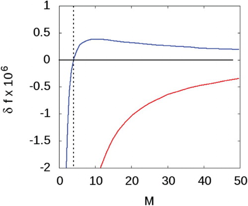Viewed another way, the final term on the right hand side of (33(33) ) is arbitrary, and only determined precisely when a rule governing the definition of a cluster is imposed. As we do not do this here, we must regard this final term as an adjustable parameter. Thus, we adjust α to ensure that the smallest cluster is comprised of at least four particles. The parameter that satisfies this condition, and therefore the one used in the remainder of this work is (see Figure 3).

Figure 3. versus the total number of particles in the cluster for the low liquid density . Red line using with , and blue line with . The point at M=4 when is marked with a vertical dashed line (see online version for colours).

This completely defines the thermodynamic model for the cluster fluid phases of the binary mixture. For a uniform fluid without clusters, the free energy is expressed simply as, (34) where .

4.3. Cluster solid model

For sufficiently high SALR chemical potentials, a cluster solid phase is expected [10]. A thermodynamic model of the cluster solid phase was not included in the earlier one-component model; instead a criterion based on the effective packing fraction of clusters, , was used to locate this phase boundary [10]. In the present work, we instead prefer to maintain a thermodynamicapproach, and thus develop a thermodynamic model of the cluster solid phase.

First we introduce the relative packing fraction, z, which is related to the effective packing fraction and is calculated as follows, (35) with 0<z<1.

When considering the crystal packing of solid spheres, there are two main staking arrangements that are favoured: face-centred-cubic (fcc), and hexagonal-closed-packed (hcp), since they both provide the most efficient packing (occupying about of the space). These two structures have been the focus of many studies, with Sion-Chuon and Huse [15] reporting that the fcc stacking has the highest entropy. We therefore proceed to model the cluster solid phase of our binary system as an fcc solid.

In order to account for the cluster solid phase, the thermodynamic model requires two modifications. First, the cluster-cluster RDF in Equation (26(26) ), , which is suitable for a cluster fluid, must be replaced with a suitable RDF for the fcc cluster solid. For computational efficiency, we use an empirical fit to the hard sphere fcc crystal RDF developed by Choi and Ree [16] valid for separations up to provided 0.700<z<0.985. For larger separations, we take .

Second, the entropy density of clusters, which for the cluster fluid phase is given by the term in Equation (29(29) ), must be modified to account for the fcc crystal phase. We use an empirical equation proposed by Speedy [17], (36) with the fcc parameters being: a=0.5921, b=0.7072, c=0.601 and . This expression provides the excess entropy per hard sphere at a packing fraction z and is valid for 0.643<z<0.990. To employ this equation of state for our fcc phase of clusters, we use the relative packing fraction (Equation 35(35) ) and multiply by to obtain a reduced excess free energy density. As our main interest here is to locate the cluster fluid to cluster solid phase transition, we are not interested in cluster solid phases with high packing fractions and so impose the constraint z<0.9.

4.4. Solving the model

Minimisation of the grand-potential density with respect to the primary variables (i.e. the vapour densities , the cluster body densities , the cluster size and the cluster volume fraction ψ at fixed chemical potentials () with a defined set of interaction strengths is performed via a local down-hill search algorithm. Phase space is searched on a square grid of chemical potentials. For each grid point, we compare the grand free energy densities calculated for uniform fluid, cluster fluid and cluster solid, taking the lowest free energy as the equilibrium phase. We impose the constraint M>4 consistent with Figure 3.

In what follows we present our results in terms of reduced fugacities rather than chemical potentials, where the reduced fugacity can be readily obtained from the configurational part of the chemical potential as . This reduced fugacity equals the packing fraction of hard spheres in the dilute limit.

5. Results and discussion

5.1. Thermodynamic model validation

While the thermodynamic model was developed for binary mixtures, it should also reproduce the phase behaviour of the limiting cases: i.e. the pure SA fluid and the pure SALR fluid. The model is forced to mimic the respective pure fluid by setting the chemical potential of the other component to an arbitrarily low number.

The SA fluid phase diagram is presented in Figure 4. When the attractive parameter is very low (equivalent to high temperatures), the fluid shows supercritical behaviour. As increases (equivalent to decreasing the temperature in the system), the fluid reaches a critical point at about eventually showing the typical first-order gas–liquid phase transition with fugacity, as expected for this system (Figure 4(b)).

Figure 4. Phase diagram for the pure SA fluid with , over a range of attractive strengths, . (a) Phase map showing vapour and liquid regions, (b) 3D plot clearly showing the first-order vapour–liquid transition. The location of the critical point is highlighted in black, while the location of the sub-critical phase change at is highlighted in red (see online version for colours).

Results for the predicted phase diagram of a pure SALR fluid with and , identical to the parameters used originally by Sweatman et al. [10], are presented in Figure 5, in which the cluster-fluid phase is shown in red and the cluster solid phase in blue. These results were obtained by sweeping in 0.025 intervals, and in intervals, and they agree well with those presented by Sweatman et al. [10].

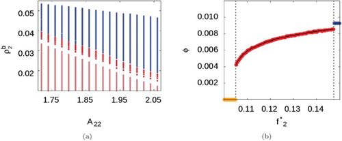
Figure 5. Phase diagram for the pure SALR fluid with , , and . (a) Phase map when , showing the uniform phase (salmon), the cluster fluid phase (red), and the cluster solid phase (blue). (b) Transitions (black dotted lines) observed at : uniform phase (orange) to cluster fluid (red), to cluster solid (blue). (see online version for colours)

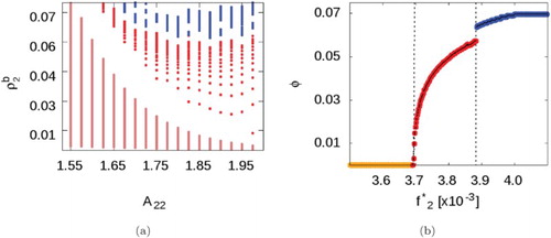
Figure 5(b) shows results specifically for studied by changing the chemical potential in small intervals of . As expected, increasing fugacity leads to the appearance of a cluster-fluid phase. Further increasing fugacity results in increased volume fractions until, at high fugacities (i.e. high SALR concentrations), there is evidence of a discontinuous cluster-fluid to cluster solid phase transition.

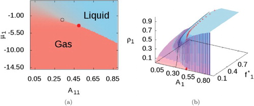
We then proceed to map the phase diagram for an SALR fluid with parameters identical to those used in the Monte Carlo simulations shown in and which form the focus of this present work, i.e. with a longer-ranged repulsive interaction, . Figure 6(a) shows results obtained by incrementing in intervals of 0.02 and in intervals of . Although the cluster-fluid phase now exists over a wider range of fugacities, these correspond to a smaller range of bulk densities. As in the previous SALR system, at high fugacities, there is a discontinuous phase change from cluster-fluid to cluster solid, but now there is also a first-order phase transition between the uniform and cluster-fluid phases.

Figure 6. Phase diagram for the pure SALR fluid with , , and . (a) Phase map when , showing the uniform phase (salmon), the cluster fluid phase (red), and the cluster solid phase (blue). (b) Phase transitions (black dotted lines) observed at : uniform phase (orange) to cluster fluid (red), to cluster solid (blue). (see online version for colours)

5.2. Binary mixtures

From here on the discussion will focus on SA+SALR binary mixtures. In particular, two different cases will be discussed: supercritical SA fluid (represented in an ideal sense using hard spheres, ), and a subcritical SA fluid (). A summary of the relevant parameters in both cases is presented in Table 1. We then investigate the effect of changing the strength of the cross-interaction strength () in each case.

Table 1. Parameters for the binary mixtures studied.

Mixture
I	0.00	1.85	0.50	1.00	0.25
II	0.50	1.85	0.50	1.00	0.25

Note: The cross-interaction parameter is within the range .

Unlike the pure fluid case, model solutions for binary systems require more computational effort, as each specific grid point on the , phase diagram involves a complex multi-variable global minimisation, which is susceptible to the initial conditions chosen. For this reason, our final phase diagrams for the binary mixtures are found by comparing four different sets of solutions obtained by sweeping the phase space up/down on each chemical potential. Phase diagrams are conveniently viewed in terms of the cluster volume fraction, φ.

5.3. Mixture I

We initially consider this mixture (parameters in Table 1) for the case where , modelling an SALR fluid containing inert impurities. The phase diagram obtained (Figure 7(a)) shows that for very low SA fugacities the uniform to cluster-fluid phase transition approaches the pure SALR fluid case. However, despite the absence of a cross-interaction, as the SA concentration increases (i.e. increased fugacity) Figure 7(a) shows higher SALR fugacities are needed to achieve the cluster-fluid phase, i.e. the presence of an inert impurity delays clustering, but with no significant effect on the cluster size or the cluster volume fraction at the transition to a cluster solid (Figure 7(b)).

Figure 7. Mixture I with parameters given in Table 1 and . (a) Volume fraction phase diagram, where the green line highlights (i.e. ). (b) Cluster size. (c) Total phase density (blue) and compositions (red) when . Background fluids represented by dotted lines, while cluster phases represented by solid lines. A dashed black line marks the appearance of the cluster fluid phase, while the dashed green line marks the cluster-fluid to cluster solid transition (see online version for colours).

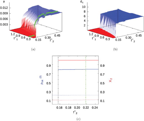
Figure 7(c) shows the density and composition of background fluid and clusters for a fixed SA fugacity (i.e. ). The background fluid is formed mainly of SA particles at low concentration, while clusters are almost pure SALR with liquid-like density. As the SALR fugacity is increased, we see first-order phase transitions from the uniform fluid to the cluster fluid, and finally to the cluster solid.

The model shows some uncertainty in the cluster solid region, where it often alternates between two solutions, one depicting slightly smaller (by ), denser (by ) clusters with lower volume fractions (by ). This is likely an artefact of our model for the cluster solid phase, which assumes monodisperse clusters, and/or due to the solution method which is not guaranteed to find the global minimum of the free energy.

5.3.1. Mixture I: increasing

Mixture I as presented so far may be relevant for systems with inert impurities. However, real mixtures will always have some degree of cross-interaction (), the nature of which plays a key role in the phase behaviour of the system.

As the cross-interaction strength is increased, the behaviour remains similar to that presented in Figure 7, except for the composition of the background fluid, which presents a higher amount of SALR particles at lower overall density.

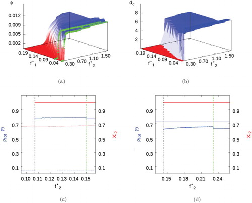
Figure 8 shows the result of increasing the cross-interaction to . Qualitatively different be-haviour is now observed. The transition to the cluster fluid phase is no longer delayed by the SA fluid, rather it is promoted by it: notice the uniform to cluster-fluid transition line moves towards the left (i.e. towards smaller SALR fugacities) as the SA fugacity increases (Figure 8(a)). Both the background phase and clusters have a significant proportion of SA and SALR particles, due to the increased SA–SALR inter-particle affinity. In turn, this causes an increase in the cluster size relative to weaker cross-interactions, which then leads to a reduction in the density of clusters.

Figure 8. Mixture I with parameters given in Table 1 and . (a) Volume fraction phase diagram, green lines highlight and 0.039 (i.e. and ). (b) Cluster size. (c) and (d) Total phase density (blue) and compositions (red) when and 0.039. Uniform/background fluids represented by dotted lines, while cluster phases represented by smooth lines. A dashed black line marks the appearance of the heterogeneous cluster phase, while the dashed green line marks the cluster-fluid to cluster solid transition (see online version for colours).

5.4. Mixture II

In this case, the SA fluid is subcritical, thus allowing us to explore the effect of a second component with strong attractive interactions when mixed with the SALR fluid of interest. As before, we first study the case without cross-interactions . Comparing Figures 7 and 9, although we see the same sequence of transitions, from uniform fluid to cluster-fluid to cluster solid, there is a noticeable change in phase behaviour, with respect to Mixture I, when the background fluid condenses.

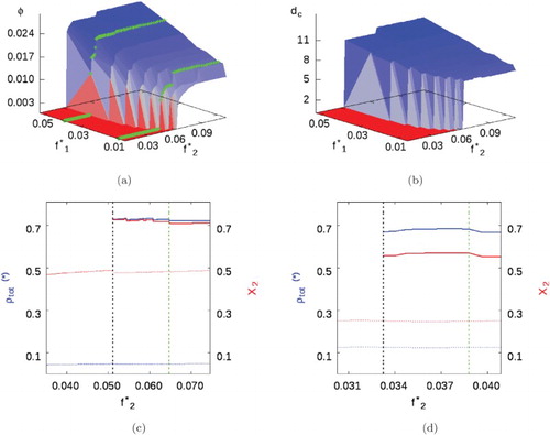
Figure 9. Mixture II with parameters given in Table 1 and . (a) Volume fraction phase diagram where green lines show and 0.039 (i.e. and ). (b) Cluster size. (c) and (d) Total phase density (blue) and compositions (red) when and 0.039. Uniform/background fluids represented by dotted lines, while cluster phases represented by smooth lines. A dashed black line marks the appearance of the heterogeneous cluster phase, while the dashed green line marks the cluster-fluid to cluster solid transition (see online version for colours).

For low SA fugacities, the uniform phase being a low-density vapour (Figure 9(c)), the system behaves almost as a pure SALR fluid, as expected, except with some SA particles in the background fluid. However, at high SA fluid fugacities, when the background phase is liquid-like (Figure 9(d)), the SALR fugacity required for clustering increases almost linearly with increasing SA fugacity (and hence with SA density). In this regime, clusters are almost pure SALR, while the background fluid is nearly pure SA.

5.4.1. Mixture II: increasing

Slightly increasing the cross-interaction () shows no significant change in the shape of the phase diagram, but with the noticeable difference that the critical cluster fugacity (CCf) at the liquid-like and vapour-like homogeneous phases no longer intersect. This is because the CCf in the liquid-like background phase, though still almost linearly dependent on , has been pushed back to higher SALR fugacities, indicating in this case, the cluster fluid is less stable when the background fluid is liquid-like.

As the cross-interaction increases, i.e. to (Figure 10(a)), the transition from vapour to liquid occurs at smaller SA fluid fugacities and for sufficiently low , the system behaves almost like a pure SALR fluid. But as the SA fugacity increases, clustering occurs at lower SALR fugacities, just as for the case with a supercritical SA component (Mixture I). These clusters have diameter similar to the earlier cases, with .

Figure 10. Mixture II with parameters given in Table 1 and . (a) Volume fraction phase diagram, the green line highlights (i.e. ). (b) Cluster size. (c)Total phase density (blue) and compositions (red) when . Uniform/background fluids represented by dotted lines, while cluster phases represented by smooth lines. A dashed black line marks the appearance of the heterogeneous cluster phase, while the dashed green line marks the cluster-fluid to cluster solid transition (see online version for colours).

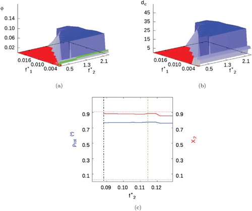
But, in the region of the phase diagram where the background fluid condenses, where the fugacity of the SA fluid is sufficiently high, the model generates some unexpected results. Under these conditions, the model predicts the formation of giant clusters () with a low body density, not very different to the background phase. In other words, a very weakly modulated phase is formed. It is not clear if this is the correct behaviour or an artefact of the thermodynamic model. This can be further investigated by the use of a mean-field non-local DFT, but this is beyond the scope of the present work.

6. Conclusions

We developed a thermodynamic model to study the equilibrium phase behaviour of a model SA+SALR binary fluid. Our multiscale DFT approach generates results consistent with those obtained from Gibbs-ensemble MC simulations for the same model mixture.

The DFT results support the MC simulation results in qualitative terms, and therefore the phase diagram sketched in Figure 2 appears to show the correct trends, even for the supercritical case where there is no bulk vapour–liquid phase transition. In particular, we find the cross-interaction largely determines phase behaviour. Its strength has a direct effect on the direction of the uniform fluid–cluster fluid phase boundary, which for low cross-interaction strengths moves towards higher SALR fugacities as the SA fugacity increases, while for high cross-interaction strengths moves towards lower SALR fugacities as the SA fugacity is increased. In other words, for low cross-interaction strengths, the presence of the SA component tends to delay cluster formation, while the opposite is true for strong cross-interactions.

Moreover, giant clusters can form readily, even if they would not form for the SALR component alone, provided the SA component concentration is sufficiently high and the cross-interaction is sufficiently strong. The SA composition within the clusters is significantly increased with increasing cross-interaction strength, with clusters swollen by the absorption of SA particles.

A useful way to consider the effect of the SA component is in terms of an additional effective interaction between SALR particles. If the cross-interaction is only weakly attractive, then the SA component induces a weak effective repulsion between SALR particles. But if the cross-interaction is strongly attractive, then SA particles induce an effective attraction between SALR particles. In each case, the strength of the effect is sensitive to the concentration (or chemical potential) of SA particles. We expect it might be possible to formalise this observation by integrating-out the SA component to generate an effective one-component SALR system.

This observation is very important for understanding the appearance of these kinds of giant cluster in experiments. Even though charged solutes might, by themselves, not form clusters under experimental conditions, when in the presence of an uncharged solute, which could be a different species of the same solute, clusters can still appear if the cross-interaction between them is strong enough. Essentially, it can happen that the uncharged species tends to 'glue' the charged species together. A giant cluster will still form if the screened coulomb repulsion of the charged species is sufficiently strong, such that formation of the bulk liquid phase is frustrated.

To our knowledge, this is the first theoretical approach capable of investigating both a disordered cluster phase (the cluster fluid) and a modulated phase (the cluster solid). It can also investigate the effect of the addition of a simple fluid component (i.e. the SA particles) on the clustering behaviour of an SALR system. By enabling the consistent treatment of a cluster solid phase on the same footing as the cluster fluid, we observe a first-order cluster fluid to solid transition for sufficiently high particle concentrations (or chemical potentials). In some cases, the model predicts the emergence of a very weakly modulated phase with very long wavelength fluctuations. It is not clear at this stage whether this is an artefact, and therefore a failure, of the model, or whether this behaviour is correctly predicted. Investigation of this feature can be tackled with a standard non-local DFT treatment.

More generally, the model opens the door to investigating giant cluster formation in experiments with multiple solute components, exemplified by soft matter and biological systems.

Disclosure statement

No potential conflict of interest was reported by the authors.

Additional information

Funding

The authors thank the Engineering and Physical Sciences Research Council (EPSRC) for generous funding as part of the SynBIM research collaboration [EP/P007236/1].

References

- F. Bordi, C. Cametti, S. Sennato, and M. Diociaiuti, Biophys. J. 91, 1513 (2006). doi: 10.1529/biophysj.106.085142
- A. Stradner, H. Sedgwick, F. Cardinaux, W.C.K. Poon, S.U. Egelhaaf, and P. Schurtenberger, Nature 432, 492 (2004). doi: 10.1038/nature03109
- L.A. Rodríguez-Guadarrama, S.K. Talsania, K.K. Mohanti, and R. Rajagopalan, Langmuir 15, 437 (1999). doi: 10.1021/la9806597
- A. Jawor-Baczynska, J. Sefcik, and B.D. Moore, Cryst. Growth Des. 13, 470 (2012). doi: 10.1021/cg300150u
- S. Chattopadhyay, D. Erdemir, J.M.B. Evans, J. Ilavsky, H. Amenitsch, C.U. Segre, and A.S. Myerson, Cryst. Growth Des. 5, 523 (2005). doi: 10.1021/cg0497344
- A.E.S. Van Driessche, M. Kellermeier, L.G. Benning, and D. Gebauer, New Perspectives on Mineral Nucleation and Growth (Springer, Cham, 2017).
- M.R. Ward, S.W. Botchway, A.D. Ward, and A.J. Alexander, Faraday Discuss. 167, 441 (2013). doi: 10.1039/c3fd00089c
- A.J. Archer and N.B. Wilding, Phys. Rev. E 76, 031501 (2007). doi: 10.1103/PhysRevE.76.031501
- A.J. Archer, C. Ionescu, D. Pini, and L. Reatto, J. Phys. Condens. Matter 20, 415106 (2008). doi: 10.1088/0953-8984/20/41/415106
- M.B. Sweatman, R. Fartaria, and L. Lue, J. Chem. Phys. 140, 12450812451124508–1 (2014). doi: 10.1063/1.4869109
- M.B. Sweatman and L. Lue, J. Chem. Phys. 144, 17110217111171102–1 (2016). doi: 10.1063/1.4948784
- Y. Rosenfeld, Phys. Rev. Lett. 63, 980 (1989). doi: 10.1103/PhysRevLett.63.980
- Y. Rosenfeld, M. Schmidt, H. Löwen, and P. Tarazona, Phy. Rev. E 55, 4245 (1997). doi: 10.1103/PhysRevE.55.4245
- J.P. Hansen and I.R. McDonald, Theory of Simple Liquids, 2nd ed. (Academic Press, London, 1986).
- M. Siun-Chuon and D.A. Huse, Phys. Rev. E 59, 4396 (1999). doi: 10.1103/PhysRevE.59.4396
- Y. Choi and T. Ree, J. Chem. Phys. 95, 7548 (1991). doi: 10.1063/1.461381
- R.J. Speedy, J. Phys. 10, 4387 (1998).