Ring polymers are much stronger depleting agents than linear ones

ABSTRACT

We investigate the conformations and shapes of circular polymers close to planar, hard walls as well as the ensuing ring–wall and polymer-induced wall–wall interactions in ring polymer solutions. We derive, by means of Monte Carlo simulations, the effective interaction potential between the centres of mass of flexible, unknotted ring polymers and a hard wall for different polymerisation degrees N. Adopting the coarse-grained description of ring polymers as ultrasoft, penetrable spheres, mean-field density functional theory is then employed in order to examine ring polymer solutions under confinement. We demonstrate that, below the semi-dilute regime, ring polymers structure close to walls much more strongly than their linear counterparts, their density profiles featuring pronounced oscillations. Moreover, the polymer-induced depletion potential between the two walls exhibits an oscillatory profile reminiscent of hard-sphere systems, with oscillations that intensify upon increasing polymer concentration. The obtained form of the depletion interaction is shown to be qualitatively different in comparison to the case of linear polymer solutions at the corresponding densities.

GRAPHICAL ABSTRACT

KEYWORDS:

• Ring polymers
• coarse-graining
• density functional theory
• confinement
• depletion

1. Introduction

Solutions and melts of ring polymers represent a class of macromolecular systems whose structural and dynamical properties in and out of thermodynamic equilibrium are profoundly influenced by the polymers' topological constraints. At the single-molecule level, these restrictions were formulated decades ago in terms of an additional topological interaction that arises between two closed polymeric chains which are not allowed to concatenate. Surprisingly, this interaction leads to an effective repulsion between the rings even in the case of absent excluded volume interactions [1,2]. Macroscopically, the topological effect brings about a series of major differences between chemically identical ring and linear polymers of the same length including, for example, a distinct θ-point of ring polymers in solution [3,4] and an unusual power-law stress relaxation of entangled ring polymer melts [5]. Further, topological constraints have a great relevance in biological systems: from viral capsids [6–9] to kinetoplast [10–12] and chromosomes in eukaryotes [13–15], topology plays a crucial role, for example, influencing and, in some cases, enhancing the organisation and the stability of chromosomes.

Over the past years, coarse-graining methods have emerged as powerful and computationally accessible tools for studying mesoscopic soft-matter systems. They hinge on the fact that the intrinsically many-body interaction between two polymers can be reduced to only a few coupled degrees of freedom, such as their centre of mass coordinates, canonically tracing out the fine-grained degrees of freedom and therefore leaving its thermodynamic properties preserved [16,17]. Within such description, solutions of polymers can be represented as effective fluids composed of penetrable particles that interact via some effective, ultrasoft pair potential, . The same strategy can be put into practice in the case of interactions between polymers with different topology or polymers and colloidal particles, leading to a complete, multi-scale effective picture of such mixtures. In particular, this approach has been successfully applied to the description of linear [18–22], ring [4,23–31] and star [32–34] polymers, block copolymers [35,36], dendrimers [37] and polymer nanocomposites [38–42].

In the case of fully flexible ring polymers in good solvent, off-lattice simulations have revealed that the effective interaction possesses a drastically different form in comparison to linear chains [23,24], which in the latter case is Gaussian as confirmed by numerous computational and theoretical approaches [21,23,35,43,44]. In particular, for the simplest case of an unknotted (also, the so-called -knot) ring polymer, it exhibits a plateau at about in the region for , where denotes the gyration radius of a free polymer. On the contrary, shorter rings feature higher amplitudes of the potential with a minimum at r=0. Further studies have shown that the potential between the centres of mass of two rings depends additionally on the knottiness of two interacting polymers (e.g. , , ) and their polymerisation degree [26]; nevertheless, the effective potentials between all closed polymers seem to converge towards a universal, master curve obtained previously for the -topology in the limit of very long macromolecules.

The origin of the plateau of the effective potential between rings at close separations can be understood by considering the mechanism of how the centres of mass of the rings approach each other: one polymer expands, whilst the other shrinks and gets nested within the former. These observations allowed to formulate a simple but accurate theory of ring–ring interaction, in which the coils are modelled as two unequal-sized, soft spheres [25]. The very distinctive form of this effective potential implies that the structure of confined ring polymer solutions and, especially, depletion interactions between hard objects, such as colloids or hard walls, mediated by them may have a very different form in comparison to the case of linear chains. The possible dissimilarity would originate purely from the non-trivial topological state of a ring obtained by joining the ends of a chemically identical, linear polymer together.

The study of depletion interactions has a great practical relevance in a wide range of applications as it affects the stability of polymeric and colloidal suspensions [45]. Essential in understanding these interactions are two ingredients: first, the aforementioned interactions between the depletants and second, the interactions of the depletants with the solid obstacles (walls or colloids). For depleting agents with internal, fluctuating degrees of freedom, such as polymers of any architecture or topology, a careful coarse-graining approach is necessary, since the ways in which an obstacle reduces the entropy of a neighbouring polymer strongly depend on the polymer itself. A quantitative measure of the depletion between two objects is provided by the depletion potential effectively acting between the large particles after thermodynamically integrating out the smaller ones [16]. Our final attention in this article will be drawn precisely to the depletion interaction between two hard walls immersed in a solution of ring polymers and its distinction compared to the case of linear ones. Going beyond the Asakura–Oosawa model, which predicts an exclusively attractive form of the potential between the walls [46–48], we employ a mean-field theoretical approach, taking into account additional correlations between interacting coils [18,19]. These correlations are much more pronounced in the case of hard, spherical depletants, which in the latter case result in an oscillating profile of the potential [16]. We find that, surprisingly as it seems at first sight, the ring-induced depletion interaction is much more similar to that induced by hard spheres than to that induced by linear polymer chains. Interestingly, such a difference cannot be traced back to the limit of stiff linear and ring polymers, corresponding to hard rods and disks, respectively: in both cases the rod- and disk-induced depletion potentials between two colloids feature a similar form with a repulsive maximum at about for comparable, dilute concentrations of the depletants [49–51].

The rest of the article is structured as follows: after providing an overview of the employed computational and theoretical methods in Section 2, we briefly consider in Section 3.1 the effect of slit-like confinement on the metric properties of a flexible, unknotted ring. In Section 3.2, these results are compared to the case of a single-wall confinement, when the shape, size and orientation of the polymer are investigated in dependence on the separation between its centre of mass and a planar, impenetrable wall. These two sections serve as a bridge between properties of confined ring polymers at a single-molecular level and in solution, which are discussed afterwards. In Section 4, we supplement the above-mentioned, coarse-grained model of ring polymers with an effective interaction potential between the centres of mass of the polymer coils and a hard wall obtained by means of Monte Carlo (MC) simulations. The effective potentials are then used in Sections 5 and 6 to obtain the equilibrium structure of confined ring polymer solutions employing standard density functional theory (DFT) methods within the range of applicability of the effective model, that is, in the dilute concentration regime. In order to characterise ring polymers as depleting agents, in Section 6 we present the depletion potential acting between two plates immersed in the solution thereof, which, as we will show, possesses an oscillating profile that intensifies with increasing density of the fluid. Moreover, to show a clear difference between confined ring and linear polymer solutions, we systematically compare the results that can be obtained for the two aforementioned architectures using effective models. Finally, we summarise and conclude in Section 7.

2. Model and methods

We briefly consider in this section the theoretical and numerical methods used throughout the article. In particular, we first present details on the MC numerical simulations, then we define the metric properties for a ring polymer. Finally, we give a concise introduction to the employed DFT calculations.

2.1. Numerical simulations

We perform off-lattice MC simulations of fully flexible, unknotted ring polymers to investigate their metric properties under planar confinement and to develop an effective, coarse-grained model for the interaction between their centres of mass and a planar, impenetrable wall. The system is always at the so-called infinitely dilute concentration, i.e. we consider only one ring confined by one or two hard walls.

Polymer chains are modelled using a standard, bead-spring model, introduced by Grest and Kremer [52]. The excluded volume interactions among the beads are modelled by the Weeks–Chandler–Andersen (WCA) potential (1) where denotes the Heaviside step function. The potential is purely repulsive and therefore resembles good solvent conditions. Neighbouring monomers along the backbone are bound with the finitely extensible nonlinear elastic (FENE) potential (2) where we choose .

Unless otherwise stated explicitly, hard walls in our simulations are parallel to the xy-plane of a Cartesian coordinate system, and act as additional external potentials for all the monomers. The functional form for the interaction between the hard walls and the monomers is chosen to be (3) where denotes the position of a bead. Such a choice is suitable for MC simulations. If only one wall is considered, it is placed at z=0 and fills the region with ; otherwise, a slit of width d is obtained as a superposition . Finally, we choose σ as our unit of length and set the reduced temperature to unity .

Metropolis MC simulations are performed employing simple translational displacements of individual monomers in conjunction with collective crankshaft moves; one MC step is defined as a combination of N trial translational moves and one crankshaft move. During a crankshaft move for a polymer (either ring or linear) with N beads, we randomly choose two of its monomers that are separated by at most N/3 particles and rotate the shorter of the two formed segments by a random angle around the axis connecting the two chosen monomers (for further details, see appendix A of [27]). Relevant quantities were usually sampled every  MC steps, which corresponds to a complete decorrelation of configurations for the longest polymer considered in weak confinement (decorrelation times for strong confinement, i.e. close to hard walls, are typically higher by two orders of magnitude).

Special attention must be paid to the topological state of a ring polymer, which has to be preserved. Therefore, we strictly forbid any violation of the initial topology of the ring by rejecting every trial MC move for which a bond crossing had occurred, employing the algorithm outlined in appendix A of [25]. On the other hand, topology does not constrain phase space exploration for linear polymers and thus checks for bond crossings are not included in simulations of linear chains.

Further, we shortly discuss the method employed for calculating the effective potential between the centre of mass of a polymer and a planar, hard wall located at z=0. In this case, will depend solely on z, as the translational symmetry of our system is broken in the z-direction only due to the presence of external field . More precisely, can be defined as follows [16]: (4) where stands for the probability density of finding the centre of mass of the polymer at a distance z away from the wall, whereas the term accounts for the normalisation of the effective potential: . Accordingly, we employ a standard umbrella sampling technique [53] to measure the distribution function : the whole region of interest is divided into ‘windows’ of width centred at (), within which the effective potential does not vary more than few . It is important to note that the neighbouring windows must overlap, so that the effective potentials sampled in separate windows could be joined afterwards. Furthermore, an additional local bias potential has to be included to assure that the polymer remains within the preset region of space. In particular, in our MC simulations we used an infinite well bias potential, which diverges as the centre of mass of the polymer crosses the boundaries of the current sampling window, and vanishes otherwise. As a result, can be obtained from the distribution functions , which yield the probability density of finding the centre of mass of the polymer in the jth window at a distance z away from the wall, as follows: (5) where 's are needed to join together the potentials in neighbouring windows, and they have been determined as described in  [54].

2.2. Metric properties

The shape, size and orientation of a macromolecule, often named metric properties, can be described with the help of the eigenvalues and eigenvectors of its radius of gyration tensor G [55], whose components are given by the following expression: (6) where 's denote the coordinates of each constituent part of the molecule, is the position of its centre of mass and the indices α and β () stand for the three Cartesian components.

More specifically, let us assume that , and are the three eigenvalues of the matrix G in Equation (6(6) ) sorted in the descending order (i.e. ) and the associated normalised eigenvectors are and . Then, the average size of a polymer is given by the root-mean-square value of the gyration radius with . In order to describe its average extension in the directions parallel and perpendicular to the walls, we use the root-mean-square values and , respectively, defined as follows: (7a) (7b) where denotes the angle between the eigenvector and the z-axis such that .

Finally, alignment of the eigenvectors along the out-of-plane (z) direction can be conveniently quantified by means of the second Legendre polynomial (8) which averages out to 0, if there is no preferred orientation for along . Furthermore, a value of 1 or indicates that is predominantly aligned in the direction of or orthogonal to it, respectively.

2.3. Density functional theory

DFT represents a powerful tool for studying classical inhomogeneous systems that typically encounter in fluid theory and soft matter [56]. It hinges on two fundamental theorems [57–59] stating that the grand potential Ω of a system subject to an external potential in the grand canonical ensemble is a unique functional of the equilibrium single-particle density . Accordingly, can be obtained by minimising the grand potential functional (9) with respect to . Here, denotes the fixed value of the chemical potential of the fluid, and the ideal free energy functional is given by the well-known expression (10) where and . The excess free energy term is generally unknown and quality of results heavily depends on the approximations made. In this work, we model it using the mean-field functional (11) which has been proven to deliver accurate results for ultrasoft pair potentials [60–65] (i.e. those satisfying the integrability condition in three dimensions). In particular, the effective, coarse-grained interaction between two ring polymers [24–26], as well as between two linear chains [16,18], belongs to this class of potentials.

Application of the minimisation principle to grand potential functional (9(9) ) yields the following integral equation for the equilibrium density profile: (12) Furthermore, for the sake of convenience, μ in the equation above can be replaced with the bulk density of the fluid, , by taking into account the free energy of the bulk fluid in our model (13) where . Note that the constant is finite due to integrability of the potentials considered. Consequently, Equation (13(13) ) implies that (14) Therefore, original integral equation (12(12) ) can be recast in terms of the bulk density as follows: (15) In Sections 5 and 6, we will present the numerical solution of Equation (15(15) ) for ring polymers under confinement, combining the well-known effective interaction between rings [24–26] with the effective interaction between the ring polymers and the hard wall, reported in Section 4.

3. Metric properties of a ring polymer under confinement

In this section, we consider a flexible ring polymer with polymerisation degree N=250 (as will be seen in the subsequent sections, confined rings for such N are long enough to demonstrate universal behaviour, independent of the underlying monomer-resolved model) under confinement, and we analyse how the latter affects its metric properties. We consider two different kinds of geometrical constraints: (i) a slit-like confinement, where the ring can move freely between two hard walls, placed at relative distance d, and (ii) a single-wall confinement, where we keep the centre of mass of the ring fixed at a distance d from the wall. In both cases, we aim at studying the shape and conformation of the ring in order to have a better understanding of the effective ring–wall interaction and the equilibrium properties, reported in Sections 4–6.

3.1. Slit-like confinement

We first consider the metric properties of a ring polymer of length N = 250, located between two parallel, impenetrable walls separated by distance d. As already mentioned, x- and y-axes are parallel to the slit plane and walls are placed at 0 and z=d. Slit widths d were investigated in range using a non-uniform mesh. For each value of d, statistics was gathered over – independent configurations, which resulted in typical measurement errors that are not shown in the plots below. The bulk radius of gyration of the polymer is used as a common unit of length.

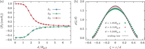
The effect of slit-like confinement on the average size, shape and orientation of the ring is illustrated in Figures 1–3. The overall behaviour closely resembles that of linear chains [66–70] and confirms the previously obtained results for rings [71,72]. In particular, for slit widths the size (see Figures 1 and 2(a,b)) and shape (see Figure 2(c)) of the ring remain nearly unaffected by the presence of the walls, although already in this regime its longest and middle principal axes start to orient parallely to the slit plane, whereas its smallest principal component tends to align orthogonally to it (see Figure 3(a)). This is caused by the fact that the monomer density distributions (indicated in Figure 3(b)) do not vanish in the proximity of the walls, which means that there exist a certain amount of oriented configurations of the ring contributing to the average of . Further narrowing of the slit () causes even stronger orientation of the eigenvectors and a simultaneous decrease in size of all the corresponding eigenvalues (see Figure 2(a,b)) with a minimum of the average size of the ring at about . In this regime, the polymer is squeezed along the z-direction more strongly than it is swollen along the two lateral directions, leading to an overall decrease in , manifesting itself as the characteristic dip around in the curve for the total gyration radius in Figure 1(a).

Figure 1. (a) Total () and in-plane () gyration radius of the ring polymer with N=250 monomers as a function of slit width d. Inset: a log–log plot of stressing its scaling behaviour accounted for de Gennes' blob theory. (b) Out-of-plane radius of gyration, , in dependence on d.

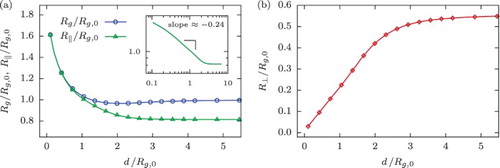
Figure 2. Eigenvalues of the gyration tensor, , for the ring polymer with N=250 monomers in dependence on slit width d and scaled (a) with the associated bulk values , , and (b) for the corresponding value of d. Ratios of the eigenvalues shown in panel (c) demonstrate a drastic asymmetry of the polymer for resulting in its overall ‘pancake’-shape.

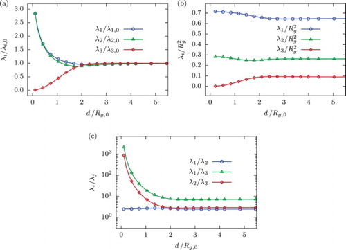
Figure 3. (a) Alignment of the eigenvectors of the radius of gyration tensor, , for a confined ring polymer with N=250 monomers quantified by means of the expectation value of the second Legendre polynomial  (8(8) ) as a function of slit width d. (b) Monomer density distributions for various values of slit widths as a function of , where z denotes the distance from the centre of the slit, in comparison to scaling formula (17(17) ) plotted with the solid grey line.

The excluded volume effects play the decisive role that causes drastic in-plane elongation of the ring as d shrinks only further on. In fact, the following behaviour can be observed for : the two biggest eigenvalues start rising abruptly, with the smallest one monotonically approaching zero such that the in-plane gyration radius, , gradually becomes that of a two-dimensional self-avoiding walk, according to de Gennes' blob representation [73], satisfying the following scaling relation: (16) with the scaling exponent , where the Flory exponents in good solvent are and for two and three dimensions, respectively. For this exponent, we obtain a value which lies below the one predicted by the de Gennes theory for linear chains and explicitly confirmed numerically for rings [71]. This can be explained by the fact that the considered ring with N=250 is not long enough to completely unfold the two-dimensional scaling behaviour. Finally, as expected for , the longest and middle principal components of the ring predominantly align parallel to the slit plane with the smallest one lying perpendicularly to it. Two larger eigenvalues are of the same order of magnitude but considerably exceed the smallest one (see Figure 2(c)), which results in an overall ‘pancake’-shape of the ring.

In addition, we compare the obtained monomer densities for the ring polymer to the following scaling formula valid for ideal and self-avoiding linear chains [67,74]: (17) where with z denoting the distance from the centre of the slit and . Density profiles for some characteristic values of slit width d are shown in Figure 3(b) and are in fair agreement with the ansatz (17(17) ). We also report that even better correspondence can be achieved using the variable , where δ is a non-universal fit parameter.

3.2. Single-wall confinement

Our next objective is to consider metric properties of the same ring polymer with a number of N=250 monomers as its centre of mass approaches a single, hard wall located at z=0. This is an important step to judge the validity of the effective ring–wall interaction, to be derived for a ring and a single wall in Section 4, also for the case of confinement between two walls, which is necessary for the calculation of the depletion interaction in Section 5. Indeed, to the extent that the presence of the second wall does not significantly affect the conformations of a ring whose centre of mass is held at a fixed separation from another, symmetrically positioned wall, additivity of the two ring–wall interactions can be safely assumed.

For these purposes, we introduced in our MC simulations an additional infinite well bias potential, which maintained the centre of mass of the polymer in a narrow ‘window’ of width centred at the distance h away from the wall for various values of h in the range . Similarly, for each value of h, statistics was gathered over – independent configurations, the resulting errors do not exceed and therefore are not shown in the plots.

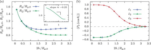
In general, the results obtained here closely resemble those for a ring polymer confined within a slit of width . In order to outline the differences between these two cases, Figure 4 includes the average size (4(a)) and orientation (4(b)) of the ring as a function of , i.e. at double the distance between its centre of mass and the wall, which can be directly compared to the results for a slit-like confinement shown in Figures 1(a) and 3(a), respectively. For instance, it can be easily seen in Figure 4(a) that in a similar way attains a minimum at about and then rises sharply for . At the same time, monotonically increases with decreasing h for . This behaviour, as in the case of slit-like confinement, is bound to the fact that the polymer enters the two-dimensional self-avoiding random walk (Equation (16(16) )) for which we find a similar value of the scaling exponent . However, the additional constraint of fixing the centre of mass position of the polymer at a certain distance away from the wall has a profound effect on its orientation: in contrast to the slit-confinement which shows some orientational preference for , the single-wall confined ring at practically does not experience the presence of the wall, featuring eigenvectors of its radius of gyration tensor distributed uniformly (compare Figure 3(a) to Figure 4(b)). However, these differences are small and they are not expected to lead to strong non-additivity effects for two walls in terms of the effective ring–wall potential.

Figure 4. (a) Total () and in-plane () gyration radius of the ring polymer with N=250 monomers as a function of the separation between its centre of mass and a hard wall, h. Inset: a log–log plot of emphasising its scaling behaviour. (b) Alignment of the eigenvectors of the ring's radius of gyration tensor, , quantified by means of the expectation value of the second Legendre polynomial , Equation (8(8) ), as a function of h. The values on the x-axis are doubled to be able to make a direct comparison to the results for the slit-like confinement.

We have therefore shown that the metric properties of a ring polymer with its centre of mass held at a distance h away from an impenetrable wall effectively resemble those for the polymer confined within a slit of width d=2h: in particular, for or , in both cases the ring gradually becomes two dimensional and deforms significantly with respect to the three-dimensional random walk regime (see Figure 5). This fact leads to a dramatic loss of entropy for rings constrained to lie either very close to a wall or within narrow slits of two walls, which manifests itself as a strongly repulsive, entropic, effective ring–wall interaction, to be discussed next.

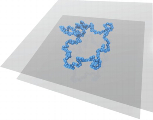
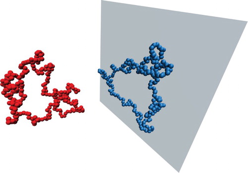
Figure 5. Representative conformations of a ring polymer far away (left) from and close (right) to a hard wall.

4. Coarse-graining of ring polymers on planar, hard walls

We carried out extensive umbrella sampling calculations for polymers of different degree of polymerisation N. Figure 6 shows the effective potentials as a function of the distance of the centre of mass away from the wall, for either ring (Figure 6(a)) or linear polymers (Figure 6(b)), for different degrees of polymerisation N. We observe that the effective potential in the ring polymer case collapses on a master curve in their natural units for 200, whereas the same holds for linear polymers already for 100. At least qualitatively, this difference can be understood as follows: on dimensional grounds, we can express the effective potential in terms of the fundamental energy and length scales of the system, as well as on N. If we make the assumption that the latter enters solely through the dependence of the gyration radius on N, then we expect an effective potential of the form (18) where φ is some dimensionless function, determines the energy scale of the system, whereas σ and designate the length scales on the monomer-resolved and coarse-grained level, respectively. Accordingly, on the coarse-grained level we can write (19) where we have used as an expansion parameter whose leading order in N scales as (), and are some other dimensionless functions. Most importantly, the numeric constant α that depends on the architecture of the polymers is larger for the rings in comparison to the linear chains, as their is smaller for a fixed N, and therefore the contribution arising from the term becomes negligible only for longer rings.

Figure 6. Effective potentials, , between the centre of mass of a polymer of ring (a) and linear (b) topology and a planar, hard wall given for various polymerisation degrees N. The dashed line in panel (b) corresponds to the ring with N= 250 monomers and is plotted to emphasise the difference between the effective interactions for the two polymer architectures considered.

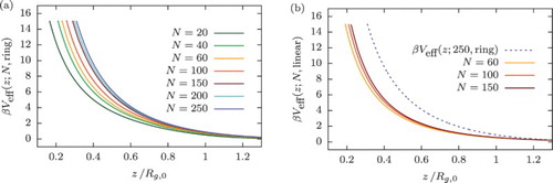
In Figure 6(b), we show the comparison between the effective wall potentials of the ring and linear polymers in the apparent scaling regime: we observe for rings a higher amplitude of the potential. This can be understood using a simple mean-field argument: a ring polymer coil having the same mean size as a linear polymer consists out of more monomers than the latter. Therefore, rings are expected to interact more often with the wall as the centre of mass of the coil approaches z=0 with respect to the linear counterpart. Obviously, this results in higher values of the interaction energy for a fixed z.

Following Bolhuis et al. [19] and Bolhuis and Louis [20], we fit the interaction potential of the coarse-grained polymer coils on hard walls with a cubic exponential function (z below is measured in units of ): (20) which provides a reasonable accuracy with numerical data. For the longest ring polymer considered (N=250), we obtain the following fit parameters: , , , . The corresponding values for the linear polymer case (N= 150) are , , , . Interestingly, close to the wall () the potentials for the both architectures studied can be very accurately described as a repulsive Yukawa interaction featuring comparable decay lengths but distinct amplitudes. However, the tail of a Yukawa-like functional form has a slower decay in comparison to numerical data, which results in a non-negligible difference in the fluid structure obtained from DFT calculations.

The obtained effective interaction of ring polymer on hard walls, in conjunction with the effective inter-ring potential [24–26], can be used to represent a ring polymer as a ‘soft-colloidal’ particle whose spatial degrees of freedom are described only by the former centre of mass position of the polymer. This enables us to study ring polymer solutions under confinement employing standard DFT methods outlined in Section 2. We first consider in detail the solution in contact with a single hard wall in Section 5 and then move on to the case of two hard walls presented in Section 6.

5. Ring polymer fluids near a hard wall

In this section, we apply DFT, briefly introduced in Section 2, to calculate the density profile of a solution of ring polymers in contact with a hard wall; as further characterisation, we calculate the surface tension at the interface between the fluid and the wall. We carry on the comparison with the linear case, showing that there are qualitative and quantitative differences between the two cases.

5.1. Structure of the equilibrium density profiles

Let us consider a ring polymer solution in contact with a planar, hard wall. Without loss of generality we assume that the system is enclosed by a large box with volume V and that the wall is located at z=0 confining the fluid to a half-space (note that the z-axis is orthogonal to the wall). The gyration radius of the polymers is adopted as the fundamental length scale of the system.

We can exploit the symmetries of the system in order to simplify Equation (15(15) ) further. First of all, we note that (21) Under such form of the external field, the equilibrium densities obtained from Equation (15(15) ) must depend on the z-coordinate only due to the preservation of the translation symmetry in the x- and y-directions: . Furthermore, the geometry of our setup ensures that for z<0. We obtain an explicit, one-dimensional self-consistency condition for the equilibrium profile , viz.: (22) where the following shorthand has been introduced: (23) Last, for we set (24) where goes to zero for large values of z (i.e. approaches as ). Substitution of Equation (24(24) ) into Equation (22(22) ) leads to the final form of the integral equation: (25) where we have used the identity stemming from the translational invariance of the integral. This equation can be solved numerically by iteration, until self-consistency between the short-ranged sought-for function on both sides has been achieved. Note that the bulk density, , is the only free parameter in integral equation (25(25) ) that has to be specified at the beginning of each numerical computation.

Equation (25(25) ) allows us to obtain the equilibrium structure of polymer solutions under a single-wall confinement, as long as the effective potentials and in the coarse-grained representation are specified. As already mentioned, in this article we are mainly interested in the ring polymer solutions. The effective interaction potential between the centres of mass of two rings [24] has been shown to be modelled very accurately by the following expression [25]: (26) where , , and , arising from overlap volumes between two unequal spheres of radii and , all lengths measured in units of . In conjunction with the effective external potential devised in the previous section, we have calculated density profiles of rings in contact with hard walls. We compare these profiles with the corresponding ones for linear chains, for which a Gaussian effective interaction between their centres of mass has been employed [20], subject to the external wall-chain potential given by Equation (20(20) ) and employing the parameters appropriate to linear chains. Here, the bulk polymer concentrations are expressed as ratios over the overlap density of the polymers, , the latter being defined by the relationship .

Figure 7 displays the resulting density profiles, expressed in terms of the quantity , obtained for increasing bulk density up to the onset of the semi-dilute regime (defined as ), for either ring (Figure 7(a)) or linear (Figure 7(b)) polymers. It is important to point out the crucial difference: in comparison to the linear chains, rings in solution feature a density profile with oscillations that intensify with higher values of . For the linear counterparts, we observe a non-oscillatory behaviour with a main peak close to the wall, whose height rises with the bulk density. In this sense, the density profiles of ring polymers close to hard walls are reminiscent of those obtained for much harder colloidal particles, such as hard spheres [75,76] or multiarm star polymers [77]. Both of the latter colloids are indeed strongly repulsive to one another, as well as to the wall, and thus the oscillatory profile is a natural consequence of the strong short-range correlations arising among them. It is quite astonishing that a similar phenomenology would arise also with ring polymers, which are merely single polymer chains with their two ends tied together. The reason behind these strong correlations is twofold: on the one hand, the ring–wall interactions are significantly more repulsive than their chain-wall counterparts. On the other, and more importantly, the nature of the ring–ring interaction, featuring a plateau at close ring–ring approaches, favours full ring overlaps as concentration grows and leads to the formation of composite clusters which strongly repel one another (the inter-cluster repulsion scales with the square of the population of the cluster). This peculiar form of self-organisation, which allows for the formation of cluster-like order even in the absence of repulsions [61,78], plays an important role in the emergence of the oscillatory density profiles of the rings, and it has been independently confirmed by monomer-resolved simulations of confined ring polymers [79].

Figure 7. Equilibrium density profiles as a function of obtained from DFT calculations at different densities, for (a) ring and (b) linear polymer solutions in contact with a hard, planar wall. Bulk densities are scaled with the overlap concentration defined as .

Finally, it is very important to emphasise the range of applicability of our DFT calculations. As reported in  [24], results obtained by ultrasoft colloid representation of flexible ring polymers significantly differ from full monomer-resolved simulations for densities higher than . In particular, the effective infinite-dilution pair potential of Equation (26(26) ) belongs to the -class of potentials with negative components in their Fourier spectra and, therefore, causes the formation of cluster crystals [61,78] as the fluid density goes into the semi-dilute regime. However, this feature is not reproducible in the monomer-resolved simulations of flexible ring polymers due to many-body interactions arising at higher densities. Nevertheless, as we can see in Figure 7(a), even in the dilute regime, the density profiles of the ring polymer solution in contact with the wall feature the oscillatory behaviour and thus show a qualitative difference in comparison to their linear counterparts. Finally, such structure of the ring polymer fluids under confinement gives a rise to the oscillating form of the depletion interaction between two plates immersed in it, which will be considered in Section 6.

5.2. Surface tension at the wall–liquid interface

Surface tension of the interface between a fluid and a planar, hard wall can be computed straightforwardly as the difference between the grand potential of the system per unit area in the presence and absence of the wall [56]: (27) where A is the area of the interface, denotes the grand potential of the fluid in contact with one hard wall and is the grand potential of the unconfined, bulk fluid. DFT offers an optimally suited framework to calculate the surface tension. To make our notation precise, we first consider the grand potential functional of Equation (9(9) ) for the case of a fluid in contact with a single wall, which we denote as , where L is the length of the system perpendicular to the wall. Minimising this quantity with respect to the density profile at a given chemical potential (or bulk density ), we obtain the grand potential of the fluid in contact with one hard wall and extending a (finite) length L perpendicularly to the wall, viz.: (28) The quantity of Equation (27(27) ) is simply the limit of as the system becomes semi-infinite. Accordingly, the surface tension γ is expressed as [76] (29) with the grand potential density and the pressure p of the bulk fluid expressed with the help of Equations (9(9) ) and (14(14) ) as (30)

It is straightforward to show within our DFT approach that the quantity contains one contribution that scales linearly with L and exactly cancels with the term pL in Equation (29(29) ), leaving thus γ as an intensive quantity. With being the equilibrium density profile and , we obtain, after some algebra, the surface tension γ in closed form as follows: (31) which makes it convenient to calculate γ, since the multiple integrals are convolutions, easily evaluated via Fourier transformations, which all exist because as . The obtained surface tension for the ring and linear polymer case is compared in Figure 8, where it can be seen that the former exceeds the latter approximately by a factor of two, even deep in the dilute regime. This effect arises from the much more strongly repulsive nature of the wall–ring interaction, as compared to the wall-chain potential but also from the stronger inter-ring repulsion , which gives the ring fluid a stronger, oscillatory structure next to the wall, and it enhances, therefore, also the entropic contribution to the surface tension, given by the first term in Equation (31(31) ).

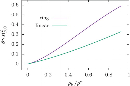
Figure 8. Surface tension at the interface between polymer solutions and the hard wall as a function of the bulk density, , obtained from DFT calculations.

6. Ring polymer fluids confined between two parallel walls

In this section, we apply DFT to calculate the depletion interaction caused by a solution of ring polymers confined between two hard walls. As previously mentioned, a slit-like confinement can be used as a model geometry to investigate the qualitative feature of depletion interactions. The depletion potential is, in this context, the penalty that arises from the decrease of the entropy of a fluid caused by the insertion of two surfaces, placed at a distance d. In order to address such problem, we first calculate the density profiles of the fluid in a slit-like confinement. We observe again the onset of an oscillatory behaviour in the density profile of the system that remains as a feature of the depletion interaction. Comparison with the linear case is presented for both quantities, showing drastic qualitative differences.

6.1. Structure of the equilibrium density profiles

We consider the following geometry of our setup: the first wall is placed at z=0, whereas the second one is located at the distance z=d>0 away from it. The total external field exerted on the fluid has then the following form: (32) As in the previous problem, symmetry arguments imply that . Moreover, in this case vanishes outside the interval and we expect its reflection-invariance with respect to the plane : .

Manipulations analogous to those performed in the previous section enable us to recast original integral equation (25(25) ) in the following form: (33) Obviously, the only difference between Equations (33(33) ) and (25(25) ) is the appearance of the term responsible for the interaction with the second wall located at z=d. In Figure 9, we show the resulting equilibrium density profiles for the ring (Figure 9(a)) and linear (Figure 9(b)) polymer solutions obtained for a fixed distance between the walls at various bulk densities. 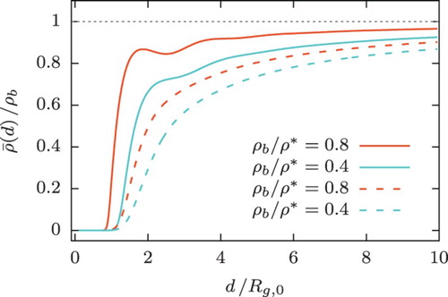As in the single-wall case, for high enough (or for small enough d) the rings, in comparison to the linear chains, exhibit strongly oscillatory density profiles, within the range of applicability of the effective model. These are reminiscent of the profiles obtained for hard-sphere solutions between two walls. In addition, Figure 10 displays the average density of polymers within a slit, , provided by (34) in dependence on its width, d, and the polymer architecture. It can be seen that rings, due to their higher mutual repulsion, tend to leak into the slit on average more than linear chains. Still, the average density within the slit remains lower than its value in the bulk.

Figure 9. Equilibrium density profiles as a function of obtained from DFT calculations at different densities, for (a) ring and (b) linear polymer solutions confined between two hard walls separated by the fixed distance .

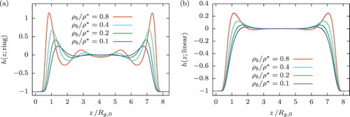
Figure 10. Average density of polymers, given by Equation (34(34) ), within a slit as a function of slit width obtained from DFT calculations at various bulk densities. Results for ring polymers are represented by solid lines, whereas those for linear chains by dashed ones.

6.2. The depletion potential

Finally, we turn our attention to the depletion potential between two infinite, hard walls, separated by a distance d and immersed in a solution of (ring or linear) polymers of bulk density . Formally, the depletion potential is defined as the difference of the grand potential of the whole system between its value at wall separation d and its value at some other reference separation between the walls, usually taken as the limit , at fixed overall system volume [75,80,81]. Once more, DFT offers us a suitable framework to calculate this quantity. To this purpose, we first consider the laterally averaged variational grand canonical density functional for the part of the fluid confined between two walls at separation d (i.e. excluding the fluid outside the walls). From the general form of the functional, Equation (9(9) ), it follows that (35) where A is the walls' area. In analogy with Equation (28(28) ), we define the grand potential of the confined fluid, , as (36) Let be precisely the density profile that minimises the functional and set . It is straightforward to show the following: (37) Comparing Equation (37(37) ) with Equation (31(31) ), we readily obtain that in the limit of large inter-wall separation, , the quantity reduces to a bulk contribution from the fluid within the walls, , augmented by twice the surface tension γ, due to the presence of two liquid–wall interfaces, as it should. Note that in this limit the superposition holds true, where is the density profile minimising the grand potential functional in the presence of a single wall.

On the other hand, the whole system occupies a total volume in a box of cross-sectional area A and length L. Accordingly, the fluid outside the confined walls forms two wall–fluid interfaces that bring forward a grand potential cost , in addition to a bulk grand potential contribution equal to . Accordingly, the rest of the system has a grand potential contribution (38) Letting (39) denote the grand potential of the entire fluid and the immersed walls, the depletion potential is defined as (40) It can be readily seen from Equations (37(37) ) and (38(38) ) that the terms involving cancel, leaving at only a term , which then also disappears from by virtue of Equation (40(40) ). The final expression for thus reads as (41)

Within our mean-field density functional, we can thus obtain the depletion potential (per unit area) for two parallel, infinite walls in closed form from Equation (41(41) ). A direct comparison with Equation (31(31) ) readily confirms that all the d-dependent terms at the right-hand side of Equation (41(41) ) add up to as , consistent with the property . At zero wall separation, on the other hand, the infinitely extending fluid forms two interfaces with the walls (since the fluid itself is completely depleted from the wall interior and only the two exterior interfaces remain), whereas at infinite wall separation four such interfaces are formed, two for each wall. Accordingly, a gain of in the grand potential of the system results when the two walls coincide, which is precisely the depth of of Equation (41(41) ) at d=0, where all integrals on the right-hand side vanish. Finally, assuming that for , the inter-wall space remains essentially uninvaded from the polymers due to the strong wall–polymer repulsion, the depletion force per unit area on each wall should equal the unbalanced osmotic pressure of the polymer solution. An expansion of the right-hand side of Equation (41(41) ) for small d, assuming there, yields: (42) the term in the parentheses at the right-hand side being indeed the bulk pressure, see Equation (30(30) ).

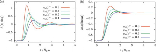
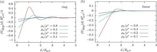
Figure 11 depicts the depletion potential between two hard walls immersed in ring (Figure 11(a)) or linear (Figure 11(b)) polymer solutions as a function of the slit size d, for various bulk densities. As anticipated from the equilibrium density profiles, in the dilute regime the depletion potential in the ring polymer case preserves an oscillatory shape with a maximum at about at the highest density considered exhibiting a drastic difference compared to the case of linear chains. Moreover, a similar oscillatory feature of the depletion potential is seen as the one arising can be found in hard-sphere mixtures [75,76,80–82] or hard-sphere–star polymer mixtures [33,34], although the depletants are simple unbranched polymers, only having the two ends attached. We anticipate that colloid–ring-polymer mixtures will behave very differently from colloid–linear-polymer mixtures, for which the depletion interaction is void of oscillatory features, and it thus causes a liquid–gas coexistence when the attraction is sufficiently strong [16]. Finally, we note that Equation (42(42) ) is fulfilled with remarkable accuracy up to inter-wall separations , where the depletion potential is indeed a linear function of the wall separation d.

Figure 11. Depletion potential per unit area between two hard walls immersed in a dilute (a) ring and (b) linear polymer solution as a function of obtained from DFT calculations at different densities in the bulk.

7. Conclusions

We have studied, by means of MC simulations and mean-field DFT calculations, the behaviour of dilute solutions of flexible ring polymers under confinement, systematically comparing our results with the linear counterparts. We have first analysed the conformational properties of a flexible ring polymer, when confined within a slit of width d or kept fixed at a distance d/2 away from a single hard wall. With such choice of the length scales in both cases we observe similar effects of confinement of the average size and orientation of the polymer. In particular, the coil starts to align its two bigger principal axes along the in-plane direction already for , whereas its average size rises abruptly only for . The latter point indicates a transition of the polymer to the two-dimensional random walk dynamics. We have further computed the effective interaction between the centre of mass of a ring polymer and a planar and impenetrable wall, for various degree of polymerisation. The resulting effective potentials approach a universal, functional form for and feature much higher interaction energies in comparison to the case of linear chains. We have then complemented this result with the well-established potential of mean force between two ring polymers to develop a coarse-grained model of the ring fluid under confinement. Note that the form of the effective ring–ring interaction, which was initially obtained for two unconfined polymers, will certainly change in the vicinity of the wall, where the rings essentially resemble disk-like objects. However, we expect that this effect has a marginal influence on the structure of the fluid for away from the wall. The effective fluid has been studied in contact with one and two hard walls employing standard DFT methods: we have shown that, in both cases, the resulting density profiles in the dilute concentration regime feature an oscillating profile reminiscent of hard-sphere systems. This effect mainly originates from the unique form of effective ring–ring interaction, which is caused by topological constraints, and cannot be observed in solutions of linear chains. Finally, we have calculated the depletion potential between two plates immersed in the ring polymer solution, which also preserves the aforementioned oscillatory shape and therefore shows a drastic difference to the linear counterparts. Future work will focus on the extension of the above-described approach to the mixtures composed of spherical, hard colloids and flexible ring polymers and to the consequences of this on the structure and phase behaviour of the system.

Acknowledgements

It is a pleasure and an honour to dedicate this paper to Prof. Daan Frenkel on the occasion of his 70th birthday. Daan's pioneering work on a broad variety of scientific fields – soft matter and condensed matter physics, physical chemistry, computer simulations and self-assembly, to mention a few of them – as well as the many personal exchanges with him have always been a constant sources of inspiration for all of us. Happy birthday, Daan!

Disclosure statement

No potential conflict of interest was reported by the authors.

References

- M.D. Frank-Kamenetskii, A.V. Lukashin and A.V. Vologodskii, Nature 258, 398 (1975). doi: 10.1038/258398a0
- C. Micheletti, D. Marenduzzo and E. Orlandini, Phys. Rep. 504 (1), 1 (2011). doi: 10.1016/j.physrep.2011.03.003
- S.S. Jang, T. Çağin and W.A. Goddard, J. Chem. Phys. 119 (3), 1843 (2003). doi: 10.1063/1.1580802
- A. Narros, A.J. Moreno and C.N. Likos, Macromolecules 46 (9), 3654 (2013). doi: 10.1021/ma400308x
- M. Kapnistos, M. Lang, D. Vlassopoulos, W. Pyckhout-Hintzen, D. Richter, D. Cho, T. Chang and M. Rubinstein, Nat. Mater. 7, 997 (2008). doi: 10.1038/nmat2292
- D. Marenduzzo, E. Orlandini, A. Stasiak, L. Tubiana and C. Micheletti, Proc. Natl. Acad. Sci. USA 106 (52), 22269 (2009). doi: 10.1073/pnas.0907524106
- D. Marenduzzo, C. Micheletti and E. Orlandini, J. Phys. Condens. Matter 22 (28), 283102 (2010). doi: 10.1088/0953-8984/22/28/283102
- A. Leforestier, A. Šiber, F. Livolant and R. Podgornik, Biophys. J. 100 (9), 2209 (2011). doi: 10.1016/j.bpj.2011.03.012
- D. Reith, P. Cifra, A. Stasiak and P. Virnau, Nucleic Acids Res. 40 (11), 5129 (2012). doi: 10.1093/nar/gks157
- T.A. Shapiro and P.T. Englund, Annu. Rev. Microbiol. 49 (1), 117 (1995). doi: 10.1146/annurev.mi.49.100195.001001
- J. Chen, C.A. Rauch, J.H. White, P.T. Englund and N.R. Cozzarelli, Cell 80 (1), 61 (1995). doi: 10.1016/0092-8674(95)90451-4
- D. Michieletto, D. Marenduzzo and E. Orlandini, Phys. Biol. 12 (3), 036001 (2015). doi: 10.1088/1478-3975/12/3/036001
- A. Grosberg, Y. Rabin, S. Havlin and A. Neer, Europhys. Lett. 23 (5), 373 (1993). doi: 10.1209/0295-5075/23/5/012
- A. Rosa and R. Everaers, PLOS Comput. Biol. 4 (8), e1000153 (2008). doi: 10.1371/journal.pcbi.1000153
- A. Rosa, Biochem. Soc. Trans. 41, 612 (2013). doi: 10.1042/BST20120330
- C.N. Likos, Phys. Rep. 348, 267 (2001). doi: 10.1016/S0370-1573(00)00141-1
- C.N. Likos, Soft Matter 2, 478 (2006). doi: 10.1039/b601916c
- A.A. Louis, P.G. Bolhuis, J.P. Hansen and E.J. Meijer, Phys. Rev. Lett. 85, 2522 (2000). doi: 10.1103/PhysRevLett.85.2522
- P.G. Bolhuis, A.A. Louis, J.P. Hansen and E.J. Meijer, J. Chem. Phys. 114 (9), 4296 (2001). doi: 10.1063/1.1344606
- P.G. Bolhuis and A.A. Louis, Macromolecules 35 (5), 1860 (2002). doi: 10.1021/ma010888r
- V. Krakoviack, J.P. Hansen and A.A. Louis, Phys. Rev. E 67, 041801 (2003). doi: 10.1103/PhysRevE.67.041801
- C. Pierleoni, B. Capone and J.P. Hansen, J. Chem. Phys. 127 (17), 171102 (2007). doi: 10.1063/1.2803421
- M. Bohn and D.W. Heermann, J. Chem. Phys. 132 (4), 044904 (2010). doi: 10.1063/1.3302812
- A. Narros, A.J. Moreno and C.N. Likos, Soft Matter 6, 2435 (2010). doi: 10.1039/c001523g
- A. Narros, A.J. Moreno and C.N. Likos, Macromolecules 46 (23), 9437 (2013). doi: 10.1021/ma4016483
- A. Narros, A.J. Moreno and C.N. Likos, Biochem. Soc. Trans. 31, 630 (2013). doi: 10.1042/BST20120286
- A. Narros, C.N. Likos, A.J. Moreno and B. Capone, Soft Matter 10, 9601 (2014). doi: 10.1039/C4SM01904K
- M. Bernabei, P. Bacova, A.J. Moreno, A. Narros and C.N. Likos, Soft Matter 9, 1287 (2013). doi: 10.1039/C2SM27199K
- P. Poier, C.N. Likos, A.J. Moreno and R. Blaak, Macromolecules 48 (14), 4983 (2015). doi: 10.1021/acs.macromol.5b00603
- P. Poier, S.A. Egorov, C.N. Likos and R. Blaak, Soft Matter 12, 7983 (2016). doi: 10.1039/C6SM01453D
- P. Poier, P. Bacova, A.J. Moreno, C.N. Likos and R. Blaak, Soft Matter 12, 4805 (2016). doi: 10.1039/C6SM00430J
- C.N. Likos, H. Löwen, M. Watzlawek, B. Abbas, O. Jucknischke, J. Allgaier and D. Richter, Phys. Rev. Lett. 80, 4450 (1998). doi: 10.1103/PhysRevLett.80.4450
- J. Dzubiella, C.N. Likos and H. Löwen, Europhys. Lett. 58 (1), 133 (2002). doi: 10.1209/epl/i2002-00615-y
- J. Dzubiella, C.N. Likos and H. Löwen, J. Chem. Phys. 116 (21), 9518 (2002). doi: 10.1063/1.1474578
- C. Pierleoni, C. Addison, J.P. Hansen and V. Krakoviack, Phys. Rev. Lett. 96, 128302 (2006). doi: 10.1103/PhysRevLett.96.128302
- B. Capone, C. Pierleoni, J.P. Hansen and V. Krakoviack, J. Phys. Chem. B 113 (12), 3629 (2009). doi: 10.1021/jp805946z
- C.N. Likos, S. Rosenfeldt, N. Dingenouts, M. Ballauff, P. Lindner, N. Werner and F. Vögtle, J. Chem. Phys. 117 (4), 1869 (2002). doi: 10.1063/1.1486209
- B. Lonetti, M. Camargo, J. Stellbrink, C.N. Likos, E. Zaccarelli, L. Willner, P. Lindner and D. Richter, Phys. Rev. Lett. 106, 228301 (2011). doi: 10.1103/PhysRevLett.106.228301
- C. Mayer and C.N. Likos, Macromolecules 40, 1196 (2007). doi: 10.1021/ma062117z
- D. Truzzolillo, D. Marzi, J. Marakis, B. Capone, M. Camargo, A. Munam, F. Moingeon, M. Gauthier, C.N. Likos and D. Vlassopoulos, Phys. Rev. Lett. 111, 208301 (2013). doi: 10.1103/PhysRevLett.111.208301
- D. Marzi, B. Capone, J. Marakis, M.C. Merola, D. Truzzolillo, L. Cipelletti, F. Moingeon, M. Gauthier, D. Vlassopoulos, C.N. Likos and M. Camargo, Soft Matter 11, 8296 (2015). doi: 10.1039/C5SM01551K
- E. Locatelli, B. Capone and C.N. Likos, J. Chem. Phys. 145 (17), 174901 (2016). doi: 10.1063/1.4965957
- A.Y. Grosberg, P.G. Khalatur and A.R. Khokhlov, Macromol. Chem. Rapid Commun. 3 (10), 709 (1982). doi: 10.1002/marc.1982.030031011
- B. Kruger, L. Schäfer and A. Baumgärtner, J. Phys. France 50 (21), 3191 (1989). doi: 10.1051/jphys:0198900500210319100
- H. Lekkerkerker and R. Tuinier, Colloids and the Depletion Interaction, Vol. 833 (Springer, Berlin, 2011).
- S. Asakura and F. Oosawa, J. Chem. Phys. 22 (7), 1255 (1954). doi: 10.1063/1.1740347
- S. Asakura and F. Oosawa, J. Polym. Sci. 33 (126), 183 (1958). doi: 10.1002/pol.1958.1203312618
- A. Vrij, Pure Appl. Chem. 48 (4), 471 (1976). doi: 10.1351/pac197648040471
- Y. Mao, M.E. Cates and H.N.W. Lekkerkerker, Phys. Rev. Lett. 75 (24), 4548 (1995). doi: 10.1103/PhysRevLett.75.4548
- Y. Mao, M.E. Cates and H.N.W. Lekkerkerker, J. Chem. Phys. 106, 3721 (1997). doi: 10.1063/1.473424
- L. Harnau and S. Dietrich, Phys. Rev. E 69, 051501 (2004). doi: 10.1103/PhysRevE.69.051501
- G.S. Grest and K. Kremer, Phys. Rev. A 33, 3628 (1986). doi: 10.1103/PhysRevA.33.3628
- D. Frenkel and B. Smit, Understanding Molecular Simulation, 2nd ed. (Academic Press, Inc., Orlando, FL, 2001).
- R. Blaak, B. Capone, C.N. Likos and L. Rovigatti, Computational Trends in Solvation and Transport in Liquids, edited by G. Sutmann, J. Grotendorst, G. Gompper and D. Marx. Lecture Notes, IAS Series (Forschungszentrum Jülich, Jülich, 2015), Vol. 28, pp. 209–250.
- D.N. Theodorou and U.W. Suter, Macromolecules 18 (6), 1206 (1985). doi: 10.1021/ma00148a028
- J.P. Hansen and I.R. McDonald, Theory of Simple Liquids, 4th ed. (Elsevier, Amsterdam, 2013).
- P. Hohenberg and W. Kohn, Phys. Rev. 136, B864 (1964). doi: 10.1103/PhysRev.136.B864
- N.D. Mermin, Phys. Rev. 137, A1441 (1965). doi: 10.1103/PhysRev.137.A1441
- R. Evans, Adv. Phys. 28 (2), 143 (1979). doi: 10.1080/00018737900101365
- A. Lang, C.N. Likos, M. Watzlawek and H. Löwen, J. Phys. Condens. Matter 12 (24), 5087 (2000). doi: 10.1088/0953-8984/12/24/302
- C.N. Likos, A. Lang, M. Watzlawek and H. Löwen, Phys. Rev. E 63 (3), 031206 (2001). doi: 10.1103/PhysRevE.63.031206
- A.A. Louis, P.G. Bolhuis and J.P. Hansen, Phys. Rev. E 62, 7961 (2000). doi: 10.1103/PhysRevE.62.7961
- A.J. Archer and R. Evans, Phys. Rev. E 64, 041501 (2001). doi: 10.1103/PhysRevE.64.041501
- A.J. Archer and R. Evans, J. Phys. Condens. Matter 14 (6), 1131 (2002). doi: 10.1088/0953-8984/14/6/302
- A.J. Archer, C.N. Likos and R. Evans, J. Phys. Condens. Matter 14 (46), 12031 (2002). doi: 10.1088/0953-8984/14/46/311
- J.H. Van Vliet, M.C. Luyten and G. Ten Brinke, Macromolecules 25 (14), 3802 (1992). doi: 10.1021/ma00040a029
- D.J. Bonthuis, C. Meyer, D. Stein and C. Dekker, Phys. Rev. Lett. 101, 108303 (2008). doi: 10.1103/PhysRevLett.101.108303
- J. Tang, S.L. Levy, D.W. Trahan, J.J. Jones, H.G. Craighead and P.S. Doyle, Macromolecules 43 (17), 7368 (2010). doi: 10.1021/ma101157x
- J. Chen and D.E. Sullivan, Macromolecules 39 (22), 7769 (2006). doi: 10.1021/ma060871e
- D.I. Dimitrov, A. Milchev, K. Binder, L.I. Klushin and A.M. Skvortsov, J. Chem. Phys. 128 (23), 234902 (2008). doi: 10.1063/1.2936124
- C. Micheletti and E. Orlandini, Macromolecules 45 (4), 2113 (2012). doi: 10.1021/ma202503k
- R. Matthews, A.A. Louis and J.M. Yeomans, Mol. Phys. 109, 1289 (2011). doi: 10.1080/00268976.2011.556094
- P.G. De Gennes, Scaling Concepts in Polymer Physics (Cornell University Press, Ithaca, NY, 1979).
- H.P. Hsu and P. Grassberger, J. Chem. Phys. 120 (4), 2034 (2004). doi: 10.1063/1.1636454
- B. Götzelmann, R. Evans and S. Dietrich, Phys. Rev. E 57, 6785 (1997). doi: 10.1103/PhysRevE.57.6785
- R. Roth and S. Dietrich, Phys. Rev. E 62, 6926 (2000). doi: 10.1103/PhysRevE.62.6926
- J. Dzubiella, H.M. Harreis, C.N. Likos and H. Löwen, Phys. Rev. E 64, 011405 (2001).
- C.N. Likos, B. Mladek, D. Gottwald and G. Kahl, J. Chem. Phys. 126 (22), 224502 (2007). doi: 10.1063/1.2738064
- L.B. Weiß, A. Nikoubashman and C.N. Likos, Semidilute polymer solutions in microfluidic devices, 2018 (unpublished).
- B. Götzelmann, R. Roth, S. Dietrich, M. Dijkstra and R. Evans, Europhys. Lett. 47 (3), 398 (1999). doi: 10.1209/epl/i1999-00402-x
- R. Roth, R. Evans and S. Dietrich, Phys. Rev. E 62, 5360 (2000). doi: 10.1103/PhysRevE.62.5360
- A.A. Louis, E. Allahyarov, H. Löwen and R. Roth, Phys. Rev. E 65, 061407 (2002). doi: 10.1103/PhysRevE.65.061407