Controlling observables in normal, hybrid and Josephson junctions

ABSTRACT

The theory of time-dependent quantum transport addresses the question: How do electrons flow through a junction under the influence of an external perturbation as time goes by? In this article, we invert this question and search for a time-dependent bias such that the system behaves in a desired way. Our system of choice consists of quantum dots coupled to normal or superconducting leads. We present results for junctions with normal leads where the current, the density or a molecular vibration is optimised to follow a given target pattern. For junctions with two superconducting leads, where the Josephson effect triggers the current to oscillate, we investigate what happens if the frequency of the Josephson oscillation comes close to the frequency of the molecular vibration. Furthermore we show how to suppress the Josephson oscillations by suitably tailoring the bias. In a second example involving superconductivity, we consider a Y-shaped junction with two quantum dots coupled to one superconducting and two normal leads. This device is used as a Cooper pair splitter to create entangled electrons on the two quantum dots. We maximise the splitting efficiency with the help of an optimised bias.

GRAPHICAL ABSTRACT

KEYWORDS:

• Molecular electronic devices
• superconductivity
• vibrations
• non-equilibrium processes in superconductivity
• Cooper pairs

1. Introduction

Molecular quantum transport is a fast growing research field. The ultimate goal is to produce electronic devices using single molecules as their building blocks [1–4]. The prospective improvements regarding operational speed as well as storage capacity are expected to be enormous if the miniaturisation of transistors can be taken to the scale of single molecules.

In the past, the main objective was to measure and/or calculate the current-voltage characteristics of the molecular junction. On the theory side, calculations were usually done within the Landauer-Büttiker approach. In recent years, interest has shifted more and more towards time-resolved studies. Such studies allow one to address questions like: How long does it take until the steady state is reached? Can we shorten or lengthen this time span? Does a steady state always exist, and if so, is it unique? To answer this kind of questions by calculations, explicitly time-dependent approaches are necessary, such as time-dependent density functional theory [5–12], the Kadanoff–Baym equations [13–16], multi-configuration time-dependent Hartree–Fock [17–20], Quantum Monte-Carlo [21], time-dependent tight binding [22–24], or the hierarchy equation of motion approach [25–27].

In all those approaches the reaction of the molecular junction to a given external perturbation, i.e. a bias or a gate voltage is calculated. In this article, we want to take a step beyond this point and control the current or other observables of the junction. This means we have to address the inverse question: Which perturbation leads to a desired reaction of the system? To answer this question, optimal control theory provides a suitable framework. This research field was pioneered by the work of Pontryagin et al. [28] and Bellman [29] who paved the way for numerous applications. Initially, optimal control theory was mainly used to solve problems of classical mechanics. Later, it found applications in many other research fields including quantum mechanics [30–35].

A particularly interesting field goes under the heading of ‘femto-chemistry’ where chemical reactions are influenced with femto-second laser pulses such that a specific reaction gets suppressed or enhanced [36–39]. A successful experimental application is the selective bond dissociation of molecules [40]. Other applications of optimal control theory in the quantum world include the control of the electron flow in a quantum ring [34], the accelerated cooling of molecular vibrations [41], the control of the entanglement of electrons in quantum wells [42], the optimisation of quantum revival [43], the control of ionisation [44,45] or the selection of transitions between molecular states [46].

Kleinekathöfer and coworkers combined optimal control theory with the master equation approach for quantum transport and demonstrated the control of various observables in junctions with normal leads [47–49]. We take a different approach to the same problem by propagating wave functions. For the time propagation, we employ an algorithm proposed by Stefanucci et al. [50]. This allows us to treat not only normal (N) but also superconducting (S) leads.

The paper is organised as follows: In Section 2, we explain the model Hamiltonian that we employ to describe the molecular junctions. In Section 3, we formulate the optimisation problem for tailoring the bias such that a chosen observable follows a predefined pattern as best as possible. Various results are presented in Section 4. Finally, in Section 5, we focus on a specific example, a Y-shaped junction consisting of two quantum dots coupled to one superconducting and two normal leads. This device is used as a Cooper-pair splitter, for which we maximise the splitting efficiency. In the final Section 6, we draw our conclusions.

2. Model

2.1. Static quantum dot

Our model system consists of a quantum dot (QD) connected to two semi-infinite, non-interacting one dimensional leads (L and R), which are described by a tight binding Hamiltonian. Later, in Section 5, we will add a third lead (labelled S) and a second quantum dot. The corresponding changes in the Hamiltonian will then be stated in that section but the overall approach and the structure of the equations stays the same.

The Hamiltonian for the junction with two leads and a single quantum dot reads (1) with (2) (3) (4)

Here are the Peierls' phases with the bias . The operator () creates (annihilates) an electron at site in the lead with spin . The operator () represents the creation (annihilation) of an electron on the quantum dot.

The observables of prime interest, the density and the current , are given by (5) (6)

All parameters in Equations (1(1) )–(4(4) ) are real and positive. We always work at temperature T=0 and in the wide band limit , where the coupling to the leads is given by . In this limit, the results only depend on the couplings but not on the hopping elements individually. The superconducting pairing potentials can be written as , which allows a dimensionless representation of the problem by measuring times in units of and energies as well as currents in units of . In the case of normal leads, we set , and otherwise. The presence of superconductivity requires the propagation of the time-dependent Bogoliubov–de Gennes equation (7) (8)

The non-vanishing elements of and can be grouped as follows:

1. Central region (9)

2. Leads (10) (11) for lead α

3. Coupling of quantum dot to lead α (12)

The single-particle wave functions (13) represent the time-dependent particle- and hole-ampli-tudes at site k. The algorithm for the time propagation of the single particle wave functions as well as the initial state calculation is explained in the work of Stefanucci et al. [50], which extends the method of Kurth et al. [8] to superconducting leads.

2.2. Classical vibrations

In this paragraph, we extend the model to incorporate a vibrational degree of freedom in the central region. In the past, most theoretical work focussed on the electronic system and neglected the nuclear motion. In experiments, the nuclei are, of course, not fixed to a position and their motion can have a significant influence on the measured properties, for example on the current-voltage characteristics [51–54].

The vibrational degree of freedom is described within the Ehrenfest approximation following Verdozzi et al. [55]. The modified central part of the electronic Hamiltonian reads (14)

The parameter λ determines the interaction strength between the electronic and the nuclear system. The equation of motion for the vibrational coordinate is (15) (16)

The above model can be viewed as a classical version of a polaron model [56]. The validity of this model has been discussed [57] for the normal conducting case, revealing that the description is not a mean field approximation but exact in the static limit . This limit corresponds to a vibrational motion that is slow compared to the electronic timescale. The same holds for our model in the static limit with large masses and slow changes of the bias [57].

Recently, a comparative study of Ehrenfest dynamics and exact results for the polaron model in a finite system showed quantitatively similar behaviour, but the time scales can be different [58]. This suggests quantitatively good results even away from the static limit.

In all calculations, the coupling parameter λ is chosen positive and the mass m will be set to . Γ and are chosen such that the condition is well-satisfied.

Equations (7(7) ) and (16(16) ) are propagated in time starting from an initial position and initial single particle wave functions . The latter are chosen to represent the ground state of the system, which is calculated using a self-consistency cycle of electronic and vibrational part [50,55].

2.3. Resonance of the Josephson frequency and the vibration

In junctions with two superconducting leads, the Josephson effect causes the current to oscillate. This offers a unique way to drive the molecular vibration by tuning the DC bias such that the Josephson frequency is in resonance with the vibrational degree of freedom. This is shown in Figures 1 and 2.

Figure 1. Top: Absolute value of the time average of the position . Bottom: Amplitude of the oscillations of . The vertical line represents the pure vibrational frequency transformed into a bias via the Josephson frequency relation . The parameters are: , and .

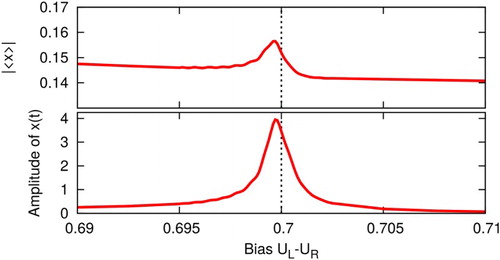
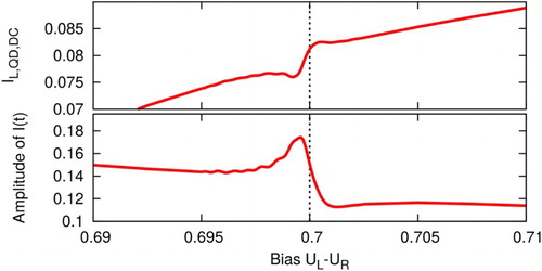
Figure 2. The same simulation as Figure 1 but showing results for the current. Top: Time averaged current-voltage characteristics for an SQDS junction. Bottom: Amplitude of the oscillations of as a function of the applied bias.

We make the following observations:

1. As a function of the applied bias (and hence as a function of the Josephson frequency ), the amplitude of the Josephson-effect-driven vibration has the shape of a driven harmonic oscillator (see Figure 1 lower panel).

2. The peak of the amplitude is shifted compared to the frequency of the pure vibration similar to a damped driven harmonic oscillator.

3. The absolute value of the time average of the classical coordinate, i.e. the average distance between the vibrating nuclei, becomes slightly larger at the resonance and has two different values above and below the resonance. Note that this effect is by 2−3 orders of magnitude smaller than the enhancement of the amplitude.

4. The current as a function of the bias shows a resonance effect as well: The DC part shows a down-up variation near the resonance within the otherwise linear behaviour.

5. The amplitude of the oscillatory part has a relatively sharp maximum at the resonance and has different values above and below the resonance. The peak is again slightly shifted towards smaller biases.

Since the amplitude of the current can easily be measured in experiments, the above effects provide a way of accurately determining the vibrational frequency of the molecule in the junction. The signatures in the current-voltage characteristics are much sharper than those produced by photon assisted tunnelling, a fact which can be exploited experimentally to determine vibrational frequencies [59].

3. Optimisation problem

We start at t=0 in the ground state of the junction with . The goal is to tailor the bias such that the observable of choice follows a predefined target pattern as best as possible. The corresponding optimisation problem reads (17) where

Here, denotes the -norm on the time interval , i.e. the objective function is the following integral: (18)

The integral is well-defined since T and the integrand are finite in all examples studied in this work.

Most common is a variational approach to this problem, like the Rabitz approach [60] or Krotov's method [61,62]. Such an approach incorporates the constraints into the objective function using Lagrange multipliers and searches for the roots of the variation of the new objective function. An alternative approach, which we shall adopt in this article, is the direct minimisation of the objective function using derivative-free minimisation algorithms. This strategy was successfully used in several works [44,63–65]. In this way, we avoid various difficulties arising from the time propagation algorithm. This approach can be viewed as the computational analogue to the closed-loop learning algorithms employed in experimental optimisation [66].

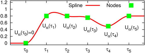
The basic idea of our numerical approach is to approximate by cubic splines with N+1 equidistant nodes at . We choose as the boundary conditions for the splines. The dependence of the problem (17(17) ) on the bias is replaced by (19) In this way, the spline-interpolated bias becomes a function of . This then yields a normal nonlinear optimisation problem with the unknown variables . We further impose the condition since the bias has to be continuous and we assume . Figure 3 demonstrates this approach.

Figure 3. Cubic spline interpolation using six nodes . The optimisation algorithm changes the values . The value is fixed to zero. The derivatives at both ends are set to zero. The spline does not necessarily take the maximum or minimum value at one of the nodes. In this example, the maximum lies between and .

Additionally, we add the constraint unless otherwise stated, since it reduces the dimensionality of the optimisation problem in the numerical implementation by a factor of two. This implies the constraint . The resulting nonlinear optimisation problem is (20) where

The single particle wave functions in problem (20(20) ) are only auxiliary variables. Hence, the time-dependent Bogoliubov–de Gennes equation can be removed from the constraint equations for the numerical implementation. The objective function is then written as , whose evaluation requires us to solve the time-dependent Bogoliubov–de Gennes equation in order to calculate the observable .

Problem (20(20) ) can be solved using standard derivative-free algorithms for nonlinear optimisation problems. We use the algorithms BOBYQA [67] or COBYLA [68,69] provided by the library NLopt [70]. The former one does not support nonlinear constraints, but converges faster compared to other tested methods. The latter algorithm will be used for the calculations with nonlinear constraints.

We point out that the quality of the results depends on the number of nodes for the splines. A larger number N is typically favourable for better results, i.e. yields a better match of the observable with its target pattern . But, the computational cost increases with N. In simple test cases of a NQND junction, we observe that the cost, i.e. the number of evaluation of the objective function, scales approximatelly as for the algorithm BOBYQA. For the minimal value of the objective funtion, we observe as scaling behaviour approximately of . Thus, the overall convergence rates of the proposed procedure are good. Besides, it is not guaranteed that the obtained minimum is the global minimum since the used algorithms are local optimisation algorithms. Thus, the results may depend on the initial choice for .

We now discuss how to control the nuclear motion using the bias as before. Although the bias couples only to the electronic part of the system, it induces changes in the density which in turn influences the nuclear motion. Hence, the electrons mediate between the bias and the vibration. The feasibility of controlling the nuclear motion in a quantum-classical system has already been demonstrated [71].

The optimisation problem for controlling the vibrational coordinate then reads (21) where

4. Results of optimisation

4.1. Current and density of a NQDN junction

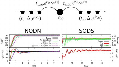
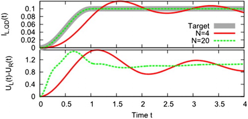
As a first example, we show the optimisation of the current from the left lead onto the quantum dot. This is done for two different numbers of spline nodes N. As shown in Figure 4 the case N=4 shows strong deviations while N=20 already yields an excellent agreement of the calculated current with its target pattern.

Figure 4. NQDN junction with an optimised current for two different numbers of spline nodes N. The parameters are: .

The optimisation of the density is very similar to the optimisation of a current, one simply exchanges the observable in the objective function. An example is shown in Figure 5. The density follows perfectly the target pattern.

Figure 5. NQDN junction with an optimised density. The parameters are: .

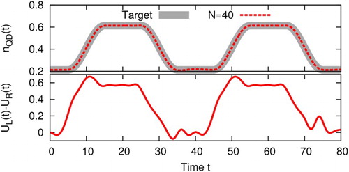
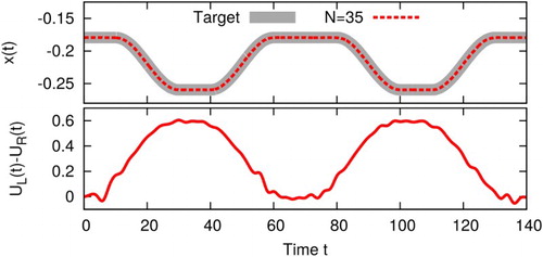
Figure 6 shows an example of controlling the nuclear motion, forcing the classical coordinate to follow a given target function .

Figure 6. NQDN junction with an optimised position of a vibration coupled to the quantum dot. The parameters are: .

4.2. Imposing further constraints on the bias

In real-world control experiments, an arbitrary time-dependence of is difficult to achieve. In this section, we therefore impose further constraints to restrict the bias or the derivative . The optimisation problem including such additional constraints then reads (22) where

The conditions are in general not equivalent to , unless one uses a monotonic cubic spline. This can be seen in Figure 3, where the maximum value of the spline lies between and . The constraint for the time derivative is not accessible in this way.

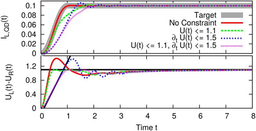
The cubic spline is a third degree polynomial between two nodes and . Thus, the minimum and maximum values can be calculated analytically in every interval . The constraints are replaced by (23) (24) (25) (26) for . Figure 7 shows the influence of the additional constraints. They are chosen such that the steady-state value can still be reached, but the transient time is lengthened.

Figure 7. NQDN junction with an optimised current . The black lines represent the additional constraints and . The parameters are: .

4.3. Generating DC currents in Josephson junctions

When making the leads superconducting, a junction with an applied DC bias does not reach a steady state anymore, but ends up in a time-periodic state. A DC current, on the other hand, can flow through the junction even without applying a bias. These phenomena are known as the AC and DC Josephson effects [72]. The underlying relation is (27) (28) (29) where the variables describe the phase of the superconducting wave function in lead α. Thus, the current oscillates with the frequency when applying a constant bias U across the junction. The values of and depend on the bias and only is non-zero for zero bias. Following these equations, the only solution for a DC current flowing through the junction would be and hence . But these equations do not take switching effects into account and only approximate the current after the transients. In order to force the current to follow a predefined pattern, one can make use of the reaction of the current to time-dependent changes in the bias. These can be used, for example, to compensate the Josephson oscillations.

We start again with optimising the current from the left lead onto the quantum dot such that it follows the target pattern. In this way, we generate a DC current . But the current still shows the typical oscillation as it is shown in Figure  8.

Figure 8. SQDS junction with an optimised current for two different number of spline nodes N. The parameters are: .

In order to obtain a real DC current flowing through the Josephson junction, one has to modify the objective function. The idea is to optimise and simultaneously such that each of them follows a target pattern. The targets have to be chosen carefully, since one might end up in situations where the targets cannot be reached simultaneously.

Suppose that the currents and follow the predefined patterns perfectly. The density on the quantum dot can then be obtained by integrating the continuity equation at the quantum dot: (30)

As we see, this can easily lead to contradictions like or , if the targets are not chosen carefully. Even situations with for all times t are in general not possible, since the density in such cases would be constant, but switching on a bias normally changes the density.

We avoid these difficulties by using the norm , in the objective function, which is denoted by . Furthermore, we remove the constraint in order to make the targets reachable. The modified optimisation problem reads (31)

where

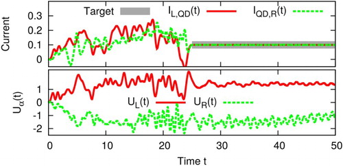
The system has now the freedom to adjust the density and currents from time 0 to such that the target patterns can be reached. There are two ways to achieve a DC current flowing through a Josephson junction:

1. Following Equations (28(28) )–(29(29) ), only the case produces a DC current, namely . This is the DC Josephson effect. In general, this relation is not true for our model, since the quantum dot always supports two Andreev bound states for U=0 [50]. They lead to persistent oscillations in the current and density [50,73,74]. The oscillations in the current can be compensated by small variations of the bias around the origin. Figure 9 shows an example of such a solution. This approach is limited by and hence does not work for arbitrary large DC currents.

2. An alternative approach is to apply a DC bias across the junction, leading to a linear increase in the phase difference and thus to oscillations in the currents. This is the AC Josephson effect. These oscillations can be compensated again by small variations in the bias, the reaction to these changes cancels the Josephson oscillations. Figure 10 shows an example for this type of solutions.

Figure 9. SQDS junction with optimised currents and . We remove the constraint since the target can not be reached otherwise. The target is the same for both currents and starts at t=25. The solution exploits the DC Josephson effect. The parameters are: .

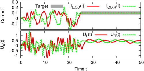
Figure 10. Same junction as in Figure 9, but a different solution to the problem. This solution exploits the AC Josephson effect.

5. Optimising the Cooper pair splitting efficiency

In this section, we demonstrate how to optimise the Cooper pair splitting efficiency in a two-quantum dot Y-junction. The overall idea is to create entangled electrons at two quantum dots.

The entanglement of quantum particles has fascinated the scientific community since the proposition of the Einstein-Podolsky–Rosen (EPR) Gedankenexperiment [75]. Entanglement means that two particles are linked such that the measurement of one particle is sufficient to completely determine the quantum state of the other one. A prominent example is a pair of electrons with opposite spin. Suppose, you have a pair of entangled electron in a spin singlet. Then, one spin is up and the other spin is always pointing downwards. Photons are a second example which can be entangled with respect to the polarisation.

The EPR Gedankenexperiment is directly linked to the question of non-locality of quantum mechanics: Can a measurement at position x have an influence on a simultaneous or later independent measurement at a different position ? This question can be cast into a mathematical formula known as Bell's inequality [76]. A violation of the latter would prove the non-locality of quantum mechanics.

Great progress has been achieved with entangled photons, but the final experiment ruling out all possible loopholes has not yet been accomplished [77]. For example, the two measurements at and have to be separated such that , i.e. no information of the first measurement can be transmitted to the second. Hence large distances are typically required to close this loophole [78]. Another important loophole stems from the detector efficiency, i.e. one has to take into account that undetected particles might behave completely different compared to the detected ones. Typically, one uses the fair sampling assumption stating that the detected particles are selected randomly and behave statistically in the same way as the undetected ones.

To do similar Bell test experiments with electrons is much more difficult and remains an open challenge. In recent years, a number of ingenious experiments to create entangled electrons have been performed [79–82], going along with several theoretical developments [83–88]. The basic idea is to use a superconductor as a source of entangled electrons. In the BCS ground state, electrons form Cooper pairs due to the attractive interaction caused by phonons. These pairs consist of two electrons with opposite spin and momentum.

The idea is to create a splitted Cooper pair at the two quantum dots, i.e. one electron is on the left quantum dot and the other with opposite spin is on the right one (see sketch in Figure 11). However, this process competes with the case of both electrons moving onto the same quantum dot. The latter can be suppressed by a large charging energy of the quantum dots caused by the Coulomb interaction. This make double occupancies less likely.

Figure 11. Sketch of the Y-junction and explanation of all relevant parameters. Only the lead labelled with S is superconducting. The grey colour is used to indicate the superconducting part. The aim is to create entangled electrons on the two quantum dots. All three leads are semi infinite.

We propose a way to achieve splitting efficiencies of and more, which we hope will help the eventual experimental demonstration of the violation of Bell's inequality. In comparison to traditional approaches, our method has two major differences. First, we do not rely on a large Coulomb repulsion on the quantum dots but rather use optimal control theory to tailor the bias in the normal leads in such a way that the splitting probability is maximised. Second, we look at the Cooper pair density on the quantum dots as opposed to the experimental approaches working currents of entangled electrons in the two normal conducting leads. Consequently, a direct comparison of results is not easily possible as the efficiencies measure different ratios. As a future work, it might be worth doing an extensive comparative study answering whether the here created pair eventually moves towards the leads or stays on the quantum dots. In experiments, splitting efficiencies for the current of have been realised in recent experiments [82] being significantly higher than previous results. Despite this progress, the experimental proof of the violation of Bell's inequality is still pending.

In contrast to all systems studied in the previous sections, we now work with three leads. The system is sketched in Figure 11. It consists of two quantum dots ( and ), one superconducting () and two normal leads ( and ).

The Hamiltonian of our modified model reads (32) (33) (34) (35)

Note that there is only a bias in the left and right lead. All parameters are again chosen real and positive. Furthermore, we work at temperature T=0 and assume the wide band limit . Again, only the coupling strengths will be stated.

In the following, we demonstrate how to optimise the Cooper pair splitting efficiency in the above model of a two-quantum dot Y-junction. The goal is to operate the device as a Cooper pair splitter that creates entangled electrons on the two quantum dots. The splitting of a Cooper pair can be understood as a crossed Andreev reflection. An incoming electron in one of the normal leads gets reflected into the other lead as a hole. This creates a Cooper pair in the superconductor. The process is sketched in Figure 12 (top left). Similarly, the opposite process removes a Cooper pair from the superconductor. Besides, there are three other possible reflection processes: (a) normal reflection, (b) Andreev reflection, and (c) elastic cotunnelling. The latter corresponds to a reflection of the incoming electron to the opposite lead. These three processes together with the crossed Andreev reflection are all sketched in Figure  12.

Figure 12. Overview of the four possible reflection processes. Black arrows indicate electrons, white arrows represent holes. The grey block is the superconducting lead of Figure 11. Top left: Sketch of a crossed Andreev reflection. The incoming spin up electron in the left lead gets reflected as a spin down hole to the right lead. Simultaneously, a Cooper pair is created in the superconducting lead. The opposite process, which removes a Cooper pair from the superconductor, is also possible. Bottom left: The reflected hole stays in the left lead. This corresponds to the normal Andreev reflection. Top right: Sketch of an elastic cotunnelling process. Now, the incoming electron gets reflected into the right lead. Bottom right: Alternatively, the electron can also be reflected into the left lead corresponding to normal reflection.

The central ingredient for the optimisation process is the proper definition of a suitable objective function which is then to be maximised. It has to quantify the Cooper pair splitting efficiency. To this end, we first define the so-called pairing density or anomalous density as (36)

We use its absolute value squared as a measure for the Cooper pair density with one electron at and the other at . We propose to maximise the following objective function: (37)

The fraction represents the Cooper pair splitting efficiency at time t, which is expressed as the amount of Cooper pairs being split up divided by the total amount of Cooper pairs on the quantum dots. We calculate its average over the time span from to . The pairing densities are obtained from the single particle wave functions , i.e. the solutions of the time-dependent Bogoliubov–de Gennes equation (7(7) ).

We want to tailor the bias such that we maximise the time averaged Cooper pair splitting efficiency. The corresponding optimisation problem then reads (38)

The problem can be solved using again standard derivative-free algorithms for nonlinear optimisation problems, for example the ones provided by the library NLopt [70].

To achieve high splitting efficiencies it is essential that the junction is asymmetric, i.e. the couplings to the left and to the right quantum dot must not be equal. This is necessary since we observe an upper bound of for the Cooper pair splitting efficiency in symmetric junctions, which is already achieved in the ground state by the usual Cooper pair tunnelling leading to the proximity effect. Hence any optimisation starting in the ground state will not improve the results. The underlying cause for this limitation is still unknown and under investigation. In order to bypass this issue, we choose an asymmetric coupling of the quantum dots to the normal leads.

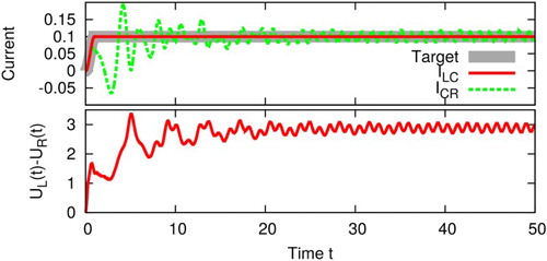
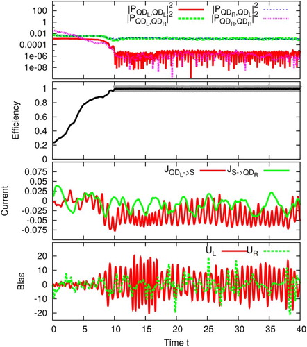
The results of such an optimisation are depicted in Figure 13. The bias is tailored such that the Cooper pair splitting efficiency is maximised. It suppresses the non-splitting processes. The efficiency is optimised in the time interval from to . This interval is indicated by the underlying thick grey line in the plot of the efficiency (second from top). In this interval, we achieve an average efficiency of more than . The values of and are on top of each other. The resulting currents flowing through the junction indicate, that in the time average, there is a net current flowing from the right normal conducting lead (R) via the superconductor (S) to the left one (L). This is deduced from the observation that and are both negative in the time average. We point out, that this does not say anything about the movement of the entangled Cooper pairs.

Figure 13. Simulation with an optimised bias. (a) Top: as a function of time. (b) Second from top: Resulting efficiency, grey line indicates time interval of optimisation. second from bottom (c) Second from bottom: Resulting currents and . (d) Bottom: Tailored bias and of the optimisation. The parameters are: , , , , N=200.

This result clearly demonstrates that the Coulomb interaction at the quantum dots is not necessary in order to obtain high efficiencies. One can also succeed with optimised biases.

6. Conclusion

Usually, in the field of molecular electronics, the goal is to calculate the steady-state or time-dependent current that is generated by a given bias and gate voltage. Sometimes, however, one may be interested in taking a step beyond this point and control the current or other observables of the junction. To this end we have presented an algorithm that allows us to calculate the time-dependent bias that achieves a prescribed goal. In the examples presented, we determine numerically the time-dependent bias that forces the current, the density or the molecular vibration to follow a given temporal pattern. The method is general and not restricted to the observables listed above. In the final section we apply our approach to optimise the Cooper pair splitting efficiency in a Y-junction with two quantum dots. We successfully create spatially separated entangled electron pairs with an efficiency of nearly 100 %. We expect our approach to be useful in the control of other – essentially arbitrary – observables in molecular junctions.

Disclosure statement

No potential conflict of interest was reported by the authors.

References

- A. Aviram and M.A. Ratner, Chem. Phys. Lett. 29 (2), 277 (1974). doi: 10.1016/0009-2614(74)85031-1
- G. Cuniberti, G. Fagas and K. Richter, Introducing Molecular Electronics (Springer, Berlin, 2005).
- M. Di Ventra, Electrical Transport in Nanoscale Systems, 1st ed. (Cambridge University Press, New York, 2008).
- J.C. Cuevas and E. Scheer, Molecular Electronics (World Scientific Publishing Company, Singapore, 2010).
- E. Runge and E.K.U. Gross, Phys. Rev. Lett. 52 (12), 997 (1984). doi: 10.1103/PhysRevLett.52.997
- R. Baer, T. Seideman, S. Ilani and D. Neuhauser, J. Chem. Phys. 120 (7), 3387 (2004). doi: 10.1063/1.1640611
- K. Burke, R. Car and R. Gebauer, Phys. Rev. Lett. 94 (14), 146803 (2005). doi: 10.1103/PhysRevLett.94.146803
- S. Kurth, G. Stefanucci, C.O. Almbladh, A. Rubio and E.K.U. Gross, Phys. Rev. B 72 (3), 035308 (2005). doi: 10.1103/PhysRevB.72.035308
- J. Yuen-Zhou, C. Rodriguez-Rosario and A. Aspuru-Guzik, Phys. Chem. Chem. Phys. 11 (22), 4509 (2009). doi: 10.1039/b903064f
- M. Di Ventra and R. D'Agosta, Phys. Rev. Lett. 98 (22), 226403 (2007). doi: 10.1103/PhysRevLett.98.226403
- H. Appel and M. Di Ventra, Phys. Rev. B 80 (21), 212303 (2009). doi: 10.1103/PhysRevB.80.212303
- H. Appel and M. Di Ventra, Chem. Phys. 391 (1), 27 (2011). doi: 10.1016/j.chemphys.2011.05.001
- G. Stefanucci and R. van Leeuwen, Nonequilibrium Many-Body Theory of Quantum Systems: A Modern Introduction (Cambridge University Press, Cambridge, 2013).
- P. Myöhänen, A. Stan, G. Stefanucci and R. van Leeuwen, Phys. Rev. B 80, 115107 (2009). doi: 10.1103/PhysRevB.80.115107
- P. Myöhänen, A. Stan, G. Stefanucci and R. van Leeuwen, J. Phys. 220 (1), 012017 (2010).
- M. Knap, W. von der Linden and E. Arrigoni, Phys. Rev. B 84 (11), 115145 (2011). doi: 10.1103/PhysRevB.84.115145
- J. Zanghellini, M. Kitzler, T. Brabec and A. Scrinzi, J. Phys. B 37 (4), 763 (2004). doi: 10.1088/0953-4075/37/4/004
- H. Wang and M. Thoss, J. Chem. Phys. 131 (2), 024114 (2009). doi: 10.1063/1.3173823
- H. Wang and M. Thoss, J. Phys. Chem. A 117 (32), 7431 (2013). doi: 10.1021/jp401464b
- K.F. Albrecht, H. Wang, L. Mühlbacher, M. Thoss and A. Komnik, Phys. Rev. B 86, 081412 (2012). doi: 10.1103/PhysRevB.86.081412
- L. Mühlbacher and E. Rabani, Phys. Rev. Lett. 100 (17), 176403 (2008). doi: 10.1103/PhysRevLett.100.176403
- Y. Wang, C.Y. Yam, T. Frauenheim, G.H. Chen and T.A. Niehaus, Chem. Phys. 391 (1), 69 (2011). doi: 10.1016/j.chemphys.2011.04.006
- Y. Zhang, S. Chen and G.H. Chen, Phys. Rev. B 87 (8), 085110 (2013).
- C. Oppenländer, B. Korff, T. Frauenheim and T.A. Niehaus, Phys. Status Solidi B 250 (11), 2349 (2013). doi: 10.1002/pssb.201349162
- J. Jin, X. Zheng and Y. Yan, J. Chem. Phys. 128 (23), 234703 (2008). doi: 10.1063/1.2938087
- X. Zheng, J. Jin and Y. Yan, New. J. Phys. 10 (9), 093016 (2008). doi: 10.1088/1367-2630/10/9/093016
- X. Zheng, J. Jin and Y. Yan, J. Chem. Phys. 129 (18), 184112 (2008). doi: 10.1063/1.3010886
- L. Pontryagin, V.G. Boltyanskii, R.V. Gamkrelidze and E.F. Mischenko, Mathematical Theory of Optimal Processes (John Wiley & Sons, New York, 1962).
- R. Bellman, Dynamic Programming (Princeton University Press, Princeton, NJ, 1957).
- A.P. Peirce, M.A. Dahleh and H. Rabitz, Phys. Rev. A 37, 4950 (1988). doi: 10.1103/PhysRevA.37.4950
- S. Shi, A. Woody and H. Rabitz, J. Chem. Phys. 88 (11), 6870 (1988). doi: 10.1063/1.454384
- R. Kosloff, S. Rice, P. Gaspard, S. Tersigni and D. Tannor, Chem. Phys. 139 (1), 201 (1989). doi: 10.1016/0301-0104(89)90012-8
- I. Serban, J. Werschnik and E.K.U. Gross, Phys. Rev. A 71, 053810 (2005). doi: 10.1103/PhysRevA.71.053810
- E. Räsänen, A. Castro, J. Werschnik, A. Rubio and E.K.U. Gross, Phys. Rev. Lett. 98, 157404 (2007). doi: 10.1103/PhysRevLett.98.157404
- J. Werschnik and E.K.U. Gross, J. Phys, B 40 (18), R175 (2007). doi: 10.1088/0953-4075/40/18/R01
- A. Assion, T. Baumert, M. Bergt, T. Brixner, B. Kiefer, V. Seyfried, M. Strehle and G. Gerber, Science 282 (5390), 919 (1998). doi: 10.1126/science.282.5390.919
- B. Hartke, J. Manz and J. Mathis, Chem. Phys. 139, 123 (1989). doi: 10.1016/0301-0104(89)90007-4
- N. Elghobashi, P. Krause, J. Manz and M. Oppel, Phys. Chem. Chem. Phys. 5, 4806 (2003). doi: 10.1039/B305305A
- N. Elghobashi and L. Gonzalez, Phys. Chem. Chem. Phys. 6, 4071 (2004). doi: 10.1039/B409446H
- R.J. Levis, G.M. Menkir and H. Rabitz, Science 292 (5517), 709 (2001). doi: 10.1126/science.1059133
- D.M. Reich and C.P. Koch, New. J. Phys. 15 (12), 125028 (2013). doi: 10.1088/1367-2630/15/12/125028
- E. Räsänen, T. Blasi, M.F. Borunda and E.J. Heller, Phys. Rev. B 86, 205308 (2012). doi: 10.1103/PhysRevB.86.205308
- E. Räsänen and E.J. Heller, Eur. Phys. J. B 86 (1), 17 (2013). doi: 10.1140/epjb/e2012-30921-4
- A. Castro, E. Räsänen, A. Rubio and E.K.U. Gross, EPL (Europhysics Letters) p. 53001 (2009).
- E. Räsänen and L.B. Madsen, Phys. Rev. A 86, 033426 (2012). doi: 10.1103/PhysRevA.86.033426
- W. Jakubetz, J. Manz and H.J. Schreier, Chem. Phys. Lett. 165 (1), 100 (1990). doi: 10.1016/0009-2614(90)87018-M
- G.Q. Li, M. Schreiber and U. Kleinekathöfer, EPL (Europhysics Letters) p. 27006 (2007).
- A.F. Amin, G.Q. Li, A.H. Phillips and U. Kleinekathöfer, Eur. Phys. J B 68 (1), 103 (2009). doi: 10.1140/epjb/e2009-00075-9
- G.Q. Li and U. Kleinekathöfer, Eur. Phys. J. B 76 (2), 309 (2010). doi: 10.1140/epjb/e2010-00206-3
- G. Stefanucci, E. Perfetto and M. Cini, Phys. Rev. B 81 (11), 115446 (2010). doi: 10.1103/PhysRevB.81.115446
- M. Galperin, M.A. Ratner and A. Nitzan, J. Phys. 19 (10), 103201 (2007).
- J. Koch and F. von Oppen, Phys. Rev. Lett. 94, 206804 (2005).
- D.A. Ryndyk, M. Hartung and G. Cuniberti, Phys. Rev. B 73, 045420 (2006). doi: 10.1103/PhysRevB.73.045420
- R. Härtle, C. Benesch and M. Thoss, Phys. Rev. Lett. 102, 146801 (2009). doi: 10.1103/PhysRevLett.102.146801
- C. Verdozzi, G. Stefanucci and C.O. Almbladh, Phys. Rev. Lett. 97 (4), 046603 (2006). doi: 10.1103/PhysRevLett.97.046603
- M. Galperin, M.A. Ratner and A. Nitzan, Nano Lett. 5 (1), 125 (2004). doi: 10.1021/nl048216c
- M. Galperin, A. Nitzan and M.A. Ratner, J. Phys. 20 (37), 374107 (2008).
- G. Li, B. Movaghar, A. Nitzan and M.A. Ratner, J. Chem. Phys. 138 (4), 044112 (2013). doi: 10.1063/1.4776230
- K.J. Franke and J.I. Pascual, J. Phys. 24 (39), 394002 (2012).
- W. Zhu, J. Botina and H. Rabitz, J. Chem. Phys. 108 (5), 1953 (1998). doi: 10.1063/1.475576
- S.E. Sklarz and D.J. Tannor, Phys. Rev. A 66 (5), 053619 (2002).
- J.P. Palao and R. Kosloff, Phys. Rev. A 68 (6), 062308 (2003). doi: 10.1103/PhysRevA.68.062308
- K. Krieger, A. Castro and E.K.U. Gross, Chem. Phys. 391 (1), 50 (2011). doi: 10.1016/j.chemphys.2011.04.014
- M. Hellgren, E. Räsänen and E.K.U. Gross, Phys. Rev. A 88 (1), 013414 (2013). doi: 10.1103/PhysRevA.88.013414
- E. Räsänen, A. Putaja and Y. Mardoukhi, Cent. Eur. J. Phys. 11 (9), 1066 (2013).
- R.S. Judson and H. Rabitz, Phys. Rev. Lett. 68 (10), 1500 (1992). doi: 10.1103/PhysRevLett.68.1500
- M.J.D. Powell, Department of Applied Mathematics and Theoretical Physics, Cambridge England, technical report NA2009/06 (2009).
- M.J.D. Powell, in Advances in Optimization and Numerical Analysis, edited by Susana Gomez and Jean-Pierre Hennart (Springer, Dordrecht, 1994), Vol. 275, pp. 51–67.
- M.J.D. Powell, Acta Numerica 7, 287 (1998). doi: 10.1017/S0962492900002841
- S.G. Johnson, The NLopt nonlinear-optimization package <url: http://ab-initio.mit.edu/nlopt>, 2013.
- A. Castro and E. Gross, J. Phys. A 47 (2), 025204 (2014). doi: 10.1088/1751-8113/47/2/025204
- B.D. Josephson, Phys. Lett. 1 (7), 251 (1962). doi: 10.1016/0031-9163(62)91369-0
- G. Stefanucci, Phys. Rev. B 75 (19), 195115 (2007). doi: 10.1103/PhysRevB.75.195115
- E. Khosravi, S. Kurth, G. Stefanucci and E.K.U. Gross, Appl. Phys. A 93 (2), 355 (2008). doi: 10.1007/s00339-008-4864-9
- A. Einstein, B. Podolsky and N. Rosen, Phys. Rev. 47 (10), 777 (1935). doi: 10.1103/PhysRev.47.777
- J.S. Bell, Physics 1, 195 (1964). doi: 10.1103/PhysicsPhysiqueFizika.1.195
- M. Giustina, A. Mech, S. Ramelow, B. Wittmann, J. Kofler, J. Beyer, A. Lita, B. Calkins, T. Gerrits, S.W. Nam, R. Ursin and A. Zeilinger, Nature 497 (7448), 227 (2013). doi: 10.1038/nature12012
- G. Weihs, T. Jennewein, C. Simon, H. Weinfurter and A. Zeilinger, Phys. Rev. Lett. 81 (23), 5039 (1998). doi: 10.1103/PhysRevLett.81.5039
- L. Hofstetter, S. Csonka, J. Nygard and C. Schönenberger, Nature 461 (7266), 960 (2009). doi: 10.1038/nature08432
- L. Hofstetter, S. Csonka, A. Baumgartner, G. Fülöp, S. d'Hollosy, J. Nygård and C. Schönenberger, Phys. Rev. Lett. 107 (13), 136801 (2011). doi: 10.1103/PhysRevLett.107.136801
- L.G. Herrmann, F. Portier, P. Roche, A. Levy Yeyati, T. Kontos and C. Strunk, Phys. Rev. Lett. 104 (2), 026801 (2010). doi: 10.1103/PhysRevLett.104.026801
- J. Schindele, A. Baumgartner and C. Schönenberger, Phys. Rev. Lett. 109, 157002 (2012). doi: 10.1103/PhysRevLett.109.157002
- P. Recher, E.V. Sukhorukov and D. Loss, Phys. Rev. B 63, 165314 (2001). doi: 10.1103/PhysRevB.63.165314
- P. Recher and D. Loss, J. Superconductivity 15 (1), 49 (2002). doi: 10.1023/A:1014027227087
- O. Sauret, D. Feinberg and T. Martin, Phys. Rev. B 70 (24), 245313 (2004). doi: 10.1103/PhysRevB.70.245313
- J.P. Morten, A. Brataas and W. Belzig, Phys. Rev. B 74, 214510 (2006). doi: 10.1103/PhysRevB.74.214510
- D.S. Golubev and A.D. Zaikin, Phys. Rev. B 76, 184510 (2007). doi: 10.1103/PhysRevB.76.184510
- P. Burset, W.J. Herrera and A. Levy Yeyati, Phys. Rev. B 84 (11), 115448 (2011). doi: 10.1103/PhysRevB.84.115448