Pre-Born–Oppenheimer molecular structure theory

ABSTRACT

In pre-Born–Oppenheimer (pre-BO) theory a molecule is considered as a quantum system as a whole, including the electrons and the atomic nuclei on the same footing. This approach is fundamentally different from the traditional quantum chemistry treatment, which relies on the separation of the motion of the electrons and the atomic nuclei. A fully quantum mechanical description of molecules has a great promise for future developments and applications. Its most accurate versions may contribute to the definition of new schemes for metrology and testing fundamental physical theories; its approximate versions can provide an efficient theoretical description for molecule-positron interactions and, in general, it would circumvent the tedious computation and fitting of potential energy surfaces and non-adiabatic coupling vectors while it includes also the quantum nuclear motion also often called ‘molecular quantum dynamics’. To achieve these goals, the review points out important technical and fundamental open questions. Most interestingly, the reconciliation of pre-BO theory with the classical chemistry knowledge touches upon fundamental problems related to the measurement problem of quantum mechanics.

GRAPHICAL ABSTRACT

Keywords:

• pre-Born–Oppenheimer theory
• molecular structure in quantum mechanics
• rovibronic resonances
• explicitly correlated Gaussian functions
• stochastic variational method

1. Quantum chemistry vs. quantum mechanics and chemistry?

We start this article with a historical overview of the chemical theory of molecular structure and the origins of quantum chemistry, which is followed by methodological details and applications of pre-Born–Oppenheimer theory.

1.1. Historical background: chemical structure, physical structure from organic chemistry experiments

[T]he dominating story in chemistry of the 1860s, 1870s, and 1880s was neither the periodic law, nor the search for new elements, nor the early stages of the study of atoms and molecules as physical entities. It was the maturation, and demonstration of extraordinary scientific and technological power, of the “theory of chemical structure”…

Alan J. Rocke

Image and Reality: Kekulé, Kopp, and the Scientific

Imagination

(The University of Chicago Press, Chicago and London, 2010)

During the second half of the 19th century, the pioneering organic chemists generation—represented by Williamson, Kekulé, Butlerov, Crum Brown, Frankland, and Wurtz—had explored an increasing number of chemical transformations in their laboratory experiments and worked towards the establishment of a logical framework for their observations. The ‘first chemistry conference’, held in Karlsruhe on 3 September 1860, resulted in an internationally recognised definition of the atomic masses. This agreement ensured that the same molecular formula was then used for the same substance in all laboratories around the world, and thereby opened the route to the successful development of the theory of chemical structure. The development of the chemical theory had been surrounded by heated debates about what was reality and what was mere speculation. Contemporary physics (gravitation, electromagnetism) was not able to provide any satisfactory description for molecules. To give a taste of this exciting period, we reproduce a few extracts from Alan J. Rocke's chemical history book [1]:

• Friedrich August Kekulé [von Stradonitz] (1858): ‘rational formulas are reaction formulas, and can be nothing more in the current state of science’.

• Friedrich August Kekulé [von Stradonitz] (1859): ‘[he] rejected the possibility of determining the physical arrangement of the constituent atoms in a molecule from the study of chemical reactions, since chemical reactions necessarily alter the arrangements of the atoms in the molecule’.

• Charles Adolphe Wurtz (1860): ‘[W]e do not have any means of assuring ourselves in an absolute manner of the arrangement, or even the real existence of the groups which appear in our rational formulas…merely express parental ties’.

• Hermann Kolbe (1866): ‘Frankly, I consider all these graphical representations…as dangerous, because the imagination is thereby given too free rein’.

• Johannes Wislicenus (1869): ‘[it] must somehow be explained by the different arrangements of their atoms in space’.

• Jacobus Henricus van't Hoff (5 September 1874, 1875): ‘La chimie dans l'espace’

• Joseph Achille Le Bel (5 November 1874): physical structure in the 3-dimensional space

1.2. Historical background: application of quantum theory to molecules

At the time when Erwin Schrödinger wrote down his famous wave equation [2], the concept of the classical skeleton of the atomic nuclei arranged in the three-dimensional space was already a central idea in molecular science derived from the organic chemists' laboratory experiments. The idea of a separate description of the electrons and the atomic nuclei, i.e. the motion of the atomic nuclei on a potential energy surface (PES), which results form the solution of the electronic problem in the field of fixed external nuclear charges, is usually connected to the work of Born and Oppenheimer in 1927 [3] and perhaps the later references [4,5] are also cited. At the same time, Sutcliffe and Woolley analyze in reference [6] René Marcelin's doctoral dissertation published in 1914 (the author died during World War I), which appears to be the earliest work in which ideas reminiscent of a potential energy surface can be found. Sutcliffe and Woolley argue that the idea of clamping the atomic nuclei in order to define an electronic problem was attempted already within the framework of The Old Quantum Theory, and later these attempts were taken over (more successfully) to Schrödinger's theory for molecules. In any case, what we usually mean by quantum chemistry gains its equations from a combination of quantum mechanics and the Born–Oppenheimer (BO) approximation (and perhaps corrections to the BO approximation are also included).

1.3. Quantum chemistry

The tremendous success of the usual practice might perhaps be best regarded as a tribute to the insight and ingenuity of the practitioners for inventing an effective variant of quantum theory for chemistry.

B. T. Sutcliffe and R. G. Woolley, J. Chem. Phys. 137,

22A544 (2012) [7].

The well-known theory applicable to molecules has grown out from the separation of the motion of the electrons and the atomic nuclei. This separation defines two major fields for quantum chemistry, electronic structure theory and the corresponding electronic Hamiltonian (in atomic units): (1) $\begin{array}{rl}{\hat{H}}_{\mathrm{el}}& =-\sum _{i=1}^{n_{\mathrm{e}}}\frac{1}{2}{\mathrm{\Delta }}_{{\mathbf{r}}_i}+\sum _{i=1}^{n_{\mathrm{e}}}\sum _{j>i}^{n_{\mathrm{e}}}\frac{1}{|{\mathbf{r}}_i-{\mathbf{r}}_j|}\\ & -\sum _{i=1}^{n_{\mathrm{e}}}\sum _{n=1}^{n_{\mathrm{n}}}\frac{Z_n}{|{\mathbf{r}}_i-{\mathbf{R}}_n|}+\sum _{n=1}^{n_{\mathrm{n}}}\sum _{m>n}^{n_{\mathrm{n}}}\frac{Z_n{Z}_m}{|{\mathbf{R}}_n-{\mathbf{R}}_m|}\end{array}$(1) with the ${\mathbf{r}}_i$ electronic and ${\mathbf{R}}_n$ nuclear positions and electric charges, $Z_n$; and nuclear motion theory with the Hamiltonian for the motion of the atomic nuclei (or rovibrational Hamiltonian): (2) ${\hat{H}}_{\mathrm{nuc}}=\hat{T}\left(\rho \right)+\hat{V},$(2) where $\hat{T}\left(\rho \right)$ is the rovibrational kinetic energy operator and the potential energy, $\hat{V}$, which is called the potential energy surface and it is obtained from the eigenvalues of Equation (1(1) $\begin{array}{rl}{\hat{H}}_{\mathrm{el}}& =-\sum _{i=1}^{n_{\mathrm{e}}}\frac{1}{2}{\mathrm{\Delta }}_{{\mathbf{r}}_i}+\sum _{i=1}^{n_{\mathrm{e}}}\sum _{j>i}^{n_{\mathrm{e}}}\frac{1}{|{\mathbf{r}}_i-{\mathbf{r}}_j|}\\ & -\sum _{i=1}^{n_{\mathrm{e}}}\sum _{n=1}^{n_{\mathrm{n}}}\frac{Z_n}{|{\mathbf{r}}_i-{\mathbf{R}}_n|}+\sum _{n=1}^{n_{\mathrm{n}}}\sum _{m>n}^{n_{\mathrm{n}}}\frac{Z_n{Z}_m}{|{\mathbf{R}}_n-{\mathbf{R}}_m|}\end{array}$(1) ) computed at different positions of the atomic nuclei.

Within this framework, a variety of molecular properties are derived from the eigenstates of the electronic Hamiltonian, Equation (1(1) $\begin{array}{rl}{\hat{H}}_{\mathrm{el}}& =-\sum _{i=1}^{n_{\mathrm{e}}}\frac{1}{2}{\mathrm{\Delta }}_{{\mathbf{r}}_i}+\sum _{i=1}^{n_{\mathrm{e}}}\sum _{j>i}^{n_{\mathrm{e}}}\frac{1}{|{\mathbf{r}}_i-{\mathbf{r}}_j|}\\ & -\sum _{i=1}^{n_{\mathrm{e}}}\sum _{n=1}^{n_{\mathrm{n}}}\frac{Z_n}{|{\mathbf{r}}_i-{\mathbf{R}}_n|}+\sum _{n=1}^{n_{\mathrm{n}}}\sum _{m>n}^{n_{\mathrm{n}}}\frac{Z_n{Z}_m}{|{\mathbf{R}}_n-{\mathbf{R}}_m|}\end{array}$(1) ), and an effective combination of the quantum mechanics of electrons with classical electronic properties of identifiable nuclei and quantum mechanics for nuclear motions, Equation (2(2) ${\hat{H}}_{\mathrm{nuc}}=\hat{T}\left(\rho \right)+\hat{V},$(2) ).

Several chemical concepts gain a theoretical background from this construct, most importantly the potential energy surface (PES) is defined. Its minimum structure (or structures if it has several local minima) defines the equilibrium structure, which is a purely mathematical construct resulting from the separability approximation but it is usually identified with the classical molecular structure. Then, the nuclei are re-quantised to solve the Schrödinger equation of the atomic nuclei, Equation (2(2) ${\hat{H}}_{\mathrm{nuc}}=\hat{T}\left(\rho \right)+\hat{V},$(2) ), to calculate rovibrational states, resonances, reaction rates, etc.

The electronic structure and quantum nuclear motion theories have many similar features but each field have its own peculiarities. Most importantly, the spatial symmetries are different: in electronic-structure theory the point-group symmetry is defined by the fixed, classical nuclear skeleton, whereas in nuclear-motion theory the PES depends only on the relative positions of the nuclei in agreement with the translational and rotational invariance of an isolated molecule. Furthermore in electronic-structure theory, the molecular translations and rotations are separated off by fixing the atomic nuclei, and thus the kinetic energy can be written in a very simple form in Cartesian coordinates. In nuclear-motion theory, it is convenient to define a frame fixed to the (non-rigid) body to separate off the translation and to account for the spatial orientation of this frame by three angles [8, 9]. Thereby, in a usual nuclear-motion theory treatment, the coordinates are necessarily curvilinear. In spite of all complications, it was possible to develop automated procedures [10–14], which allow us to efficiently compute hundreds or thousands of rovibrational energy states for small molecules using curvilinear coordinates appropriately chosen for a molecular system [15–17].

1.4. Quantum mechanics and chemistry?

The direct treatment of molecules as few-particle quantum systems is much less explored. Nevertheless, we may think about a molecule as a quantum system as a whole without any a priori separation of the particles, which we call pre-Born–Oppenheimer (pre-BO) molecular structure theory (it is also called non-Born–Oppenheimer theory in the literature [18,19]).

The $(n_{\mathrm{p}}+1)$-particle time-independent Schrödinger equation (3) $\hat{H}\mathrm{\Psi }=E\mathrm{\Psi }$(3) contains the non-relativistic Hamiltonian (4) $\hat{H}=\hat{T}+\hat{V},$(4) which is the sum of the kinetic energy operator (5) $\hat{T}=-\sum _{i=1}^{n_{\mathrm{p}}+1}\frac{1}{2m_i}{\mathrm{\Delta }}_{{\mathbf{r}}_i}$(5) and the Coulomb potential energy operator (6) $\hat{V}=\sum _{i=1}^{n_{\mathrm{p}}+1}\sum _{j>i}^{n_{\mathrm{p}}+1}\frac{q_i{q}_j}{|{\mathbf{r}}_i-{\mathbf{r}}_j|},$(6) where atomic units are used and ${\mathbf{r}}_i$ labels the laboratory-fixed (LF) Cartesian coordinates of the ith particle. The full molecular Hamiltonian has $2(n_{\mathrm{p}}+1)$ parameters, the mass and the electric charge for each particle, $m_i$ and $q_i(i=1,2,\dots ,n_{\mathrm{p}}+1)$, respectively. In addition, the physical solutions must satisfy the spin-statistics theorem, thereby the spins $s_i(i=1,2,\dots ,n_{\mathrm{p}}+1)$ (the fermionic or bosonic character) appear as additional parameters. In total, there are $3(n_{\mathrm{p}}+1)$ parameters, which define the molecular system. In addition, we may specify the quantum numbers corresponding to the conserved quantities of an isolated molecule: the total angular momentum, its projection to a space-fixed axis, the parity, and the spin quantum numbers labelled with N, $N_z$, p, $S_a$, $M_{S_a}$, $S_b$, $M_{S_b}$, … (for particle types a, b, etc.), respectively.¹

It is important to note that the full molecular Hamiltonian, $\hat{H}$ specified in Equations (4(4) $\hat{H}=\hat{T}+\hat{V},$(4) )–(6(6) $\hat{V}=\sum _{i=1}^{n_{\mathrm{p}}+1}\sum _{j>i}^{n_{\mathrm{p}}+1}\frac{q_i{q}_j}{|{\mathbf{r}}_i-{\mathbf{r}}_j|},$(6) ), has very different mathematical properties from the electronic Hamiltonian, ${\hat{H}}_{\mathrm{el}}$ in Equation (1(1) $\begin{array}{rl}{\hat{H}}_{\mathrm{el}}& =-\sum _{i=1}^{n_{\mathrm{e}}}\frac{1}{2}{\mathrm{\Delta }}_{{\mathbf{r}}_i}+\sum _{i=1}^{n_{\mathrm{e}}}\sum _{j>i}^{n_{\mathrm{e}}}\frac{1}{|{\mathbf{r}}_i-{\mathbf{r}}_j|}\\ & -\sum _{i=1}^{n_{\mathrm{e}}}\sum _{n=1}^{n_{\mathrm{n}}}\frac{Z_n}{|{\mathbf{r}}_i-{\mathbf{R}}_n|}+\sum _{n=1}^{n_{\mathrm{n}}}\sum _{m>n}^{n_{\mathrm{n}}}\frac{Z_n{Z}_m}{|{\mathbf{R}}_n-{\mathbf{R}}_m|}\end{array}$(1) ). Although the potential energy is the simple Coulomb interaction term both in $\hat{H}$ and ${\hat{H}}_{\mathrm{el}}$, in $\hat{H}$ all electric charges belong to the quantum system. While, for a neutral molecule ${\hat{H}}_{\mathrm{el}}$ has an infinite discrete spectrum and the continuous spectrum begins at the first ionisation energy, the $\hat{H}$ molecular Hamiltonian does not have any discrete spectrum at all unless the overall molecular translation is removed (see for example Refs. [20–22]). In fact, $\hat{H}$ has the same spatial symmetries as ${\hat{H}}_{\mathrm{nuc}}$ in nuclear-motion theory. If we separate off the overall translation of the molecule, the translationally invariant molecular Hamiltonian may or may not have any discrete states, if it has, they end at the lowest dissociation threshold, which is generally unknown (see Section 2.7 and Figure 2).

Figure 1. Example translationally invariant coordinates: coordinates of relative vectors within the many-particle system.

Figure 2. The ladder structure of the pre-Born–Oppenheimer (pre-BO) energy levels is visualised in the right. The left of the figure shows the rovibrational states corresponding to their respective potential energy surfaces in the Born–Oppenheimer (BO) approximation. While in the BO picture, the rovibrational states corresponding to the excited electronic state are bound states, the corresponding rovibronic states in pre-BO theory appear as resonances. [Reprinted with permission from E. Mátyus, J. Phys. Chem. A 117, 7195 (2013). Copyright 2013 American Chemical Society.]

One can introduce new coordinates in $\hat{H}$, in order to (a) separate off the overall translational motion, and (b) to describe the internal dynamics more efficiently. The choice of the coordinates (for the kinetic energy operator) is a question of convenience. We could use some appropriate curvilinear system similarly to nuclear-motion theory. The motivation however for using laboratory-fixed Cartesian coordinates, similarly as in electronic structure theory, is provided by the aim to develop a generally applicable theoretical and computational framework, similarly to the recent electron-nuclear orbital theories [23–30], which have grown out from electronic-structure theory by incorporating (some of the) atomic nuclei in the quantum treatment. Furthermore, (laboratory-fixed) Cartesian coordinates will be the preferred choice for a generalisation to the relativistic regime.

Various direct and highly specialised techniques have been proposed in the literature [31–34] for the solution of the many-particle Schrödinger equation, Equation (4(4) $\hat{H}=\hat{T}+\hat{V},$(4) ). Our approach, a variational solution method using explicitly correlated Gaussian basis functions (ECGs), is detailed in Section 2. ECGs [35,36] have been successfully used in electronic-structure theory [37] and their application for molecules and in general for few-particle quantum systems has been pioneered by Adamowicz and co-workers [18,19] and Suzuki and Varga [38]. An important year in the development of this field is 1993 when Kinghorn and Poshusta [39] and Kozlowski and Adamowicz [40] published tightly converged ECG-variational results for zero total angular momentum states of the Ps${}_2=\{{\mathrm{e}}^{+},{\mathrm{e}}^{+},{\mathrm{e}}^{-},{\mathrm{e}}^{-}\}$, which can be thought of as a ‘quasi molecule’. Later, analytic energy gradients were derived and implemented [41] to speed up the ECG-exponent optimisation, and this development resulted in a highly efficient approach for the computation of ‘real’ diatomic molecules [42,43]. The computational procedures developed by Adamowicz and co-workers have been recently extended to N=1 and N=2 total angular momentum quantum numbers (corresponding to natural parity) [44–47].

The diatomic formalism has been extended also to triatomic molecules in Ref. [48]. Practical computations have been carried out using another generally applicable basis set, in which the ECGs can have complex-valued parameters [49,50]. Computations with complex ECG basis functions are presently considered as a promising, practical generalisation towards polyatomic molecules.

Considerable effort has been devoted by Adamowicz and co-workers for the development and evaluation of leading relativistic corrections, the Darwin and mass-velocity terms, computed as expectation values with the non-Born–Oppenheimer wave functions. The original implementation [51] in 2006 was followed by several applications for ground and vibrationally excited states of diatomic molecules [52–57]. The largest diatomic molecule to date for which the ground-state non-Born–Oppenheimer energy (as well as leading relativistic corrections) were computed is the BH molecule including two nuclei and six electrons on the same footing in the quantum mechanical treatment [58].

Suzuki and Varga pioneered the development of flexible basis sets and their applications with the stochastic variational method for many-particle quantum systems with various spatial symmetries and the elegant derivation of the corresponding integral expressions [59–61]. Their formalism was successfully used for the computation of bound, resonance, and scattering states of positronium and excitonic complexes [62–69] with various quantum numbers.

2. Variational solution of the electron-nuclear Schrödinger equation with explicitly correlated Gaussian functions

A general $(n_{\mathrm{p}}+1)$-particle variational approach, which we call QUANTEN (QUANTum mechanical treatment of Electrons and atomic Nuclei), was developed in Refs. [20,70] for the solution of the time-independent many-particle Schrödinger equation, Equation (3(3) $\hat{H}\mathrm{\Psi }=E\mathrm{\Psi }$(3) ), to obtain (absolute) molecular energies beyond spectroscopic accuracy² corresponding to various non-relativistic quantum numbers, $N,N_z,p,S_a,M_{S_a},S_b,M_{S_b},\dots$. Our aim was to avoid any a priori separation of the different particles, and thus the computational method is applicable over the entire physically allowed range of the $3(n_{\mathrm{p}}+1)$ physical parameters: the $m_i$ mass, the $q_i$ electric charge, and the $s_i$ spin (bosonic or fermionic character) of the particles ($i=1,\dots ,n_{\mathrm{p}}+1$). Details of the variational procedure are reviewed in the next subsections according to the following aspects:

1. Coordinates: translationally invariant (TI) or laboratory-fixed (LF) Cartesian coordinates

2. Hamiltonian: TI and LF forms of the Hamiltonian

3. Basis functions: ECGs with a polynomial prefactor and adapted to the spatial symmetries

4. Matrix elements: analytic expressions with quasi-normalisation and pre-computed quantities using infinite-precision arithmetics

5. Eigensolver: direct diagonalisation using LA-PACK library routines, non-orthogonal basis sets, numerical treatment of near-linear dependencies

6. Parameterisation of the basis functions: the enlargement and refinement of the basis set with one function at a time, fast eigenvalue estimator, sampling-importance resampling, random walk or Powell's method for the refinement of the basis functions

2.1. Coordinates

Translationally invariant (TI) and centre-of-mass (CM) coordinates are obtained from the LF Cartesian coordinates, $\mathbf{r}$, by a linear transformation (7) $\left(\begin{array}{c}\mathbf{x}\\ {\mathbf{R}}_{\mathrm{CM}}\end{array}\right)=(\mathbf{U}\otimes {\mathbf{I}}_3)\mathbf{r}\iff \mathbf{r}=({\mathbf{U}}^{-1}\otimes {\mathbf{I}}_3)\left(\begin{array}{c}\mathbf{x}\\ {\mathbf{R}}_{\mathrm{CM}}\end{array}\right),$(7) where ${\mathbf{R}}_{\mathrm{CM}}$ labels the centre-of-mass coordinates and $\mathbf{x}$ is invariant upon the overall translation of the system, if the constant matrix, $\mathbf{U}\in {\mathbb{R}}^{(n_{\mathrm{p}}+1)\times (n_{\mathrm{p}}+1)}$, has the following properties: (8) $\begin{array}{rl}& \sum _{j=1}^{n_{\mathrm{p}}+1}{U}_{ij}=0,i=1,\dots ,n_{\mathrm{p}}\mathrm{and}\\ & U_{n_{\mathrm{p}}+1,j}=m_j/m_{\mathrm{tot}},j=1,\dots ,n_{\mathrm{p}}+1.\end{array}$(8) (${\mathbf{I}}_3$ denotes the $3\times 3$ dimensional unit matrix). There are infinitely many possible TI coordinate sets (examples are shown in Figure 1), any two of them, $\mathbf{x}$ and $\mathbf{y}$, are related by a linear transformation: (9) $\begin{array}{rl}\left(\begin{array}{c}\mathbf{y}\\ {\mathbf{R}}_{\mathrm{CM}}\end{array}\right)& =(\mathbf{V}{\mathbf{U}}^{-1}\otimes {\mathbf{I}}_3)\left(\begin{array}{c}\mathbf{x}\\ {\mathbf{R}}_{\mathrm{CM}}\end{array}\right)\iff \left(\begin{array}{c}\mathbf{x}\\ {\mathbf{R}}_{\mathrm{CM}}\end{array}\right)\\ & =(\mathbf{U}{\mathbf{V}}^{-1}\otimes {\mathbf{I}}_3)\left(\begin{array}{c}\mathbf{y}\\ {\mathbf{R}}_{\mathrm{CM}}\end{array}\right)\end{array}$(9) with (10) $\left(\begin{array}{c}\mathbf{y}\\ {\mathbf{R}}_{\mathrm{CM}}\end{array}\right)=(\mathbf{V}\otimes {\mathbf{I}}_3)\mathbf{r}\iff \mathbf{r}=({\mathbf{V}}^{-1}\otimes {\mathbf{I}}_3)\left(\begin{array}{c}\mathbf{y}\\ {\mathbf{R}}_{\mathrm{CM}}\end{array}\right),$(10) where $\mathbf{V}$ satisfies the same conditions as $\mathbf{U}$ in Equation (8(8) $\begin{array}{rl}& \sum _{j=1}^{n_{\mathrm{p}}+1}{U}_{ij}=0,i=1,\dots ,n_{\mathrm{p}}\mathrm{and}\\ & U_{n_{\mathrm{p}}+1,j}=m_j/m_{\mathrm{tot}},j=1,\dots ,n_{\mathrm{p}}+1.\end{array}$(8) ).

2.2. Hamiltonian

Translationally invariant energies and wave functions are computed from a translationally invariant Hamiltonian [20], which is obtained from writing the kinetic energy operator in TI Cartesian coordinates, defined in Equations (7(7) $\left(\begin{array}{c}\mathbf{x}\\ {\mathbf{R}}_{\mathrm{CM}}\end{array}\right)=(\mathbf{U}\otimes {\mathbf{I}}_3)\mathbf{r}\iff \mathbf{r}=({\mathbf{U}}^{-1}\otimes {\mathbf{I}}_3)\left(\begin{array}{c}\mathbf{x}\\ {\mathbf{R}}_{\mathrm{CM}}\end{array}\right),$(7) ) and (8(8) $\begin{array}{rl}& \sum _{j=1}^{n_{\mathrm{p}}+1}{U}_{ij}=0,i=1,\dots ,n_{\mathrm{p}}\mathrm{and}\\ & U_{n_{\mathrm{p}}+1,j}=m_j/m_{\mathrm{tot}},j=1,\dots ,n_{\mathrm{p}}+1.\end{array}$(8) ), and by subtracting the kinetic energy operator of the centre of mass. An alternative approach has been proposed in Refs. [22,71], which avoids any transformation of the operators and eliminates the translational contamination from the matrix elements of the $(n_{\mathrm{p}}+1)$-particle kinetic energy operator, Equation (5(5) $\hat{T}=-\sum _{i=1}^{n_{\mathrm{p}}+1}\frac{1}{2m_i}{\mathrm{\Delta }}_{{\mathbf{r}}_i}$(5) ), during the course of the integral evaluation.

2.3. Basis functions

We approximate an eigenfunction corresponding to some spatial $\lambda =\left(N{M}_{N}p\right)$ and spin $\varsigma =(S_a,M_{S_a},S_b,M_{S_b},\dots )$ quantum numbers as a linear combination of symmetry-adapted basis functions (11) ${\mathrm{\Psi }}^{[\lambda ,\varsigma ]}=\sum _{I=1}^{N_{\mathrm{b}}}{c}_I{\mathrm{\Phi }}_I^{[\lambda ,\varsigma ]}.$(11) The Ith basis function is a(n) (anti)symmetrised product of spatial and spin functions for (fermions) bosons (12) ${\mathrm{\Phi }}_I^{[\lambda ,\varsigma ]}(\mathbf{r},\sigma )=\hat{\mathcal{A}}\left\{{\phi }_I^{\left[\lambda \right]}\right(\mathbf{r}\left){\chi }_I^{\left[\varsigma \right]}\right(\sigma \left)\right\}$(12) where the (anti)symmetrisation operator is (13) $\hat{\mathcal{A}}=(N_{\mathrm{perm}}{)}^{-1/2}\sum _{p=1}^{N_{\mathrm{perm}}}{\epsilon }_p{\hat{P}}_p,$(13) and $N_{\mathrm{perm}}$ is the total number of possible permutations of the identical particles in the system and ${\epsilon }_p$ is $-1$ if the permutation operator, ${\hat{P}}_p$, contains an odd number of interchanges of identical fermions, otherwise ${\epsilon }_p$ is $+1$.

In order to define spatial basis functions, we first introduce geminal (or pair) functions as (14) $\begin{array}{rl}\varphi ({\mathbf{r}}_1,{\mathbf{r}}_2)& =\exp \left(-\frac{1}{2}{\alpha }_{12}|{\mathbf{r}}_1-{\mathbf{r}}_2{|}^2\right)\end{array}$(14) (15) $\begin{array}{rl}& =\exp \left(-\frac{1}{2}{\mathbf{r}}^{\mathrm{T}}(\mathbf{A}\otimes {\mathbf{I}}_3)\mathbf{r}\right),\end{array}$(15) with (16) $\begin{array}{rl}\mathbf{r}& =\left(\begin{array}{c}{\mathbf{r}}_1\\ {\mathbf{r}}_2\end{array}\right)\in {\mathbb{R}}^6\mathrm{and}\\ \mathbf{A}& =\left(\begin{array}{cc}{\mathbf{A}}_{11}& {\mathbf{A}}_{12}\\ {\mathbf{A}}_{21}& {\mathbf{A}}_{22}\end{array}\right)=\left(\begin{array}{cc}{\alpha }_{12}& -{\alpha }_{12}\\ -{\alpha }_{12}& {\alpha }_{12}\end{array}\right)\in {\mathbb{R}}^{2\times 2}.\end{array}$(16) The geminal functions are generalised to $(n_{\mathrm{p}}+1)$-particle explicitly correlated Gaussian functions (ECGs) as: (17) $\begin{array}{rl}\phi (\mathbf{r};\mathbf{A})& =\prod _{i=1}^{n_{\mathrm{p}}+1}\prod _{j>i}^{n_{\mathrm{p}}+1}\exp \left(-\frac{1}{2}{\alpha }_{ij}|{\mathbf{r}}_i-{\mathbf{r}}_j{|}^2\right)\end{array}$(17) (18) $\begin{array}{rl}& =\exp \left(-\frac{1}{2}{\mathbf{r}}^{\mathrm{T}}(\mathbf{A}\otimes {\mathbf{I}}_3)\mathbf{r}\right)\end{array}$(18) with (19) $\mathbf{r}=\left(\begin{array}{c}{\mathbf{r}}_1\\ \dots \\ {\mathbf{r}}_{n_{\mathrm{p}}+1}\end{array}\right)\in {\mathbb{R}}^{3(n_{\mathrm{p}}+1)}$(19) and (20) $\begin{array}{rl}{A}_{ij}& =-{\alpha }_{ij}(1-{\delta }_{ij})+\left(\sum _{k=1,k\ne i}^{n_{\mathrm{p}}+1}{\alpha }_{ij}\right){\delta }_{ij}\\ & (i,j=1,\dots ,n_{\mathrm{p}}+1).\end{array}$(20) The matrix form, Equations (15(15) $\begin{array}{rl}& =\exp \left(-\frac{1}{2}{\mathbf{r}}^{\mathrm{T}}(\mathbf{A}\otimes {\mathbf{I}}_3)\mathbf{r}\right),\end{array}$(15) ) and (18(18) $\begin{array}{rl}& =\exp \left(-\frac{1}{2}{\mathbf{r}}^{\mathrm{T}}(\mathbf{A}\otimes {\mathbf{I}}_3)\mathbf{r}\right)\end{array}$(18) ), makes it apparent that the functions have a general mathematical form for $(n_{\mathrm{p}}+1)$ particles. It has been observed (see for example Ref. [20]) that in molecular applications with multiple heavy particles (nuclei), these basis functions are inefficient when sub-spectroscopic accuracy is sought for. In a first attempt to describe atomic nuclei more efficiently, we introduced ECGs with shifted centres, so-called ‘floating ECGs’: (21) $\phi (\mathbf{r};\mathbf{A},\mathcal{R})=\exp \left(-\frac{1}{2}(\mathbf{r}-\mathcal{R}{)}^{\mathrm{T}}(\mathbf{A}\otimes {\mathbf{I}}_3\left)\right(\mathbf{r}-\mathcal{R})\right),$(21) where $\mathcal{R}$ can be treated as a fixed or a variational parameter and thereby, it should provide a more efficient description for the atomic nuclei displaced from the origin (Section 3). It turned out however that the convergence rate of a molecular computation became worse with floating ECGs, Equation (21(21) $\phi (\mathbf{r};\mathbf{A},\mathcal{R})=\exp \left(-\frac{1}{2}(\mathbf{r}-\mathcal{R}{)}^{\mathrm{T}}(\mathbf{A}\otimes {\mathbf{I}}_3\left)\right(\mathbf{r}-\mathcal{R})\right),$(21) ), than with origin-centred ECGs, Equation (18(18) $\begin{array}{rl}& =\exp \left(-\frac{1}{2}{\mathbf{r}}^{\mathrm{T}}(\mathbf{A}\otimes {\mathbf{I}}_3)\mathbf{r}\right)\end{array}$(18) ). This behaviour is explained by the fact that $\phi (\mathbf{r};\mathbf{A},\mathcal{R})$ with an arbitrary $\mathcal{R}\ne 0$ position vector is an eigenfunction of neither the total angular momentum operators, ${\hat{N}}^2$ and ${\hat{N}}_z$, nor the parity. In the case of floating ECGs, the spatial symmetries of the eigenfunctions are restored numerically during the course of the variational optimisation, which results in a substantial increase in the number of required basis functions.

In order to obtain very accurate numerical results for a molecular system, it is necessary to describe displaced atomic nuclei efficiently, and at the same time, account for the spatial symmetries of the system. In principle, it would be possible to project the floating ECGs, Equation (21(21) $\phi (\mathbf{r};\mathbf{A},\mathcal{R})=\exp \left(-\frac{1}{2}(\mathbf{r}-\mathcal{R}{)}^{\mathrm{T}}(\mathbf{A}\otimes {\mathbf{I}}_3\left)\right(\mathbf{r}-\mathcal{R})\right),$(21) ), onto the irreps of the O(3) group (numerically). As an alternative, we use explicitly correlated Gaussians in conjunction with the global vector representation (ECG-GVR) [38,59,60]: (22) $\begin{array}{rl}{\phi }^{\left[\lambda \right]}(\mathbf{r};\mathbf{A},\mathbf{u},K)& =\frac{1}{B_{KN}}\int \mathrm{d}\hat{\mathbf{e}}{Y}_N^{M_N}\left(\hat{\mathbf{e}}\right)\\ & {\left\{{\mathrm{\partial }}_a^{(2K+N)}g(\mathbf{r};\mathbf{A},a\mathbf{u}\otimes \mathbf{e})\right\}}_{a=0,|\mathbf{e}|=1}\end{array}$(22) (23) $\begin{array}{rl}& =|\mathbf{v}{|}^{2K+N}{Y}_N^{M_N}\left(\hat{\mathbf{v}}\right)\exp \left(-\frac{1}{2}{\mathbf{r}}^{\mathrm{T}}(\mathbf{A}\otimes {\mathbf{I}}_3)\mathbf{r}\right),\end{array}$(23) which corresponds to an analytic projection of a generator function (24) $g(\mathbf{r};\mathbf{A},a\mathbf{u}\otimes \mathbf{e})=\exp \left(-\frac{1}{2}{\mathbf{r}}^{\mathrm{T}}(\mathbf{A}\otimes {\mathbf{I}}_3)\mathbf{r}+a(\mathbf{u}\otimes \mathbf{e}{)}^{\mathrm{T}}\mathbf{r}\right)$(24) with a so-called global vector (25) $\mathbf{v}=(\mathbf{u}\otimes \mathbf{e}{)}^{\mathrm{T}}\mathbf{r}=\sum _{i=1}^{n_{\mathrm{p}}+1}{u}_i{\mathbf{r}}_i.$(25) Further notation used in Equations (22(22) $\begin{array}{rl}{\phi }^{\left[\lambda \right]}(\mathbf{r};\mathbf{A},\mathbf{u},K)& =\frac{1}{B_{KN}}\int \mathrm{d}\hat{\mathbf{e}}{Y}_N^{M_N}\left(\hat{\mathbf{e}}\right)\\ & {\left\{{\mathrm{\partial }}_a^{(2K+N)}g(\mathbf{r};\mathbf{A},a\mathbf{u}\otimes \mathbf{e})\right\}}_{a=0,|\mathbf{e}|=1}\end{array}$(22) )–(23(23) $\begin{array}{rl}& =|\mathbf{v}{|}^{2K+N}{Y}_N^{M_N}\left(\hat{\mathbf{v}}\right)\exp \left(-\frac{1}{2}{\mathbf{r}}^{\mathrm{T}}(\mathbf{A}\otimes {\mathbf{I}}_3)\mathbf{r}\right),\end{array}$(23) ): ${\mathrm{\partial }}_a^{(2K+N)}={\mathrm{\partial }}^{(2K+N)}/\mathrm{\partial }{a}^{(2K+N)}$, $Y_N^{M_N}\left(\hat{\mathbf{e}}\right)$ is the spherical harmonic function of degree N and order $M_N$, $\hat{\mathbf{e}}=(\theta ,\phi )$ collects the polar angles characterising the orientation of the unit vector $\mathbf{e}$, and (26) $B_{KN}=\frac{4\pi (2K+N)!(K+N+1)2^{N+1}}{K!(2K+2N+2)!}$(26) with K and $N\in {\mathbb{N}}_0.$ According to Ref. [60], the application of Equation (23(23) $\begin{array}{rl}& =|\mathbf{v}{|}^{2K+N}{Y}_N^{M_N}\left(\hat{\mathbf{v}}\right)\exp \left(-\frac{1}{2}{\mathbf{r}}^{\mathrm{T}}(\mathbf{A}\otimes {\mathbf{I}}_3)\mathbf{r}\right),\end{array}$(23) ) in a variational procedure is equivalent to using a basis set constructed by a hierarchical coupling of the subsystems angular momenta to a total angular momentum state with $(N,M_N)$. It is interesting to re-write a floating ECG function into the following form (27) $\begin{array}{rl}& \exp \left(-\frac{1}{2}(\mathbf{r}-\mathcal{R}{)}^{\mathrm{T}}(\mathbf{A}\otimes {\mathbf{I}}_3\left)\right(\mathbf{r}-\mathcal{R})\right)\\ & =\exp \left(-\frac{1}{2}{\mathcal{R}}^{\mathrm{T}}(\mathbf{A}\otimes {\mathbf{I}}_3)\mathcal{R}\right)\\ & \exp \left(-\frac{1}{2}{\mathbf{r}}^{\mathrm{T}}(\mathbf{A}\otimes {\mathbf{I}}_3)\mathbf{r}+{\mathcal{R}}^{\mathrm{T}}(\mathbf{A}\otimes {\mathbf{I}}_3)\mathbf{r}\right),\end{array}$(27) which highlights its relation to the generator function of ECG-GVR. Alternatively, an ECG-GVR function can be written in a form containing a polynomial prefactor, Equation (23(23) $\begin{array}{rl}& =|\mathbf{v}{|}^{2K+N}{Y}_N^{M_N}\left(\hat{\mathbf{v}}\right)\exp \left(-\frac{1}{2}{\mathbf{r}}^{\mathrm{T}}(\mathbf{A}\otimes {\mathbf{I}}_3)\mathbf{r}\right),\end{array}$(23) ), which highlights its effectiveness in describing vibrating molecular systems (at least for two heavy particles).

In the numerical results presented later in this section, we used ECG-GVR-type functions, ${\phi }^{\left[\lambda \right]}(\mathbf{r};\mathbf{A},\mathbf{u},K)$, as spatial basis function and optimised all (non-linear) parameters—the ${\alpha }_{ij}$ ($\mathbf{A}$) exponents, the $u_i$ ($\mathbf{u}$), global-vector coefficients, and the $K\in {\mathbb{N}}_0$ integer exponent of the polynomial prefactor—variationally. The transformation properties of these functions under TI coordinate transformations are equivalent to a simple transformation of the parameter vectors ($\mathbf{u}$ in the global vector) and matrices ($\mathbf{A}$ in the exponent). These transformation properties are conveniently exploited during the course of the analytic evaluation of the integrals (see for example Ref. [20,21,70–73], as well as in an efficient parameterisation scheme of the basis functions [22]). Due to the importance of these transformation relations (for the separation of the translational motion, in integral evaluations, and for efficient computations), we summarise them in the following equations: (28) $|v{|}^{2K+N}{Y}_N^{M_N}\left(\hat{\mathbf{v}}\right)\exp \left(-\frac{1}{2}{\mathbf{r}}^{\mathrm{T}}(\mathbf{A}\otimes {\mathbf{I}}_3)\mathbf{r}\right)$(28) (29) $=|v{|}^{2K+N}{Y}_N^{M_N}\left(\hat{\mathbf{v}}\right)\exp \left(-\frac{1}{2}{\mathbf{x}}^{\mathrm{T}}({\mathcal{A}}^{\left(x\right)}\otimes {\mathbf{I}}_3)\mathbf{x}\right)$(29) (30) $=|v{|}^{2K+N}{Y}_N^{M_N}\left(\hat{\mathbf{v}}\right)\exp \left(-\frac{1}{2}{\mathbf{y}}^{\mathrm{T}}({\mathcal{A}}^{\left(y\right)}\otimes {\mathbf{I}}_3)\mathbf{y}\right),$(30) where (31) $\begin{array}{rl}{\mathbf{A}}^{\left(x\right)}& ={\mathbf{U}}^{-\mathrm{T}}\mathbf{A}{\mathbf{U}}^{-1}\iff \mathbf{A}={\mathbf{U}}^{\mathrm{T}}{\mathbf{A}}^{\left(x\right)}\mathbf{U}\mathrm{and}\\ & {\mathbf{A}}^{\left(x\right)}=\left(\begin{array}{cc}{\mathcal{A}}^{\left(x\right)}& 0\\ 0& c_A\end{array}\right)\end{array}$(31) (32) $\begin{array}{rl}{\mathbf{A}}^{\left(y\right)}& ={\mathbf{V}}^{-\mathrm{T}}\mathbf{A}{\mathbf{V}}^{-1}\iff \mathbf{A}={\mathbf{V}}^{\mathrm{T}}{\mathbf{A}}^{\left(y\right)}\mathbf{V}\mathrm{and}\\ {\mathbf{A}}^{\left(y\right)}& =\left(\begin{array}{cc}{\mathcal{A}}^{\left(y\right)}& 0\\ 0& c_A\end{array}\right)\end{array}$(32) and (33) $\begin{array}{rl}{\mathbf{A}}^{\left(y\right)}& =(\mathbf{U}{\mathbf{V}}^{-1}{)}^{\mathrm{T}}{\mathbf{A}}^{\left(x\right)}\mathbf{U}{\mathbf{V}}^{-1}\iff \\ {\mathbf{A}}^{\left(x\right)}& =(\mathbf{V}{\mathbf{U}}^{-1}{)}^{\mathrm{T}}{\mathbf{A}}^{\left(y\right)}\mathbf{V}{\mathbf{U}}^{-1}.\end{array}$(33) and the global-vector coefficients transform as (34) $\mathbf{u}={\mathbf{U}}^{\mathrm{T}}{\mathbf{u}}^{\left(x\right)}={\mathbf{V}}^{\mathrm{T}}{\mathbf{u}}^{\left(y\right)}\mathrm{and}{\mathbf{u}}^{\left(x\right)}=(\mathbf{U}{\mathbf{V}}^{-1}{)}^{\mathrm{T}}{\mathbf{u}}^{\left(y\right)}.$(34)

2.4. Evaluation of the matrix elements

Matrix elements of an $\hat{O}$ operator—e.g. identity, kinetic or potential energy operators, $\hat{O}=\hat{I},\hat{T}$ or $\hat{V}$, respectively—with the (anti)symmetrised products of the spin and spatial functions, Equations (22(22) $\begin{array}{rl}{\phi }^{\left[\lambda \right]}(\mathbf{r};\mathbf{A},\mathbf{u},K)& =\frac{1}{B_{KN}}\int \mathrm{d}\hat{\mathbf{e}}{Y}_N^{M_N}\left(\hat{\mathbf{e}}\right)\\ & {\left\{{\mathrm{\partial }}_a^{(2K+N)}g(\mathbf{r};\mathbf{A},a\mathbf{u}\otimes \mathbf{e})\right\}}_{a=0,|\mathbf{e}|=1}\end{array}$(22) ) and (23(23) $\begin{array}{rl}& =|\mathbf{v}{|}^{2K+N}{Y}_N^{M_N}\left(\hat{\mathbf{v}}\right)\exp \left(-\frac{1}{2}{\mathbf{r}}^{\mathrm{T}}(\mathbf{A}\otimes {\mathbf{I}}_3)\mathbf{r}\right),\end{array}$(23) ), are obtained by evaluating analytic expressions. In what follows, we summarise the main steps of the derivation of the analytic expressions and a few implementation aspects (further details can be found in Refs. [20,38,61]): (35) $\begin{array}{rl}{O}_{IJ}^{[\lambda ,\varsigma ]}& =⟨{\mathrm{\Phi }}_I^{[\lambda ,\varsigma ]}|\hat{O}|{\mathrm{\Phi }}_J^{[\lambda ,\varsigma ]}{⟩}_{\mathrm{r},\sigma }\\ & =⟨\hat{\mathcal{A}}\left\{{\phi }_I^{\left[\lambda \right]}{\chi }_I^{\left[\varsigma \right]}\right\}|\hat{O}|\hat{\mathcal{A}}\left\{{\phi }_J^{\left[\lambda \right]}{\chi }_J^{\left[\varsigma \right]}\right\}{⟩}_{\mathrm{r},\sigma }\\ & =\sum _{p=1}^{N_{\mathrm{perm}}}{\epsilon }_p⟨{\phi }_I^{\left[\lambda \right]}{\chi }_I^{\left[\varsigma \right]}|\hat{O}|{\hat{P}}_p\left\{{\phi }_J^{\left[\lambda \right]}{\chi }_J^{\left[\varsigma \right]}\right\}{⟩}_{\mathrm{r},\sigma }\\ & =\sum _{p=1}^{N_{\mathrm{perm}}}{\epsilon }_p⟨{\phi }_I^{\left[\lambda \right]}|\hat{O}|{\hat{P}}_p{\phi }_J^{\left[\lambda \right]}{⟩}_{\mathrm{r}}⟨{\chi }_I^{\left[\varsigma \right]}|\hat{O}|{\hat{P}}_p{\chi }_J^{\left[\varsigma \right]}{⟩}_{\sigma }\\ & =\sum _{p=1}^{N_{\mathrm{perm}}}{c}_{I{J}_p}^{\left[\varsigma \right]}{O}_{I{J}_p}^{\left[\lambda \right]}\end{array}$(35) with (36) $\begin{array}{rl}{c}_{I{J}_p}^{\left[\varsigma \right]}& ={\epsilon }_p⟨{\chi }_I^{\left[\varsigma \right]}|\hat{O}|{\hat{P}}_p{\chi }_J^{\left[\varsigma \right]}{⟩}_{\sigma }\mathrm{and}\\ O_{I{J}_p}^{\left[\lambda \right]}& =⟨{\phi }_I^{\left[\lambda \right]}|\hat{O}|{\phi }_{J_p}^{\left[\lambda \right]}{⟩}_{\mathrm{r}},\end{array}$(36) which are separate integrals of $\hat{O}$ with the spin and the spatial functions, respectively. The $c_{I{J}_p}^{\left[\varsigma \right]}$ term can be obtained by simple algebra (see for example Ref. [20]). The $O_{I{J}_p}^{\left[\lambda \right]}$ term contains multidimensional integrals of the spatial functions, Equation (22(22) $\begin{array}{rl}{\phi }^{\left[\lambda \right]}(\mathbf{r};\mathbf{A},\mathbf{u},K)& =\frac{1}{B_{KN}}\int \mathrm{d}\hat{\mathbf{e}}{Y}_N^{M_N}\left(\hat{\mathbf{e}}\right)\\ & {\left\{{\mathrm{\partial }}_a^{(2K+N)}g(\mathbf{r};\mathbf{A},a\mathbf{u}\otimes \mathbf{e})\right\}}_{a=0,|\mathbf{e}|=1}\end{array}$(22) ) and (23(23) $\begin{array}{rl}& =|\mathbf{v}{|}^{2K+N}{Y}_N^{M_N}\left(\hat{\mathbf{v}}\right)\exp \left(-\frac{1}{2}{\mathbf{r}}^{\mathrm{T}}(\mathbf{A}\otimes {\mathbf{I}}_3)\mathbf{r}\right),\end{array}$(23) ), for which analytic expressions are obtained by working out the formal operations in three steps.

Step 1: evaluation of the integral with the generator function: (37) $I_{O,1}(\mathbf{s},{\mathbf{s}}^{\prime })=⟨g(\mathbf{r};\mathbf{A},\mathbf{s})|\hat{O}|g(\mathbf{r};{\mathbf{A}}^{\prime },{\mathbf{s}}^{\prime }){⟩}_{\mathbf{r}}$(37) Step 2: expansion of the angular pre-factors: (38) $\begin{array}{rl}& I_{O,2}(\mathbf{e},{\mathbf{e}}^{\prime })\\ & =\left\{{\mathrm{\partial }}_a^{2K+N}{\mathrm{\partial }}_{a^{\prime }}^{2K^{\prime }+N}{I}_{O,1}\right(a\mathbf{u}\otimes \mathbf{e},a^{\prime }{\mathbf{u}}^{\prime }\otimes {\mathbf{e}}^{\prime }){\}}_{\begin{array}{c}a=a^{\prime }=0\\ |\mathbf{e}|=|{\mathbf{e}}^{\prime }|=1\end{array}}\end{array}$(38)

Step 3: evaluation of the angular integrals: (39) $\begin{array}{rl}{O}^{\left[\lambda \right]}& =\frac{1}{B_{KN}{B}_{K^{\prime }N}}\\ & \int \mathrm{d}\hat{\mathbf{e}}\int \mathrm{d}{\hat{\mathbf{e}}}^{\prime }\left(Y_N^{M_N}\right(\hat{\mathbf{e}}\left){)}^{\ast }{Y}_N^{M_N}\right({\hat{\mathbf{e}}}^{\prime }\left)I_{O,2}\right(\mathbf{e},{\mathbf{e}}^{\prime })\end{array}$(39) The resulting expressions [20, 38, 61] are completely general for basis function with any N total angular momentum quantum number and natural parity, $(-1{)}^N$ (similar functions and working formulae with unnatural parity, $(-1{)}^{N+1}$, were introduced in Ref. [74]). It is important to mention that details of the computer implementation with finite precision arithmetics of the final expressions are critical in order to ensure the numerical stability and efficiency of molecular applications in which N+2K are larger than about 5. In particular, we had to introduce the so-called ‘quasi-normalisation’ of the basis functions and pre-compute and tabulate certain coefficients with infinite-precision arithmetics to be able to evaluate the final expressions in double precision arithmetics (this implementation was tested up to ca. 2K=40 and N=5−10) [20].

2.5. Computation of bound states

2.5.1. Direct diagonalisation

The $c_I$ linear combination coefficients in Equation (11(11) ${\mathrm{\Psi }}^{[\lambda ,\varsigma ]}=\sum _{I=1}^{N_{\mathrm{b}}}{c}_I{\mathrm{\Phi }}_I^{[\lambda ,\varsigma ]}.$(11) ) are obtained by solving the generalised eigenvalue problem: (40) $\mathbf{H}{\mathbf{c}}_I=E_I\mathbf{S}{\mathbf{c}}_I.$(40) The eigenvalues and eigenvectors are computed by replacing Equation (40(40) $\mathbf{H}{\mathbf{c}}_I=E_I\mathbf{S}{\mathbf{c}}_I.$(40) ) with the symmetric eigenvalue equation (41) ${\mathbf{H}}^{\prime }{\mathbf{c}}_I^{\prime }=E_I{\mathbf{c}}_I^{\prime }$(41) by using Löwdin's procedure [75] (42) ${\mathbf{H}}^{\prime }={\mathbf{T}}^{\prime }+{\mathbf{V}}^{\prime }$(42) with (43) ${\mathbf{T}}^{\prime }={\mathbf{S}}^{-1/2}\mathbf{T}{\mathbf{S}}^{-1/2}\mathrm{and}{\mathbf{V}}^{\prime }={\mathbf{S}}^{-1/2}\mathbf{V}{\mathbf{S}}^{-1/2}.$(43)

2.5.2. Non-linear parameterisation strategy

2.5.2.1 Parameter selection

The nonlinear parameters for each basis function are selected and optimised based on the variational principle applicable for the ground and for a finite number of excited states (p. 27–29 of Ref. [38]). In practice, this optimisation strategy translates to the simple rule: the lower the energy, the better the parameter set. The parameter selection is carried out using the stochastic variational method [38], in which new basis functions are generated one by one. Trial values for the parameters of the spatial basis functions, Equation (22(22) $\begin{array}{rl}{\phi }^{\left[\lambda \right]}(\mathbf{r};\mathbf{A},\mathbf{u},K)& =\frac{1}{B_{KN}}\int \mathrm{d}\hat{\mathbf{e}}{Y}_N^{M_N}\left(\hat{\mathbf{e}}\right)\\ & {\left\{{\mathrm{\partial }}_a^{(2K+N)}g(\mathbf{r};\mathbf{A},a\mathbf{u}\otimes \mathbf{e})\right\}}_{a=0,|\mathbf{e}|=1}\end{array}$(22) ), K, $u_i$, $\ln {\alpha }_{ij}$, are drawn from discrete uniform, continuous uniform, and normal distributions, respectively. The optimal parameters of each distribution are estimated from short exploratory computations. Due to the one-by-one generation of the basis functions, the updated eigenvalues can be evaluated very efficiently [38] using the known eigenvalues and eigenvectors corresponding to the old basis set, and this allows a rapid assessment of a trial set.

2.5.2.2 Refinement

The refinement of the basis-function parameters generated by the stochastic variational method is necessary if very accurate solutions are required. Similarly to the enlargement of the basis set, the basis functions are refined one after the other with the fast rank-1 eigenvalue update algorithm, which is used also for the selection of a new basis function from a set of randomly generated trials. Refined parameters are found by using Powell's method [76] started from the originally selected parameters for each basis function. The random-walk refinement can be used to adjust the K integer value (for which the Powell method is not applicable), however in practice it is usually sufficient to generate K from a discrete uniform distribution spread over a pre-optimised interval and to refine only the continuous variables, $u_i$ and ${\alpha }_{ij}$. During the course of and at the end of the enlargement of the basis set, every basis function is refined in repeated cycles.

2.6. Computation of resonance states

2.6.1. Stabilisation technique

The stabilisation of eigenvalues of the real eigenvalue equation, Equation (40(40) $\mathbf{H}{\mathbf{c}}_I=E_I\mathbf{S}{\mathbf{c}}_I.$(40) ), is monitored with respect to the size of the basis set [77,78]. This simple application of the stabilisation method [79–82] allowed us to estimate the energy of long-lived resonances [70]. In order to gain access to the lifetimes (and in general, shorter-lived resonance positions and widths), it is necessary to estimate the box size corresponding to the increasing number of basis functions, which is a non-trivial task with ECG functions.

2.6.2. Complex-coordinate-rotation method

The application of the complex-coordinate-rotation method [83] requires the complex scaling of the coordinates according to the $r\to r{\mathrm{e}}^{\mathrm{i}\theta }$ replacement. The scaling rule is rather simple for both the kinetic energy and the Coulomb potential energy operators, and thus the Hamiltonian is scaled according to (44) $\hat{H}=\hat{T}+\hat{V}\to \hat{H}\left(\theta \right)={\mathrm{e}}^{-2\mathrm{i}\theta }\hat{T}+{\mathrm{e}}^{-\mathrm{i}\theta }\hat{V}.$(44) The corresponding matrix equation is written as (45) $\tilde{\mathbf{H}}\left(\theta \right){\tilde{\mathbf{c}}}_i\left(\theta \right)={\mathcal{E}}_i\left(\theta \right)\mathbf{S}{\tilde{\mathbf{c}}}_i\left(\theta \right),$(45) which, similarly to its real analogue, Equation (40(40) $\mathbf{H}{\mathbf{c}}_I=E_I\mathbf{S}{\mathbf{c}}_I.$(40) ), is transformed to (46) ${\tilde{\mathbf{H}}}^{\prime }\left(\theta \right){\tilde{\mathbf{c}}}_i^{\prime }\left(\theta \right)={\mathcal{E}}_i\left(\theta \right){\tilde{\mathbf{c}}}_i^{\prime }\left(\theta \right)$(46) with (47) $\begin{array}{rl}{\tilde{\mathbf{H}}}^{\prime }\left(\theta \right)& ={\mathrm{e}}^{-2\mathrm{i}\theta }{\mathbf{S}}^{-1/2}\mathbf{T}{\mathbf{S}}^{-1/2}+{\mathrm{e}}^{-\mathrm{i}\theta }{\mathbf{S}}^{-1/2}\mathbf{V}{\mathbf{S}}^{-1/2}\\ & =\cos \left(2\theta \right){\mathbf{T}}^{\prime }+\cos \left(\theta \right){\mathbf{V}}^{\prime }\\ & -\mathrm{i}(\sin (2\theta ){\mathbf{T}}^{\prime }+\sin (\theta \left){\mathbf{V}}^{\prime }\right).\end{array}$(47) The complex symmetric eigenproblem, Equation (46(46) ${\tilde{\mathbf{H}}}^{\prime }\left(\theta \right){\tilde{\mathbf{c}}}_i^{\prime }\left(\theta \right)={\mathcal{E}}_i\left(\theta \right){\tilde{\mathbf{c}}}_i^{\prime }\left(\theta \right)$(46) ), is solved using LAPACK library routines [84], and the stabilisation point, $\mathcal{E}=(E,-\mathrm{\Gamma }/2)$ with the E energy and Γ width, in the complex energy plane is identified visually.

Although the complex analogue of the real variational principle [83] states that the exact solution is a stationary point in the complex plane with respect to the variational parameters and the scaling angle, there is not any practical algorithm for using this principle to optimise the basis set and to systematically improve the resonance parameters. The convergence of the resonance parameters is confirmed by achieving reasonable agreement within a series of computations with a varying number of basis functions and parameterisation (see also Section 2.7).

2.6.3. Parameterisation strategy

Due to the lack of any practical approach relying on the complex variational principle to select and optimise the non-linear parameters of the basis functions, we relied on the random generation of the parameters from some broad parameter intervals. In addition, we have devised a parameter-transfer approach [70], in which a parameter set optimised based on the real variational principle for bound states with one set of input parameters is transferred to a computation with other input parameters (e.g. different quantum numbers). Note that the spatial symmetries of a basis function are determined by the quantum numbers, Equation (23(23) $\begin{array}{rl}& =|\mathbf{v}{|}^{2K+N}{Y}_N^{M_N}\left(\hat{\mathbf{v}}\right)\exp \left(-\frac{1}{2}{\mathbf{r}}^{\mathrm{T}}(\mathbf{A}\otimes {\mathbf{I}}_3)\mathbf{r}\right),\end{array}$(23) ), and in this sense, the parameters K, $u_i$, and $\mathbf{A}$, are transferable.

2.7. Variational results

Quantitative comparison of precision experiments and computations is possible if extremely accurate non-relativistic results are available and they are corrected also for relativistic and quantum electrodynamics (QED) effects. Such corrections have been computed in Ref. [85] for bound states of few-particle systems within a perturbative scheme which started from a very accurate Born–Oppenheimer solution. As an alternative route, efforts have been devoted to the a direct variational solution of the Dirac equation [86,87]. As to an intermediate approach, expectation values of the Breit–Pauli Hamiltonian were computed with the many-particle wave function, i.e. without evoking the BO approximation, to obtain relativistic corrections [88–90]. In the spirit of this second direction, the present work focuses on the computational methodology of very accurate pre-Born–Oppenheimer energies and wave functions, which provides the starting point for a forthcoming computation of relativistic and QED corrections.

Within the non-relativistic regime, the determination of not only the ground but also the excited states with all possible combinations of the quantum numbers is a challenging task. What makes it particularly challenging is the fact that rovibrational states corresponding to excited electronic states —which can be rigorously defined only within the BO framework—, appear as bound states, whereas the corresponding rovibronic states in pre-BO theory are rigorously obtained as resonances, which are fully coupled to the dissociation continuum of the lower-lying electronic states (Figure 2, see also Section 1.4). This makes the computation and a systematic improvement of excited rovibronic states (with various non-relativistic quantum numbers) a highly challenging task. Nevertheless, if it is successfully realised, not only the energy position but also the predissociative lifetime is obtained, potentially from a full pre-BO computation. The following paragraphs review variational results obtained in a series of computations [20, 70] motivated by these ideas.

2.7.0.1 Bound and resonances states of the positronium molecule, Ps${}_2=\{{\mathrm{e}}^{+},{\mathrm{e}}^{+},{\mathrm{e}}^{-},{\mathrm{e}}^{-}\}$

Computation of positronium complexes are extremely challenging for traditional quantum chemistry methods, because of the presence of positively charged light particles. At the same time, positronium complexes are excellent test systems for pre-BO methodological developments [20, 70]. The present ECG-GVR basis set has turned out to be particularly well-suited for positronium systems, which is qualitatively explained by their diffuse, delocalised internal structure in comparison with the localised atomic nuclei in molecular systems. Tightly converged energy levels were computed with basis functions including only low-order polynomial prefactors in Ref. [70]. (Due to the low-order polynomials in the basis functions, Equations (22(22) $\begin{array}{rl}{\phi }^{\left[\lambda \right]}(\mathbf{r};\mathbf{A},\mathbf{u},K)& =\frac{1}{B_{KN}}\int \mathrm{d}\hat{\mathbf{e}}{Y}_N^{M_N}\left(\hat{\mathbf{e}}\right)\\ & {\left\{{\mathrm{\partial }}_a^{(2K+N)}g(\mathbf{r};\mathbf{A},a\mathbf{u}\otimes \mathbf{e})\right\}}_{a=0,|\mathbf{e}|=1}\end{array}$(22) ) and (23(23) $\begin{array}{rl}& =|\mathbf{v}{|}^{2K+N}{Y}_N^{M_N}\left(\hat{\mathbf{v}}\right)\exp \left(-\frac{1}{2}{\mathbf{r}}^{\mathrm{T}}(\mathbf{A}\otimes {\mathbf{I}}_3)\mathbf{r}\right),\end{array}$(23) ), the results were obtained with a modest computational cost and this fact made the positronium complexes excellent systems for testing and developing the pre-BO method.) The basis function parameters were selected by minimising the energy of the lowest-lying state. The resulting basis set was well-suited for not only the lowest-energy bound state but also for a few low-energy resonance states.

The obtained bound-state energies and resonance parameters were in excellent agreement or improved upon the best results available in the literature (see Table 2 of Ref. [70]). We may think that the computed resonance parameters were more accurate than earlier literature data, because the energies of nearby-lying bound states were improved (lowered) for which the (real) variational principle allows us to make a clear-cut assessment.

2.7.0.2 Bound and resonances states of the hydrogen molecule, H${}_2=\{p^{+},p^{+},e^{-},e^{-}\}$

The first variational computations with explicitly correlated Gaussian functions and N>0 angular momentum quantum numbers carried out for the H${}_2$ molecule as an explicit four-particle system were reported in Refs. [20,70]. Both the ground and certain excited electronic states were considered. We note that exceedingly accurate pure vibrational states of the ground electronic state were computed earlier by the Adamowicz group [91]. Furthermore, very accurate rovibrational states corresponding to the ground electronic state were available from the non-adiabatic perturbation theory computations performed by Pachucki and Komasa [92].

Besides the ground electronic state, we could access electronically excited states by choosing different combinations of the non-relativistic quantum numbers in Ref. [70]. (Note that the electronic states exist only within the BO framework, and they are used here only to label the pre-BO states.) Thereby, we performed independent computations in four different blocks with natural parity:

• ‘$X{}^1{\mathrm{\Sigma }}_{\mathrm{g}}^{+}$ block’: $N\ge 0,p=(-1{)}^N,S_{\mathrm{p}}=(1-p)/2,S_{\mathrm{e}}=0$;

• ‘$B{}^1{\mathrm{\Sigma }}_{\mathrm{u}}^{+}$ block’: $N\ge 0,p=(-1{)}^N,S_{\mathrm{p}}=(1+p)/2,S_{\mathrm{e}}=0$;

• ‘$a{}^3{\mathrm{\Sigma }}_{\mathrm{g}}^{+}$ block’: $N\ge 0,p=(-1{)}^N,S_{\mathrm{p}}=(1-p)/2,S_{\mathrm{e}}=1$;

• ‘$b{}^3{\mathrm{\Sigma }}_{\mathrm{u}}^{+}$ block’: $N\ge 0,p=(-1{)}^N,S_{\mathrm{p}}=(1+p)/2,S_{\mathrm{e}}=1$.

The computations resulted in improved energies for some of the rotational states corresponding to electronically excited states (see Table 3 in Ref. [70]). For the lowest rotational states of the $B{}^1{\mathrm{\Sigma }}_{\mathrm{u}}^{+}$ block, the newly computed energies were lower than those of Ref. [93] by ca. $0.8\mu$E${}_{\mathrm{h}}$. Furthermore, the computed energies improved upon the first and the second rotational states of the $a{}^3{\mathrm{\Sigma }}_{\mathrm{g}}^{+}$ block by a few tens of nE${}_{\mathrm{h}}$ in comparison with the best earlier prediction [94].

In comparison with the positronium molecule, the basis-set parameterisation for the hydrogen molecule has turned out to be computationally far more demanding for the bound states and a really challenging task for the resonances. As to rovibrational (rovibronic) states corresponding to higher excited electronic states, they can be computed within the pre-BO framework as resonances embedded in the continuum of the lowest-energy electronic state of their respective symmetry block (Figure 3). At present, there is not any existing, practical approach for the optimisation of basis functions for resonance states. Instead, we followed a practical strategy to gain access to some resonance states: we compiled a giant parameter set from all parameters obtained in bound-state optimisations with various combinations of the non-relativistic quantum numbers, and performed a search for resonance states using this large set (parameter-transfer approach). The stabilisation of certain points in the complex plane with respect to the scaling angle are visualised in Figure 3 for the $X{}^1{\mathrm{\Sigma }}_{\mathrm{g}}^{+}$ and $b{}^3{\mathrm{\Sigma }}_{\mathrm{u}}^{+}$ blocks with $N=0,1,$ and 2 angular momentum quantum numbers (reproduced from Ref. [70]).

Figure 3. Part of the spectrum of the complex-scaled Hamiltonian, $\mathcal{H}\left(\theta \right)$ with $\theta \in [0.005,0.065]$ for the $X{}^1{\mathrm{\Sigma }}_{\mathrm{g}}^{+}$ block $[p=(-1{)}^N,S_{\mathrm{p}}=(1-p)/2,S_{\mathrm{e}}=0]$ and for the $b{}^3{\mathrm{\Sigma }}_{\mathrm{u}}^{+}$ block $[p=(-1{)}^N,S_{\mathrm{p}}=(1+p)/2,S_{\mathrm{e}}=1]$ with $N=0,1,$ and 2 total spatial angular momentum quantum numbers. The black triangles indicate the threshold energy of the dissociation continua corresponding to H(1)+H(1), H(1)+H(2), and H(1)+H(3). [Reprinted with permission from E. Mátyus, J. Phys. Chem. A 117, 7195 (2013). Copyright 2013 American Chemical Society.]

The $X{}^1{\mathrm{\Sigma }}_{\mathrm{g}}^{+}$ block starts with the bound (ro)vibrational states corresponding to the ground electronic state, $X{}^1{\mathrm{\Sigma }}_{\mathrm{g}}^{+}$, which are along the real axis up to the first dissociation threshold, $\mathrm{H}\left(1\right)+\mathrm{H}\left(1\right)$, indicated with a black arrow in each subfigure. Before the start of the second dissociation limit, $\mathrm{H}\left(1\right)+\mathrm{H}\left(2\right)$, we identify (ro)vibrational (rovibronic) states which are assigned to the $EF{}^1{\mathrm{\Sigma }}_{\mathrm{g}}^{+}$ electronic state (known from BO computations).

As to the $b{}^3{\mathrm{\Sigma }}_{\mathrm{u}}^{+}$ block (see Figure 3), it starts with the first dissociation channel, $\mathrm{H}\left(1\right)+\mathrm{H}\left(1\right)$, and does not support any bound state (in agreement with our knowledge from BO and post-BO results). Before the $\mathrm{H}\left(1\right)+\mathrm{H}\left(2\right)$ channel opens, we observe a series of vibrational states for N=0, which were assigned (based on their energies) to the $e{}^3{\mathrm{\Sigma }}_{\mathrm{u}}^{+}$ electronic state. These states are located very close to the real axis, which indicates that they are long-lived resonances. It is interesting to note the appearance of a set of lower-energy states for N>0. This set of states were assigned to the vibrational (R=0 rotational angular momentum) and rovibrational (R=1) states corresponding to the $c{}^3{\mathrm{\Pi }}_{\mathrm{u}}^{+}$ electronic state (with L=1 orbital angular momentum) for N=1 and 2, respectively. This example highlights the coupling of the electronic orbital ($\hat{\overrightarrow{L}}$) and rotational angular ($\hat{\overrightarrow{R}}$) momenta to the total angular momentum ($\hat{\overrightarrow{N}}$), which is automatically included in our pre-BO approach. We note that the electronic, L, and rotational, R, angular momentum quantum numbers are non-exact quantum numbers in the full many-particle quantum treatment, but they are useful labels to describe properties of a state with some N total angular momentum quantum number.

Mátyus [70] gives a detailed account of the numerical results in comparison with the best available results in the literature: accurate adiabatic computations had been performed by Kołos and Rychlewski for the $e{}^3{\mathrm{\Sigma }}_{\mathrm{u}}^{+}$ state [95], and accurate BO calculations are available for the $c{}^3{\mathrm{\Pi }}_{\mathrm{u}}^{+}$ state from the same authors [96]. Mátyus [70] reported the first computational results for rotational excitations corresponding to the $c{}^3{\mathrm{\Pi }}_{\mathrm{u}}^{+}$ electronic state, which can be obtained only by accounting for the coupling of rotational and electronic angular momenta (automatically included in our method).

It is also important to note that the results reviewed in the previous paragraphs provided accurate estimates for the energies. In order to pinpoint the widths and the related lifetimes, it will be necessary to optimise and/or enlarge the basis (and parameter) set. For this purpose, it will be necessary to develop a systematically improvable basis-set optimisation approach, perhaps relying on the (complex) variational principle, which is applicable for unbound states.

3. Molecular structure from quantum mechanics

If the BO approximation is not introduced, the non-relativistic limit can be, in principle, approached arbitrarily close, and when relativistic and QED corrections are also included, computations come close or even challenge precision measurements. It is important to note however that the present-day theoretical foundations for the structure of molecules relies on the BO approximation: the molecular structure is identified with the equilibrium structure, which is defined as a local minimum of the potential energy surface. Interestingly, there is not available any rigorous and practical definition of the molecular structure independent of the BO approximation.³

In relation to the separation of the motion of the electrons and the atomic nuclei, which is commonplace in quantum chemistry, Hans Primas points out in his book [97]:

We describe the six degrees of freedom of the ground state of the helium atom (considered as 3-particle problem with the centre-of-mass motion separated) as a problem of two interacting particles in an external Coulomb potential. However, in the case of the molecule H${}_2^{+}$ we discuss the very same type of differential equation in an entirely different way, and split the 6 degrees of freedom into 1 vibrational mode, 2 rotational modes, and 3 electronic type degrees of freedom. This qualitatively different description does by no means follow from a purely mathematical discussion.

Following this observation, we would like to study the structure and possible structural changes within a series of three-particle systems including H${}^{-}=\{{\mathrm{e}}^{-},{\mathrm{e}}^{-},{\mathrm{e}}^{+}\}$ as well as H${}_2^{+}=\{{\mathrm{p}}^{+},{\mathrm{p}}^{+},{\mathrm{e}}^{-}\}$. At the same time, due to the lack of any definition of the molecular structure beyond the BO approximation, we may wonder how to study the structure of a molecular system without introducing the separation of the motion of the electrons and the atomic nuclei?

Observables in quantum mechanics are computed as the expectation value of the appropriate operator with the wave function of the system. It is straightforward to calculate expectation values of structural parameters with the (all-particle) molecular wave function. However, it is important to recognise that if we calculated the carbon nucleus-proton distance in an organic molecule, we would obtain a single $⟨\mathrm{\Psi }|r_{\mathrm{CH}}\mathrm{\Psi }⟩$ value [98–100] due to the quantum mechanical indistinguishability of identical particles. Another insightful example originates from an attempt to determine the structure of the ${\text{H}}_3^{+}$ molecular ion from an all-particle computation [98–100]. The calculation of the single expectation value of the HHH angle in H${}_3^{+}$ is not sufficient to distinguish between the linear and triangular arrangements of the three protons, since the expectation, i.e. average value, $⟨{\alpha }_{\mathrm{HHH}}⟩=⟨\mathrm{\Psi }|{\alpha }_{\mathrm{HHH}}\mathrm{\Psi }⟩$, would be the same either for a linear $⟨{\alpha }_{\mathrm{HHH}}⟩=(0^{\mathrm{o}}+{180}^{\mathrm{o}}+0^{\mathrm{o}})/3={60}^{\mathrm{o}}$ or for a triangular arrangement, $⟨{\alpha }_{\mathrm{HHH}}⟩=({60}^{\mathrm{o}}+{60}^{\mathrm{o}}+{60}^{\mathrm{o}})/3={60}^{\mathrm{o}}$ of the three protons.

Even if we considered the molecular Hamiltonian in which the atomic masses tend to infinity would not result in the electronic Hamiltonian, ${\hat{H}}_{\mathrm{el}}$, for which we can define the equilibrium structure, because the infinite-mass limit leaves the nuclear position variables as multiplicative operators, whereas in ${\hat{H}}_{\mathrm{el}}$ they are multiplicative constants. Although considering the infinite mass limit may result in useful approximations, it does not provide us a direct mathematical link between the full molecular Hamiltonian, $\hat{H}$ in Equation (4(4) $\hat{H}=\hat{T}+\hat{V},$(4) ), and the electronic Hamiltonian, ${\hat{H}}_{\mathrm{el}}$ in Equation (1(1) $\begin{array}{rl}{\hat{H}}_{\mathrm{el}}& =-\sum _{i=1}^{n_{\mathrm{e}}}\frac{1}{2}{\mathrm{\Delta }}_{{\mathbf{r}}_i}+\sum _{i=1}^{n_{\mathrm{e}}}\sum _{j>i}^{n_{\mathrm{e}}}\frac{1}{|{\mathbf{r}}_i-{\mathbf{r}}_j|}\\ & -\sum _{i=1}^{n_{\mathrm{e}}}\sum _{n=1}^{n_{\mathrm{n}}}\frac{Z_n}{|{\mathbf{r}}_i-{\mathbf{R}}_n|}+\sum _{n=1}^{n_{\mathrm{n}}}\sum _{m>n}^{n_{\mathrm{n}}}\frac{Z_n{Z}_m}{|{\mathbf{R}}_n-{\mathbf{R}}_m|}\end{array}$(1) )

The general problem of the reconciliation of the classical molecular structure theory with a full many-particle quantum description has been recognised decades ago and was referred to as the molecular structure conundrum [101] (further relevant references include [101–104]).

3.1. Probabilistic interpretation of the wave function

Claverie and Diner suggested in 1980 that appropriate marginal probability density functions calculated from the full wave function could be used to identify molecular structural features in the full electron-nuclear wave function [103]. In other words, structural parameters do not have sharp, dispersionless values, but they are characterised by some probability density function. This idea has been explored for the analytically solvable Hooke–Calogero model of molecules [105–108]. The atoms-in-molecule analysis has been extended to the realm of electron-nuclear quantum theory [109, 110]. Most recently, it was demonstrated that the proton density in methanol obtained from an electron-proton orbital computation (with fixed carbon and oxygen nuclei) can be matched with the spatial configuration obtained from a BO electron-structure calculation [111]. In addition, to the electronic and nuclear densities, flux densities have also been considered in Refs. [112–114].

For the sake of the present discussion, we shall stay with the analysis of (molecular) structure in terms of probability density functions calculated from the full wave function. Further general discussion of obtaining the classical molecular structure from quantum mechanics is provided in Section 3.2. In what follows, one- and two-particle probability density functions [72,73] are introduced which will be used for the structural analysis later in this section. The probability density of selected particles measured from a ‘centre point’ $P$ fixed to the body is (48) $\begin{array}{rl}& D_{P,a_1{a}_2\dots a_n}^{\left(n\right)}({\mathbf{R}}_1,{\mathbf{R}}_2,\dots ,{\mathbf{R}}_n)\\ & =⟨\mathrm{\Psi }|\delta ({\mathbf{r}}_{a_1}-{\mathbf{r}}_P-{\mathbf{R}}_1)\delta ({\mathbf{r}}_{a_2}-{\mathbf{r}}_P-{\mathbf{R}}_2)\dots \\ & \delta ({\mathbf{r}}_{a_n}-{\mathbf{r}}_P-{\mathbf{R}}_n)|\mathrm{\Psi }⟩\end{array}$(48) with ${\mathbf{R}}_i\in {\mathbb{R}}^3$ and the three-dimensional Dirac delta distribution, $\delta \left(\mathbf{r}\right)$. The centre point $P$ can be the centre of mass (denoted by ‘0’) or another particle. For a single particle, this density function is (49) $D_{P,a}^{\left(1\right)}\left({\mathbf{R}}_1\right)=⟨\mathrm{\Psi }|\delta ({\mathbf{r}}_a-{\mathbf{r}}_P-{\mathbf{R}}_1)|\mathrm{\Psi }⟩.$(49) For $P=0$, $D_{0,a}^{\left(1\right)}$ is the spatial density of particle a around the centre of mass (‘0’), while for $P=b$, $D_{b,a}^{\left(1\right)}$ measures the probability density of the displacement vector connecting a and b.

Due to the overall space rotation-inversion symmetry, $D_{P,a}^{\left(1\right)}\left({\mathbf{R}}_1\right)$ is ‘round’ for N=0, p=+1 and the corresponding radial function is: (50) ${\rho }_{P,a}\left(R\right)=D_{P,a}^{\left(1\right)}\left({\mathbf{R}}_1\right)$(50) with ${\mathbf{R}}_1=(0,0,R)$ and $R\in {\mathbb{R}}_0^{+}$. We normalise the density functions to one (so, they measure the fraction of particles which can be found in an infinitesimally small interval $\mathrm{d}R$ around R): (51) $4\pi {\int }_0^{\mathrm{\infty }}\mathrm{d}R{R}^2{\rho }_{P,a}\left(R\right)=1.$(51) The probability density function for the included a–P–b angle is obtained by integrating out the radii in the two-particle density measured from a centre point $P$ (52) ${\mathit{\Gamma }}_{\mathit{P}\mathit{,}\mathit{a}\mathit{b}}\mathit{\left(}\alpha \mathit{\right)}\mathit{=}{\int }_{\mathit{0}}^{\mathrm{\infty }}\mathrm{d}{\mathit{R}}_{\mathit{1}}{\mathit{R}}_{\mathit{1}}^{\mathit{2}}{\int }_{\mathit{0}}^{\mathrm{\infty }}\mathrm{d}{\mathit{R}}_{\mathit{2}}{\mathit{R}}_{\mathit{2}}^{\mathit{2}}{\mathit{D}}_{\mathit{P}\mathit{,}\mathit{a}\mathit{b}}^{\mathit{\left(}\mathit{2}\mathit{\right)}}\mathit{(}{\mathbf{R}}_{\mathit{1}}\mathit{,}{\mathbf{R}}_{\mathit{2}}\mathit{)}\mathit{,}$(52) with (53) $\begin{array}{rl}& D_{P,ab}^{\left(2\right)}({\mathbf{R}}_1,{\mathbf{R}}_2)\\ & =⟨\mathrm{\Psi }|\delta ({\mathbf{r}}_a-{\mathbf{r}}_P-{\mathbf{R}}_1)\delta ({\mathbf{r}}_b-{\mathbf{r}}_P-{\mathbf{R}}_2)|\mathrm{\Psi }⟩.\end{array}$(53) The centre point, $P$, can be the centre of mass ($P=0$) or another particle ($P=c$). Similarly to $D_{P,a}^{\left(1\right)}\left({\mathbf{R}}_1\right)$, $D_{P,ab}^{\left(2\right)}({\mathbf{R}}_1,{\mathbf{R}}_2)$ is also spherically symmetric for wave functions with N=0, p=+1, and its numerical value depends only on the lengths $R_1=|{\mathbf{R}}_1|$, $R_2=|{\mathbf{R}}_2|$, and the α included angle of the vectors ${\mathbf{R}}_1$ and ${\mathbf{R}}_2$ (for non-zero lengths). We normalise the angle density according to (54) $8{\pi }^2{\int }_0^{\pi }\mathrm{d}\alpha \sin \alpha {\mathit{\Gamma }}_{\mathit{P}\mathit{,}\mathit{a}\mathit{b}}\mathit{\left(}\alpha \mathit{\right)}\mathit{=}\mathit{1.}$(54) In the next subsections, we continue with the study of the structural features of few-particle (‘atomic’ and ‘molecular’) quantum systems using the ‘radial’ and ‘angular’ probability density functions introduced in the previous equations.

3.1.1. Numerical demonstration of the H${}^{-}⟶$ H${}_2^{+}$ transition

Following Hans Primas' observation (Figure 4) Ref. [72] studied the family of $\{a^{\pm },a^{\pm },b^{\mp }\}$-type three-particle Coulomb interacting systems with two identical particles and a third one. This family of systems is described with the Hamiltonian (55) $\begin{array}{rl}\hat{H}(m_a,m_b,\mathbf{r})& =-\frac{1}{2m_a}{\mathrm{\Delta }}_{{\mathbf{r}}_1}-\frac{1}{2m_a}{\mathrm{\Delta }}_{{\mathbf{r}}_2}-\frac{1}{2m_b}{\mathrm{\Delta }}_{{\mathbf{r}}_3}\\ & +\frac{1}{|{\mathbf{r}}_1-{\mathbf{r}}_2|}-\frac{1}{|{\mathbf{r}}_1-{\mathbf{r}}_3|}-\frac{1}{|{\mathbf{r}}_2-{\mathbf{r}}_3|},\end{array}$(55) for various $m_a$ and $m_b$ mass values and unit charges. (Note that the Hamiltonian is invariant to the inversion of the electric charges.) Furthermore, rescaling the masses by a factor η is equivalent to scaling the energy and shrinking the length by the factor η (56) $\hat{H}(\eta m_a,\eta m_b,\mathbf{r})=\eta \hat{H}(m_a,m_b,\eta \mathbf{r}),\mathrm{\forall }\eta \in \mathbb{R}\setminus \left\{0\right\}.$(56) Thereby, it is sufficient to consider only the $m_a/m_b$ mass ratio to obtain qualitatively different eigenfunctions of Equation (55(55) $\begin{array}{rl}\hat{H}(m_a,m_b,\mathbf{r})& =-\frac{1}{2m_a}{\mathrm{\Delta }}_{{\mathbf{r}}_1}-\frac{1}{2m_a}{\mathrm{\Delta }}_{{\mathbf{r}}_2}-\frac{1}{2m_b}{\mathrm{\Delta }}_{{\mathbf{r}}_3}\\ & +\frac{1}{|{\mathbf{r}}_1-{\mathbf{r}}_2|}-\frac{1}{|{\mathbf{r}}_1-{\mathbf{r}}_3|}-\frac{1}{|{\mathbf{r}}_2-{\mathbf{r}}_3|},\end{array}$(55) ). It is also known that $\hat{H}(m_a,m_b,\mathbf{r})$ has at least one bound state for all $m_a/m_b$ values [115,116].

Figure 4. For the three-particle He atom and for the three-particle H${}_2^{+}$ molecular ion ‘we discuss the very same type of differential equation in an entirely different way’ [97] in the standard quantum chemistry approach.

To numerically study the H${}^{-}\to$ H${}_2^{+}$ transition, the ground-state wave functions were computed in Ref. [72] for several $m_a/m_b$ values using the variational procedure described in Section 2. Figure 5 shows the transition of the particle density, $D_{0a}^{\left(1\right)}$. It is interesting to note that the emergence of the particle shell is solely induced by the increase of $m_a/m_b$ [72,73], while the symmetry-properties of the systems remain unchanged. All systems are ‘round’ in their ground state with N=0 and p=+1. In Ref. [72] the transition point was numerically estimated to be between 0.4 and 0.8, which also suggests that the positronium anion, Ps${}^{-}=\{{\mathrm{e}}^{-},{\mathrm{e}}^{-},{\mathrm{e}}^{+}\}$, has some molecular character. The figure represents the H${}_2^{+}$ molecular ion as a shell. We may wonder whether it is possible to identify the relative position of the protons within the shell. For this purpose the angular density function, ${\mathit{\Gamma }}_{0,{\text{pp}}^{\prime }}$, was calculated in Ref. [73], which demonstrated that the protons are indeed found at around antipodal points of the shell (remember that the centre of each plot is the centre of mass). As to earlier theoretical work, Kinsey and Fröman [117] and later Woolley [102] have anticipated similar results by considering the ‘mass polarisation’ in the translationally invariant Hamiltonian arising due to the separation of the centre of mass (note that the separation of the centre of mass is responsible also for an important change of the spectral properties of the Hamiltonian discussed in Section 1.4). Furthermore, the proton shell has some finite width, which can be interpreted as the zero-point vibration in the BO picture. Recent work [118–120] has elaborated more on the transition properties and vibrational dynamics of this family of three-particle systems and determined the mass ratio where the transition takes place more accurately.

Figure 5. Transition of the ground-state particle density, $D_{0a}^{\left(1\right)}$, by increasing the $m_a/m_b$ mass ratio in $\{a^{\pm },a^{\pm },b^{\mp }\}$-type systems [72]. The centre (0) of each plot is the centre of mass.

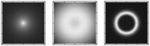
3.1.2. Numerical example for a triangular molecule

In the particle density plots, larger molecules would also be seen as ‘round’ objects in their eigenstates with zero total angular momentum and positive parity (N=0,p=+1), and localised particles form shells around the molecular centre of mass. In order to demonstrate a non-trivial arrangement of the atomic nuclei within a molecule, the H${}_2$D${}^{+}=\{{\mathrm{p}}^{+},{\mathrm{p}}^{+},{\mathrm{d}}^{+},{\mathrm{e}}^{-},{\mathrm{e}}^{-}\}$ molecular ion was studied in Ref. [73]. Interestingly, the qualitative features of the computed density functions (see Figure 6) converged very fast, small basis sets and a loose parameterisation was sufficient to observe converged structural features, whereas the energies were far from spectroscopic accuracy.

Figure 6. Radial, ${\rho }_{ab}$, and angular, ${\mathit{\Gamma }}_{\mathit{a}\mathit{,}\mathit{b}\mathit{c}}$, probability density functions computed for H${}_2$D${}^{+}=\{{\mathrm{e}}^{-},{\mathrm{e}}^{-},{\mathrm{p}}^{+},{\mathrm{p}}^{+},{\mathrm{d}}^{+}\}$.

Figure 6 summarises the particle-density functions which highlight characteristic structural features of the system. First, we can observe the delocalised electron cloud (${\rho }_{0,\mathrm{e}}$), the proton shell (${\rho }_{0,\mathrm{p}}$), and the deuteron shell (${\rho }_{0,\mathrm{d}}$) around the centre of mass (0). The deuteron shell is more peaked and more localised in comparison with the proton shell. (Remember that these plots show the spherically symmetric density along a ray, ${\rho }_{ab}$, and the density functions are normalised to one.)

Next, let's look at the probability density functions for the included angle, ${\mathit{\Gamma }}_{0,ab}$, of two particles measured from the molecular centre of mass (‘0’). The dashed line in the plots shows the angular density corresponding to a hypothetical system in which the two particles (a and b) are independent. It is interesting to note that for the two electrons ${\mathit{\Gamma }}_{0,\mathrm{e}{\mathrm{e}}^{\prime }}$ shows very small deviation from the (uncorrelated system's) dashed line. At the same time, we see a pronounced deviation from the dashed line for the nuclei, ${\mathit{\Gamma }}_{0,\mathrm{p}{\mathrm{p}}^{\prime }}$ and ${\mathit{\Gamma }}_{0,\mathrm{pd}}$. These numerical observations are in line with Claverie and Diner's suggestion based on theoretical considerations [103] that molecular structure could be seen in an fully quantum-mechanical description as correlation effects for the nuclei.

As to the included angle of the two protons and the deuteron, the ${\mathit{\Gamma }}_{\mathrm{d}\mathit{,}\mathrm{p}{\mathrm{p}}^{\prime }}$ probability density function has a maximum at around 60 degrees, which indicates the triangular arrangement of the nuclei. Due to the almost negligible amplitude of ${\mathit{\Gamma }}_{\mathrm{d}\mathit{,}\mathrm{p}{\mathrm{p}}^{\prime }}$ at around 180 degrees the linear arrangement of the three nuclei (in the ground state) can be excluded. Thus, the structure of H${}_2$D${}^{+}$ derived from our pre-BO numerical study is in agreement with the equilibrium structure (equilateral triangle) known from BO electronic-structure computations.

3.2. Classical structure from quantum mechanics

Relying on the probabilistic interpretation of quantum mechanics, the structure of H${}_2^{+}$ was visualised as a proton shell (Figure 5) with the protons found at around the antipodal points, and H${}_2$D${}^{+}$ was seen as a proton shell and a deuteron shell within which the relative position of the three nuclei is dominated by a triangular arrangement (Figure 6). This analysis has demonstrated that elements of molecular structure can be recognised in the appropriate marginal probability densities calculated from the full electron-nuclear wave function. At the same time, a chemist would rather think about H${}_2^{+}$ as a (classical) rotating dumbbell (Figure 7) and H${}_2$D${}^{+}$ as a (nearly) equilateral triangle. Although elements can be recognised in the probability density functions, the link to the classical structure which chemists have used for more than a century to understand and design new reaction pathways for new materials, is not obvious [97,99,100,102,121, 122].

Figure 7. Quantum vs. classical structure of molecules: superposition or rotating dumbbell.

In the next couple of paragraphs we briefly outline a promising direction which can offer a resolution to this puzzle. We collect the most relevant aspects and ideas, whereas their detailed exploration is left for future work in this field. In order to recover the classical molecular structure from a fully quantum mechanical treatment, it is necessary to obtain for a molecule

1. the shape;

2. the handedness: chiral molecules are found exclusively in their left- or right-handed version or in a classical mixture (called racemic mixture) of these mirror images but ‘never’ in their superposition;

3. the individual labelling of the atomic nuclei (distinguishability).

Although it is possible to write down appropriate linear combinations (wave packets) of eigenstates of the full Hamiltonian, which satisfy these requirements at certain moments, we would like to recover these properties as permanent molecular observables. (Most recently, Grohmann and Manz [123] have pointed on the fact that it is impossible to form localised superpositions of quantum states of molecular rotors, which would coincide with our (semi)classical picture of methyl groups, due to the different spin part corresponding to the spatial functions which would be necessary for these superpositions.)

A possible resolution of the quantum-classical molecular structure puzzle will start out from the description of the molecule as an open quantum system being in interaction with an environment [124,125]. According to decoherence theory pointer states are selected by the continuous monitoring of the environment. As a result, the system's reduced density matrix (after tracing out the environmental degrees of freedom from the world's density matrix) written in this pointer basis evolves in time so that its off-diagonal elements decay exponentially with some decoherence time, characteristic to the underlying microscopic interaction process with the environment (radiation or matter). This decay of the off-diagonal elements leads to the suppression of the interference terms between different pointer states, and results in a (reduced) density matrix the form of which corresponds to that of mixed states. Hence, this result can be interpreted as the emergence of the classical features in a quantum mechanical treatment.⁴ So, decoherence theory allows us to identify pointer states, which are selected and remain stable as a result of the molecule's interaction with its environment.

It is interesting to note that important molecular properties (shape, handedness, atomic labels) break the fundamental symmetries of an isolated quantum system: the rotational and inversion symmetry, as well as the indistinguishability of identical particles. It remains a task to explore on a detailed microscopic level how and why these broken-symmetry states become pointer states of a molecular system.

1. Shape. Following the pioneering studies which have identified pointer states and confirmed their stability upon translational localisation [126–128] Ref. [129] provides a detailed account of the rotational decoherence of mesoscopic objects induced by a photon-gas environment or massive particles in thermal equilibrium. The qualitative conclusions are similar for the two different environments, but there are differences in the estimated decoherence time and its temperature dependence differ for the two environments. Orientational localisation of the mesoscopic ellipsoid takes place only if there are at least two directions for which the electric polarisabilities are different, and coherence is suppressed exponentially with the angular distance between two orientations.

2. Handedness. As to the chirality of molecules, the superselection phenomenon has been demonstrated in Ref. [130] by using a master equation [131] which describes the incoherent dynamics of the molecular state in the presence of the scattering of a lighter, thermalised background gas. Experimental conditions are predicted under which the tunnelling dynamics is suppressed between the left and right-handed configurations of D${}_2$S${}_2$.

3. Individual labelling of the atomic nuclei. Concerning the distinguishability of atomic nuclei, it remains a challenge to work out the detailed theoretical equations and to estimate the experimental conditions under which the individual labelling of quantum mechanically identical atomic nuclei (e.g. protons) emerges.

4. Summary, conclusions, and future challenges

The direct solution of the full electron-nuclear Schrödinger equation, without the introduction of any kind of separation of the electronic and the nuclear motion, makes it possible to approach the non-relativistic limit arbitrarily close. We call this approach to the molecular problem pre-Born–Oppenheimer (pre-BO) theory in order to emphasise that the usual BO separation is avoided. The article presented details of our pre-BO computational method, which we call QUANTEN (QUANTum mechanical treatment of Electrons and atomic Nuclei), using explicitly correlated Gaussian functions and the stochastic variational method with relevant citations to the pioneers of these computational techniques [18,19,38].

We have reviewed numerical results obtained for several bound and a couple of unbound states of three- and four-particle systems with various quantum numbers and with sub-spectroscopic accuracy in the energy. Although these computations are very demanding, they will allow us to test the results provided by more efficient, effective Hamiltonians obtained for example from non-adiabatic perturbation theory [92]. It is also interesting to notice that rovibrational states bound by an excited electronic state within the BO approximation are obtained as resonances within a pre-BO treatment with direct access to not only the energy but also to the finite predissociation lifetime of the state (due to rovibronic couplings). Numerical results demonstrating this idea were discussed for the hydrogen molecule.

At the moment, larger (polyatomic) systems can be addressed with a much reduced accuracy (in the energy) with the various existing pre-BO methods. Indeed, it has been an open problem for many years to define efficient basis functions and/or parameterisation strategies which make a pre-BO treatment amenable for polyatomics with (sub-)spectroscopic accuracy. As soon as polyatomic pre-BO computations of (sub-)spectroscopic accuracy will become possible (even if only a few states of selected non-relativistic quantum numbers can be computed), rigorous variational benchmark values will become available to the effective non-adiabatic theories, which can be efficiently used to compute all rovibrational (rovibronic) bound and many resonance states. At the moment results of these effective non-adiabatic computations can be compared only with experimentally measured spectroscopic transitions for which relativistic (and probably also some QED) correction must be included, which would also need to be validated. Already at the present stage and possibilities of pre-BO theory, less accurate computations of polyatomic molecules shed light to a long-standing problem: the reconstruction of the chemist's (classical) molecular structure form a fully quantum mechanical description. We reviewed computational results, which allowed us to identify elements of the molecular structure from the full electron-nuclear wave function by inspecting and finding local maxima of appropriately defined marginal probability density functions.

We believe that this, currently less common, route to describe molecular systems, i.e., an equal quantum mechanical treatment of electrons and atomic nuclei, opens up great possibilities and also sets outstanding challenges for future theoretical work and for applications in comparison with the latest experimental developments. To conclude this article, we highlight three important directions to motivate further work in this old-new field of molecular quantum mechanics:

1. Fully quantum mechanical developments for precision spectroscopy of small molecules The comparison of precision measurements and highly accurate molecular computations for small and light molecules contributes to the testing of fundamental physical constants, e.g. the proton-to-electron mass ratio, the fine structure constant, or to pinpoint fundamental physical quantities, such as the proton radius, and to test fundamental physical theories [132,133]. For a meaningful comparison, it is mandatory to be able to solve the non-relativistic Schrödinger equation very accurately for several (bound and unbound) states of di- and polyatomic molecules and to account for the relativistic as well as QED effects.

2. A hierarchy of approximate pre-BO methods The idea of including the atomic nuclei in the quantum mechanical treatment of the electrons has been pursued in order to develop a systematically improvable, hierarchy of approximate pre-BO methods [23–29, 134,135]. An appealing feature of a pre-BO treatment is that it allows us to avoid the computation and fitting of the potential energy surface(s) and non-adiabatic coupling vectors (for multiple electronic states). At the moment, it appears to be technically and computationally extremely challenging to devise a practical, accurate, and systematically improvable hierarchy of approximate electron-nuclear methods applicable to larger, polyatomic molecules. Recently, a combination of electronic structure and quantum nuclear motion theory has been suggested [30,136], which aims to combine the best of the two worlds in a practical manner.

3. Chemical observables from a fully quantum mechanical treatment The definition of molecular structure within a fully quantum mechanical (pre-BO) description of molecules remains to be an unsettled problem [97,99,100,102,121,122] either for a numerically ‘exact’ or an approximate treatment. Certainly, the probabilistic interpretation of the molecular wave function and the study of appropriate marginal probability densities provide useful pieces of information about the structure of a molecule. In order to arrive at a quantum molecular theory, in which the molecule is treated quantum mechanically as a whole, and at the same time the known chemical concepts are restored from the theoretical treatment, it is necessary to re-establish the shape, the handedness, and the individual labelling of the identical atomic nuclei. Interestingly, these important chemical properties break the fundamental symmetries of an isolated quantum system. The application of decoherence theory with realistic microscopic models for molecules offers a reasonable starting point for the reconstruction of these known classical chemical properties. The estimation of decoherence time for various environments and interactions has relevance for the practical realisation of quantum control and quantum computing experiments with molecules.

Acknowledgements

The author is indebted to Professors Brian Sutcliffe, Markus Reiher, Ulrich Müller-Herold, and Jürg Hutter, as well as to Dr. Benjamin Simmen and Andrea Muolo for their interest, discussions, and joint work over the years on various aspects of this topic.

Disclosure statement

No potential conflict of interest was reported by the author.

ORCID

Edit Mátyus http://orcid.org/0000-0001-7298-1707

Additional information

Funding

Financial support from a PROMYS Grant (no. IZ11Z0_166525) of the Swiss National Science Foundation is gratefully acknowledged.

Notes

1. We use the spectroscopists' notation [137] for the total angular momentum quantum number, N, instead of L that is commonly used in the physics literature.

2. The term “spectroscopic accuracy” is not uniquely defined but it is usually used to refer to computations providing vibrational transition wave numbers with an uncertainty better than 1 cm⁻¹ ($\approx 4.6\mu$E${}_{\mathrm{h}}$) and even higher accuracy for rotational transitions.

3. For example, the IUPAC's Compendium of Chemical Terminology (‘Gold Book’) [138] defines the equilibrium geometry in terms of a potential energy surface, but we do not find anything beyond the BO approximation, apart from the definition of the primary, secondary, etc. structures of macromolecules. Interestingly, the molecular shape is defined in the Compendium.

4. There is an unsettled discussion concerning the mixed states of open quantum systems in terms of proper vs. improper mixtures, which is related to the quantum measurement problem [139,140].

References

- A.J. Rocke, in Image & Reality: Kekulé, Kopp, and the Scientific Imagination (Synthesis), A Series in the History of Chemistry (The University of Chicago Press, Chichago and London, 2010).
- E. Schrödinger, Phys. Rev. 28, 1049 (1926). doi: 10.1103/PhysRev.28.1049
- M. Born and R. Oppenheimer, Ann. der Phys. 84, 457 (1927). doi: 10.1002/andp.19273892002
- M. Born, Nachr. Akad. Wiss. Göttingen, math.-phys. Kl., math.-phys.-chem. Abtlg. 6, 1 (1951).
- M. Born and K. Huang, Dynamical Theory of Crystal Lattices (Clarendon Press, Oxford, 1954).
- B.T. Sutcliffe and R.G. Woolley, in The Potential Energy Surface in Molecular Quantum Mechanics (Springer International Publishing Switzerland, 2013), vol. 27 of Advances in Quantum Methods and Applications in Chemistry, Physics, and Biology, Progress in Theoretical Chemistry and Physics, pp. 3–40.
- B.T. Sutcliffe and R.G. Woolley, J. Chem. Phys. 137, 22A544 (2012). doi: 10.1063/1.4755287
- B.T. Sutcliffe, Coordinate Systems and Transformations, in Handbook of Molecular Physics and Quantum Chemistry, edited by S. Wilson (John Wiley & Sons, Inc., Chichester, 2003a), Vol. 1, pp. 485–500.
- B.T. Sutcliffe, Molecular Hamiltonians, in Handbook of Molecular Physics and Quantum Chemistry, edited by S. Wilson (John Wiley & Sons, Inc., Chichester, 2003b), Vol. 1, pp. 501–525.
- D. Luckhaus, J. Chem. Phys. 113, 1329 (2000). doi: 10.1063/1.481924
- D. Lauvergnat and A. Nauts, J. Chem. Phys. 116, 8560 (2002). doi: 10.1063/1.1469019
- N. Yurchenko, W. Thiel and P. Jensen, J. Mol. Spectrosc. 245, 126 (2007). doi: 10.1016/j.jms.2007.07.009
- E. Mátyus, G. Czakó and A.G. Császár, J. Chem. Phys. 130, 134112 (2009). doi: 10.1063/1.3076742
- C. Fábri, E. Mátyus and A.G. Császár, J. Chem. Phys. 134, 074105 (2011). doi: 10.1063/1.3533950
- S.N. Yurchenko, J. Tennyson, J. Bailey, M.D.J. Hollis and G. Tinettia, Proc. Nat. Acad. Sci. USA111, 9379 (2014). doi: 10.1073/pnas.1324219111
- J. Tennyson, J. Chem. Phys. 145, 120901 (2016). doi: 10.1063/1.4962907
- T. Carrington, Jr., J. Chem. Phys. 146, 120902 (2017). doi: 10.1063/1.4979117
- M. Cafiero, S. Bubin and L. Adamowicz, Phys. Chem. Chem. Phys. 5, 1491 (2003). doi: 10.1039/b211193d
- S. Bubin, M. Pavanello, W.-C. Tung, K.L. Sharkey and L. Adamowicz, Chem. Rev. 113, 36 (2013). doi: 10.1021/cr200419d
- E. Mátyus and M. Reiher, J. Chem. Phys. 137, 024104 (2012). doi: 10.1063/1.4731696
- B. Simmen, E. Mátyus and M. Reiher, J. Chem. Phys. 141, 154105 (2013a).
- A. Muolo, E. Mátyus and M. Reiher, J. Chem. Phys. 148, 084112 (2018). doi: 10.1063/1.5009465
- H. Nakai, Int. J. Quant. Chem. 86, 511 (2002). doi: 10.1002/qua.1106
- A.D. Bochevarov, E.F. Valeev and C.D. Sherrill, Mol. Phys. 102, 111 (2004). doi: 10.1080/00268970410001668525
- A. Chakraborty, M.V. Pak and S. Hammes-Schiffer, J. Chem. Phys. 129, 014101 (2008).
- T. Ishimoto, M. Tachikawa and U. Nagashima, Int. J. Quant. Chem. 109, 2677 (2009). doi: 10.1002/qua.22069
- A. Sirjoosingh, M.V. Pak, C. Swalina and S. Hammes-Schiffer, J. Chem. Phys. 139, 034102 (2013).
- N.F. Aguirre, P. Villarreal, G. Delgado-Barrio, E. Posada, A. Reyes, M. Biczysko, A.O. Mitrushchenkov and M.P. de Lara-Castells, J. Chem. Phys. 138, 184113 (2013). doi: 10.1063/1.4803546
- R. Flores-Moreno, E. Posada, F. Moncada, J. Romero, J. Charry, M. Díaz-Tinoco, S.A. González, N.F. Aguirre and A. Reyes, Int. J. Quant. Chem. 114, 50 (2013). doi: 10.1002/qua.24500
- P. Cassam-Chenaï, B. Suo and W. Liu, Phys. Rev. A 92, 012502 (2015). doi: 10.1103/PhysRevA.92.012502
- D.M. Bishop and L.M. Cheung, Chem. Phys. Lett. 79, 130 (1981). doi: 10.1016/0009-2614(81)85303-1
- V.I. Korobov, Phys. Rev. A 61, 064503 (2000). doi: 10.1103/PhysRevA.61.064503
- J.P. Karr and L. Hilico, J. Phys. B: At. Mol. Opt. Phys. 39, 2095 (2006). doi: 10.1088/0953-4075/39/8/024
- K. Pachucki, M. Zientkiewicz and V. Yerokhin, Comput. Phys. Commun. 208, 162 (2016). doi: 10.1016/j.cpc.2016.07.024
- J. Rychlewski, ed., Explicitly Correlated Wave Functions in Chemistry and Physics (Kluwer Academic Publishers, Dodrecht, 2003).
- J. Mitroy, S. Bubin, W. Horiuchi, Y. Suzuki, L. Adamowicz, W. Cencek, K. Szalewicz, J. Komasa, D. Blume and K. Varga, Rev. Mod. Phys. 85, 693 (2013). doi: 10.1103/RevModPhys.85.693
- L. K. F. A. Bischoff and E. F. Valeev, Chem. Rev. 112, 75 (2012). doi: 10.1021/cr200204r
- Y. Suzuki and K. Varga, Stochastic Variational Approach to Quantum-Mechanical Few-Body Problems (Springer-Verlag, Berlin, 1998).
- D.B. Kinghorn and R.D. Poshusta, Phys. Rev. A 47, 3671 (1993). doi: 10.1103/PhysRevA.47.3671
- P.M. Kozlowski and L. Adamowicz, Phys. Rev. A 48, 1903 (1993). doi: 10.1103/PhysRevA.48.1903
- D.B. Kinghorn and R.D. Poshusta, Int. J. Quant. Chem. 62, 223 (1997). doi: 10.1002/(SICI)1097-461X(1997)62:2<223::AID-QUA10>3.0.CO;2-C
- D.B. Kinghorn and L. Adamowicz, J. Chem. Phys. 110, 7166 (1999a). doi: 10.1063/1.478620
- D.B. Kinghorn and L. Adamowicz, Phys. Rev. Lett. 83, 2541 (1999b). doi: 10.1103/PhysRevLett.83.2541
- N. Kirnosov, K.L. Sharkey and L. Adamowicz, J. Phys. B: At. Mol. Opt. Phys. 48, 195101 (2015). doi: 10.1088/0953-4075/48/19/195101
- K. Jones, M. Formanek, R. Mazumder, N. Kirnosov and L. Adamowicz, Mol. Phys. 114, 1634 (2016a). doi: 10.1080/00268976.2016.1142621
- K. Jones, N. Kirnosov, K.L. Sharkey and L. Adamowicz, Mol. Phys. 114, 2052 (2016b). doi: 10.1080/00268976.2016.1177666
- K. Jones, M. Formanek and L. Adamowicz, Chem. Phys. Lett. 669, 188 (2017). doi: 10.1016/j.cplett.2016.12.049
- E. Bednarz, S. Bubin and L. Adamowicz, Mol. Phys. 103, 1169 (2005). doi: 10.1080/00268970512331339314
- S. Bubin and L. Adamowicz, J. Chem. Phys. 124, 224317 (2006). doi: 10.1063/1.2204605
- S. Bubin and L. Adamowicz, J. Chem. Phys. 128, 114107 (2008). doi: 10.1063/1.2894866
- D. Kedziera, M. Stanke, S. Bubin, M. Barysz and L. Adamowicz, J. Chem. Phys. 125, 084303 (2006).
- M. Stanke, S. Bubin, M. Molski and L. Adamowicz, Phys. Rev. A 79, 032507 (2009).
- S. Bubin, M. Stanke, M. Molski and L. Adamowicz, Chem. Phys. Lett. 494, 21 (2010a). doi: 10.1016/j.cplett.2010.05.081
- S. Bubin, M. Stanke and L. Adamowicz, Chem. Phys. Lett. 500, 229 (2010b). doi: 10.1016/j.cplett.2010.10.021
- S. Bubin, M. Stanke and L. Adamowicz, J. Chem. Phys. 134, 024103 (2011a). doi: 10.1063/1.3525679
- S. Bubin, M. Stanke and L. Adamowicz, Phys. Rev. A 83, 042520 (2011b).
- S. Bubin, M. Stanke and L. Adamowicz, J. Chem. Phys. 135, 074110 (2011c).
- S. Bubin, M. Stanke and L. Adamowicz, J. Chem. Phys. 131, 044128 (2009).
- K. Varga and Y. Suzuki, Phys. Rev. C 52, 2885 (1995). doi: 10.1103/PhysRevC.52.2885
- Y. Suzuki, J. Usukura and K. Varga, J. Phys. B: At. Mol. Opt. Phys. 31, 31 (1998). doi: 10.1088/0953-4075/31/1/007
- T. Joyce and K. Varga, J. Chem. Phys. 144, 184106 (2016). doi: 10.1063/1.4948708
- J. Usukura, K. Varga and Y. Suzuki, Phys. Rev. A 58, 1918 (1998). doi: 10.1103/PhysRevA.58.1918
- G. Ryzhikh, J. Mitroy and K. Varga, J. Phys. B: At. Mol. Opt. Phys. 31, 3965 (1998). doi: 10.1088/0953-4075/31/17/019
- K. Varga, J. Usukura and Y. Suzuki, Phys. Rev. Lett. 80, 1876 (1998). doi: 10.1103/PhysRevLett.80.1876
- J. Usukura, Y. Suzuki and K. Varga, Phys. Rev. B 59, 5652 (1999). doi: 10.1103/PhysRevB.59.5652
- Y. Suzuki and J. Usukura, Nucl. Instrum. Methods Phys. Res. B 171, 67 (2000). doi: 10.1016/S0168-583X(00)00055-0
- I.A. Ivanov, J. Mitroy and K. Varga, Phys. Rev. Lett. 87, 063201 (2001).
- J.Z. Mezei, J. Mitroy, R.G. Lovas and K. Varga, Phys. Rev. A 64, 032501 (2001). doi: 10.1103/PhysRevA.64.032501
- E.A.G. Armour, J.-M. Richard and K. Varga, Phys. Rep. 413, 1 (2005). doi: 10.1016/j.physrep.2005.02.003
- E. Mátyus, J. Phys. Chem. A 117, 7195 (2013). doi: 10.1021/jp4010696
- B. Simmen, E. Mátyus and M. Reiher, Mol. Phys. 111, 2086 (2013b). doi: 10.1080/00268976.2013.783938
- E. Mátyus, J. Hutter, U. Müller-Herold and M. Reiher, Phys. Rev. A 83, 052512 (2011a). doi: 10.1103/PhysRevA.83.052512
- E. Mátyus, J. Hutter, U. Müller-Herold and M. Reiher, J. Chem. Phys. 135, 204302 (2011b). doi: 10.1063/1.3662487
- Y. Suzuki, W. Horiuchi, M. Orabi and K. Arai, Few-Body Syst. 42, 33 (2008). doi: 10.1007/s00601-008-0200-3
- I. Mayer, Simple Theorems, Proofs, and Derivations in Quantum Chemistry (Kluwer Academic/Plenum Publishers, New York, 2003).
- M.J.D. Powell, The NEWUOA Software for Unconstrained Optimization without Derivatives (DAMTP 2004/NA05), Report no. NA2004/08. <http://www.damtp.cam.ac.uk/user/na/reports04.html> last acces-sed on January 18, 2013.
- J. Usukura and Y. Suzuki, Phys. Rev. A 66, 010502(R) (2002). doi: 10.1103/PhysRevA.66.010502
- Y. Suzuki and J. Usukura, Nucl. Instrum. Methods Phys. Res. B 221, 195 (2004). doi: 10.1016/j.nimb.2004.03.054
- A.U. Hazi and H.S. Taylor, Phys. Rev. A 1, 1109 (1970). doi: 10.1103/PhysRevA.1.1109
- H.S. Taylor and A.U. Hazi, Phys. Rev. A 14, 2071 (1976). doi: 10.1103/PhysRevA.14.2071
- V.A. Mandelshtam, H.S. Taylor, V. Ryaboy and N. Moiseyev, Phys. Rev. A 50, 2764 (1994). doi: 10.1103/PhysRevA.50.2764
- J. Müller, X. Yang and J. Burgdörfer, Phys. Rev. A 49, 2470 (1994). doi: 10.1103/PhysRevA.49.2470
- V.I. Kukulin, V.M. Krasnopolsky and J. Horácek, Theory of Resonances—Principles and Applications (Kluwer, Dodrecth, 1988).
- E. Anderson, Z. Bai, C. Bischof, S. Blackford, J. Demmel, J. Dongarra, J. Du Croz, A. Greenbaum, S. Hammarling and A. McKenney, et al., LAPACK Users' Guide, 3rd ed. (Society for Industrial and Applied Mathematics, Philadelphia, PA, 1999), ISBN 0-89871-447-8 (paperback).
- K. Piszczatowski, G. Lach, M. Przybytek, J. Komasa, K. Pachucki and B. Jeziorski, J. Chem. Theo. Comp. 5, 3039 (2009). doi: 10.1021/ct900391p
- B. Simmen, E. Mátyus and M. Reiher, J. Phys. B 48, 245004 (2015). doi: 10.1088/0953-4075/48/24/245004
- B. Simmen, Developments for a Relativistic Many-1/2-Fermion Theory, PhD thesis ETH Zürich, Nr. 22363 (2015). <http://dx.doi.org/10.3929/ethz-a-010398188>.
- M. Stanke and L. Adamowicz, J. Phys. Chem. A 117, 10129 (2013). doi: 10.1021/jp4020492
- M. Stanke, J. Jurkowski and L. Adamowicz, J. Phys. B 50, 065101 (2017). doi: 10.1088/1361-6455/aa56ad
- V.I. Korobov, L. Hilico and J. Karr, Phys. Rev. A 74, 040502(R) (2006). doi: 10.1103/PhysRevA.74.040502
- S. Bubin and L. Adamowicz, J. Chem. Phys. 118, 3079 (2003). doi: 10.1063/1.1537719
- K. Pachucki and J. Komasa, J. Chem. Phys. 130, 164113 (2009). doi: 10.1063/1.3114680
- L. Wolniewicz, T. Orlikowski and G. Staszewska, J. Mol. Spectrosc. 238, 118 (2006). doi: 10.1016/j.jms.2006.04.020
- L. Wolniewicz, Mol. Phys. 105, 1497 (2007). doi: 10.1080/00268970701257082
- W. Kołos and J. Rychlewski, J. Mol. Spectrosc. 143, 237 (1990). doi: 10.1016/0022-2852(91)90088-R
- W. Kołos and J. Rychlewski, J. Mol. Spectrosc. 66, 428 (1977). doi: 10.1016/0022-2852(77)90301-0
- H. Primas, Chemistry, Quantum Mechanics and Reductionism: Perspectives in Theoretical Chemistry (Springer-Verlag, Berlin, 1981).
- M. Cafiero and L. Adamowicz, Chem. Phys. Lett. 387, 136 (2004). doi: 10.1016/j.cplett.2004.02.006
- B.T. Sutcliffe and R.G. Woolley, Phys. Chem. Chem. Phys. 7, 3664 (2005). doi: 10.1039/b509723c
- B.T. Sutcliffe and R.G. Woolley, Chem. Phys. Lett. 408, 445 (2005). doi: 10.1016/j.cplett.2005.04.022
- S.J. Weininger, J. Chem. Educ. 61, 939 (1984). doi: 10.1021/ed061p939
- R.G. Woolley, Adv. Phys. 25, 27 (1976). doi: 10.1080/00018737600101352
- P. Claverie and S. Diner, Isr. J. Chem. 19, 54 (1980). doi: 10.1002/ijch.198000006
- J.G.R. Tostes, Theor. Chim. Acta 59, 229 (1981). doi: 10.1007/BF00551352
- U. Müller-Herold, J. Chem. Phys. 124, 014105 (2006). doi: 10.1063/1.2141509
- U. Müller-Herold, Eur. Phys. J. D 49, 311 (2008). doi: 10.1140/epjd/e2008-00174-3
- E.V. Ludeña, L. Echevarría, X. Lopez and J.M. Ugalde, J. Chem. Phys. 136, 084103 (2012). doi: 10.1063/1.3682244
- M. Becerra, V. Posligua, and E.V. Ludeña, Int. J. Quant. Chem. 113, 1584 (2013). doi: 10.1002/qua.24368
- M. Goli and S. Shahbazian, Theor. Chim. Acta 129, 235 (2011). doi: 10.1007/s00214-011-0927-7
- M. Goli and S. Shahbazian, Theor. Chim. Acta 131, 1208 (2012). doi: 10.1007/s00214-012-1208-9
- T. Kato and K. Yamanouchi, Phys. Rev. A 85, 034504 (2012). doi: 10.1103/PhysRevA.85.034504
- J.F. Pérez-Torres, Phys. Rev. A 87, 062512 (2013). doi: 10.1103/PhysRevA.87.062512
- J.F. Pérez-Torres, J. Phys. Chem. A 119, 2895 (2015). doi: 10.1021/acs.jpca.5b00907
- V. Pohl and J.C. Tremblay, Phys. Rev. A 93, 012504 (2016). doi: 10.1103/PhysRevA.93.012504
- A. Martin, J.-M. Richard and T.T. Wu, Phys. Rev. A 46, 3697 (1992). doi: 10.1103/PhysRevA.46.3697
- A.A. Farajian, K. Esfarjani and Y. Kawazoe, J. Phys. B 32, 749 (1999). doi: 10.1088/0953-4075/32/3/016
- A. Fröman and J.L. Kinsey, Phys. Rev. 123, 2077 (1961). doi: 10.1103/PhysRev.123.2077
- F.L. Andrew, W. King and H. Cox, J. Chem. Phys. 139, 224306 (2013).
- A.W. King, L.C. Rhodes and H. Cox, Phys. Rev. A 93, 022509 (2016).
- A.L. Baskerville, A.W. King and H. Cox, Phys. Rev. A 94, 042512 (2016). doi: 10.1103/PhysRevA.94.042512
- F. Hund, Z. Phys. 43, 805 (1927). doi: 10.1007/BF01397249
- P. Cassam-Chenaï, Chem. Phys. Lett. 420, 354 (2006). doi: 10.1016/j.cplett.2006.01.004
- T. Grohmann and J. Manz, Mol. Phys. 116, 2538 (2018). doi: 10.1080/00268976.2018.1473651
- E. Joos, H. Zeh, C. Kiefer, D. Giulini, J. Kupsch, and I. Stamatescu, Decoherence and the Appearance of a Classical World in Quantum Theory, 2nd ed. (Springer-Verlag, Berlin Heidelberg New York, 2003).
- M. Schlosshauer, Decoherence and the Quantum-to-Classical Transition (Springer, Berlin, 2007).
- K. Hornberger and J.E. Sipe, Phys. Rev. A 68, 012105 (2003). doi: 10.1103/PhysRevA.68.012105
- S.L. Adler, J. Phys. A: Math. Theor. 39, 14067 (2006). doi: 10.1088/0305-4470/39/45/015
- M. Busse and K. Hornberger, J. Phys. A: Math. Theor. 43, 015303 (2009).
- C. Zhong and F. Robicheaux, Phys. Rev. A 94, 052109 (2016). doi: 10.1103/PhysRevA.94.052109
- J. Trost and K. Hornberger, Phys. Rev. Lett. 103, 023202 (2009). doi: 10.1103/PhysRevLett.103.023202
- K. Hornberger, Eur. Phys. Lett. 77, 50007 (2007). doi: 10.1209/0295-5075/77/50007
- J.-P. Karr, S. Patra, J. Koelemeij, J. Heinrich, N. Sillitoe, A. Douillet and L. Hilico, J. Phys.: Conf. Ser. 723, 012048 (2016).
- W. Ubachs, J. Koelemeij, K. Eikema and E. Salumbides, J. Mol. Spectrosc. 320, 1 (2016). doi: 10.1016/j.jms.2015.12.003
- T. Ishimoto, M. Tachikawa and U. Nagashima, J. Chem. Phys. 128, 164118 (2008).
- A. Sirjoosingh, M.V. Pak, K.R. Brorsen and S. Hammes-Schiffer, J. Chem. Phys. 142, 214107 (2015). doi: 10.1063/1.4921303
- P. Cassam-Chenaï, B. Suo and W. Liu, Theor. Chim. Acta 136, 52 (2017). doi: 10.1007/s00214-017-2081-3
- E. Cohen, T. Cvitaš, J. Frey, B. Holmström, K. Kuchitsu, R. Marquardt, I. Mills, F. Pavese, M. Quack, J. Stohner, H. Strauss, M. Takami and A.J. Thor, Quantities, Units and Symbols in Physical Chemistry (the IUPAC Green Book - 3rd edition) (RSC Publishing, Cambridge, 2007).
- IUPAC Compendium of Chemical Terminology—the Gold Book. <https://goldbook.iupac.org/> last acces-sed on February 28, 2018..
- S. Fortin, O. Lombardi and J.C.M. González, Found. Chem. 18, 225 (2016). doi: 10.1007/s10698-016-9251-6
- G. Bacciagaluppi, The Role of Decoherence in Quantum Mechanics, The Stanford Encyclopedia of Philosophy (Fall 2016 Edition), Edward N. Zalta (ed.). <https://plato.stanford.edu/archives/fall2016/entries/qm-decoherence/> last accessed on February 28, 2018.