Full article: 2018 Table of static dipole polarizabilities of the neutral elements in the periodic table*

Formulae display: $MathJax Logo$ ?Mathematical formulae have been encoded as MathML and are displayed in this HTML version using MathJax in order to improve their display. Uncheck the box to turn MathJax off. This feature requires Javascript. Click on a formula to zoom.

ABSTRACT

A 2018 update of the most accurate calculated and experimental static dipole polarizabilities of the neutral atoms in the Periodic Table from nuclear charge Z = 1 to 120 is given. Periodic trends are analyzed and discussed.

GRAPHICAL ABSTRACT

KEYWORDS:

View correction statement:

Correction

1. Introduction

The electric dipole polarizability of an atom or molecule describes the linear response of an electronic charge distribution with respect to an externally applied electric field [Citation1,Citation2]. Atomic and molecular polarizabilities are important ingredients in many applications ranging from optical phenomena (e.g. dielectric constants, refractive indexes) to blackbody radiation shifts, atoms in optical lattices, quantum information, interatomic interactions, polarisable force-field calculations, and atomic scattering to name but a few [Citation2,Citation3]. The knowledge of accurate dipole polarizability values is therefore of utmost importance to atomic and molecular physics [Citation4]. However, despite its relevance in many fields, accurate values for atomic dipole polarizabilities are not so readily available for most elements in the periodic table, especially for open-shell systems [Citation5].

In a static homogeneous electric field, the (real and symmetric) dipole polarizability tensor of the ground electronic state is described by the quadratic Stark effect [Citation6] (in atomic units) (1) $\begin{aligned} α_{α β} & = - {\frac{\partial^{2} E}{\partial F_{α} \partial F_{β}}|}_{\vec{F} = 0} = - Re ⟨ ⟨ r_{α}; r_{β} ⟩ ⟩_{ω = 0} \\ = 2 \sum_{n} \frac{⟨ 0 | r_{α} | n ⟩ ⟨ n | r_{β} | 0 ⟩}{E_{n} - E_{0}} \end{aligned}$ (1) Where, in the perturbation expression for a multi-electron system, $r_{α}$ for the corresponding N-electron system is defined as $r_{α} = \sum_{i} r_{α, i}$ , and n runs over all electronic states (including in principle the continuum). As the quadratic Stark shift is always negative for the ground state, the dipole polarizability is always positive and non-zero. Similar expressions to (1) are obtained for the dynamic polarizability in an oscillating field of frequency ω, important in many applications such as laser physics and materials science [Citation5].

For a closed-shell atom, the polarizability for the ground state becomes scalar (tr(α)/3). However, in the most general open-shell case one needs to consider the correct Stark splitting of a specific electronic state into different |M_L| components (within the LS coupling scheme), or in the case of strong spin-orbit coupling into different |M_J| components (within the jj coupling scheme). It is clear that obtaining accurate polarizabilities for individual Stark-split states in open-shell atoms (or molecules) is very challenging for both experiment and theory [Citation7]. For open-shell cases, it is often convenient to transform to a spherical basis and express the static polarizability in terms of a scalar and tensor component (field applied in z-direction without loss of generality), i.e. in LS or jj coupling one obtains (L > 0, J > ½) (2) $\begin{aligned} α_{L}^{(L S)} (M_{L}) & = {\bar{α}}_{}^{(L S)} + α_{a}^{(L S)} \frac{3 M_{L}^{2} - L (L + 1)}{L (2 L - 1)} or \\ α_{J}^{(j j)} (M_{J}) & = {\bar{α}}_{}^{(j j)} + α_{a}^{(j j)} \frac{3 M_{J}^{2} - J (J + 1)}{J (2 J - 1)} \end{aligned}$ (2) Here $\bar{α}$ is the scalar (or average) polarizability and α_a is the (spherical) anisotropy component (tensor component). For very weak electric fields one has to consider the hyperfine splitting as well.

In the intermediate coupling regime or with several states becoming close in energy, as for open-shell lanthanide and actinide atoms, the states become multi-reference in nature and these formulae are only approximate (they only contain two independent parameters), that is each Stark-split state has to be considered separately. It becomes now clear that for many open-shell atoms the scalar polarizability and its anisotropy component are in general not strictly defined, and the values quoted depend on the underlying approximation used and electronic states considered. In other words, there is no unique definition for the scalar polarizability which we list in this paper (except for those states where the two components $\bar{α}$ and α_a are sufficient). For more details see Bonin and Kresin [Citation2].

The determination of accurate atomic polarizabilities requires a high-level electron correlation treatment within a relativistic framework, especially for the heavier elements. The gold standard in quantum chemistry is coupled cluster theory with single and double substitutions including perturbative triples, CCSD(T) [Citation8], starting from a scalar relativistic framework (e.g. Douglas-Kroll Hamiltonian (DK) [Citation9,Citation10]) or within a Dirac-Coulomb (DC) formalism including Breit interactions [Citation11]. However, for open-shell systems coupled-cluster theory is not yet so well developed at the fully relativistic level [Citation12], and one relies on multi-reference configuration interaction (MRCI) [Citation13] or many-body perturbation theory such as in complete active space methods like CASPT2 [Citation14] including spin-orbit coupling and scalar relativistic effects [Citation15]. Deviations from the exact value come from basis set incompleteness, restriction in the active orbital space chosen in the electron correlation treatment, neglect of higher-order excitations in the CI or CC treatment, incomplete treatment of Breit interactions, and the neglect of quantum electrodynamic effects, the latter being particularily important for heavy s-shell elements. For s-shell elements where the core is well separated from the valence space, one can use perturbation theory (sum-over states as shown in eq. (1) (with available experimental data as additional input) [Citation5]. Different density functionals widely used by the chemistry and physics community can lead to rather large errors in dipole polarizabilities due to the incorrect long-range and self-interaction description or the model applied [Citation16]. In such a case it is often not easy to estimate the error in published polarizability values and to make safe recommendations.

Over the past 50 years there have been a number of reviews and tabulations of atomic static dipole polarizabilities [Citation17–19], the most widely used one is that by Miller and Bederson [Citation20,Citation21]. Here we update the list of available theoretical and experimental static polarizabilites of the neutral elements up to nuclear charge 120, and try to estimate the error in the polarizability value we recommend, and briefly discuss periodic trends.

2. Experimental and calculated scalar static polarizabilities

Table lists experimental and calculated static dipole polarizabilities for all neutral atoms with nuclear charge Z = 1–120, except for livermorium where we could not find a reliable value. Not all published dipole polarizabilities are listed, only the most accurate ones we could find (e.g. experimental or theoretical from relativistic configuration interaction or coupled cluster theory). Note that there is some confusion about the experimental data listed in the CRC Handbook of Chemistry and Physics taken from Miller and Bederson [Citation57]. Some of the data are not experimental values as indicated, but from LDA calculations of Doolen, which are listed here as well. Concerning older literature, in 1971 the polarizabilities were listed up to the element radon by Teachout and Pack giving 138 references [Citation18]. A more recent review by Mitroy, Safronova and Clark is highly recommended [Citation3,Citation5]. The present list started in 2006 and the first version was published in Ref. [Citation19].

Table 1. Static scalar dipole polarizabilities (in atomic units) for neutral atoms.

Download CSV Display Table

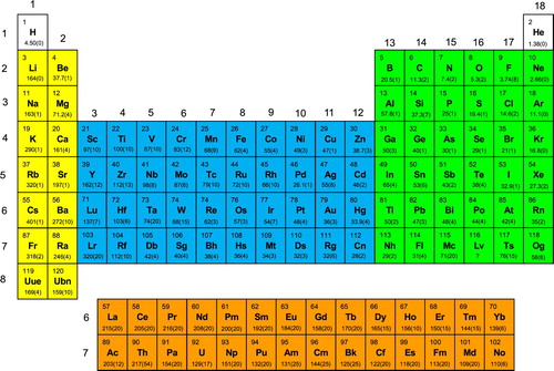
Our recommended value for each element, together with an estimate of its uncertainty, is the last value listed (in bold). Many of our estimated uncertainties are large, particularly for the heavier elements, and reflect the limited experimental and calculated results available for these elements. Obviously we had to exercise judgment in estimating the uncertainties in the recommended polarizability values. We considered both the uncertainties in polarizability values provided by the authors of the publications cited as well as the range of polarizability values available for each element. For convenience, our recommended values and accompanying uncertainties also are provided in periodic table format in Figure .

Figure 1. Recommended values from Table for the atomic polarizabilities (atomic units; estimated uncertainties in parentheses) of elements Z = 1–120. The various blocks of elements are colour-coded: s-block, yellow; p-block, green; d-block, blue; f-block, orange.

Figure 1. Recommended values from Table 1 for the atomic polarizabilities (atomic units; estimated uncertainties in parentheses) of elements Z = 1–120. The various blocks of elements are colour-coded: s-block, yellow; p-block, green; d-block, blue; f-block, orange.

The hydrogen atom deserves some special attention as its electronic spectrum is important in testing fundamental physics [Citation225]. The polarizabilities can be calculated very accurately within a relativistic framework, see Table . These calculations assume infinite nuclear mass M neglecting reduced mass corrections, finite extension of the nucleus, nuclear recoil effects (for the theory of such effects see Ref. [Citation226]), as well as quantum electrodynamic effects (QED). The reduced mass correction $f_{M}$ to the energy E_i of a specific state $| i ⟩$ can easily be evaluated by coordinate scaling $r \to r \sqrt{f_{M}}$ with $f_{M} = M / (M + m_{e})$ (m_e is the electron mass), introduced originally by Hylleraas for the nuclear charge Z [Citation227]. This leads to the original (infinite nuclear mass) Schrödinger equation, but with a ‘mass corrected’ nuclear charge $Z_{M} \to Z \sqrt{M / (M + m_{e})}$ . One can now easily verify that $E_{i} = f_{M} E_{i}^{M \to \infty}$ [Citation228]. For the ¹H and ²H hydrogen isotopes we obtain $f_{M} = 0.999456 \approx 1 - m_{e} / m_{p}$ (m_p is the proton mass) and 0.999728, respectively. The Z-dependence of the hydrogen ground state static polarizability is well known (in atomic units, α_FS is the fine structure constant), (3) $α (Z) = Z^{- 4} [\frac{9}{2} + \sum_{i} λ_{i} {(Z α_{FS})}^{2 i}]$ (3) with the expansion coefficients λ_i given by Drake and Goldman [Citation22]. Using Z_M instead and taking care of the scaling of the field term we get the mass correction for the ¹H isotope polarizability of $Δ α_{M} = + 0.00735613 a .u$ . . This increase in polarizability is easily explained as it originates mostly from the decrease in the mass corrected nuclear charge. This effect is an order of magnitude larger than the relativistic contribution. We can also estimate QED effects, as the dominant correction comes from the 1s Lamb-level shift taken from Weitz et al. [Citation229], (4) $Δ α^{QED} \approx - α [\frac{Δ E_{1 s}^{QED}}{E_{1 s}}] \approx - 1 \times 10^{- 5} a .u .$ (4) which we use for our error estimate of the final value given in Table . We note that there are only a few experiments on atomic hydrogen [Citation20], and the only directly measured value available for the hydrogen static dipole polarizability is that measured by Scheffers and Stark (α = 4.0 ± 1.3 a.u.) [Citation230,Citation231]. A dynamic dipole polarizability of 4.59 ± 0.07 a.u. and a ratio of H to H₂ polarizabilities of 0.8283 ± 0.0090, both at 587 nm [Citation232], can be combined with the experimental static dipole polarizability for H₂ of 5.437 a.u. [Citation233] to yield a value of 4.503 ± 0.049 a.u. for atomic hydrogen. This value for the static dipole polarizability of atomic hydrogen assumes that the ratio of static dipole polarizabilities is equal to the ratio of dynamic dipole polarizabilities at 587 nm. Clearly, a more accurate and directly measured experimental value for the static dipole polarizability of the hydrogen atom is needed.

3. Periodic trends

3.1. Horizontal trends

Some general periodic trends are apparent from a consideration of the polarizabilities listed in Figure . In very nearly all cases, polarizabilities decrease with increase in atomic number for each nl group of elements (e.g., the 2p elements B-Ne). This reflects the well-known decrease in size with increasing atomic number for elements in a given row of the periodic table, an effect generally attributed to increasing effective nuclear charge. Polarizabilities have units of volume, and the proportionality between atomic polarizability and volume is well known [Citation234,Citation235]. In fact, polarizabilities provide a nearly unique direct measure of the size of an isolated atom [Citation236].

In order to more clearly illustrate these periodic trends in polarizabilities, plots of polarizabilities (α; error bars reflect estimated uncertainties) versus atomic number (Z) for each of the nl-rows of elements are shown in Figures and . Empirical, weighted, nonlinear least-squares fits according to a power dependence of α on Z are included for each nl graph except for the 6d (Figure (d)) and 7p (Figure (f)) elements, for which only limited and often uncertain calculated polarizability values are available.

Figure 2. Plot of atomic polarizabilities as a function of atomic number for the p-block elements, together with weighted, nonlinear least-squares fits for all but the 7p elements (Figure (f)) according to empirical power relationships between α and Z. The ordering α(Nh, Fl) < α(Mc, Ts, Og) among the 7p elements is unusual, reflecting large relativistic effects for these atoms.

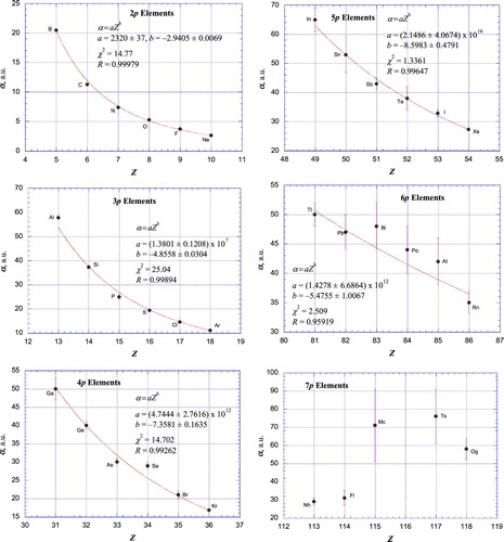
Figure 3. Plot of atomic polarizabilities as a function of atomic number for the d-block and f-block elements together with weighted, nonlinear least-squares fits according to empirical power relationships between α and Z. Pd, having the closed-shell 4d¹⁰5s⁰ electron configuration, was not included in the fit for the 4d elements (Figure (b)). Inset for 6d elements (Figure (d)): expanded view omitting Lr, having an exceptionally large polarizability due to its unique 6d⁰7s²7p_1/2¹ electron configuration, and Rf, also having a very large polarizability. A weighted, nonlinear least-squares fit of the remaining ten 6d-elements according to an empirical power relationship between α and Z is shown.

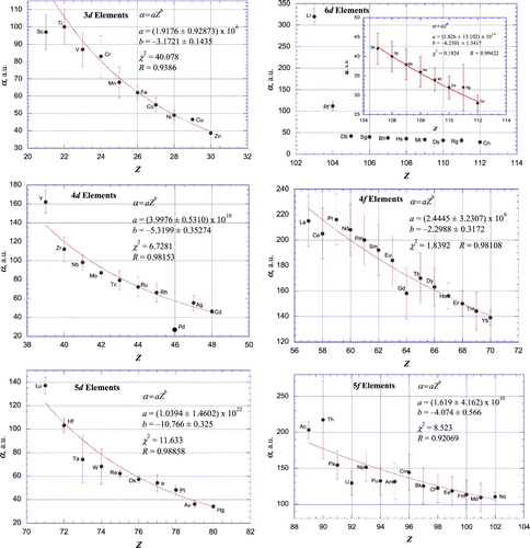
It is remarkable that for ten of the twelve nl groups of elements shown, the exceptions being the 6d (Figure (d)) and 7p (Figure (f)) elements, the polarizabilities show a power-function dependence on atomic number in which the calculated best-fit line passes through, or very close to, the error bar for nearly all of the elements included in the data fits. Pd is an exception to this observation. This discrepancy is accounted for since, among the d-block elements, the ground state of Pd (4d¹⁰5s⁰) is unique in having no electrons in a valence s orbital. The situation for Lr (6d⁰7s²7p_1/2¹) also is unique in that Lr is the only d-block element not having at least one electron in a valence d orbital [Citation237]. Other exceptions include the other Group 3 elements Sc, Y, and Lu, as well as Ac (which, together with Th, are the only f-block elements not having at least one electron in a valence f-orbital) and U. As additional, more accurate polarizabilities become available it will be interesting to see if the current, irregular variation of polarizability of the 6d and 7p elements (and, to a lesser extent, the 6p (Figure (e)) and 5f (Figure (f)) elements) with atomic number is maintained. If so, it is most likely that especially large relativistic effects on the properties of these heavy elements are responsible for their departure from the more systematic behaviour exhibited by the lighter elements.

3.2. Vertical trends

We turn now to a consideration of vertical (group) periodic trends in polarizabilities. For the Group 1 (Figure (a)) and Group 2 (Figure (b)) elements (s-block elements), polarizabilities increase with increasing period number n for the first six rows of the periodic table. The only exception to this behaviour is the slight decrease in polarizability of Na compared to Li, accounted for by the increased effective nuclear charge of Na due to its filled 2p⁶ subshell. For the last two rows, the polarizabilities decrease, a result of the large direct relativistic contraction and stabilisation of the 7s and 8s orbitals.

For the first two columns of the p-block elements, Groups 13 (Figure (a)) and 14 (Figure (b)), polarizabilities increase with increasing period number n for the first five rows, the only exception being the decrease in polarizability of Ga compared to Al, presumably reflecting the increased effective nuclear charge of Ga resulting from its filled 3d¹⁰ subshell, an effect mirrored in the relative ionisation energies of these two elements. For the last two rows of these two groups, there is a decrease in polarizabilities for Tl and Nh and for Pb and Fl compared to their lighter congeners, presumably due to the direct relativistic contraction and stabilisation of the 6p_1/2 and 7p_1/2 orbitals of these elements. For the remaining p-block elements, those of Groups 15–18 (Figure (c–f)), polarizabilities increase with increasing period number n, with no exceptions (except possibly Lv, for which no reliable polarizability value is available).

For the d-block elements, Groups 3–12, α(4d) > α(3d) except for Group 10, where α(Pd) < α(Ni), a reflection of the unique 4d¹⁰5s⁰ ground state electron configuration of Pd. For this same reason Pd is the only exception to the trend α(5d) < α(4d), while Lr and (possibly) Rf are the only exceptions to the trend α(6d) < α(5d). As noted above, the extremely large polarizability of Lr is likely a result of its unique 6d⁰7s²7p_1/2¹ ground state electron configuration.

For the f-block elements, α(4f) > α(5f) in all cases except Th, likely due to its 6d²7s² ground state electron configuration compared to 4f¹5d¹6s² for Ce, the only pair of elements among the fourteen pairs having such different ground state electron configurations.

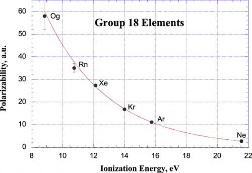
Many attempts have been made to correlate trends in atomic polarizabilities with atomic ionisation energies for a given group or column of elements in the periodic table [Citation82,Citation238]. We include graphical representations of the relationship between polarizabilities and ionisation energies [Citation239] for IUPAC Groups 1–18 (all but the f-block elements, for which there are only two members in each group or column) of the periodic table in Figures –.

Figure 4. Plot of atomic polarizabilities as a function of ionisation energy for the elements of Groups 1–6. For the Group 1 (Figure (a)) and Group 2 (Figure (b)) elements, weighted, nonlinear least-squares fits according to empirical power relationships between α and IE are included.

Figure 4. Plot of atomic polarizabilities as a function of ionisation energy for the elements of Groups 1–6. For the Group 1 (Figure 4(a)) and Group 2 (Figure 4(b)) elements, weighted, nonlinear least-squares fits according to empirical power relationships between α and IE are included.

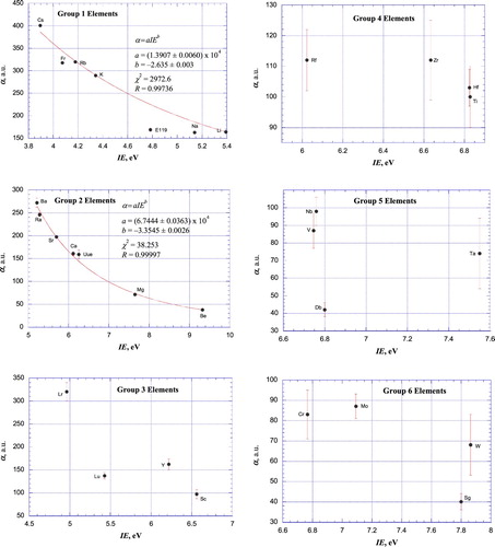
Figure 5. Plots of atomic polarizabilities as a function of ionisation energy for the elements of IUPAC Groups 7–12 together with weighted, nonlinear least-squares fits according to empirical power relationships between α and IE. Pd was not included in the data fit for the Group 10 elements (Figure (d)) due to its unique 4d¹⁰5s⁰ valence electron configuration.

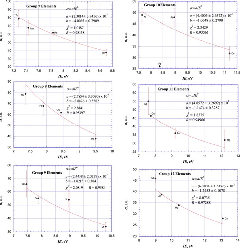
Figure 6. Plot of atomic polarizabilities as a function of ionisation energy for the elements of IUPAC Groups 13–18 together with weighted, nonlinear least-squares fit according to empirical power relationships between α and IE (Groups 13–14; Figure (a and b))) and empirical exponential relationships between α and IE (Groups 15–18; Figure (c–f))). Lv is not included among the Group 16 (Figure (a)) elements since its polarizability is not known.

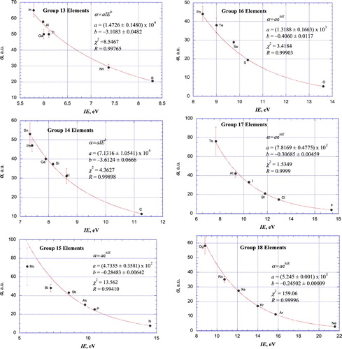
To summarise the vertical periodic trends in polarizability, it appears that useful quantitative correlations exist between polarizability and ionisation energy for Group 2 (Figure (b)) and Groups 13–18 (Figure ), although there are several outliers within these correlations, including Uue, Pt, Ir, Cd, Ga, Tl, Se, Pb, Bi, and Mc. There is too much scatter and uncertainty in the polarizabilities of Group 1 (Figure (a)) and Groups 3–12 (Figures (a,c-f) and ) to draw any firm conclusions about trends within these groups. The lack of a good correlation between the accurately known polarizabilities and ionisation energies of the Group 1 elements (Figure (a)) serves as a particularly important caveat for attempts to predict accurate polarizability values from their correlation with ionisation energies. Furthermore, for many of the heaviest elements (Z > 103), the uncertainties in the ionisation energies are as large as or greater than the errors in the polarizabilities [Citation138].

4. Conclusion

The updated list of recommended static atomic dipole polarizabilities listed in Figure and Table reveals both horizontal and vertical trends among subsets of elements. Specifically, for individual nl series of elements the polarizability decreases in a nearly smooth way with increasing atomic number. The most notable exceptions to this trend include many of the 6d (Figure (d)) and 7p (Figure (f)) elements, as well as a few other elements such as the Group 3 (Figure (a–d)) elements Sc, Y, Lu, and Lr, as well as Pd (Figure (d)) and the 5f (Figure (f)) elements Ac, Th, and U. It is unclear at this time whether such irregular dependences of polarizability on atomic number are due to large uncertainties in the limited calculated values available, or whether the particularly large relativistic effects characteristic of such heavy elements causes them to depart from the more regular periodic behaviour observed for lighter elements.

A consideration of the vertical trends among polarizabilities for the eighteen IUPAC groups of the periodic table reveals more complicated patterns where, in many cases, an increase in polarizability with increasing period number n for the lighter elements is often followed by a reversal in behaviour as the polarizabilities decrease for the heavier elements in these groups. Although there are perhaps some useful correlations between atomic polarizabilities and ionisation energies, quantitatively useful relationships appear to exist only for the Group 2 (Figure (b)) and Group 13–18 (Figure ) elements.

Experimental measurements for roughly half of the known elements are currently available, but the reliablility of many of those values is questionable. Although calculated polarizabilities are available in nearly all cases for Z = 1–120 (Lv being the only exception), there is certainly room for improvement, especially for open-shell elements and for heavy atoms that experience large relativistic effects. We hope that this review and brief analysis of polarizabilities and their periodic trends will help those interested in making experimental and computational contributions to establishing more reliable atomic polarizabilities do so. Clearly, future theoretical treatments should be done at the relativistic level using the Dirac Hamiltonian including Breit and QED effects together with an accurate treatment of electron correlation, which still is a major challenge for electronic structure theory.

An updated table of static dipole polarizabilities also is available as a pdf file from the CTCP website at Massey University: http://ctcp.massey.ac.nz/dipole-polarizabilities. If you have more accurate polarizability data available, please provide the necessary information with a proper reference to be included in the next update. Any criticisms of the recommended values and their accompanying uncertainties are most welcome.

Acknowledgements

PS thanks Ivan Lim and Nicola Gaston (Auckland), Gordon W. F. Drake (Windsor), Uwe Hohm (Braunschweig), Antonio Rizzo (Pisa), Jürgen Hinze (Bielefeld), Gary Doolen (Los Alamos National Laboratory), Dirk Andrae (Bielefeld), Vitaly Kresin (Los Angeles), Timo Fleig (Düsseldorf), Ajit Thakkar (Fredericton), Pekka Pyykkö (Helsinki), Zong-Chao Yan, (Brunswick), Juha Tiihonen (Helsinki) and Keith Bonin (Winston-Salem) for helpful discussions. JN thanks Bowdoin College for sabbatical leave support.

Disclosure statement

No potential conflict of interest was reported by the authors.

Additional information

Funding

Financial support from Marsden funding (17-MAU-021) by the Royal Society of New Zealand is gratefully acknowledged.

Notes

* Dedicated to Prof. Dieter Cremer in memoriam

References

A. Dalgarno, Adv. Phys. 11, 281 (1962).
Web of Science ®Google Scholar
K.D. Bonin and V.V. Kresin, Electric-Dipole Polarizabilities of Atoms, Molecules and Clusters (World Scientific, Singapore, 1997).
Google Scholar
J. Mitroy, M.S. Safronova, and C.W. Clark, J. Phys. B: At. Mol. Opt. Phys. 43, 202001 (2010).
Web of Science ®Google Scholar
H. Gould and T.M. Miller, Adv. At. Mol. Phys. 51, 343 (2005).
Web of Science ®Google Scholar
M.S. Safronova, J. Mitroy, C.W. Clark, and M.G. Kozlov, AIP Conf. Proc. 1642, 81 (2015).
Google Scholar
N.B. Delone and V.P. Krainov, Physics-Uspekhi 42, 669 (1999).
Google Scholar
W.A. van Wijngaarden, AIP Conf. Proc. 477, 305 (1999).
Google Scholar
J.T. Margraf, A. Perera, J.J. Lutz, and R.J. Bartlett, J. Chem. Phys. 147, 184101 (2017).
PubMed Web of Science ®Google Scholar
M. Reiher, Theor. Chem. Acc. 116, 241 (2006).
Web of Science ®Google Scholar
M. Reiher, WIREs Comput. Mol. Sci. 2, 139 (2012).
Google Scholar
W. Liu, Mol. Phys. 108, 1679 (2010).
Web of Science ®Google Scholar
T. Fleig, L.K. Sørensen, and J. Olsen, Theor. Chem. Acc. 118, 347 (2007).
Web of Science ®Google Scholar
T. Fleig, Chem. Phys. 395, 2 (2012).
Web of Science ®Google Scholar
B.O. Roos, K. Andersson, M.P. Fülscher, P.-Å. Malmqvist, L. Serrano-Andrés, K. Pierloot, and M. Merchán, Adv. Chem. Phys. 93, 219 (2007).
Google Scholar
P.-Å. Malmqvist, B.O. Roos, and B. Schimmelpfennig, Chem. Phys. Lett. 357, 230 (2002).
Web of Science ®Google Scholar
S.J.A. van Gisbergen, V.P. Osinga, O.V. Gritsenko, R. van Leeuwen, J.G. Snijders, and E.J. Baerends, J. Chem. Phys. 105, 3142 (1996).
Web of Science ®Google Scholar
S. Fraga, J. Karwowski, and K.M.S. Saxena, Atomic Data Nucl. Data Tabl. 12, 467 (1973).
Google Scholar
R.R. Teachout and R.T. Pack, Atomic Data Nucl. Data Tabl. 3, 195 (1971).
Google Scholar
P. Schwerdtfeger, in Atoms, Molecules and Clusters in Electric Fields: Theoretical Approaches to the Calculation of Electric Polarizabilities, edited by G. Maroulis (Imperial College Press, London, 2006), pp. 1–32.
Google Scholar
T.M. Miller and B. Bederson, Adv. At. Mol. Phys. 13, 1 (1977).
Google Scholar
T.M. Miller and B. Bederson, Adv. At. Mol. Phys. 25, 37 (1989).
Google Scholar
S.P. Goldman, Phys. Rev. A 39, 976 (1989).
Web of Science ®Google Scholar
L.-Y. Tang, Y.-H. Zhang, X.-Z. Zhang, J. Jiang, and J. Mitroy, Phys. Rev. A 86, 012505 (2012).
Web of Science ®Google Scholar
L. Filippin, M. Godefroid, and D. Baye, Phys. Rev. A 90, 052520 (2014).
Web of Science ®Google Scholar
K. Pachucki and J. Sapirstein, Phys. Rev. A 63, 012504 (2001).
Web of Science ®Google Scholar
G. Łach, B. Jeziorski, and K. Szalewicz, Phys. Rev. Lett. 92, 233001 (2004).
PubMed Web of Science ®Google Scholar
M. Puchalski, K. Piszczatowski, J. Komasa, B. Jeziorski, and K. Szalewicz, Phys. Rev A 93, 032515 (2016).
Web of Science ®Google Scholar
A.C. Newell and R.D. Baird, J. Appl. Phys. 36, 3751 (1965).
Web of Science ®Google Scholar
K. Grohman and H. Luther, Temperature—Its Measurement and Control in Science and Industry (AIP, New York, 1992), Vol. 6, p. 21.
Google Scholar
J.W. Schmidt, R.M. Gavioso, E.F. May, and M.R. Moldover, Phys. Rev. Lett 98, 254504 (2007).
PubMed Web of Science ®Google Scholar
J. Komasa, Phys. Rev. A 65, 012506 (2002).
Web of Science ®Google Scholar
I.S. Lim, M. Pernpointner, M. Seth, J.K. Laerdahl, P. Schwerdtfeger, P. Neogrady, and M. Urban, Phys. Rev. A 60, 2822 (1999).
Web of Science ®Google Scholar
K. Singer, Proc. R. Soc. London Ser. A 258, 412 (1960).
Web of Science ®Google Scholar
W.R. Johnson, U.I. Safronova, A. Derevianko, and M.S. Safronova, Phys. Rev. A 77, 022510 (2008).
Web of Science ®Google Scholar
M. Puchalski, D. Kędziera, and K. Pachucki, Phys. Rev. A 84, 052518 (2011); Erratum, Phys. Rev. A 85, 019910E (2012).
Web of Science ®Google Scholar
J.-Y. Zhang, J. Mitroy, and M.W.J. Bromley, Phys. Rev. A 75, 042509 (2007).
Web of Science ®Google Scholar
R.W. Molof, H.L. Schwartz, T.M. Miller, and B. Bederson, Phys. Rev. A 10, 1131 (1974).
Web of Science ®Google Scholar
A. Miffre, M. Jacquey, M Büchner, G. Trénec, and J. Vigué, Phys. Rev. A 73, 011603 (2006).
Web of Science ®Google Scholar
B.K. Sahoo and B.P. Das, Phys. Rev. A 77, 062516 (2008).
Web of Science ®Google Scholar
S.G. Porsev and A. Derevianko, J. Exp. Theor. Phys. (JETP) 102, 195 (2006).
Web of Science ®Google Scholar
A.J. Thakkar and C. Lupinetti, in Theoretical Approaches to the Calculation of Electric Polarizability: Atoms, Molecules and Clusters in Electric Fields, edited by G. Maroulis (Imperial College Press, London, 2006), pp. 505–529.
Google Scholar
Y. Singh, B.K. Sahoo, and B.P. Das, Phys. Rev. A 88, 062504 (2013).
Web of Science ®Google Scholar
D. Tunega, J. Noga, and W. Klopper, Chem. Phys. Lett. 269, 435 (1997).
Web of Science ®Google Scholar
G.L. Bendazzoli and A. Monari, Chem. Phys. 306, 153 (2004).
Web of Science ®Google Scholar
J. Mitroy and M.W.J. Bromley, Phys. Rev. A 68, 052714 (2003).
Web of Science ®Google Scholar
W, Müller, J. Flesch, and W. Meyer, J. Chem. Phys. 80, 3297 (1984).
Web of Science ®Google Scholar
S.H. Patil, Eur. Phys. J. D 10, 341 (2000).
Web of Science ®Google Scholar
H.-J. Werner and W. Meyer, Phys. Rev. A 13, 13 (1976).
Web of Science ®Google Scholar
A.K. Das and A.J. Thakkar, J. Phys. B: At. Mol. Opt. Phys. 31, 2215 (1998).
Web of Science ®Google Scholar
T. Fleig, Phys. Rev. A 72, 052506 (2005).
Web of Science ®Google Scholar
K. Anderson and A.J. Sadlej, Phys. Rev. A 46, 2356 (1992).
PubMed Web of Science ®Google Scholar
C. Thierfelder, B. Assadollahzadeh, P. Schwerdtfeger, S. Schäfer, and R. Schäfer, Phys. Rev. A 78, 052506 (2008).
Web of Science ®Google Scholar
B.O. Roos, R. Lindh, P.-A. Malmqvist, V. Veryazov, and P.-O. Widmark, J. Phys. Chem. A 108, 2851 (2004).
Web of Science ®Google Scholar
R.D. Alpher and D.R. White, Phys. Fluids. 2, 153 (1959).
Web of Science ®Google Scholar
G.D. Zeissj and W.J. Meath, Mol. Phys. 33, 1155 (1977).
Web of Science ®Google Scholar
A.A. Buchachenko, Proc. R. Soc. A 467, 1310 (2011).
Google Scholar
T.M. Miller, in CRC Handbook of Chemistry and Physics, edited by D.R. Lide (CRC Press, New York, 2002).
Google Scholar
M. Medved, P.W. Fowler, and J.M. Hutson, Mol. Phys. 98, 453 (2000).
Web of Science ®Google Scholar
J.E. Rice, G.E. Scuseria, T.J. Lee, P.R. Taylor, and J. Almlöf, Chem. Phys. Lett. 191, 23 (1992).
Web of Science ®Google Scholar
K. Hald, F. Pawlowski, P. Jørgensen, and C. Hättig, J. Chem. Phys. 118, 1292 (2003).
Web of Science ®Google Scholar
H. Larsen, J. Olsen, C. Hättig, P. Jørgensen, O. Christiansen, and J. Gauss, J. Chem. Phys. 111, 1917 (1999).
Web of Science ®Google Scholar
T. Nakajima and K. Hirao, Chem. Lett. (Jpn). 30, 766 (2001).
Google Scholar
S. Chattopadhyay, B.K. Mani, and D. Angom, Phys. Rev. A 86, 022522 (2012).
Web of Science ®Google Scholar
R.H. Orcutt and R.H. Cole, J. Chem. Phys. 46, 697 (1967).
Web of Science ®Google Scholar
P. Soldán, E.P.F. Lee, and T.G. Wright, Phys. Chem. Chem. Phys. 3, 4661 (2001).
Web of Science ®Google Scholar
A. Dalgarno and A.E. Kingston, Proc. Roy. Soc. A 259, 424 (1960).
Google Scholar
J. Huot and T.K. Bose, J. Chem. Phys. 95, 2683 (1991).
Web of Science ®Google Scholar
C. Gaiser and B. Fellmuth, Eur. Phys. Lett. 90, 63002 (2010).
Google Scholar
A. Derevianko, W.R. Johnson, M.S. Safronova, and J.F. Babb, Phys. Rev. Lett. 82, 3589 (1999).
Web of Science ®Google Scholar
A.J. Thakkar and C. Lupinetti, Chem. Phys. Lett. 402, 270 (2005).
Web of Science ®Google Scholar
C.R. Ekstrom, J. Schmiedmayer, M.S. Chapman, T.D. Hammond, and D.E. Pritchard, Phys. Rev. A 51, 3883 (1995).
PubMed Web of Science ®Google Scholar
W.F. Holmgren, M.C. Revelle, V.P.A. Lonij, and A.D. Cronin, Phys. Rev. A 81, 053608 (2010).
Web of Science ®Google Scholar
L. Ma, J. Indergaard, B. Zhang, I. Larkin, R. Moro, and W.A. de Heer, Phys. Rev. A 91, 010501 (2015).
Web of Science ®Google Scholar
E.F. Archibong and A.J. Thakkar, Phys. Rev. A 44, 5478 (1991).
PubMed Web of Science ®Google Scholar
A. Sadlej and M. Urban, J. Mol. Struct. (Theochem). 234, 147 (1991).
Google Scholar
B.O. Roos, V. Veryazov, and P.-O. Widmark, Theor. Chem. Acc. 111, 345 (2004).
Web of Science ®Google Scholar
S.G. Porsev and A. Derevianko, Phys. Rev. A 74, 020502 (2006).
Web of Science ®Google Scholar
S. Chattopadhyay, B.K. Mani, and D. Angom, Phys. Rev. A 89, 022506 (2014).
Web of Science ®Google Scholar
E.A. Reinsch and W. Meyer, Phys. Rev. A 14, 915 (1976).
Web of Science ®Google Scholar
F. Maeder and W. Kutzelnigg, Chem. Phys. 42, 95 (1979).
Web of Science ®Google Scholar
M.W.J. Bromley and J. Mitroy, Phys. Rev. A 65, 062505 (2002).
Web of Science ®Google Scholar
U. Hohm and A.J. Thakkar, J. Phys. Chem. A 116, 697 (2012).
PubMed Web of Science ®Google Scholar
W.C. Stwalley, J. Chem. Phys. 54, 4517 (1971).
Web of Science ®Google Scholar
J. Stiehler and J. Hinze, J. Phys. B 28, 4055 (1995).
Web of Science ®Google Scholar
L. London, B. Engman, J. Hilke, and I. Martinson, Phy. Scr. 8, 274 (1973).
Web of Science ®Google Scholar
C. Lupinetti and A.J. Thakkar, J. Chem. Phys. 122, 044301 (2005).
PubMed Web of Science ®Google Scholar
A. Hibbert, J. Phys. B, Atom. Mol. Phys. 13, 3725 (1980).
Web of Science ®Google Scholar
X. Chu and A. Dalgarno, J. Chem. Phys. 121, 4083 (2004).
PubMed Web of Science ®Google Scholar
A.A. Buchachenko, Russ. J. Phys. Chem. 84, 2325 (2010).
Web of Science ®Google Scholar
P. Fuentealba, Chem. Phys. Lett. 397, 459 (2004).
Web of Science ®Google Scholar
P. Milani, I. Moullet, and W.A. de Heer, Phys. Rev. A 42, 5150 (1990).
PubMed Web of Science ®Google Scholar
All theoretical values yield significantly larger values compared to the experimental results of ref. 107, which casts some doubts on the accuracy of this experiment.
Google Scholar
G.S. Sarkisov, I.L. Beigman, B.P. Shevelko, and K.W. Struve, Phys. Rev. A 73, 042501 (2006).
Web of Science ®Google Scholar
G. Maroulis and C. Pouchan, J. Phys. B, At. Mol. Opt. Phys. 36, 2011 (2003).
Web of Science ®Google Scholar
U. Hohm and K. Kerl, Mol. Phys. 69, 803 (1990). U. Hohm and K. Kerl, Mol. Phys. 69, 819 (1990).
Web of Science ®Google Scholar
D.R. Johnston, G.J. Oudemans, and R.H. Cole, J. Chem. Phys. 46, 697 (1966).
Web of Science ®Google Scholar
P.W. Langhoff and M. Karplus, J. Opt. Soc. Am. 59, 863 (1969).
Web of Science ®Google Scholar
I. Lim, P. Schwerdtfeger, B. Metz, and H. Stoll, J. Chem. Phys. 122, 104103 (2005).
PubMed Web of Science ®Google Scholar
A. Derevianko, S.G. Porsev, and J.F. Babb, Atom. Dat. Nucl. Dat. Tabl. 96, 323 (2010).
Web of Science ®Google Scholar
J. Jiang and J. Mitroy, Phys. Rev. A 88, 032505 (2013).
Web of Science ®Google Scholar
M.D. Gregoire, I. Hromada, W.F. Holmgren, R. Trubko, and A.D. Cronin, Phys. Rev. A 92, 052513 (2015).
Web of Science ®Google Scholar
M.D. Gregoire, N. Brooks, R. Trubko, and A.D. Cronin, Atoms 4, 21 (2016).
Google Scholar
S. Porsev and A. Derevianko, Phys. Rev. A 65, 02701 (2002).
Web of Science ®Google Scholar
A.J. Sadlej, M. Urban, and O. Gropen, Phys. Rev. A 44, 5547 (1991).
PubMed Web of Science ®Google Scholar
I. Lim and P. Schwerdtfeger, Phys. Rev. A 70, 062501 (2004).
Web of Science ®Google Scholar
H.L. Schwartz, T.M. Miller, and B. Bederson, Phys. Rev. A 10, 1924 (1974).
Web of Science ®Google Scholar
G. Doolen, (Personal communication August 2003 and values taken from ref 124), Phys. Scr. 36, 77 (1987). See also: D.A. Liberman, J. T. Waber, and D.T. Cromer, Phys. Rev. 137, A27 (1965). The program used is described in: D.A. Liberman, D.T. Cromer, and J.T. Waber, Comput. Phys. Comm. 2, 107 (1971).
Google Scholar
G.S. Chandler and R. Glass, J. Phys. B 20, 1 (1987).
Web of Science ®Google Scholar
R. Glass and G.S. Chandler, J. Phys. B 16, 2931 (1983).
Web of Science ®Google Scholar
R. Pou-Amérigo, M. Merchán, I. Nebot-Gil, P.-O. Widmark, and B.O. Roos, Theor. Chim. Acta 92, 149 (1995).
Google Scholar
X.-B. Li, H.-Y. Wang, J.-S. Luo, Y.-D. Guo, W.-D. Wu, and Y.-J. Tang, Chin. Phys. B 18, 3414 (2009).
Web of Science ®Google Scholar
J. Kłos, J. Chem. Phys. 123, 024308 (2005).
PubMed Web of Science ®Google Scholar
X. Chu, A. Dalgarno, and G.C. Groenenboom, Phys. Rev. A 72, 032703 (2005).
Web of Science ®Google Scholar
F. Torrens, Nanotechnology 13, 433 (2002).
Web of Science ®Google Scholar
T. Gould and T. Bucko, J. Chem. Theor. Comput. 12, 3603 (2016).
PubMed Web of Science ®Google Scholar
T. Gould, J. Chem. Phys. 145, 084308 (2016).
PubMed Web of Science ®Google Scholar
B.O. Roos, R. Lindh, P-Å. Malmqvist, V. Veryazov, and P.-O. Widmark, J. Phys. Chem. A 109, 6575 (2005).
PubMed Web of Science ®Google Scholar
P. Calaminici, Chem. Phys. Lett. 387, 253 (2004).
Web of Science ®Google Scholar
P. Schwerdtfeger and G.A. Bowmaker, J. Chem. Phys. 100, 4487 (1994).
Web of Science ®Google Scholar
P. Neogrady, V. Kellö, M. Urban, and A.J. Sadlej, Int. J. Quant. Chem. 63, 557 (1997).
Web of Science ®Google Scholar
A.M. Dyugaev and E.V. Lebedeva, JETP Lett. 104, 639 (2016).
Web of Science ®Google Scholar
P. Schwerdtfeger and M. Lein, in Gold Chemistry: Applications and Future Directions in the Life Sciences, edited by F. Mohr (Wiley, Weinheim, 2010), pp. 183–247.
Google Scholar
J.Y. Zhang, J. Mitroy, H.R. Sadeghpour, and M.W.J. Bromley, Phys. Rev. A 78, 062710 (2008).
Web of Science ®Google Scholar
M. Ernst, L.H.R. Dos Santos, and P. Macchi, CrystEngComm. 18, 7339 (2016).
Web of Science ®Google Scholar
D. Goebel, U. Hohm, and G. Maroulis, Phys. Rev. A 54, 1973 (1996).
PubMed Web of Science ®Google Scholar
M. Seth, P. Schwerdtfeger, and M. Dolg, J. Chem. Phys. 106, 3623 (1997).
Web of Science ®Google Scholar
V. Kellö and A.J. Sadlej, Theor. Chim. Acta 91, 353 (1995).
Google Scholar
Y. Singh and B.K. Sahoo, Phys. Rev. A 90, 022511 (2014).
Web of Science ®Google Scholar
S. Chattopadhyay, B.K. Mani, and D. Angom, Phys. Rev. A 91, 052504 (2015).
Web of Science ®Google Scholar
K. Ellingsen, M. Mérawa, M. Rérat, C. Pouchan, and O. Gropen, J. Phys. B: Atom. Mol. Opt. Phys. 34, 2313 (2001).
Web of Science ®Google Scholar
L.W. Qiao, P. Li, and K.T. Tang, J. Chem. Phys. 137, 084309 (2012).
PubMed Web of Science ®Google Scholar
E.A. Reinsch and W. Meyer, published in ref. [98].
Google Scholar
A. Borschevsky, T. Zelovich, E. Eliav, and U. Kaldor, Chem. Phys. 395, 104 (2012).
Web of Science ®Google Scholar
I. Cernusak, V. Kellö, and A.J. Sadlej, Collect. Czech. Chem. Comm. 68, 211 (2003).
Google Scholar
C. Cuthbertson and E.P. Metcalfe, Trans. Roy. Soc. Lond. A 207, 135 (1908).
Google Scholar
T. Fleig and A.J. Sadlej, Phys. Rev. A 65, 032506 (2002).
Web of Science ®Google Scholar
B.K. Mani, K.V.P. Latha, and D. Angom, Phys. Rev. A 80, 062505 (2009).
Web of Science ®Google Scholar
V.A. Dzuba, Phys. Rev. A 93, 032519 (2016).
Web of Science ®Google Scholar
A.J. Thakkar, H. Hettema, and P.E.S. Wormer, J. Chem. Phys. 97, 3252 (1992).
Web of Science ®Google Scholar
S. Chattopadhyay, B.K. Mani, and D. Angom, Phys. Rev. A 86, 062508 (2012).
Web of Science ®Google Scholar
S.G. Porsev, A.D. Ludlow, M.M. Boyd, and J. Ye, Phys. Rev. A 78, 032508 (2008).
Web of Science ®Google Scholar
J. Mitroy and J.Y. Zhang, Mol. Phys. 108, 1999 (2010).
Web of Science ®Google Scholar
X.B. Li, H.-Y. Wang, R. Lv, W.-D. Yu, J.-S. Luo, and Y.-J. Tang, J. Phys. Chem. A 113, 10335 (2009).
PubMed Web of Science ®Google Scholar
X. Chu, A. Dalgarno, and G.C. Groenenboom, Phys. Rev. A 75, 032723 (2007).
Web of Science ®Google Scholar
H. Liepack and M. Drechsler, Naturwiss 43, 52 (1956).
Web of Science ®Google Scholar
P. Jerabek, P. Schwerdtfeger, and J.K. Nagle, Phys. Rev. A Phys. Rev. A 98, 012508 (2018).
Web of Science ®Google Scholar
R. Bast, A. Heßelmann, P. Sałek, T. Helgaker, and T. Saue, ChemPhysChem. 9, 445 (2008).
PubMed Web of Science ®Google Scholar
J. Granatier, P. Lazar, M. Otyepka, and P. Hobza, J. Chem. Theory Comput. 7, 3743 (2011).
PubMed Web of Science ®Google Scholar
J.Y. Zhang, J. Mitroy, H.R. Sadeghpour, and M.W.J. Bromley, Phys. Rev. A 78, 062710 (2008).
Web of Science ®Google Scholar
B.K. Sahoo and Y.-M. Yu, Phys. Rev. A 98, 012513 (2018).
Web of Science ®Google Scholar
A. Ye and G. Wang, Phys. Rev. A 78, 014502 (2008).
Web of Science ®Google Scholar
D. Goebel and U. Hohm, Phys. Rev. A 52, 3691 (1995).
PubMed Web of Science ®Google Scholar
M.W.J. Bromley and J. Mitroy, Phys. Rev. A 65, 062506 (2002).
Web of Science ®Google Scholar
D. Goebel, U. Hohm, and K. Kerl, J. Mol. Struct. 349, 253 (1995).
Web of Science ®Google Scholar
D.A. Liberman and A. Zangwill, Theoretical value published as a personal communication in ref. 175.
Google Scholar
M.S. Safronova, U.I. Safronova, and S.G. Porsev, Phys. Rev. A 87, 032513 (2013).
Web of Science ®Google Scholar
T.P. Guella, T.M. Miller, B. Bederson, J.A.D. Stockdale, and B. Jaduszliwer, Phys. Rev. A 29, 2977 (1984).
Web of Science ®Google Scholar
B. Assadollahzadeh, S. Schäfer, and P. Schwerdtfeger, J. Comput. Chem. 31, 929 (2010).
PubMed Web of Science ®Google Scholar
G. Maroulis, Chem. Phys. Lett. 444, 44 (2007).
Web of Science ®Google Scholar
A.J. Sadlej, Theor. Chim. Acta 81, 339 (1992).
Google Scholar
G. Maroulis, C. Makris, U. Hohm, and D. Goebel, J. Phys. Chem. A 101, 953 (1997).
Web of Science ®Google Scholar
P. Hölemann and A. Braun, Z. Physik. Chem. B34, 381 (1936).
Google Scholar
N. Runeberg and P. Pyykkö, Int. J. Quantum Chem. 66, 131 (1998).
Web of Science ®Google Scholar
V.G. Bezchasnov, M. Pernpointner, P. Schmelcher, and L.S. Cederbaum, Phys. Rev. A 81, 062507 (2010).
Web of Science ®Google Scholar
B.K. Sahoo and B.P. Das, J. Phys.: Conf. Ser. 1041, 012014 (2018).
Google Scholar
A. Sakurai, B.K. Sahoo, and B.P. Das, Phys. Rev. A 97, 062510 (2018).
Web of Science ®Google Scholar
A. Borschevsky, V. Pershina, E. Eliav, and U. Kaldor, J. Chem. Phys. 138, 124302 (2013).
PubMed Web of Science ®Google Scholar
S. Singh, K. Kaur, B.K. Sahoo, and B. Arora, J. Phys. B At. Mol. Opt. Phys. 49, 145005 (2016).
Web of Science ®Google Scholar
M.S. Safronova and C.W. Clark, Phys. Rev. A 69, 040501 (2004).
Web of Science ®Google Scholar
E. Iskrenova-Tchoukova, M.S. Safronova, and U.I. Safronova, J. Comput. Meth. Sci. Eng. 7, 521 (2007).
Google Scholar
J.M. Amini and H. Gould, Phys. Rev. Lett. 91, 153001 (2003).
PubMed Web of Science ®Google Scholar
A. Borschevsky, V. Pershina, E. Eliav, and U. Kaldor, Phys. Rev. A 87, 022502 (2013).
Web of Science ®Google Scholar
S. Schäfer, M. Mehring, R. Schäfer, and P. Schwerdtfeger, Phys. Rev. A 76, 052515 (2007).
Web of Science ®Google Scholar
V.A. Dzuba, A. Kozlov, and V.V. Flambaum, Phys. Rev. A 89, 042507 (2014).
Web of Science ®Google Scholar
A.A. Buchachenko, G. Chałasinski, and M.M. Szczesniak, Struct. Chem. 18, 769 (2007).
Web of Science ®Google Scholar
H. Li, J.-F. Wyart, O. Dulieu, S. Nascimbène, and M. Lepers, J. Phys. B: At. Mol. Opt. Phys. 50, 014005 (2017).
Web of Science ®Google Scholar
M. Lepers, J.-F. Wyart, and O. Dulieu, Phys. Rev. A 89, 022505 (2014).
Web of Science ®Google Scholar
J.H. Becher, S. Baier, K. Aikawa, M. Lepers, J.-F. Wyart, O. Dulieu, and F. Ferlaino, Phys. Rev. A 97, 012509 (2018).
Web of Science ®Google Scholar
A.A. Buchachenko, M.M. Szcześniak, and G. Chałasiński, J. Chem. Phys. 124, 114301 (2006).
PubMed Web of Science ®Google Scholar
C. Thierfelder and P. Schwerdtfeger, Phys. Rev. A 79, 032512 (2009).
Web of Science ®Google Scholar
V.A. Dzuba and A. Derevianko, J. Phys. B: At. Mol. Opt. Phys. 43, 074011 (20110).
Web of Science ®Google Scholar
K. Beloy, Phys. Rev. A 86, 022521 (2012).
Web of Science ®Google Scholar
A.A. Buchachenko, Eur. Phys. J. D 61, 291 (2011).
Web of Science ®Google Scholar
P. Zhang, A. Dalgarno, and R. Côté, Phys. Rev. A 80, 030703 (2009).
Web of Science ®Google Scholar
M.S. Safronova, S.G. Porsev, and C.W. Clark, Phys. Rev. Lett. 109, 230802 (2012).
PubMed Web of Science ®Google Scholar
Y. Wang and M. Dolg, Theor. Chem. Acc. 100, 124 (1998).
Web of Science ®Google Scholar
T. Yoshizawa, W. Zou, and D. Cremer, J. Chem. Phys. 145, 184104 (2016).
PubMed Web of Science ®Google Scholar
P. Zhang and A. Dalgarno, J. Phys. Chem. A 2007, 12471 (2007).
Web of Science ®Google Scholar
V.A. Dzuba, M.S. Safronova, and U.I. Safronova, Phys. Rev. A 90, 012504 (2014).
Web of Science ®Google Scholar
M.W. Cole and J. Bardon, Phys. Rev. B 33, 2812 (1986).
Web of Science ®Google Scholar
J. Bardon and M. Audiffren, J. Phys. (Paris) Colloq. 45, 245 (1984).
Google Scholar
P. Schwerdtfeger, J.R. Brown, J.K. Laerdahl, and H. Stoll, J. Chem. Phys. 113, 7110 (2000).
Web of Science ®Google Scholar
R. Wesendrup and P. Schwerdtfeger, Angew. Chem. Intl. Ed. Engl. 39, 907 (2000).
PubMed Web of Science ®Google Scholar
M. Henderson, L.J. Curtis, R. Matulioniene, D.G. Ellis, and C.E. Theodosiou, Phys. Rev. A 56, 1872 (1997).
Web of Science ®Google Scholar
V. Pershina, A. Borschevsky, E. Eliav, and U. Kaldor, J. Chem. Phys. 128, 024707 (2008).
PubMed Web of Science ®Google Scholar
Y. Singh and B.K. Sahoo, Phys. Rev. A 91, 030501 (2015).
Web of Science ®Google Scholar
V. Kellö and A.J. Sadlej, Theor. Chim. Acta 94, 93 (1996).
Google Scholar
A. Borschevsky, H. Yakobi, E. Elias, and U. Kaldor, Proc. Intl. Conf. Comput. Meth. Sci. Eng. 2010 209 (2015).
Google Scholar
B.K. Sahoo and B.P. Das, Phys. Rev. A 120, 203001 (2018).
Google Scholar
K.T. Tang and J.P. Toennies, Mol. Phys. 106, 1645 (2008).
Web of Science ®Google Scholar
D. Goebel and U. Hohm, J. Phys. Chem. 100, 7710 (1996).
Web of Science ®Google Scholar
V. Pershina, A. Borschevsky, E. Eliav, and U. Kaldor, J. Phys. Chem. A 112, 13712 (2008).
PubMed Web of Science ®Google Scholar
M.G. Kozlov, S.G. Porsev, and W.R. Johnson, Phys. Rev. A 64, 052107 (2001).
Web of Science ®Google Scholar
V.A. Dzuba and V.V. Flambaum, Phys. Rev. A 80, 062509 (2009).
Web of Science ®Google Scholar
V.A. Dzuba and V.V. Flambaum, Hyperfine Interact. 237 (160), 1 (2016).
Google Scholar
M.S. Safranova and P.K. Majumder, Phys. Rev. A 87, 042502 (2013).
Web of Science ®Google Scholar
M.S. Safronova, W.R. Johnson, U.I. Safronova, and T.E. Cowan, Phys. Rev. A 74, 022504 (2006).
Web of Science ®Google Scholar
C.S. Nash, J. Phys. Chem. A 109, 3493 (2005).
PubMed Web of Science ®Google Scholar
S.G. Porsev, M.G. Kozlov, M.S. Safronova, and I.I. Tupitsyn, Phys. Rev. A 93, 012510 (2016).
Web of Science ®Google Scholar
V. Kellö and A.J. Sadlej, Theor. Chim. Acta 83, 351 (1992).
Google Scholar
N.P. Labello, A.M. Ferreira, and H.A. Kurtz, J. Comput. Chem. 26, 1464 (2005).
PubMed Web of Science ®Google Scholar
D. Sulzer, P. Norman, and T. Saue, Mol. Phys. 110, 2535 (2012).
Web of Science ®Google Scholar
D.A. Pantazis and F. Neese, Theor. Chem. Acc. 131, 1292 (2012).
Web of Science ®Google Scholar
V. Pershina, A. Borschevsky, E. Eliav, and U. Kaldor, J. Chem. Phys. 129, 144106 (2008).
PubMed Web of Science ®Google Scholar
O. Smits, P. Jerabek, E. Pahl, and P. Schwerdtfeger, Angew. Chem. Int. Ed. 57, 9961 (2018).
PubMed Web of Science ®Google Scholar
S. Singh, B.K. Sahoo, and B. Arora, Phys. Rev. A 94, 023418 (2016).
Web of Science ®Google Scholar
M.A. Kadar-Kallen and K.D. Bonin, Phys. Rev. Lett. 72, 828 (1994).
PubMed Web of Science ®Google Scholar
B.O. Roos, R. Lindh, P-Å. Malmqvist, V. Veryazov, and P.-O. Widmark, Chem. Phys. Lett. 409, 295 (2005).
Web of Science ®Google Scholar
L.S.C. Martins, F.E. Jorge, M.L. Franco, and I.B. Ferreira, J. Chem. Phys. 145, 244113 (2016).
PubMed Web of Science ®Google Scholar
A.K. Srivastava, S.K. Pandey, and N. Misra, Mater. Chem. Phys. 177, 437 (2016).
Web of Science ®Google Scholar
M. Seth, P. Schwerdtfeger, M. Dolg, K. Faegri, B.A. Hess, and U. Kaldor, Chem. Phys. Lett. 250, 461 (1996).
Web of Science ®Google Scholar
R.F. de Farias, Chem. Phys. Lett. 667, 1 (2016).
Web of Science ®Google Scholar
P. Jerabek, B. Schuetrumpf, P. Schwerdtfeger, and W. Nazarewicz, Phys. Rev. Lett. 120, 053001 (2018).
PubMed Web of Science ®Google Scholar
J.P. Desclaux, Atomic Data Nucl. Data Tabl. 12, 311 (1973).
Google Scholar
T. Udem, Nature Phys. 14, 632 (2018).
Web of Science ®Google Scholar
V.M. Shabaev, Phys. Rev. A 39, 976 (1989).
Web of Science ®Google Scholar
E.A. Hylleraas, Z. Phys. 65, 209 (1930).
Google Scholar
M.R. Godefroid, C. Froese Fischer, and P. Jönsson, Phys. Scr. T65, 70 (1996).
Web of Science ®Google Scholar
M. Weitz, A. Huber, F. Schmidt-Kaler, D. Leibfried, W. Vassen, C. Zimmermann, K. Pachucki, T.W. Hänsch, L. Julien, and F. Biraben, Phys. Rev. A 52, 2664 (1996).
Web of Science ®Google Scholar
H. Scheffers and J. Stark, Phys. Z 37, 217 (1936).
Google Scholar
H. Scheffers, Phys. Z 41, 399 (1940).
Google Scholar
W.C. Marlow and D. Bershader, Phys. Rev. A 133, 629 (1964). The polarizability value of 4.59±0.07 includes the more accurate estimate of the correction factor for the contribution from excited vibrational states of H2 as reported in: W. C. Marlow, Proc. Phys. Soc. 86, 731 (1965).
Web of Science ®Google Scholar
H. Schüler and K.L. Wolf, Phys. Z 34, 343 (1925). Their measured refractive index was converted to the static polarizability given here as described by W. Kolos and L. Wolniewicz, J. Chem. Phys. 46, 1426 (1967).
Google Scholar
F.O. Kannemann and A.D. Becke, J. Chem. Phys. 136, 034109 (2012).
PubMed Web of Science ®Google Scholar
T.S. Brinck, J.S. Murray, and P. Politzer, J. Chem. Phys. 98, 4305 (1993).
Web of Science ®Google Scholar
N. Joshipura, Resonance 18, 799 (2013).
Google Scholar
W.-H. Xu and P. Pyykkö, PCCP 18, 17351 (2016).
PubMed Web of Science ®Google Scholar
R.L. DeKock, J.R. Strikwerda, and EricX. Wu, Chem. Phys. Lett. 547, 120 (2012); H.J. Bohórquez and R.J. Boyd, Chem. Phys. Lett. 480, 127 (2009); P. Politzer, P. Jin, and J.S. Murray, J. Chem. Phys. 117, 8197 (2002); B. Fricke, J. Chem. Phys. 84, 862 (1986); I.K. Dmitrieva and G.I. Plindov, J. Appl. Spect. 44, 4 (1986); I.K. Dmitrieva and G.I. Plindov, Phys. Scr. 27, 402 (1983).
Web of Science ®Google Scholar
Z = 1–56, 71–88, 103, 105–106: A. Kramida, Yu. Ralchenko, J. Reader, and NIST ASD Team (2018), NIST Atomic Spectra Database (ver. 5.5.6), [Online]. Available: https://physics.nist.gov/asd [2018, August 26]. National Institute of Standards and Technology, Gaithersburg, MD; Z = 104: Ref. [208]; Z = 107–112, 120: Ref. [155]; Z = 113: Ref. [224]; Z = 114: V. Pershina, Theoretical Chemistry of the Heaviest Elements, in The Chemistry of Superheavy Elements, edited by M. Schädel and D. Shaughnessy (Springer-Verlag, Berlin, 2014), pp. 135–239; Z = 115–117: A. Borschevsky, L. F. Pašteka, V. Pershina, E. Eliav, and U. Kaldor, Phys. Rev. A 91, 020501 (2015); Z = 118: Ref. [242]; Z = 119: Ref. [186].
Google Scholar

2018 Table of static dipole polarizabilities of the neutral elements in the periodic tableFootnote^*
* Dedicated to Prof. Dieter Cremer in memoriam

ABSTRACT

GRAPHICAL ABSTRACT

1. Introduction

2. Experimental and calculated scalar static polarizabilities

Table 1. Static scalar dipole polarizabilities (in atomic units) for neutral atoms.