
 ?Mathematical formulae have been encoded as MathML and are displayed in this HTML version using MathJax in order to improve their display. Uncheck the box to turn MathJax off. This feature requires Javascript. Click on a formula to zoom.
ABSTRACT
The time evolution of the nuclear magnetisation of chemically exchanging systems in liquids is calculated for the pre-polarised fast field-cycling sequence of nuclear magnetic resonance (NMR) relaxometry. The obtained parameter expressions of the magnetisation allow one to derive the longitudinal relaxation rates and the residence times of the exchanging sites from the experiment. In the particular cases of slow and fast exchange, approximations leading to simple analytic expressions are derived. The theory takes account of the delay time necessary to ensure that the field for acquiring the signal is stable enough after its rapid jump from its relaxation value. The domains of mono-exponential or bi-exponential relaxation of the magnetisation are displayed in a concise way through 3D and 2D logarithmic plots of the population ratio of the exchanging sites and of their intrinsic relaxation times. The influence of the acquisition delay on the fitted values of the populations, residence times, and intrinsic relaxation times of the sites is emphasised in the case of the bi-exponential water proton relaxation observed in a tumour tissue.
GRAPHICAL ABSTRACT
1. Introduction
Fast field-cycling (FFC) techniques [Citation1,Citation2] in both nuclear magnetic resonance (NMR) and magnetic resonance imaging (MRI) give unique information about the quantum dynamics of spins and spatial motions of molecules in liquids [Citation3–9], in particular of water molecules in the biomedical context [Citation2–5,Citation8–14]. These experiments provide raw NMR relaxation data, that is the time evolution of the longitudinal magnetisation of the water protons across several orders of magnitude of the external magnetic field . This time evolution probes the various sites, environments or compartments of the water molecules such as the coordination sites of metal ions and adsorption sites on macromolecules, the intra- or extra-cellular space in biological tissues, the vascular space in living organisms, and the bulk aqueous environment [Citation3–5,Citation8–17]. In the context of MRI contrast agents, and more generally of paramagnetic metal complexes in solution, numerous FFC-NMR experiments were performed to study the Brownian modulation of anisotropic electronic spin Hamiltonians, such as those related to the zero-field splitting (ZFS), the hyperfine coupling, and the
factor [Citation3–6]. Usually, water molecules do not remain confined in a given site, but exchange between adjacent sites. The lifetimes or residence times
of a water molecule in its various accessible sites (site = A, B) are fundamental parameters which characterise these sites and their interactions. The lifetimes
and the intrinsic NMR relaxation rates
of the sites can be determined from NMR relaxation data. In a protein aqueous solution, where water exchanges between protein binding sites and free bulk water sites, the rotational correlation time
[Citation8,Citation10] of the protein macromolecules can be derived together with the parameters
and
from nuclear magnetic relaxation dispersions (NMRD), provided that
is shorter than the lifetime of a water molecule bound to a tumbling protein. The time
is a key determinant of the aggregation of the proteins, hence of the feasibility and quality of their NMR spectroscopy. The lifetimes
can also allow one to distinguish between healthy and diseased tissues. For instance, intracellular water lifetime can be used as a biomarker of tumours and of their aggressiveness [Citation14,Citation16]. More generally, profiles of NMR relaxation rates as a function of the field over several decades are expected to yield completely new biomarkers of diseases, especially in the low and ultra-low field domains [Citation2,Citation11–14,Citation18].
In liquid systems, the influence of chemical exchange between two sites on the evolution of the magnetisation of the nuclei of the exchanging species is a standard problem at a fixed external magnetic field [Citation19–21]. However, in an FFC-NMR or MRI experiment, the external field takes very different values during the evolution of the nuclear magnetisation. Then, the evolution of the magnetisations of the two sites is no longer given by the usual solution of the Bloch–McConnell equations. The aim of this paper is to provide a theoretical framework suitable to extract the lifetimes and intrinsic relaxation rates of the sites at any value of the relaxation field from the ultra-low regime below earth field up to several T.
The article is organised as follows. Section 2 provides the solution of the Bloch–McConnell equations in a form suitable to express the time evolution of the nuclear magnetisation during any FFC sequence. The general expression of the signal, which results from this time evolution and can be observed at the end of the sequence, is derived in Section 3 for the important pre-polarised (PP) sequence. The limiting cases of slow and fast chemical exchange lead to simple analytical expressions of the signal which are detailed in Section 4. Finally, the relaxometric exploration of systems undergoing chemical exchange is discussed in terms of the site populations and intrinsic relaxation rates in Section 5.
2. Convenient expression of the solution of the Bloch–McConnell equations
In a fixed external field along the z-axis, consider nuclear spins
of the same isotope. Through chemical exchange, these spins alternately occupy two different relaxation sites A and B corresponding to different molecular environments. The spins of sites
,
have population fractions
,
with
. Their residence times are
,
which verify the detailed balance principle
. Their magnetic susceptibilities are
,
where
is the total magnetic susceptibility of the spins of the two sites. Their time-dependent magnetisations along the
axis are
,
,
being the total magnetisation. In the field value
, they have equilibrium magnetisations
,
, intrinsic relaxation times
,
, and intrinsic relaxation rates
,
. For any property
with values
,
at sites
,
, the property column is defined as
. The Bloch–McConnell equations read [Citation19–21]
(1)
(1) Introduce the
relaxation parameters
(2)
(2) and the relaxation matrix
(3)
(3) Using the detailed balance principle, the Bloch–McConnell equations can be rewritten in matrix form in terms of the magnetisation column
and its equilibrium value
as
(4)
(4) Introduce the residual magnetisation column
. Equation (4) is equivalent to
(5)
(5) The eigenvalues of the relaxation matrix
are the fast and slow effective relaxation rates
and
, respectively defined as
(6)
(6) Introducing the coefficients
(7)
(7) their difference
(8)
(8) and the enhancement factors
(9)
(9) the matrix
of the eigenvectors associated to
,
and its inverse
are
(10)
(10) where
is the determinant of
. The matrix
can be rewritten as
(11)
(11)
At the initial time , assume that the magnetisation column
is
. The general solution of Equation (5) at time
is
(12)
(12) where the exponential relaxation matrix
can be expressed as
(13)
(13) Replacing
and
by their expressions of Equation (10), Equation (13) can be rewritten as
(14)
(14) with
(15)
(15) Note that the matrix-column product of
by a column
is given by
(16)
(16) where the auxiliary linear functions
take scalar values and are defined as
(17)
(17) Then, the solution of Equations (1) or (4) is the image of the initial magnetisation column
by the evolution operator
defined as the affine transformation
(18)
(18) with
and
given by Equations (14)–(17).
3. Time evolution of the nuclear magnetisation during the pre-polarised sequence and observed signal
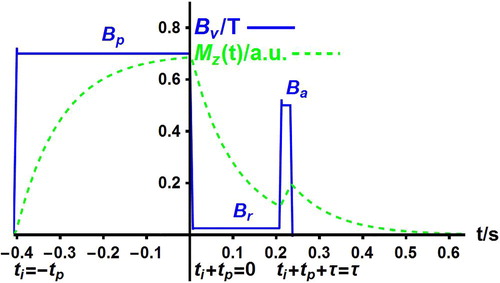
The PP sequence [Citation1] is a typical FFC sequence of successive different field values which is sketched in Figure . The PP sequence allows one to explore the evolution of the nuclear magnetisation at low field and to derive the intrinsic relaxation rates of the studied nuclei and their lifetimes in their different sites.
Figure 1. Basic cycle of the magnetic field (continuous line) in a pre-polarised (PP) sequence. The field
successively takes the polarisation value
for a polarisation time
, the relaxation value
for an evolution time
, the signal acquisition value
for an acquisition time
, and the zero value for a repetition delay taken to be equal to
. The nuclear magnetisation
(dotted line) in arbitrary units tends to its instantaneous equilibrium value
so that it evolves as the field
with some delay. The time origin is conveniently taken to be at the start of the evolution period
.
Turn to the description of the PP sequence and to the related theoretical expression of the evolution of the magnetisation column during this sequence. The applied magnetic field successively takes the polarisation value
, typically between 0.2 and 1 T, for a fixed polarisation duration
, the relaxation value
during the variable evolution time
, and the acquisition value
during the fixed acquisition time
taken to be somewhat longer than the delay
required to ensure field stability. Since relaxation at field
is investigated by varying
, the time origin is taken to be the start of the evolution period. The magnetisation column
at time
is calculated by successive applications of the operators
,
, and
. It reads
(19)
(19) The observed signal is the free induction decay (FID) obtained by applying a 90° pulse at the stabilised acquisition field
after the acquisition delay
. It is proportional to the total longitudinal magnetisation
. Finally, after recording the FID, the applied magnetic field
is switched off to zero during a fixed repetition delay
of the order of the polarisation duration
before repetition (cycling) of the sequence. The repetition delay is chosen so that the magnetisations of both sites are zero before the start of a new cycle. In Figure , note that the field
displays sudden jumps at times
,
,
and after the acquisition of the FID, though field ramps occur in practice. The magnetisations
,
remain constant across these ideal field jumps.
Assume that the polarisation period is longer than
, where
,
are the intrinsic relaxation times in the polarisation field
. Then, the magnetisation column
reaches its equilibrium value
at the end of the polarisation period so that
. Replacing
and
by their affine expressions in Equation (18) and setting
(20)
(20) Equation (19) simplifies to
(21)
(21) Replacing
and
by their expressions in Equation (14) with
(
) given by Equations (16) and (17),
can be rewritten as
(22)
(22) where the columns
,
are defined as
(23)
(23) with
(24)
(24) and
,
.
The NMR signal is proportional to
(25)
(25) where the coefficients
,
are defined as
(26)
(26) with
defined by Equation (9) and
given by Equation (24).
Turn to the limiting case . According to Equations (22) and (23), the column magnetisation becomes
(27)
(27) with the columns
(28)
(28) Then, the NMR signal is proportional to
(29)
(29) with the coefficients
(30)
(30) The expressions of the coefficients
can be simplified. Introducing the discriminant
, the coefficients
in Equation (30) can be rewritten as rational fractions in
. Replacing
by its expression in terms of
,
,
,
and using the equality
,
simplify to
(31)
(31) with
. Following Ruggiero et al. [Citation14], consider the evolution of the magnetisation of the hydrogen nuclei of water exchanging between intra- (
) and extra- (
) cellular compartments for the saturation recovery sequence. Setting
,
,
,
, according to Equations (1) and (4) of the Supporting Information of Ref. [Citation14], the coefficients of the decreasing exponentials
and
with the shorter (S) and longer (L) apparent relaxation times are
(32)
(32) and
, respectively. From Equation (31),
and
are respectively proportional to
and
with the same proportionality factor
. Thus, the changes of
with time of the PP sequence and saturation recovery sequence are just proportional at any evolution time
For immediate acquisition
, the difference between the two sequences is the dynamic range of
which decreases from
to
for the PP sequence and increases from 0 to
for the saturation recovery or non-polarised (NP) [Citation1] sequence. Since the magnetisation
is proportional to an NMR experimental signal, which is defined up to an arbitrary multiplicative factor,
and
should be considered as additional independent fit parameters when fitting the model of
of Equations (29) and (30) to experimental data, unless there is a relationship between
and
due to the experimental conditions.
4. Particular cases
Following McLaughlin and Leigh [Citation20], slow and fast exchange situations can be defined by comparing the effective exchange rate , the so-called ‘shutter-speed’ [Citation16], and the relaxation rate difference
defined as
(33)
(33) The slow and fast exchange situations are defined by the inequalities
and
, respectively. They depend on the field value
because the intrinsic relaxation rates
,
vary with the field.
4.1. Immediate acquisition 
4.1.1. Slow exchange limit in the relaxation field :
For , the fast and slow effective relaxation rates are
(34)
(34) According to Equations (7) and (34), we have
,
. The slow exchange condition leads to
so that
and
. Since
, according to Equation (24), we have
(35)
(35) Consequently, from Equations (27), (28), and (34), the magnetisations of sites A and B are
(36)
(36) Dropping all the terms with the factors
, these magnetisations reduce to
(37)
(37) Since
, the total magnetisation derived from Equation (36) is
(38)
(38) Except if
, for instance, when
,
reduces to the symmetric expression
(39)
(39) When
, the values of
,
,
, and
are obtained by permutation of the roles of A and B. Note that under the additional conditions
and
, the total magnetisation evolves as the sum of the magnetisations of sites without exchange.
4.1.2. Fast exchange limit in the relaxation field :
The fast exchange condition leads to the inequality . Setting
(40)
(40) the effective relaxation rates are
(41)
(41) Then, we have
,
,
,
, and
. From Equation (28), we get
(42)
(42) so that the site magnetisations are
(43)
(43) and the total magnetisation is
(44)
(44) The total magnetisation decays with the slow effective relaxation rate
given by Equation (41).
4.1.3. Site of scarce nuclei with high intrinsic relaxation rate
Assume that the population of site B is scarce, i.e. and
, with a high relaxation rate
. For instance, the situation occurs in liquid solutions when A corresponds to the solvent molecules in the bulk and B to solvent molecules bound to paramagnetic species or slowly rotating macromolecules. Then, as
, we have
. Then, the effective relaxation rates are
(45)
(45) The parameters defining the change-of-basis matrices
and
from Equation (10) with
are
,
,
. By neglecting terms in
and
, from Equations (27) and (28), the site magnetisations can be approximated as
(46)
(46) so that the total magnetisation is
(47)
(47)
The evolution of Equation (47) with
given by Equation (45) overlaps the time decays obtained above in the slow and fast exchange limits. Indeed, in the slow exchange case
,
in Equation (45) reduces to
, so that
obeys Equation (39) with negligible site B magnetisation. In the fast exchange limit
,
in Equation (45) takes the form
of Equation (41).
4.2. Delayed acquisition
4.2.1. Slow exchange limits in the relaxation and acquisition fields and :
Assume that the slow exchange condition also holds in the acquisition field
though the intrinsic relaxation rates are expected to have values lower than those in the relaxation field
since relaxation rates usually decrease as field increases. For
, as for the relaxation field
, we have
,
,
,
, and
. Then, dropping all the terms in factors of
or
, the columns
,
defined by Equations (23) and (24) reduce to
(48)
(48) According to Equation (22), we have
(49)
(49) and the total magnetisation reads
(50)
(50)
4.2.2. Slow exchange limit in the relaxation field and fast exchange limit in the acquisition field :
This situation may occur since relaxation rates usually decrease as field increases so that which is expected to be smaller than
, can become much smaller than
. For
, as in Section 4.1.1, we have
,
and
. As for the fast exchange limit in the relaxation field
studied in Section 4.1.2, setting
, the effective relaxation rates are
,
, so that we have
,
,
. Then, neglecting the terms with the factors
, the total magnetisation is given by
(51)
(51)
4.2.3. Fast exchange limits in the relaxation and acquisition fields and :
Since relaxation rates usually decrease as field increases, it is expected that the condition of fast exchange at field implies the analogous condition
of fast exchange at field
. As for the fast exchange limit in the relaxation field
studied in Section 4.1.2, setting
, the effective relaxation rates are
,
, so that we have
,
,
. The columns
,
are readily obtained from Equations (23) and (24). Using Equation (22), they yield the site magnetisations
(52)
(52) and the total magnetisation
(53)
(53)
4.2.4. Site of scarce nuclei with high intrinsic relaxation rates in the relaxation and acquisition fields and
Under the same conditions as in Section 4.1.3 and the hypothesis , the site magnetisations can be approximated as
(54)
(54) so that the total magnetisation is
(55)
(55) The
evolution of Equation (55) overlaps time decays obtained in the slow and fast exchange limits. For slow exchange in both fields
and
, Equation (55) becomes Equation (50) where the site B magnetisation terms in
and
are neglected. For fast exchange in both fields
and
, Equation (55) is identical to Equation (53).
As a rule, in the various cases of slow exchange in the fields and/or
, when either the intrinsic relaxation rate or the exchange rate is dominant for a given site, note that the
parameter giving the evolution of the site magnetisation is practically equal to the dominant term.
Finally, our formalism using the general evolution operator of the magnetisations of the exchanging sites can be easily applied to any FFC sequence.
5. Relaxometric exploration of systems
Information, that can be deduced from NMR relaxometry, depends on the values of ,
,
,
. Here, consider typical values of relaxation and residence times in biological systems. The residence time
of an intracellular water molecule is known to vary between 0.01 s for red blood cells to 100 s for xenopus ovocytes [Citation16]. These residence times should be compared with typical intrinsic relaxation times [Citation14]. Whatever the field, the
value is rather long, of the order of 1 s, in the extracellular medium, but can be considerably reduced by inclusion of paramagnetic contrast agents [Citation3–5,Citation11,Citation21]. On the other hand,
drops from 1 s to 30 ms when the field decreases from 0.25 T to 0.2 mT in mouse leg tissues. It should be emphasised that the detailed balance principle implies a decrease of the residence time
of an extracellular water molecule with the volume fraction of the extracellular space, so that
may become an order of magnitude shorter than
. Thus, the values of
,
,
,
range between a few milliseconds and a few seconds. They can be easily studied with standard NMR spectrometers, the pulse sequences of which make it possible to analyse the evolution of the nuclear magnetisation over times less than 0.1 ms.
The FFC-NMR investigation of dynamical processes of characteristic times between 1 ms and 1 s becomes problematic when the acquisition delay is not negligible with respect to the values of
,
,
,
,
,
. In practice, this delay incorporates the duration of the field ramp from
to
and the time required to ensure the
stability. It is only of a few milliseconds on a Stelar FFC relaxometer [Citation1], but can reach a few tens of milliseconds on an MRI scanner [Citation2].
The natural time unit of systems of nuclei undergoing chemical exchange is the shutter time
, or better
(56)
(56) which reduces to the common residence time
when the sites
and
have equal populations of nuclei. Therefore, the times
,
,
,
,
,
will be expressed in
units hereafter.
It is necessary to sample the total longitudinal magnetisation in the relaxation field
at both short and long
values in order to determine
and
, respectively. The application of a 90° pulse to measure
is only feasible from the moment when the acquisition field
is stable, that is at the end of a delay
after the fast jump of the field value
from
to a value near the acquisition value
which is reached by the rapid change of the current through the magnet coil. Then, the observed signal is proportional to
rather than
, where
is given by Equations (25) and (26), which can be used in the general case to derive the lifetimes and intrinsic relaxation rates of the sites at the relaxation field
. According to these equations, this derivation is only possible for a short delay
such as
is not significantly larger than unity. Otherwise, the signal vanishes and the relaxation information is lost. In particular, a bi-exponential decrease of the magnetisation can be reduced to an apparent mono-exponential decay if only one of the two factors
or
keeps a significant value.
Practically, the magnetisation decay with time can be fitted either by a single decreasing exponential or by a linear combination of two such exponentials corresponding in principle to the most general case of Equation (25). However, as shown below, the possibility of observing a bi-exponential decay occurs only in special cases because either exchange tends to lead to effective mono-exponential behaviour or the population of one site is largely dominant. A physico-chemical knowledge of the system of exchanging nuclei must be invoked to decide between these two cases. The
general expressions of Equations (25), (29), or its limiting expressions of Equations (39), (50), (51) should be used for bi-exponential decay. Simplified mono-exponential expressions, such as those of Section 4, can be used for mono-exponential relaxation.
Quite generally, bi-exponential relaxation is observable if the ratio derived from Equation (26) is neither too small nor too large, typically in the range
(57)
(57) Moreover, the effective relaxation rates
and
given by Equation (6) with
should differ significantly in order to be distinguishable from experimental data. This is all the more the case with increasing inaccuracy in the measurements and decreasing number of relaxation periods
. Typically, the ratio
should satisfy the inequality
(58)
(58) Assume that the relaxation field has a fixed value
. We will investigate the domain of the parameters
,
,
,
for which the total magnetisation has a bi-exponential decay. Introduce the population ratio
(59)
(59) In what follows, the optimal ideal situation of immediate acquisition
is considered first. The influence of delayed acquisition
is investigated later.
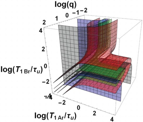
The domain of bi-exponential decay can be characterised by the only three independent dimensionless parameters ,
,
forming a three-dimensional space. In this space, the boundary surfaces of the bi-exponential domain, i.e.
(grey boundary) and 10 (blue boundary) with
, are shown in Figure as a function of the decimal logarithms of the three parameters. The domain is formed by two zones Z1 and Z2 between the grey and blue surfaces. More precise information is given in Figure where plane sections of Figure are displayed for different typical fixed q values. Within each of these plane sections, the frontiers of the dotted area are the traces of the above boundary surfaces corresponding to the conditions of Equation (57). Besides, the contours
and
appear as black and blue curves, respectively. They show that
ranges between
and
. They should be considered as matching the
and
axes when they are parallel and close to these axes. The areas corresponding to the ratio
in the intervals [1,2], [2,4], [4,12], [12,20], [20,
] are coloured in white, green, yellow, orange and red, respectively.
Figure 2. Bi-exponential relaxation domain, , in the space of logarithmic co-ordinates
with
,
,
for immediate signal acquisition
. This domain is defined by its boundaries
(grey contour) and
(blue contour). The surface contours
(green surface) and
(red surface) are also displayed (Colour online, B/W in print).

Figure 3. Bi-exponential relaxation areas, , (dotted zones) in the space of logarithmic co-ordinates
,
for immediate signal acquisition
and for the values 1, 0.2, 5, 0.01, 100 of the population ratio
. In the white zone corresponding to
< 2, observation of bi-exponential relaxation is difficult because of the proximity of
and
. Several intervals of the ratio
(coloured zones) are also displayed. For each
value, the point of co-ordinates
,
is represented by a black circle (Colour online, B/W in print).
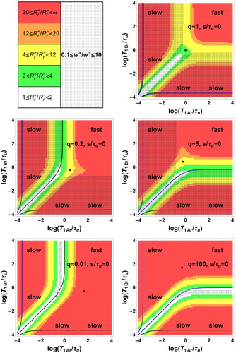
For , the bi-exponential behaviour occurs in two zones symmetric with respect to the principal diagonal with
, but not in the fast exchange area and in a narrow band around
.
For , there are two zones of observable bi-exponential relaxation: a dotted band parallel to the
axis corresponding to
with
and a dotted band parallel to the
axis corresponding to
on the left side of the black curve with
.
For , the figure is symmetric to the case
with respect to the principal diagonal
. The two zones of observable bi-exponential relaxation are a dotted band parallel to the
axis corresponding to
with
and a dotted band parallel to the
axis corresponding to
below the blue curve with
.
For , there is no intersection between the dotted and the coloured zones
indicating the absence of observable bi-exponential relaxation.
For , the figure is symmetric to the case
with respect to the principal diagonal
. There is no intersection between the dotted and coloured zones indicating the absence of observable bi-exponential relaxation.
Turn to an instrument with an acquisition delay . For an FFC-MRI scanner with
20–30 ms, consider residence times
,
of the order of 100–200 ms. Then, a typical acquisition delay is
. A delay time
leads to an attenuation of the observed signal. Besides this attenuation, the mono or bi-exponential decay of the total magnetisation leads to different qualitative changes. For the cases 4.2.3 and 4.2.4 of mono-exponential decay described by Equations (53) and (55), the attenuation is simply given by the factor
so that the inequality
should hold to keep a reasonable signal to noise ratio. The situation is similar for the limiting case 4.2.2 of fast exchange in field Ba and biexponential decay described by Equation (51). By contrast, for the limiting case 4.2.1 of slow exchange in field Ba and bi-exponential decay described by Equation (50), the relative weights of the two exponentials are differently affected. If
or
, the bi-exponential behaviour may reduce to a mono-exponential decay.
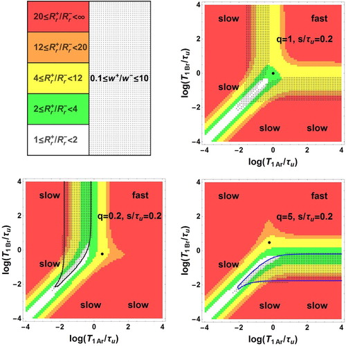
The loss of information brought by the delay time is illustrated in Figure for
1, 0.2, and 5, where the dotted areas correspond to the condition of bi-exponential decay of Equation (57). Comparing Figure (a–c) with the analogous Figure (a–c) relative to
, the areas corresponding to an observable bi-exponential decay of
are considerably reduced. For instance, for
1, the two symmetric large dotted zones of bi-exponential decay shrink to two symmetrical narrow areas. Moreover, the dotted band parallel to the
axis corresponding to
and the dotted band parallel to the
axis corresponding to
have disappeared for
= 0.2 and 5, respectively.
Figure 4. Bi-exponential relaxation areas, , (dotted zones) in the space of logarithmic co-ordinates
,
for delayed signal acquisition
and for the values 1, 0.2, 5 of the population ratio
. The white and coloured areas corresponding to value intervals of
are defined as in Figure . For each
value, the point of co-ordinates
,
is represented by a black circle (Colour online, B/W in print).
According to extensive previous studies [Citation15], the bi-exponential situation described by the present formalism is likely to occur frequently in biological tissues because the extra- and intra-cellular water molecules have comparable populations. For instance, the extra-cellular/intra-cellular water ratio is about 1 for blood and brain white matter. In many tissues, it ranges from 0.1 (muscle) to 20 (tumour rim). Moreover, by adding MRI contrast agents at various concentrations into cell suspensions [Citation14,Citation17], the intrinsic relaxation rate of the water protons of the extracellular medium can be significantly increased, making it possible to extract the intrinsic intracellular relaxation rate and the water residence lifetimes in both intra- and extra-cellular compartments by applying the present theory if the acquisition delay is short enough.
The influence of the acquisition delay on the best fit values of residence times and intrinsic relaxation times is illustrated now by simulating a very-low-field FFC-MRI investigation of a tumour tissue of a mouse leg [Citation14]. Indeed, prototypes of FFC-MRI scanners and FFC-NMR relaxometers operating down to 2 are under development within the framework of the European project IDentIFY. In a tissue, at a given relaxation field
, a water molecule basically goes back and forth between the intracellular
space with intrinsic longitudinal time
during a residence time
and the extracellular
space with intrinsic longitudinal time
during a residence time
. The population fractions are assumed to be
and
since
, denoted as
in Ref. [Citation14], ranges between 0.14 and 0.30. Since the intracellular lifetime
ranges between 0.48 and 1.44 s, we assume
= 800 ms and
= 200 ms. Below 0.2 mT, according to Figure of Ref. [Citation14] and to Fig. S2 of the related Supporting Information,
and
are expected to be of the order of a few tens and a few hundreds of ms, respectively. For simulation purpose, at
= 10
, we take extrapolated values
= 20 ms and
= 400 ms. The initial proton magnetisation is assumed to have the equilibrium value in the polarisation field
= 100 mT. The acquisition field is
= 60 mT, in which the estimates of the intrinsic relaxation times are
= 150 ms and
= 2000 ms. Finally, the acquisition delay has a typical value
= 20 ms as in an MRI scanner built by Lurie et al. [Citation2,Citation7–9]. Thus,
is not negligible with respect to both
and
.
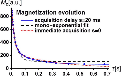
Applying the PP sequence of Figure , the evolution of the total magnetisation of the water protons is simulated for the above input parameter values according to Equation (25) which accounts for the acquisition delay. The simulated magnetisation values shown by dots in Figure were obtained for 24 exponentially spaced values of the evolution period
, ranging between 2 and 700 ms. As in a real experiment, each
value is affected by a random error assumed to be here of ±1%. Then, the best fit independent parameters
,
,
,
entering the magnetisation
in Equation (25) are expected to deviate from the ‘true’ input values
= 0.2,
= 200 ms,
= 20 ms,
= 400 ms. Even for the present small simulated ‘experimental’ uncertainties and despite the excellent agreement between the continuous fitted function
and the simulated data shown in Figure , several best-fit parameters
= 0.235,
,
= 19.8 ms,
= 146 ms are significantly different from the input values. In particular, the best-fit residence times have very large values so that there is practically no water exchange. Now, following Ruggiero et al. [Citation14], assume that the extracellular medium is similar to Matrigel and has the known value
= 400 ms obtained in Matrigel from independent FFC-NMR measurements. Under these conditions, we obtain
= 0.195 ± 0.01,
= 209 ± 18 ms,
= 20.3 ± 0.4 ms in very good agreement with the input values and still an excellent agreement between the continuous fitted function
and the simulated data as shown in Figure . Note that the simulated data cannot be reproduced by the mono-exponential fit represented by the dashed curve in Figure .
Figure 5. Typical bi-exponential time decay of the water proton magnetisation of a tumour tissue of a mouse leg at body temperature in the relaxation field = 10
of an FFC-MRI scanner. Water molecule basically goes back and forth between the intracellular space and the extracellular space. The discrete dots are the simulated data corresponding to
in Equation (25) with realistic exchange and relaxation input parameters (see text) for an acquisition delay
= 20 ms with random magnetisation errors of ±1%. The superimposed continuous curves are the excellent fits of
to the previous simulated data (see text). The dashed curve is the unsuccessful mono-exponential relaxation function fitted to the simulated data. The dotted curve is the poor fit of
(
) in Equation (29) to the simulated data.
Turn to the influence of the acquisition delay on the best-fit parameters. Here, the simulated data are still those which were previously obtained by using the magnetisation of Equation (25) with acquisition delay
= 20 ms, but the fitted function is the magnetisation
of Equation (29) with immediate acquisition
= 0. Setting
= 400 ms, the best-fit parameters
= 0.242,
= 1650 ms,
= 19 ms are in strong disagreement with the input values and lead to a fitted function
, represented in Figure by a dotted curve which also strongly departs from the simulated data. For
= 0, even if the amplitude of
is considered as an additional adjustable parameter through an additive term
, the fit agreement is not improved. This simple example shows that the influence of the acquisition delay on the best-fit parameters of the magnetisation expressions should be carefully examined in systems with bi-exponential decay as soon as it somewhat affects the observed magnetisation.
Finally, recent theoretical developments in the analysis of multi-exponential relaxation data [Citation22] should facilitate the precise determination of the physico-chemical parameters involved in systems of nuclear spins undergoing chemical exchange.
6. Conclusion
We have presented a general formalism for describing the evolution of the magnetisations of populations of nuclei exchanging between two sites after an FFC sequence. In the case of the PP sequence, we have derived general expressions of the magnetisation decay and provided simple formulas in the slow and fast exchange limits, and in the case of a site of scarce nuclei with high intrinsic relaxation rate. We have shown that a bi-exponential decay is only observable if both site populations are comparable and if the exchange rates are slower than or comparable to the absolute difference of intrinsic relaxation rates. We have given analytic expressions of the loss of information due to the finite acquisition delay. We have shown that the acquisition delay can strongly affect the fitted values of the populations, residence times, and intrinsic relaxation times of the sites in the case of bi-exponential relaxation.
Disclosure statement
No potential conflict of interest was reported by the authors.
Additional information
Funding
References
- G. Ferrante and S. Sykora, Adv. Inorg. Chem. 507, 405 (2005). doi: 10.1016/S0898-8838(05)57009-0
- D.J. Lurie, S. Aime, S. Baroni, N.A. Booth, L.M. Broche, C.-H. Choi, G.R. Davies, S. Ismail, D.Ó. Hógáin and K.J. Pine, C. R. Phys. 11, 136 (2010). doi: 10.1016/j.crhy.2010.06.012
- L. Banci, I. Bertini and C. Luchinat, Nuclear and Electron Relaxation: The Magnetic Nucleus-Unpaired Electron Coupling in Solution (VCH, Weinheim, 1991).
- I. Bertini, C. Luchinat and G. Parigi, Solution NMR of Paramagnetic Molecules (Elsevier, Amsterdam, 2001).
- C.S. Bonnet, P.H. Fries, S. Crouzy and P. Delangle, J. Phys. Chem. B 114, 8770 (2010). doi: 10.1021/jp101443v
- A.L. Rollet, S. Neveu, P. Porion, V. Dupuis, N. Cherrak and P. Levitz, Phys. Chem. Chem. Phys. 18, 32981 (2016). doi: 10.1039/C6CP06012A
- D. Kruk, M. Wojciechowski, Y.L. Verma, S.K. Chaurasia and R.K. Singh, Phys. Chem. Chem. Phys. 19, 32605 (2017). doi: 10.1039/C7CP06174A
- K. Venu, V.P. Denisov and B. Halle, J. Am. Chem. Soc. 119, 3122 (1997). doi: 10.1021/ja963611t
- E. Persson and B. Halle, Proc. Natl. Acad. Sci. 105, 6266 (2008). doi: 10.1073/pnas.0709585105
- E. Ravera, G. Parigi, A. Mainz, T.L. Religa, B. Reif and C. Luchinat, J. Phys. Chem. B 117, 3548 (2013).
- D.Ó. Hógáin, G.R. Davies, S. Baroni, S. Aime and D.J. Lurie, Phys. Med. Biol. 56, 105 (2011). doi: 10.1088/0031-9155/56/1/007
- L.M. Broche, S.R. Ismail, N.A. Booth and D.J. Lurie, Magn. Reson. Med. 67, 1453 (2012). doi: 10.1002/mrm.23117
- L.M. Broche, G.P. Ashcroft and D.J. Lurie, Magn. Reson. Med. 68, 358 (2012). doi: 10.1002/mrm.23266
- M.R. Ruggiero, S. Baroni, S. Pezzana, G. Ferrante, S. Geninatti Crich and S. Aime, Angew. Chem. Int. Ed. 57, 7468 (2018). doi: 10.1002/anie.201713318
- C.S. Landis, X. Li, F.W. Telang, P.E. Molina, I. Palyka, G. Vetek and C.S. Springer, Jr., Magn. Reson. Med. 42, 467 (1999). doi: 10.1002/(SICI)1522-2594(199909)42:3<467::AID-MRM9>3.0.CO;2-0
- C.S. Springer, Jr., X. Li, L.A. Tudorica, K.Y. Oh, N. Roy, S.Y-C. Chui, A.M. Naik, M.L. Holtorf, A. Afzal, W.D. Rooney and W. Huang, NMR Biomed. 27, 760 (2014). doi: 10.1002/nbm.3111
- E. Gianolio, G. Ferrauto, E. Di Gregorio and S. Aime, Biochim. Biophys. Acta 1858, 627 (2016). doi: 10.1016/j.bbamem.2015.12.029
- G.J. Béné, Helv. Phys. Acta 61, 572 (1988).
- H.M. McConnell, J. Chem. Phys. 28, 430 (1958). doi: 10.1063/1.1744152
- A.C. McLaughlin and J.S. Leigh, Jr., J. Magn. Reson. 9, 296 (1973).
- J. Kowalewski and L. Mäler, Nuclear Spin Relaxation in Liquids: Theory, Experiments, and Applications (Taylor & Francis, New York, 2006).
- O.V. Petrov and S. Stapf, J. Magn. Reson. 279, 29 (2017). doi: 10.1016/j.jmr.2017.04.009