On the use of reduced-density matrices for the semi-automatic assignment of vibrational states

ABSTRACT

The use of one- and two-mode reduced-density matrices (RDM), ${\mathrm{\Gamma }}_1(q_i{}^{\prime },q_i)$ and ${\mathrm{\Gamma }}_2(q_i{}^{\prime },q_j{}^{\prime },q_i,q_j)$, respectively, and in particular the use of their diagonal elements, ${\mathrm{\Gamma }}_1(q_i,q_i)$ and ${\mathrm{\Gamma }}_2(q_i,q_j,q_i,q_j)$, is suggested for the assignment of normal-mode-like quantum numbers to variationally computed vibrational wave functions of semirigid molecules when the computation is based on a nuclear-motion Hamiltonian expressed in curvilinear internal coordinates $q_i$. The use of RDMs for the semi-automatic assignment of vibrational states is tested on the H${}_2{}^{16}$O molecule, whereby about the first 250 states, in the energy range of 0–25,000 cm⁻¹, are assigned. The proposed semi-automatic assignment procedure takes advantage of the fact that (a) for semirigid molecules it is often possible to define internal coordinates which mimick normal coordinates defined by the harmonic counterparts of the anharmonic vibrations, (b) overlaps between already assigned and yet unassigned RDMs provide outstanding and often unambiguous suggestions for the quantum numbers, and (c) an energy-decomposition scheme helps to decide among possible assignment possibilities suggested by the computed density overlaps.

GRAPHICAL ABSTRACT

Keywords:

• Wave-function analysis
• one- and two-mode reduced-density matrices
• vibrational assignment
• quantum numbers

1. Introduction

In the fourth age of quantum chemistry [1] the variational computation and subsequent characterisation of a large number of rovibronic states of polyatomic molecular systems has become increasingly realistic. Symmetry, in the form of irreducible representations, is an exact information about the rovibrational states if the correct group is employed during the nuclear-motion computation. The quantum number J, corresponding to overall rotation, is an exact quantum number in a field-free case; thus, J is available from all variational quantum-chemical computations concerning nuclear dynamics to characterise (label) the computed states. Parity, p, is another piece of exact information about the computed rovibrational states. Note that parity information can sometimes be connected to vibrational quantum numbers (vide infra).

When the Eckart–Watson (EW) Hamiltonian [2–4], a Hamiltonian based on the well-defined concepts of a single reference structure and normal coordinates, is employed for the variational computation of (ro)vibrational states, it is often appropriate to use point-group symmetry and the corresponding irreducible representations to label the states. If, however, the rovibrational Hamiltonian is based on the use of internal coordinates, molecular symmetry (MS) groups and their (often many-dimensional) irreducible representations should be used to label the rovibrational states (correlation tables can be employed to deduce the correct MS symmetry labels if a group of lower symmetry was employed during the computation). Some of the nuclear-motion codes are able to provide symmetry labels [5–8] characterising the computed states. Nevertheless, a lot of practical applications and the detailed spectroscopic characterisation of the internal motions of a molecule require the assignment of the computed vibrational states with quantum numbers associated with the 3N−6 vibrational degrees of freedom of an N-atomic nonlinear molecule (see ref. [9] and references cited therein; rotations are usually labelled with the $\left[J{K}_a{K}_c\right]$ asymmetric-top quantum number triplet [10]). There are no exact quantum numbers describing the anharmonic vibrations of molecular systems. The two most common choices of approximate vibrational quantum numbers are based on the concept of normal [11] and local [12,13] modes. In general, for semirigid molecules it is more usual to apply the 3N−6 normal-mode quantum numbers [9,14,15]. This is a successful and time-proven approach for lower-energy states of semirigid molecules. When a code based on the EW Hamiltonian [2–4] is employed for the variational computation of the vibrational states and the one-dimensional basis functions are based on Hermite polynomials, the computation provides a natural way for the assignment of the vibrational states. This type of basis set projection technique underpins, for example, the normal-mode decomposition (NMD) technique [16]. Curvilinear coordinates are much more suitable to treat vibrational motions than normal coordinates [17–19]. When the rovibrational Hamiltonian is based on curvilinear internal coordinates, assigning quantum numbers to the computed vibrational states is not trivial and no universal, black-box-type method is available. Labeling of computed eigenstates is an important step toward understanding nuclear dynamics, allowing its eventual control. Let us recall the few techniques developed for the assignment of variationally computed vibrational states.

The simplest method, which can be called energy decomposition, is based on the use of the energy dependence of the computed vibrational eigenenergies (fundamentals, overtones, and combination bands) on the normal-mode (harmonic oscillator) energies and their ‘exact’ quantum numbers. The applicability of this technique is mostly limited to low-energy states of semirigid molecules. As an alternative, one can add artificial corrections to the potential energy surface (PES) along certain coordinates and see which eigenvalues change and by how much and deduce information about the vibrational character of the state this way. Obviously, these two techniques do not require the availability of wave functions to assign quantum numbers to the computed states but their range of applicability is rather limited.

As most of the codes developed for the solution of the nuclear-motion Schrödinger equation are able to provide not only eigenvalues but eigenfunctions, as well [1], the wave functions can be employed to obtain additional important non-exact, qualitative information about the computed (ro)vibrational eigenstates. The next three techniques discussed require the availability of vibrational wave functions. First, two-dimensional (2D) cuts of vibrational wave functions, along all coordinate pairs, and counting the nodes by visual inspection often give valuable information about the excitations characterising the computed states. The 2D cuts are particularly useful for states of more or less pure stretching or bending character. However, plots cannot be used to assign quantum numbers to strongly mixed states without significant manipulation. It is also hard to identify multiply excited states by visual inspection even if such states were fairly harmonic. Thus, while the node-counting method appears to be useful for small systems and low excitation energies, see, for example, Refs. [9], [20], and [21], it quickly becomes impractical and prone to errors for larger systems, when the number of vibrational degrees of freedom and the number of possible mode combinations increase [22]. Second, expectation values of certain parameters may also provide useful information about the excitation characteristics of certain vibrational states. The applicability of the expectation values of, for example, geometric parameters, are based on the anharmonicity of the true PES. In the already mentioned technique, the NMD [16] of variational vibrational wave functions, the variationally computed, normalised vibrational wave functions, ${\psi }_i$, are characterised by the square of their overlaps with the normalised harmonic-oscillator basis functions, ${\phi }_v^{\mathrm{HO}}$, expressed in terms of normal coordinates corresponding to the actual PES. Finally, as alternatives to the full-dimensional wave-function projection technique, perturbative approaches may also enable harmonic-oscillator-based assignments without the need for explicitly computing the eigenvectors [23,24]. As demonstrated by Yu et al. [24], with appropriate coordinate definitions and a set of specific perturbation operators, the perturbative approach can successfully provide normal-mode quantum numbers for vibrational states of molecules exhibiting even large-amplitude motions.

The present work focuses on a novel assignment technique based on the use of one- and two-mode reduced-density matrices (RDM). This approach was first used in our study of the rovibrational states of the vinyl radical [25] but there no detailed account of the technique was given. In Ref. [25] we plotted only the diagonal elements of the RDM matrices (${\mathrm{\Gamma }}_1^{\mathrm{D}}$ and ${\mathrm{\Gamma }}_2^{\mathrm{D}}$), representing the modal wave-function density, and visually assigned the states based on kinks in the density plots. The method proved to be successful and straightforward to use for many states, even though information about the sign changes of the wave function at the nodes is not directly available when the densities are plotted. What we observed in Ref. [25] is that, compared to the simple wave-function visualisation and node-counting method, the visualisation of the densities does not require choosing any reference coordinate configuration, it integrates out many misleading structural details of the wave function, and it describes each state by only a small number of compact density plots. Besides these convenient properties of this approach we also observed that the pattern of the density of a particular excitation tends to be very regular across all the vibrational states characterised by this excitation. Therefore, a given excitation can be determined by its ‘density shape’. Actually, this is a key idea behind the current study, as this means that one can compare overlaps of the mode densities in a semi-automatic way. Another improvement over Ref. [25] is the possibility of directly observing the sign alterations at nodes by plotting the full 2D picture of the one-mode RDM, ${\mathrm{\Gamma }}_1$. Moreover, if a coordinate system is chosen such that each normal mode is described by basically one internal coordinate, the need for ${\mathrm{\Gamma }}_2^{\mathrm{D}}$ is eliminated and one could even develop an automatic assignment based on ${\mathrm{\Gamma }}_1^{\mathrm{D}}$ plots, without the need to probe each new ${\mathrm{\Gamma }}_2^{\mathrm{D}}$ shape for the coupled coordinate pair.

During this study we use water, in particular the H${}_2{}^{16}$O isotopologue [15], as our test molecule to investigate the capabilities of RDMs for the assignment of quantum numbers to a large number of vibrational states. We do this since detailed normal-mode labels have been reported [20] for a large number of vibrational states of H${}_2{}^{16}$O, up to about 25 000 cm⁻¹. The following characteristics of the vibrational states of H${}_2{}^{16}$O complicate the assignment procedure: (a) the vibrations of water show both local- and normal-mode behaviour even at relatively low energies, (b) above a certain energy water ceases to remain a semirigid molecule, and (c) water is characterised by a low barrier to linearity, around 11,000 cm⁻¹ [26], and thus quantum monodromy [27] must be considered for this molecule.

2. Reduced-density matrices

To at least partially remedy problems associated with the usual assignment procedures based on the visual inspection of wave functions and node counting, hereby we explore the application of one- and two-mode reduced-density matrices, ${\mathrm{\Gamma }}_1$ and ${\mathrm{\Gamma }}_2$, respectively, for assigning computed vibrational states. The quantities ${\mathrm{\Gamma }}_1$ and ${\mathrm{\Gamma }}_2$ used in this study extensively are defined as follows: (1) $\begin{array}{rl}{\mathrm{\Gamma }}_1(q_i{}^{\prime },q_i)& =\int \mathrm{d}{q}_1\dots \mathrm{d}{q}_{i-1}\mathrm{d}{q}_{i+1}\dots \mathrm{d}{q}_N\\ & \times {\mathrm{\Psi }}^{\ast }(q_1,\dots ,q_{i-1},q_i{}^{\prime },q_{i+1},\dots ,q_N)\\ & \times \mathrm{\Psi }(q_1,\dots ,q_{i-1},q_i,q_{i+1},\dots ,q_N)\end{array}$(1) and (2) $\begin{array}{rl}& {\mathrm{\Gamma }}_2(q_i{}^{\prime },q_j{}^{\prime },q_i,q_j)\\ & =\int \mathrm{d}{q}_1\dots \mathrm{d}{q}_{i-1}\mathrm{d}{q}_{i+1}\dots \mathrm{d}{q}_{j-1}\mathrm{d}{q}_{j+1}\dots \mathrm{d}{q}_N\\ & \times {\mathrm{\Psi }}^{\ast }(q_1,\dots ,q_{i-1},q_i{}^{\prime },q_{i+1},\dots ,q_{j-1},q_j{}^{\prime },q_{j+1},\dots ,q_N)\\ & \times \mathrm{\Psi }(q_1,\dots ,q_{i-1},q_i,q_{i+1},\dots ,q_{j-1},q_j,q_{j+1},\dots ,q_N),\end{array}$(2) while their diagonal elements are (3) $\begin{array}{rl}{\mathrm{\Gamma }}_1^{\mathrm{D}}\left(q_i\right)& ={\mathrm{\Gamma }}_1(q_i,q_i)\\ & =\int \mathrm{d}{q}_1\dots \mathrm{d}{q}_{i-1}\mathrm{d}{q}_{i+1}\dots \mathrm{d}{q}_N\\ & \times {\mathrm{\Psi }}^{\ast }(q_1,\dots ,q_N)\mathrm{\Psi }(q_1,\dots ,q_N)\end{array}$(3) and (4) $\begin{array}{rl}{\mathrm{\Gamma }}_2^{\mathrm{D}}(q_i,q_j)& ={\mathrm{\Gamma }}_2(q_i,q_j,q_i,q_j)\\ & =\int \mathrm{d}{q}_1\dots \mathrm{d}{q}_{i-1}\mathrm{d}{q}_{i+1}\dots \mathrm{d}{q}_{j-1}d{q}_{j+1}\dots \mathrm{d}{q}_N\\ & \times {\mathrm{\Psi }}^{\ast }(q_1,\dots ,q_N)\mathrm{\Psi }(q_1,\dots ,q_N).\end{array}$(4) The ${\mathrm{\Gamma }}_1^{\mathrm{D}}\left(q_i\right)$ and ${\mathrm{\Gamma }}_2^{\mathrm{D}}(q_i,q_j)$ quantities actually represent the wave-function density along a given coordinate or a coordinate pair. These quantities do not show the change of the sign of the wave function at the nodes. However, it turns out that the nodal structure is very nicely matched by kinks in the density and for many vibrational states the density information is completely sufficient for a successful assignment.

The nodal structure is revealed by the full ${\mathrm{\Gamma }}_1(q_i{}^{\prime },q_i)$ matrix, whereby the change of the sign of the wave function induces a sign change in the density matrix when moving along a coordinate through a wave-function node.

The structure of the density plots, formed by the mentioned ‘kinks’, depends only moderately on the computational grid employed and a much smaller number of density plots needs to be generated for an assignment than the number of wave-function projections needed during node counting. Density plots tend to be very regular even in multimodal excited states, helping semi-automatic assignment procedures (vide infra). Furthermore, a particular advantage of ${\mathrm{\Gamma }}_1^{\mathrm{D}}$ and ${\mathrm{\Gamma }}_2^{\mathrm{D}}$ is that positive- and negative-parity vibrational states are characterised by extremely similar plots (even more so than for the wave functions), helping considerably their pairing. This proved to be useful in the case of the assignment of the vibrational states of the vinyl radical, characterised by a pronounced large-amplitude tunnelling behaviour [25].

3. Computational details

The vibrational eigenstates of H${}_2{}^{16}$O were computed in this study with the in-house nuclear-motion code GENIUSH [17,18], where GENIUSH stands for a general (GE), numerical (N) rovibrational programme employing curvilinear internal (I) coordinates and user-specified (US) Hamiltonians (H). Within GENIUSH the wave function is represented on a full or reduced-dimensional grid by using the discrete variable representation (DVR) technique [28,29] and the resulting large-scale eigenvalue problem is solved iteratively by the Lanczos algorithm [30]. The latest version of the GENIUSH code utilises the molecular symmetry (MS) group in the vibration-only mode of computation, yielding proper symmetry labels for the vibrational eigenstates [6].

In this study the internal coordinates of the water molecule were chosen as either the valence coordinates, $R_1$, $R_2$, and ϑ, as shown in Figure 1, or their symmetrised combination $(R_1+R_2)$, $(R_1-R_2)$, and ϑ. Details about the DVR grid applied is given in Table 1.

Figure 1. The simple valence internal coordinates of the water molecule, $R_1$, $R_2$, and ϑ, used during this study.

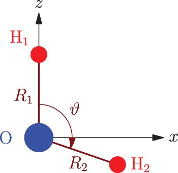
Table 1. Details of the computational grid used in this study for both the valence and the symmetrised valence internal coordinate systems.

	$R_1$	$R_2$	ϑ	$(R_1+R_2)$	$(R_1-R_2)$	ϑ
DVR type	Hermite	Hermite	Legendre*	Hermite	Hermite	Legendre
Range	0.51–2.15	0.51–2.15	10.0–179.7	1.25–3.00	$-1.06$–+1.06	10–179.7
No. of elementary DVR points	200	200	200	300	300	300
No. of PO-DVR points	40	40	55	90	90	120
Ref. conf.	0.95782	0.957 82	104.5	1.915 64	0.0	104.5

Notes: See Figure 1 for the definition of the valence coordinates. PO-DVR means potentially-optimised DVR using the given reference configuration. The ranges for the internuclear distances ($R_i$) and the angle (ϑ) are in Å and degrees, respectively. ${}^{\ast }$The DVR coordinate is not ϑ, but cos$\left(\vartheta \right)$.

The PES employed in this study is taken from Ref. [31]. This choice facilitates the comparison of the computed states with those of Ref. [20] as well as to the so-called IUPAC water data of Ref. [15].

4. A semi-automatic assignment procedure

While the semi-automatic assignment procedure developed during this study works the same way for all molecules, the discussion given here concentrates on the chosen test molecule, H${}_2{}^{16}$O. For H${}_2{}^{16}$O, the energy-decomposition technique can be expressed as (5) $E(v_1,v_2,v_3)=v_1{\nu }_1+v_2{\nu }_2+v_3{\nu }_3,$(5) where $v_1$, $v_2$, and $v_3$ (often given as $\left(v_1{v}_2{v}_3\right)$) and ${\nu }_1$, ${\nu }_2$, and ${\nu }_3$ are the vibrational quantum numbers and the vibrational fundamentals corresponding to the so-called symmetric stretch, bend, and antisymmetric stretch normal modes of H${}_2{}^{16}$O, respectively.

For H${}_2{}^{16}$O, the method of energy decomposition works extremely well for eigenenergies up to about 12,000 cm⁻¹ and no additional information is required to label these vibrational states. We note that at 12,000 cm⁻¹ the stretching motions of water are already much more accurately described by a local-mode rather than a normal-mode picture [32]. Above this energy, the density of states increases and there are often several candidate states for a given set of vibrational quantum numbers. Additional information about the vibrational state is therefore needed. Note that for the vibrational states of H${}_2{}^{16}$O the parity of the state is given by $(-1{)}^{v_3}$. In general, such relations may not exist and even when normal-mode labels can be allocated based on energy decomposition (or any other scheme), their physical relevance can often be questioned.

Since the results of the present assignment procedure are to be compared to the labels provided in Ref. [20], it is worth recalling some of the relevant results of Ref. [20]. Assignment of vibrational quantum numbers to levels with large $v_2$ values proved to be particularly difficult. In Ref. [20] all VBOs up to 26,500 cm⁻¹ could be labelled; however, above this energy the proportion of labelled VBOs drops steadily with increasing energy. It is certainly feasible to provide labels to vibrational states above 26,500 cm⁻¹ but this was not tried in a systematic way. Despite the drop in the number of assigned VBOs with energy, in Ref. [20] labels were provided for states with low values of $v_2$ all the way to dissociation.

In the present study we employed two basically similar assignment schemes, one using the simple valence internal coordinates $R_1$, $R_2$, and ϑ (see Figure 1), while the other uses the symmetrised coordinates $(R_1+R_2)$, $(R_1-R_2)$, and ϑ. For the former, ‘local-mode-like’ scheme we compare ${\mathrm{\Gamma }}_2^{\mathrm{D}}(R_1,R_2)$ and ${\mathrm{\Gamma }}_1^{\mathrm{D}}\left(\vartheta \right)$ matrices between states, while in the latter, ‘normal-mode-like’ case we compare the ${\mathrm{\Gamma }}_1((R_1+R_2){}^{\prime },(R_1+R_2\left)\right)$, ${\mathrm{\Gamma }}_1(\vartheta {}^{\prime },\vartheta )$, and ${\mathrm{\Gamma }}_1((R_1-R_2){}^{\prime },(R_1-R_2\left)\right)$ matrices (in principle, the diagonal elements ${\mathrm{\Gamma }}_1^{\mathrm{D}}(R_1+R_2)$, ${\mathrm{\Gamma }}_1^{\mathrm{D}}\left(\vartheta \right)$, and ${\mathrm{\Gamma }}_1^{\mathrm{D}}(R_1-R_2)$ may suffice, but, as we show in the following section, in many cases to distinguish a node from a simple density kink the full 1-mode RDM is required).

For proper comparison of the states we can take advantage of the fact that densities sum up to one, (6) $\int \mathrm{d}q{\mathrm{\Gamma }}_1^{\mathrm{D}}\left(q\right)=1;$(6) thus, we renormalise the densities so that (7) $\int \mathrm{d}q{\left({\mathrm{\Gamma }}_1^{\mathrm{D}}\left(q\right)\right)}^{\ast }{\mathrm{\Gamma }}_1^{\mathrm{D}}\left(q\right)=1$(7) and analogously for the other relevant quantities, ${\mathrm{\Gamma }}_2^{\mathrm{D}}(q_i,q_j)$ and ${\mathrm{\Gamma }}_1(q{}^{\prime },q)$. With quantities renormalised this way we can compare them between states with the resulting overlap ranging from zero to one.

Let us show how the proposed semi-automatic assignment procedure works via a couple of examples. To avoid obvious misassignments, a trivial excitation aufbau principle is followed in our semi-automatic assignment procedure, whereby the density-overlap-based assignments are taken from a pool of ‘allowed’ states. The set of allowed states is updated at each step starting from assigning $\left(000\right)$ to the first (ground) state. Then, the second state can only be one of the $\left(100\right)$, $\left(010\right)$, or $\left(001\right)$ states, i.e. one of the fundamentals. Assuming that the second state has been assigned to $\left(010\right)$, based on RDM plots (which is actually the correct assignment), the set of allowed states for the next vibrational state becomes $\left(100\right)$, $\left(020\right)$, and $\left(001\right)$. The states $\left(110\right)$ or $\left(011\right)$ should not be taken into account here since such states can come only after the states $\left(100\right)$ or $\left(001\right)$ have been found. The set of allowed states thus remains relatively compact and helps substantially in the assignment process, especially in difficult cases.

Once all the fundamental modes, in the case of H${}_2{}^{16}$O $\left(100\right)$, $\left(010\right)$, and $\left(001\right)$, have been assigned, an approximate energy is computed for each of the allowed states based on the single-mode energies and the allowed states are sorted accordingly. The new order of allowed states is not always fully relevant, particularly for higher combination states, but definitely helps in the case of problematic assignments. This energy-decomposition scheme basically follows the accounting of vibrational states based on the polyad number of H${}_2{}^{16}$O [15].

An important criterion for the assignment within our procedure remains the visual inspection of density plots. Nevertheless, in this study of the vibrational states of the water molecule, when simple valence coordinates are used, the visual inspection was basically unnecessary during the analysis of the vast majority of the states, as the assignments suggested by the density overlaps and the energy-decomposition scheme were mostly unambiguous and correct. The proper assessment of the density plots become, however, inevitable for some of the states, where the automatic energy decomposition scheme is not sufficient in itself.

We also would like to stress that reduced-density-matrix plots have a limited applicability since the density structures are often too complicated to distinguish nodes, especially in the ${\mathrm{\Gamma }}_2^{\mathrm{D}}(R_1,R_2)$ plots in the case of H${}_2{}^{16}$O (clear-cut cases are shown in Figure 3). For such non-trivial density shapes the overlap-based comparisons should definitely supplement visual inspection.

The actual script written to provide a semi-automatic procedure for the assignment of the vibrational states of water using densities expressed in valence internal coordinates can be summarised as follows. Let us introduce the canonical order of the vibrations, $\left(v_1{v}_2{v}_3\right)$, for water. We start by assigning state #1 with $\left(000\right)$ and store the corresponding mode densities ${\mathrm{\Gamma }}_2^{\mathrm{D}}(R_1,R_2)$ and ${\mathrm{\Gamma }}_1^{\mathrm{D}}\left(\vartheta \right)$ with their corresponding quantum numbers $\left(00\right)$ and 0, respectively. Then, a new set of allowed states is generated. For state #2 the ${\mathrm{\Gamma }}_2^{\mathrm{D}}(R_1,R_2)$ density has almost unit overlap with that of state #1, while the ${\mathrm{\Gamma }}_1^{\mathrm{D}}\left(\vartheta \right)$ density exhibits a new structure. This immediately suggests that the correct assignment of state #2 is $\left(010\right)$. Since this label is among the allowed labels, state #2 receives this assignment and the new density ${\mathrm{\Gamma }}_1^{\mathrm{D}}\left(\vartheta \right)$ is stored together with a quantum number $v_2=1$. The procedure continues in an analogous way until the desired number of states received an assignment. The assignment procedure for the system with the symmetrised valence coordinates differs only in the type and the number of densities that are being compared and stored. In the present case of H${}_2{}^{16}$O, we found advantageous to set the threshold for density similarities at 0.9, though the vast majority of successfully assigned states had density overlaps as high as 0.99.

Figure 2. Plots corresponding to ${\mathrm{\Gamma }}_1^{\mathrm{D}}\left(\vartheta \right)$ (left column) and ${\mathrm{\Gamma }}_2^{\mathrm{D}}(R_1,R_2)$ (right column) diagonal reduced-density-matrix elements of selected vibrational states of H${}_2{}^{16}$O [between state #7 (1 1 0) and #14 (0 0 2)], computed using the simple valence coordinates $R_1$, $R_2$, and ϑ (Figure 1). The radial coordinates are in bohr, the angular one is in degrees.

Figure 3. Plots corresponding to ${\mathrm{\Gamma }}_1^{\mathrm{D}}\left(\vartheta \right)$ (left column) and ${\mathrm{\Gamma }}_2^{\mathrm{D}}(R_1,R_2)$ (right column) diagonal reduced-density-matrix elements of selected vibrational states of H${}_2{}^{16}$O [between states #28 (3 0 0) and #159 (5 1 1)], computed using the simple valence coordinates $R_1$, $R_2$, and ϑ (Figure 1). The radial coordinates are in bohr, the angular one is in degrees.

5. Results and discussion

When comparing the applicability of the RDM method in the two selected coordinate systems, it is best to plot the same selected vibrational states. Figures 2 and 3 show the diagonal densities ${\mathrm{\Gamma }}_1^{\mathrm{D}}\left(\vartheta \right)$ and ${\mathrm{\Gamma }}_2^{\mathrm{D}}(R_1,R_2)$ in simple valence internal coordinates, while Figures 4–7 depict the same states in both the diagonal ${\mathrm{\Gamma }}_1^{\mathrm{D}}$ and the full ${\mathrm{\Gamma }}_1$ density matrices using symmetrised valence internal coordinates. The most visible advantage of using the symmetrised coordinate system during the RDM analysis is that the nodal structure of the individual modes is directly observable from the sign changes in the ${\mathrm{\Gamma }}_1$ matrices. Nevertheless, in complicated mode combinations discussed below, the ${\mathrm{\Gamma }}_1$ plots can become rather fuzzy and the corresponding ${\mathrm{\Gamma }}_2^{\mathrm{D}}$ plot in simple valence coordinates seems to make more sense. The method which compares densities based on simple valence coordinates, ${\mathrm{\Gamma }}_2^{\mathrm{D}}(R_1,R_2)$ and ${\mathrm{\Gamma }}_1^{\mathrm{D}}\left(\vartheta \right)$, worked very well for the water molecule and the semi-automatic assignment procedure, described in Section 4, provided labels with relative ease for the first 244 states, i.e. up to an energy over 24,900 cm⁻¹. Within the first cca. 200 states only very few states needed particular decision-making intervention. Nevertheless, these problematic states were still relatively easy to resolve by using combinations of the tools of the RDM assignment procedure, including the set of allowed assignment candidates, visual assessment, and the ordering of the candidates based on their approximate energy estimate. Above about state #210, several difficult cases emerged that needed special care or even repeated assignment trials.

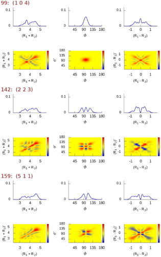
Figure 4. Reduced-density-matrix plots of selected vibrational states of H${}_2{}^{16}$O, computed using symmetrised valence coordinates. Plots corresponding to the diagonal ${\mathrm{\Gamma }}_1^{\mathrm{D}}$ (first row for each state) as well as the full ${\mathrm{\Gamma }}_1$ (second row for each state) reduced-density-matrix elements are shown. The radial coordinates are in bohr, the angular coordinate is in degrees. The ${\mathrm{\Gamma }}_1$ density scales from negative (blue) to positive (red) values through zero (yellow) (colours only available online).

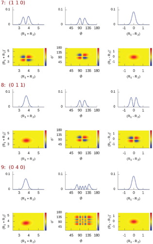
Figure 5. RDM plots of selected vibrational states of H${}_2{}^{16}$O, computed using symmetrised valence coordinates. Plots corresponding to the diagonal ${\mathrm{\Gamma }}_1^{\mathrm{D}}$ (first row for each state) as well as the full ${\mathrm{\Gamma }}_1$ (second row for each state) density matrix elements are shown. The radial coordinates are in bohr, the angular coordinate is in degrees. The ${\mathrm{\Gamma }}_1$ density scales from negative (blue) to positive (red) values through zero (yellow) (colours only available online).

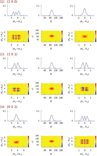
Figure 6. RDM plots of selected vibrational states of H${}_2{}^{16}$O, computed using symmetrised valence coordinates. Plots corresponding to the diagonal ${\mathrm{\Gamma }}_1^{\mathrm{D}}$ (first row of each state) as well as the full ${\mathrm{\Gamma }}_1$ (second row of each state) density matrix elements are shown. The radial coordinates are in bohr, the angular one is in degrees. The ${\mathrm{\Gamma }}_1$ density scales from negative (blue) to positive (red) values through zero (yellow) (colours only available online).

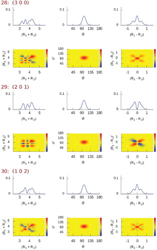
Figure 7. ${\mathrm{\Gamma }}_1^{\mathrm{D}}$ (first row of each state) and full ${\mathrm{\Gamma }}_1$ (second row of each state) reduced-density-matrix plots of selected vibrational states of H${}_2^{16}$O, computed using symmetrised valence coordinates. The radial coordinates are in bohr, the angular one is in degrees. The ${\mathrm{\Gamma }}_1$ density scales from negative (blue) to positive (red) values through zero (yellow) (colours only available online).

Almost all of the state assignments our semi-automatic scheme provided match nicely the assignments suggested in Ref. [20]. In cases of disagreement, the discrepancy is mostly a swap of neighbouring states, which may even be caused by using different potentials in the two studies. Successful assignment of higher vibrational states seems still possible, but it may require further improvement of the method or a careful visual inspection of the RDM plots. It is, however, not very clear until a further large number of studies is executed how far one can go with this approach based on modal density-structure similarities and the assumption of weakly interacting vibrational modes.

In Figures 2 and 3 we show plots of the diagonal densities for a few eigenstates. In states #7 $\left(110\right)$ and #8 $\left(011\right)$, respectively, one can see how the symmetric ($a_1$) and the antisymmetric ($b_2$) stretching-mode densities appear by means of the simple valence coordinates $R_1$ and $R_2$. States #12 $\left(200\right)$, #13 $\left(101\right)$, and #14 $\left(002\right)$ (Figure 2) represent the simplest stretching combinations, these states are remarkably easy to assign just by inspecting their density shapes. However, the more involved the stretching-mode combinations, the more complicated the density structure and the less obvious the visual assignment become, as noticable in Figure 3, especially for states #30 $\left(102\right)$, #99 $\left(104\right)$, and #142 $\left(223\right)$. Fortunately, when such structures first appear, their assignment tends to be very logical and their further occurrence is mostly undoubtfully recognised by the overlap computations.

Figures 4 and 5 provide beautiful examples of well-resolved nodal structures by the ${\mathrm{\Gamma }}_1$ matrices in the symmetrised valence coordinates for some of the low-lying states. However, the use of symmetrised coordinates during the semi-automatic assignment process proved to be significantly less successful than the use of simple internal coordinates. Even though the lowest 125 states could be straightforwardly assigned, almost automatically, after that the assignment became challenging with many ambiguous and unclear density structures. As examples of such difficult cases, in Figure 6 one can see that states #28 $\left(300\right)$ and #30 $\left(102\right)$ exhibit almost indistinguishable diagonal densities and just from their shapes it is hard to guess the correct assignment (this situation is in contrast to the clear ${\mathrm{\Gamma }}_2^{\mathrm{D}}(R_1,R_2)$ plots of Figure 3 based on simple valence coordinates). Only the full ${\mathrm{\Gamma }}_1$ density plots are a bit more helpful by better pronouncing the nodal structure in the $(R_1+R_2)$ and $(R_1-R_2)$ coordinates. Therefore, we decided to compare the ${\mathrm{\Gamma }}_1$ matrices rather than only their diagonals for the states described by the symmetrised valence coordinates. Assignment of the higher combination states in Figure 7 was substantially more difficult in the symmetrised than in the simple valence coordinates and in some cases intuition had to be used as the decision-making factor. All in all we managed to assign only about 180 states for reduced-density plots based on symmetrised valence coordinates. These problems may at least partly be due to the switch from normal- to a local-mode behaviour as the excitation increases.

6. Conclusions

In a previous study [25] we suggested using the diagonal elements of the one- and two-mode reduced-density matrices (RDM), corresponding to variationally computed wave functions, for the assignment of vibrational states. The main advantage of using RDMs over plotting wave functions is the compact representation of the information content and the higher number of assigned states that can be obtained, preferentially, semi-automatically. When densities are used, the nodal structure is represented by kinks in the density, with no direct observation of the sign changes characterising wave functions. This is, however, not a significant hindrance, the visual-only RDM-based assignment employing density kinks proved to be successful for the vinyl radical, whose vibrational energy-level structure is determined by a large-amplitude tunnelling motion [25]. During the present work the concept of using RDMs for the assignment of vibrational states was further investigated for the H${}_2{}^{16}$O test system, a semi-automatic assignment procedure was developed, and the possibility of directly observing the sign changes characterising wave-function nodes was explored.

The key idea behind the utility of RDMs is that the density of a mode excited by a given number of quanta tends to be very regular for most vibrational states. Hence the assignment procedure is tremendously helped by comparing density shapes via overlap computations.

The semi-automatic assignment procedure developed is based on ${\mathrm{\Gamma }}_1^{\mathrm{D}}$ and ${\mathrm{\Gamma }}_2^{\mathrm{D}}$ densities, overlap computations, a trivial excitation aufbau principle mechanism (preventing obvious misassignments), and a simple energy estimator. Together with the visual assessment of the densities in some cases, the proposed semi-automatic method allowed the successful assignment of 244 vibrational states of H${}_2{}^{16}$O (reaching over 24,900 cm⁻¹). In the case of H${}_2{}^{16}$O, it is advantageous to use simple valence coordinates for the computation of the densities.

By plotting a complete ${\mathrm{\Gamma }}_1$ matrix (not only the diagonal elements), one can observe the sign alternations characterising wave-function nodes; therefore, the visual node counting can be confirmed in cases when it is not clear whether a kink emerges due to a node or it is just a ‘density irregularity’.

For the RDM-based assignment we suggest to use an internal coordinate system whereby each coordinate represents well a single vibrational mode. This way the use of the ${\mathrm{\Gamma }}_2^{\mathrm{D}}$ matrices could be almost completely eliminated in favour of the ${\mathrm{\Gamma }}_1^{\mathrm{D}}$ plots and the nodal structure could be directly read from the ${\mathrm{\Gamma }}_1$ matrices. A semi-automatic assignment procedure developed used this approach, as well, whereby the full ${\mathrm{\Gamma }}_1$ matrices instead of the ${\mathrm{\Gamma }}_1^{\mathrm{D}}$ elements were compared for better state resolution. This way we were able to assign about 180 vibrational states of water (over 0–22,000  cm⁻¹) based on the use of symmetrised valence coordinates.

Naturally, lot more states could be assigned by the proposed method(s) if it was acceptable to leave out certain states from the assignment procedure. Further studies are needed to establish how high in energy one can go with the proposed approach based on modal density structure comparisons and the assumption of weakly interacting vibrational modes. We suggest using an internal coordinate system for which the diagonal or full ${\mathrm{\Gamma }}_1$ and the diagonal ${\mathrm{\Gamma }}_2^{\mathrm{D}}$ matrices provide a sufficiently simple vibrational mode representation. These quantities can easily be plotted for ‘on-the-fly’ visual assessment and they require only negligible storage capacity. For larger molecules, one might wonder about the use of higher-rank RDM for visual inspection via appropriate two-dimensional projections. Unfortunately, the computational and storage demands grow substantially as the rank increases.

Disclosure statement

No potential conflict of interest was reported by the authors.

Additional information

Funding

The authors gratefully acknowledge the financial support they received from NKFIH [grant number K119658].

References

- A.G. Császár, C. Fábri, T. Szidarovszky, E. Mátyus, T. Furtenbacher and G. Czakó, Phys. Chem. Chem. Phys. 13, 1085 (2012). doi: 10.1039/C1CP21830A
- C. Eckart, Phys. Rev. 47, 552 (1935). doi: 10.1103/PhysRev.47.552
- J.K.G. Watson, Mol. Phys. 15, 479 (1968). doi: 10.1080/00268976800101381
- J.K.G. Watson, Mol. Phys. 19, 465 (1970). doi: 10.1080/00268977000101491
- H. Wei and T. Carrington, J. Chem. Phys. 101, 1343 (1994). doi: 10.1063/1.467827
- C. Fábri, M. Quack and A.G. Császár, J. Chem. Phys. 147, 134101 (2017). doi: 10.1063/1.4990297
- S.N. Yurchenko, A. Yachmenev and R.I. Ovsyannikov, J. Chem. Theory Comput. 13, 4368 (2017). doi: 10.1021/acs.jctc.7b00506
- P.B. Changala, “NITROGEN, Numerical and Iterative Techniques for Rovibronic Energies with General Internal Coordinates,” (2018). http://www.colorado.edu/nitrogen.
- M. Joyeux, S.C. Farantos and R. Schinke, J. Phys. Chem. A 106, 5407–5421 (2002). doi: 10.1021/jp0131065
- H.W. Kroto, Molecular Rotation Spectra (Dover, New York, 1992).
- E.B. Wilson Jr., J.C. Decius and P.C. Cross, Molecular Vibrations (McGraw-Hill, New York, 1955).
- J.W. Ellis, Phys. Rev. 33, 27 (1929). doi: 10.1103/PhysRev.33.27
- P. Jensen, Mol. Phys. 98, 1253 (2010). doi: 10.1080/002689700413532
- J. Tennyson, P.F. Bernath, L.R. Brown, A. Campargue, M.R. Carleer, A.G. Császár, R.R. Gamache, J.T. Hodges, A. Jenouvrier, O.V. Naumenko, O.L. Polyansky, L.S. Rothman, R.A. Toth, A.C. Vandaele, N.F. Zobov, L. Daumont, A.Z. Fazliev, T. Furtenbacher, I.F. Gordon, S.N. Mikhailenko and S.V. Shirin, J. Quant. Spectrosc. Radiat. Transf. 110, 573 (2009). doi: 10.1016/j.jqsrt.2009.02.014
- J. Tennyson, P.F. Bernath, L.R. Brown, A. Campargue, A.G. Császár, L. Daumont, R.R. Gamache, J.T. Hodges, O.V. Naumenko, O.L. Polyansky, L.S. Rothman, A.C. Vandaele, N.F. Zobov, A.R. Al Derzi, C. Fábri, A.Z. Fazliev, T. Furtenbacher, I.E. Gordon, L. Lodi and I.I. Mizus, J. Quant. Spectrosc. Rad. Transf. 117, 29 (2013). doi: 10.1016/j.jqsrt.2012.10.002
- E. Mátyus, C. Fábri, T. Szidarovszky, G. Czakó, W.D. Allen and A.G. Császár, J. Chem. Phys. 133, 034113 (2010). doi: 10.1063/1.3451075
- E. Mátyus, G. Czakó and A.G. Császár, J. Chem. Phys. 130, 134112 (2009). doi: 10.1063/1.3076742
- C. Fábri, E. Mátyus and A.G. Császár, J. Chem. Phys. 134, 074105 (2011). doi: 10.1063/1.3533950
- C. Fábri, E. Mátyus and A.G. Császár, Spectrochim. Acta A 119, 84 (2014). doi: 10.1016/j.saa.2013.03.090
- A.G. Császár, E. Mátyus, T. Szidarovszky, L. Lodi, N.F. Zobov, S.V. Shirin, O.L. Polyansky and J. Tennyson, J. Quant. Spectrosc. Radiat. Transfer 111, 1043 (2010). doi: 10.1016/j.jqsrt.2010.02.009
- D.A. Sadovskii, N.G. Fulton, J.R. Henderson, J. Tennyson and B.I. Zhilinskii, J. Chem. Phys. 99, 906 (1993). doi: 10.1063/1.465355
- J. Sarka and A.G. Császár, J. Chem. Phys. 144, 154309 (2016). doi: 10.1063/1.4946808
- M. Gruebele, J. Chem. Phys. 104, 2453 (1996). doi: 10.1063/1.470940
- H.-G. Yu, H. Song and M. Yang, J. Chem. Phys. 146, 224307 (2017).
- J. Šmydke, C. Fábri, J. Sarka and A. Császár, Phys. Chem. Chem. Phys. (2018). http://dx.doi.org/10.1039/C8CP04672G.
- E.F. Valeev, W.D. Allen, H. F. Schaefer III and A.G. Császár, J. Chem. Phys. 114, 2875 (2001). doi: 10.1063/1.1346576
- M.S. Child, T. Weston and J. Tennyson, Mol. Phys. 96, 371 (1999). doi: 10.1080/00268979909482971
- Z. Bacic and J.C. Light, Annu. Rev. Phys. Chem. 40, 469 (1989). doi: 10.1146/annurev.pc.40.100189.002345
- J.C. Light and T. Carrington, “Discrete-Variable Representations and Their Utilization,” in Advances in Chemical Physics (John Wiley & Sons, Inc., 2007), pp. 263–310. 10.1002/9780470141731.ch4.
- C. Lanczos, J. Res. Natl. Bur. Stand. 45, 255 (1950). doi: 10.6028/jres.045.026
- H. Partridge and D.W. Schwenke, J. Chem. Phys. 106, 4618 (1997). doi: 10.1063/1.473987
- M. Carleer, A. Jenouvrier, A.-C. Vandaele, P.F. Bernath, M.F. Marienne, R. Colin, N.F. Zobov, O.L. Polyansky, J. Tennyson and V.A. Savin, J. Chem. Phys. 111, 2444 (1999). doi: 10.1063/1.479859