Improving the accuracy of computing chemical potentials in CFCMC simulations

ABSTRACT

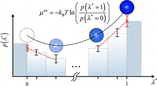
The CFCMC simulation methodology considers an expanded ensemble to solve the problem of low insertion/deletion acceptance probabilities in open ensembles. It allows for a direct calculation of the chemical potential by binning of the coupling parameter λ and using the probabilities $p(\lambda =0)$ and $p(\lambda =1)$, which require extrapolation. Here, we show that this extrapolation leads to systematic errors when the distribution $p\left(\lambda \right)$ is steep. We propose an alternative binning scheme which improves the accuracy of computed chemical potentials. We also investigate the use of multiple fractional molecules needed in simulations of multiple components, and show that these fractional molecules are very weakly correlated and that calculations of chemical potentials are not affected. The statistics of Boltzmann averages in systems with multiple fractional molecules is shown to be poor. Good agreement is found between CFCMC averages (uncorrected for the bias) and Boltzmann averages when the number of fractional molecules is less than 1% of the total number of all molecules. We found that, in dense systems, biased averages have a smaller uncertainty compared to Boltzmann averages.

GRAPHICAL ABSTRACT

KEYWORDS:

• Molecular simulation
• chemical potentials
• continuous fractional component Monte Carlo
• expanded ensembles

1. Introduction

Knowledge on Vapor–Liquid Equilibrium (VLE)/reaction equilibria and chemical potentials is important for process design and modelling [1–3]. The past decades, force field-based molecular simulation has been developed as an attractive alternative for experiments, to accurately describe the behaviour of matter, and to obtain reliable thermodynamic and transport properties [4–10]. Force field-based molecular modelling is used extensively for studying phase equilibria of pure and multicomponent systems [11–15], describing the behaviour of guest molecules inside porous media [16–19], and reaction equilibria [19–25] etc. In his pioneering work in 1987, Panagiotopoulos introduced the Gibbs Ensemble (GE) to directly determine the phase coexistence properties using Monte Carlo (MC) simulations [26–28]. In the GE, sufficient molecular exchanges between the phases leads to equal chemical potentials (which are directly related to activity/fugacity coefficients). The chemical potentials of components in each phase can be obtained from GE simulations using a variation of Widom's Test Particle Insertion (WTPI) method [29], taking into account the density fluctuations of each phase [2]. Computation of the chemical potential in the GE is an independent and important check on chemical equilibrium [1], and it can also be used to detect programming errors and errors in the implementation of the simulation technique.

The GE is widely used for VLE calculations [1,28]. It is a simple and fast method to obtain relatively accurate critical properties for most systems, using relatively small system sizes [15,30]. For accurate VLE calculations in the GE, one relies on sufficient molecule exchanges between the phases. A major drawback is that the acceptance probabilities of molecule insertions/deletions are very low in dense systems or systems with strong/directional intermolecular interactions, e.g. for water at ambient conditions [3,31]. Another drawback is that computing the excess chemical potential in the GE using insertion/deletion methods [29,32–35] suffers severely from molecule overlaps or random cavity formation. Methods based on the WTPI method are known to perform poorly for high density systems, even when combined with CBMC or related methods [1,31,36,37]. Due to the difficulties associated with free energy calculations and molecule exchanges in systems with high densities, other methods are required to facilitate phase equilibrium calculations in MC simulations.

To solve the sampling problems of the WTPI method, alternative methods are developed to obtain chemical potentials by combining particle insertions and removals [38,39], or by gradual insertions/deletions in multiple MC steps such that the surrounding molecules can adjust to the molecule that is inserted or deleted [37,40,41]. In the past decades, the idea of gradual insertion/deletion was used for different systems, see the works of Mon et al. [40], Squire et al. [42], Mruzik et al. [43] and de Pablo from the 90s [44]. A few years ago, the Continuous Fractional Component Monte Carlo (CFCMC) technique was developed by Shi and Maginn [45,46], leading to efficient molecule exchanges in open ensembles. The main difference with other methods is that the gradual insertion of molecules is continuous, rather than in discrete stages [47,48]. The CFCMC method has been applied to the NPT/NVT ensemble [49], grand-canonical (GC) [50], Gibbs Ensembe (GE) [45,46,49,51] and the reaction ensemble (RxMC) [25,52]. In the CFCMC method, a fractional molecule with scaled interactions with the surroundings is added to the ensemble. A coupling parameter λ is introduced as an extended variable in an expanded ensemble, and trial moves are carried out to change the value of λ. The fractional molecule is distinguishable from the other ‘whole’, or normal molecules. The value $\lambda =0$ means that the fractional molecule does not interact with other molecules in the simulation box and acts as an ‘ideal gas’ molecule. The value $\lambda =1$ means that the fractional molecule is fully interacting with other molecules in the system, and thus acts as a ‘whole’ molecule. To further increase the efficiency of molecule exchanges, an additional biasing potential $W\left(\lambda \right)$ can be used to ensure that the sampled probability distribution of λ is flat [45,46,53,54]. The Lennard-Jones (LJ) interactions of the fractional molecule with the rest of the molecules is often scaled as follows [49,51,52,55]: (1) $\begin{array}{rl}{u}_{\mathrm{L}\mathrm{J}}\left(r,{\lambda }_{\mathrm{L}\mathrm{J}}\right)& ={\lambda }_{\mathrm{L}\mathrm{J}}4ϵ\left(\frac{1}{{\left[\frac{1}{2}{\left(1-{\lambda }_{\mathrm{L}\mathrm{J}}\right)}^2+{\left(\frac{r}{\sigma }\right)}^6\right]}^2}\right.\\ & \left.-\frac{1}{\left[\frac{1}{2}{\left(1-{\lambda }_{\mathrm{L}\mathrm{J}}\right)}^2+{\left(\frac{r}{\sigma }\right)}^6\right]}\right)\end{array}$(1) in which, σ and ε are the LJ parameters and r is the intermolecular distance between two interaction sites. In principle, other thermodynamic pathways are possible to scale the interactions of the LJ molecule between $\lambda =0$ and $\lambda =1$ [56–58]. The scaling of the electrostatic interactions are explained in Refs. [11,52,55]. In principle, the λ-space can be chosen discrete [47] or continuous [45,46,51]. If the λ-space is discrete, it is limited to a certain number of states between (and including) 0 and 1. To avoid high energy barriers for gradual insertions/removals, the number of these states has to be carefully chosen for each system. The main new element of the method by Shi and Maginn is that λ has been changed from a discrete parameter into a continuous parameter [45,46]. The advantages of having a continuous λ-space is that changes in λ (denoted by $\mathrm{\Delta }\lambda$) can be adjusted during the simulation to facilitate transfers between intermediate λ states. Since in CFCMC simulations, insertions/deletions are performed with fractional molecules, biasing of λ is used to improve molecule transfer efficiency [45,46,51,52]. Adaptive computation of the weight function $W\left(\lambda \right)$ is performed iteratively to obtain a flat distribution of λ [53,54]. This significantly improves the efficiency of CFCMC simulations. Using an optimum weight function in the simulations ensures smooth transitions between $\lambda =0$ and $\lambda =1$. In CFCMC simulations, ensemble averages of thermodynamic properties can be computed, either Boltzmann averages or biased averages (uncorrected for the bias introduced by the biasing potential $W\left(\lambda \right)$). The Boltzmann average of any observable X is obtained from [51,52]: (2) ${⟨X⟩}_{\mathrm{B}\mathrm{o}\mathrm{l}\mathrm{t}\mathrm{z}\mathrm{m}\mathrm{a}\mathrm{n}\mathrm{n}}=\frac{{⟨X\exp \left[-W\left(\lambda \right)\right]⟩}_{\mathrm{C}\mathrm{F}\mathrm{C}\mathit{N}\mathit{P}\mathit{T}}}{{⟨\exp \left[-W\left(\lambda \right)\right]⟩}_{\mathrm{C}\mathrm{F}\mathrm{C}\mathit{N}\mathit{P}\mathit{T}}}.$(2) Equation (2(2) ${⟨X⟩}_{\mathrm{B}\mathrm{o}\mathrm{l}\mathrm{t}\mathrm{z}\mathrm{m}\mathrm{a}\mathrm{n}\mathrm{n}}=\frac{{⟨X\exp \left[-W\left(\lambda \right)\right]⟩}_{\mathrm{C}\mathrm{F}\mathrm{C}\mathit{N}\mathit{P}\mathit{T}}}{{⟨\exp \left[-W\left(\lambda \right)\right]⟩}_{\mathrm{C}\mathrm{F}\mathrm{C}\mathit{N}\mathit{P}\mathit{T}}}.$(2) ) is used to transform the averages back to the CFCNPT ensemble [51,52]. Biased averages are obtained by taking the normal averages without correcting for the bias: (3) ${⟨X⟩}_{\mathrm{B}\mathrm{i}\mathrm{a}\mathrm{s}\mathrm{e}\mathrm{d}}=\frac{\sum _{i=1}^{N_{\mathrm{S}}}X}{N_{\mathrm{S}}},$(3) where $N_{\mathrm{S}}$ is the number of times X is sampled. The averages of Equation (3(3) ${⟨X⟩}_{\mathrm{B}\mathrm{i}\mathrm{a}\mathrm{s}\mathrm{e}\mathrm{d}}=\frac{\sum _{i=1}^{N_{\mathrm{S}}}X}{N_{\mathrm{S}}},$(3) ) may be considered as approximations for averages in the CFCNPT ensemble, which in turn are approximations for averages in the conventional NPT ensemble. As the CFCNPT and conventional NPT ensemble have a different number of degrees of freedom [1,49], ensemble averages in both ensembles are in principle different, but in practice these differences are small [51,52]. Based on the earlier work of Shi and Maginn [45,46], recent work of Vlugt and co-workers, combines CFCMC in open ensembles (GC, reaction ensemble, Gibbs ensemble) with free energy calculations, in which molecule transfers are facilitated by CFCMC [51,52]. In those CFCMC simulations, the excess chemical potential can be computed by sampling the Boltzmann probability distribution of the coupling parameter, $p\left(\lambda \right)$. The ratio between $p(\lambda =0)$ and $p(\lambda =1)$ is directly related to the free energy difference of inserting a full additional molecule [51,52]. For a continuous λ-space, in this method, it is not possible to directly sample $p(\lambda =0)$ and $p(\lambda =1)$. One could only perform extrapolation on the averages of the few first/last bins to estimate $p(\lambda =0)$ and $p(\lambda =1)$. Therefore, it is necessary to use a binning scheme to sample the distribution $p\left(\lambda \right)$. The excess chemical potential is related to the Boltzmann probability distribution of λ [49,51,52]: (4) ${\mu }^{\mathrm{e}\mathrm{x}}=-\frac{1}{\beta }\ln \left(\frac{p(\lambda \uparrow 1)}{p(\lambda \downarrow 0)}\right).$(4) Here $p(\lambda \uparrow 1)$ is the probability of $\lambda \in ⟨0,1⟩$ approaching 1 and $p(\lambda \downarrow 0)$ is the probability of λ approaching zero. Recently, free energy calculations using Equation (4(4) ${\mu }^{\mathrm{e}\mathrm{x}}=-\frac{1}{\beta }\ln \left(\frac{p(\lambda \uparrow 1)}{p(\lambda \downarrow 0)}\right).$(4) ) were applied to phase equilibria and reaction equilibria: computation of chemical potentials of coexisting gas and liquid phases of water, methanol, hydrogen sulfide and carbon dioxide between $T=220K$ and $T=375K$ [3], and computing the reaction equilibrium of the Haber-Bosch process for pressures between 100 bar to 1000 bar [52,59]. We also combined the recent CFCMC method with the idea of Frenkel, Ciccotti, and co-workers [60,61] to obtain partial derivatives of the chemical potential with respect to pressure and temperature in the expanded NPT ensemble. The method was also used to calculate the enthalpy of reaction of the Haber–Bosch process for pressures between 100 bar to 800 bar [49].

In our current version of the CFCMC method  [3,49,51,52,55], one relies on extrapolation to $\lambda \to 0$ and $\lambda \to 1$ to compute the excess chemical potential (Equation (4(4) ${\mu }^{\mathrm{e}\mathrm{x}}=-\frac{1}{\beta }\ln \left(\frac{p(\lambda \uparrow 1)}{p(\lambda \downarrow 0)}\right).$(4) )) which may affect the accuracy of the method. In Ref. [51] it was proposed that in practice linear extrapolation of $p\left(\lambda \right)$ is sufficient to calculate the excess chemical potential using Equation (4(4) ${\mu }^{\mathrm{e}\mathrm{x}}=-\frac{1}{\beta }\ln \left(\frac{p(\lambda \uparrow 1)}{p(\lambda \downarrow 0)}\right).$(4) ). A clear distinction needs to be made between ‘precise’ and ‘accurate’ computation of the excess chemical potential. The values for the computed excess chemical potential may be systematically wrong (inaccurate) with small error bars (precise). This leads to a false impression of precision while missing accuracy (large difference from the actual value). This sampling issue appears especially for systems in which the number of bins, $N_{\mathrm{b}}$, is insufficient to capture the steepness of distribution $p\left(\lambda \right)$, leading to inaccurate extrapolation results. One could increase $N_{\mathrm{b}}$ to improve the accuracy of the extrapolation, however this leads to poor sampling of $p\left(\lambda \right)$ (less statistics per bin) and therefore loss of precision of the extrapolation. Therefore, it is not a priori clear which value to select for $N_{\mathrm{b}}$ for different systems. In this work, we investigate how the accuracy of the extrapolation scheme changes with $N_{\mathrm{b}}$, and we develop a much more accurate scheme that allows a continuous coupling parameter $\lambda \in [0,1]$ without having to use extrapolation for chemical potential calculations. The new scheme allows sampling a continuous coupling parameter including the states $\lambda =0$ and $\lambda =1$. This means that the chemical potential is obtained independent of any extrapolation scheme since the states $\lambda =0$ and $\lambda =1$ are directly sampled. We will show that this significantly improves the accuracy of computed values of ${\mu }^{\mathrm{e}\mathrm{x}}$ for systems with strong intermolecular interactions. In principle, the intermediate λ states can be either continuous or discrete. Continuous and discrete intermediate stages for λ are both commonly used in expanded ensembles [45–47]. The advantage of having a continuous λ is that changes in λ can be adjusted to facilitate transfers between intermediate λ states. This eliminates the guesswork about how many intermediate stages are needed. When the number of intermediate stages is close to optimal, we do not expect much differences in the accuracy of the computed chemical potentials between continuous and discrete staging. The effect of $N_{\mathrm{b}}$ on the accuracy and precision of our new binning scheme is also investigated.

Simulations in the CFCMC ensemble with multiple fractional molecules may be used to study complex systems e.g. the multicomponent Gibbs ensemble [62], the reaction ensemble [49,52] and the reaction ensemble combined with phase equilibria [21,23,24]. It is not recommended to include more fractional molecules in the system than required. However, in many cases it is necessary to use multiple fractional molecules [52]. Therefore, it is important to understand how multiple fractional molecules influence computed properties. For dense systems or systems in which $N_{\mathrm{f}\mathrm{r}\mathrm{a}\mathrm{c}}$ fractional molecules are present, the multidimensional weight function $W({\lambda }_1,{\lambda }_2,\dots ,{\lambda }_{N_{\mathrm{f}\mathrm{r}\mathrm{a}\mathrm{c}}})$ becomes steeper with increasing $N_{\mathrm{f}\mathrm{r}\mathrm{a}\mathrm{c}}$. This results in difficulties when sampling Boltzmann averages (Equation (9(9) ${⟨X⟩}_{\mathrm{B}\mathrm{o}\mathrm{l}\mathrm{t}\mathrm{z}\mathrm{m}\mathrm{a}\mathrm{n}\mathrm{n}}=\frac{{⟨X\exp \left[-\sum _{i=1}^{N_{\mathrm{f}\mathrm{r}\mathrm{a}\mathrm{c}}}{W}_i\left({\lambda }_i\right)\right]⟩}_{\mathrm{C}\mathrm{F}\mathrm{C}\mathit{N}\mathit{P}\mathit{T}}}{{⟨\exp \left[-\sum _{i=1}^{N_{\mathrm{f}\mathrm{r}\mathrm{a}\mathrm{c}}}{W}_i\left({\lambda }_i\right)\right]⟩}_{\mathrm{C}\mathrm{F}\mathrm{C}\mathit{N}\mathit{P}\mathit{T}}}.$(9) )). In principle, $N_{\mathrm{f}\mathrm{r}\mathrm{a}\mathrm{c}}$ is the number of fractional molecule types in the simulation. This is important to consider when performing simulations in the reaction ensemble as fractional molecule types of reactants and reaction products are different [52]. For the rest of this work, all fractional types are considered the same, however the conclusions are transferable to the reaction ensemble [52]. Another drawback is the difficulty of computing the multidimensional weight function using an adaptive scheme such as the Wang–Landau algorithm [53,54]. To calculate the biasing function, a multidimensional histogram has to be filled until some flatness criterion is met, which can be difficult computationally. We find that splitting the multidimensional weight function into a sum of one-dimensional weight functions can improve the calculation of the biasing function $W\left(\lambda \right)$ and sampling of Boltzmann averages. To the best of our knowledge, the effect of having multiple fractional molecules on the statistics of Boltzmann averages and biasing in CFCMC simulations are not systematically investigated/reported in literature. In this work, three important points relevant to systems with multiple fractional molecules are investigated: (1) The correlation between λ's of different fractional molecules are investigated.  (2) Sampling of Boltzmann averages using Equation (2(2) ${⟨X⟩}_{\mathrm{B}\mathrm{o}\mathrm{l}\mathrm{t}\mathrm{z}\mathrm{m}\mathrm{a}\mathrm{n}\mathrm{n}}=\frac{{⟨X\exp \left[-W\left(\lambda \right)\right]⟩}_{\mathrm{C}\mathrm{F}\mathrm{C}\mathit{N}\mathit{P}\mathit{T}}}{{⟨\exp \left[-W\left(\lambda \right)\right]⟩}_{\mathrm{C}\mathrm{F}\mathrm{C}\mathit{N}\mathit{P}\mathit{T}}}.$(2) ) is numerically difficult if the weight function is large. Due to this, sampling of the biased averages, Equation (3(3) ${⟨X⟩}_{\mathrm{B}\mathrm{i}\mathrm{a}\mathrm{s}\mathrm{e}\mathrm{d}}=\frac{\sum _{i=1}^{N_{\mathrm{S}}}X}{N_{\mathrm{S}}},$(3) ), is an attractive alternative to Boltzmann averages in CFCMC simulations. Therefore, it is of interest to study the difference between the Boltzmann and biased averages for different systems. (3) The excess chemical potential is a thermodynamic property for any system state, independent of the number of the fractional molecules, $N_{\mathrm{f}\mathrm{r}\mathrm{a}\mathrm{c}}$. Therefore, it is important to check whether the value of the computed chemical potentials varies with $N_{\mathrm{f}\mathrm{r}\mathrm{a}\mathrm{c}}$.

This paper is organised as follows. In Section 2, a binning scheme is introduced as to directly sample the chemical potential of a component. For this scheme, a continuous coupling parameter ${\lambda }^{\ast }\left(\lambda \right)\in [0,1]$ is introduced by a linear transformation of λ. The expression for computing the excess chemical potential using this method is described. The mathematical framework for calculating correlations between multiple fractional molecules in a single CFCMC ensemble simulation is described. The theory on using biased averages instead of Boltzmann averages is also discussed in this section. The direct sampling of ${\lambda }^{\ast }\left(\lambda \right)=0$ and ${\lambda }^{\ast }\left(\lambda \right)=1$ is tested both for a 2-atom model system consisting of two LJ molecules and liquid water. Simulation details, force field parameters and the scaling of the intramolecular interactions are described in Section 3. Our simulation results are presented in Section 4. It is shown that the excess chemical potential can be obtained accurately only by using the values from the first and the last bins of the histogram of $p\left({\lambda }^{\ast }\right(\lambda \left)\right)$, independent of any extrapolation scheme. Correlations between different λ's in CFCMC simulations with multiple fractional molecules are investigated in Section 4. The systems selected for this study are LJ colour mixtures with different numbers of fractional molecules, and equimolar mixtures of water and methanol with a fractional molecule of each molecule type. It is shown that fractional molecules are very weakly correlated (essentially uncorrelated) independent of the biasing. The differences associated with using Boltzmann averages and biased averages in CFCMC simulations with multiple fractional molecules are compared to Boltzmann averages obtained from the conventional NPT ensemble. The ensemble averages obtained from conventional NPT simulations are considered as a reference. The results show that in systems in which the ratio between the fractional molecules and the total number of molecules are below 1%, Boltzmann and biased averages for density, volume and energy are very similar. However, the error bars associated with Boltzmann averages can be an order of magnitude larger compared to biased averages, especially for dense systems. Our conclusions are summarised in Section 5.

2. Theory and computational methods

In our previous work, a continuous coupling parameter $\lambda \in ⟨0,1⟩$, corresponding to each fractional molecule type was used in the partition function [3,11,49,51,52,63], and atomistic/molecular interactions were scaled with λ (e.g. according to Equation (1(1) $\begin{array}{rl}{u}_{\mathrm{L}\mathrm{J}}\left(r,{\lambda }_{\mathrm{L}\mathrm{J}}\right)& ={\lambda }_{\mathrm{L}\mathrm{J}}4ϵ\left(\frac{1}{{\left[\frac{1}{2}{\left(1-{\lambda }_{\mathrm{L}\mathrm{J}}\right)}^2+{\left(\frac{r}{\sigma }\right)}^6\right]}^2}\right.\\ & \left.-\frac{1}{\left[\frac{1}{2}{\left(1-{\lambda }_{\mathrm{L}\mathrm{J}}\right)}^2+{\left(\frac{r}{\sigma }\right)}^6\right]}\right)\end{array}$(1) )). Therefore, it was not possible to directly sample the system states in which exactly $\lambda =0$ or $\lambda =1$. Here, we introduce a coupling parameter ${\lambda }^{\ast }\left(\lambda \right)\in [0,1]$ to calculate the atomistic/molecular interactions, including system states when the interactions of the fractional molecule are completely switched on or off. e.g. for LJ interactions, this means that λ in Equation (1(1) $\begin{array}{rl}{u}_{\mathrm{L}\mathrm{J}}\left(r,{\lambda }_{\mathrm{L}\mathrm{J}}\right)& ={\lambda }_{\mathrm{L}\mathrm{J}}4ϵ\left(\frac{1}{{\left[\frac{1}{2}{\left(1-{\lambda }_{\mathrm{L}\mathrm{J}}\right)}^2+{\left(\frac{r}{\sigma }\right)}^6\right]}^2}\right.\\ & \left.-\frac{1}{\left[\frac{1}{2}{\left(1-{\lambda }_{\mathrm{L}\mathrm{J}}\right)}^2+{\left(\frac{r}{\sigma }\right)}^6\right]}\right)\end{array}$(1) ) is replaced by ${\lambda }^{\ast }$, which is a function of λ. ${\lambda }^{\ast }\left(\lambda \right)$ is obtained from linear transformation of λ: (5) $\begin{array}{r}{\lambda }^{\ast }\left(\lambda \right)\equiv \left\{\begin{array}{ll}0,& \lambda <\frac{1}{N_{\mathrm{b}}}\\ \frac{N_{\mathrm{b}}\lambda -1}{N_{\mathrm{b}}-2},\frac{1}{N_{\mathrm{b}}}\le & \lambda \le \frac{N_{\mathrm{b}}-1}{N_{\mathrm{b}}}\\ 1,& \lambda >\frac{N_{\mathrm{b}}-1}{N_{\mathrm{b}}}\end{array}\right.\end{array}$(5) in which $N_{\mathrm{b}}$ is the number of the bins. It is important to note that the extended parameter in the partition function is still $\lambda \in ⟨0,1⟩$. Using the transformation of Equation (5(5) $\begin{array}{r}{\lambda }^{\ast }\left(\lambda \right)\equiv \left\{\begin{array}{ll}0,& \lambda <\frac{1}{N_{\mathrm{b}}}\\ \frac{N_{\mathrm{b}}\lambda -1}{N_{\mathrm{b}}-2},\frac{1}{N_{\mathrm{b}}}\le & \lambda \le \frac{N_{\mathrm{b}}-1}{N_{\mathrm{b}}}\\ 1,& \lambda >\frac{N_{\mathrm{b}}-1}{N_{\mathrm{b}}}\end{array}\right.\end{array}$(5) ), only the interactions of the fractional molecule are scaled with ${\lambda }^{\ast }\left(\lambda \right)\in [0,1]$ in an extra step. Note that the electrostatic interactions of the fractional molecule can also be scaled in a similar manner using the transformation of Equation (5(5) $\begin{array}{r}{\lambda }^{\ast }\left(\lambda \right)\equiv \left\{\begin{array}{ll}0,& \lambda <\frac{1}{N_{\mathrm{b}}}\\ \frac{N_{\mathrm{b}}\lambda -1}{N_{\mathrm{b}}-2},\frac{1}{N_{\mathrm{b}}}\le & \lambda \le \frac{N_{\mathrm{b}}-1}{N_{\mathrm{b}}}\\ 1,& \lambda >\frac{N_{\mathrm{b}}-1}{N_{\mathrm{b}}}\end{array}\right.\end{array}$(5) ). It follows directly from Equation (5(5) $\begin{array}{r}{\lambda }^{\ast }\left(\lambda \right)\equiv \left\{\begin{array}{ll}0,& \lambda <\frac{1}{N_{\mathrm{b}}}\\ \frac{N_{\mathrm{b}}\lambda -1}{N_{\mathrm{b}}-2},\frac{1}{N_{\mathrm{b}}}\le & \lambda \le \frac{N_{\mathrm{b}}-1}{N_{\mathrm{b}}}\\ 1,& \lambda >\frac{N_{\mathrm{b}}-1}{N_{\mathrm{b}}}\end{array}\right.\end{array}$(5) ) that ${\lambda }^{\ast }\left(\lambda \right)$ is a continuous function at $\lambda =\frac{1}{N_{\mathrm{b}}}$ and $\lambda =\frac{N_{\mathrm{b}}-1}{N_{\mathrm{b}}}$. Scaling the interactions of the fractional molecule using ${\lambda }^{\ast }\left(\lambda \right)$ means that there are now two bins in λ space where interactions are completely switched on or off. Therefore, one can directly sample the probability of ${\lambda }^{\ast }\left(\lambda \right)=0$ in the first bin, and the probability of ${\lambda }^{\ast }\left(\lambda \right)=1$ in the last bin. The linear transformation of Equation (5(5) $\begin{array}{r}{\lambda }^{\ast }\left(\lambda \right)\equiv \left\{\begin{array}{ll}0,& \lambda <\frac{1}{N_{\mathrm{b}}}\\ \frac{N_{\mathrm{b}}\lambda -1}{N_{\mathrm{b}}-2},\frac{1}{N_{\mathrm{b}}}\le & \lambda \le \frac{N_{\mathrm{b}}-1}{N_{\mathrm{b}}}\\ 1,& \lambda >\frac{N_{\mathrm{b}}-1}{N_{\mathrm{b}}}\end{array}\right.\end{array}$(5) ) is illustrated in Figure 1 for $p\left(\lambda \right)$ and $p\left({\lambda }^{\ast }\right(\lambda \left)\right)$. The inset of this figure shows the function ${\lambda }^{\ast }\left(\lambda \right)$. 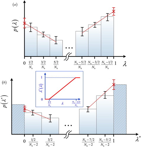As shown in Figure 1(a), $p\left(\lambda \right)$ is constructed by sampling the probability of λ where the λ space is binned at equal distances; $[\frac{1}{2},\frac{3}{2},\frac{5}{2},\dots ,N_{\mathrm{b}}-\frac{5}{2},N_{\mathrm{b}}-\frac{3}{2},N_{\mathrm{b}}-\frac{1}{2}]$ in units of $\frac{1}{N_{\mathrm{b}}}$. The width of each bin, $\mathrm{\Delta }\lambda$, equals $\frac{1}{N_{\mathrm{b}}}$ and value of λ assigned to each bin equals the middle of the bin, i.e. $\frac{i-1/2}{N_{\mathrm{b}}}$. Therefore, the value of λ in the first and last bins correspond to $\lambda =\frac{1}{2N_{\mathrm{b}}}$ and $\lambda =\frac{N_{\mathrm{b}}-1/2}{N_{\mathrm{b}}}$, respectively, and not to 0 or 1. To calculate ${\mu }^{\mathrm{e}\mathrm{x}}$ (Equation (4(4) ${\mu }^{\mathrm{e}\mathrm{x}}=-\frac{1}{\beta }\ln \left(\frac{p(\lambda \uparrow 1)}{p(\lambda \downarrow 0)}\right).$(4) )) from $p\left(\lambda \right)$ instead of $p\left({\lambda }^{\ast }\right(\lambda \left)\right)$, one needs to perform a linear extrapolation on the first/last few points of $p\left(\lambda \right)$ [51]. The distribution $p\left({\lambda }^{\ast }\right(\lambda \left)\right)$ can be directly reconstructed from $p\left(\lambda \right)$ in a single step using Equation (5(5) $\begin{array}{r}{\lambda }^{\ast }\left(\lambda \right)\equiv \left\{\begin{array}{ll}0,& \lambda <\frac{1}{N_{\mathrm{b}}}\\ \frac{N_{\mathrm{b}}\lambda -1}{N_{\mathrm{b}}-2},\frac{1}{N_{\mathrm{b}}}\le & \lambda \le \frac{N_{\mathrm{b}}-1}{N_{\mathrm{b}}}\\ 1,& \lambda >\frac{N_{\mathrm{b}}-1}{N_{\mathrm{b}}}\end{array}\right.\end{array}$(5) ). As shown in Figure 1(b), $p\left({\lambda }^{\ast }\right)$ is constructed using bins with the values of $[0,\frac{1}{2},\frac{3}{2},\dots ,N_{\mathrm{b}}-\frac{7}{2},N_{\mathrm{b}}-\frac{5}{2},1]$ in units of $\frac{1}{N_{\mathrm{b}}-2}$. This grid is continuous but non-equidistant. Using the new binning scheme, ${\mu }^{\mathrm{e}\mathrm{x}}$ can be obtained directly using the probabilities of the first and the last bin, as shown in Figure 1(b): (6) ${\mu }^{\mathrm{e}\mathrm{x}}=-\frac{1}{\beta }\ln \left(\frac{p({\lambda }^{\ast }\left(\lambda \right)=1)}{p({\lambda }^{\ast }\left(\lambda \right)=0)}\right).$(6) In principle one could directly sample $p(\lambda =0)$ and $p(\lambda =1)$ without any biasing (and hence no binning is required). However, it is well-known that not applying a biasing function $W\left(\lambda \right)$ significantly reduces the efficiency of the simulation [51,52]. In this work, we compare the differences between extrapolation, and direct sampling for calculating the chemical potential for different systems.

Figure 1. Linear transformation of the scaling parameter from λ (subfigure a) to ${\lambda }^{\ast }$ (subfigure b). Based on the transformation of Equation (5(5) $\begin{array}{r}{\lambda }^{\ast }\left(\lambda \right)\equiv \left\{\begin{array}{ll}0,& \lambda <\frac{1}{N_{\mathrm{b}}}\\ \frac{N_{\mathrm{b}}\lambda -1}{N_{\mathrm{b}}-2},\frac{1}{N_{\mathrm{b}}}\le & \lambda \le \frac{N_{\mathrm{b}}-1}{N_{\mathrm{b}}}\\ 1,& \lambda >\frac{N_{\mathrm{b}}-1}{N_{\mathrm{b}}}\end{array}\right.\end{array}$(5) ), the value ${\lambda }^{\ast }\left(\lambda \right)$ is set to zero for the first bin of $p\left(\lambda \right)$, and the value ${\lambda }^{\ast }\left(\lambda \right)$ equals one for the last bin. When the interaction parameter ${\lambda }^{\ast }\left(\lambda \right)=0$, the fractional molecule behaves as an ideal gas, and when ${\lambda }^{\ast }\left(\lambda \right)=1$, the fractional molecule behaves exactly as a whole molecule. The inset shows how ${\lambda }^{\ast }$ depends on λ (Equation (5(5) $\begin{array}{r}{\lambda }^{\ast }\left(\lambda \right)\equiv \left\{\begin{array}{ll}0,& \lambda <\frac{1}{N_{\mathrm{b}}}\\ \frac{N_{\mathrm{b}}\lambda -1}{N_{\mathrm{b}}-2},\frac{1}{N_{\mathrm{b}}}\le & \lambda \le \frac{N_{\mathrm{b}}-1}{N_{\mathrm{b}}}\\ 1,& \lambda >\frac{N_{\mathrm{b}}-1}{N_{\mathrm{b}}}\end{array}\right.\end{array}$(5) )).

The linear transformation of λ (Equation (5(5) $\begin{array}{r}{\lambda }^{\ast }\left(\lambda \right)\equiv \left\{\begin{array}{ll}0,& \lambda <\frac{1}{N_{\mathrm{b}}}\\ \frac{N_{\mathrm{b}}\lambda -1}{N_{\mathrm{b}}-2},\frac{1}{N_{\mathrm{b}}}\le & \lambda \le \frac{N_{\mathrm{b}}-1}{N_{\mathrm{b}}}\\ 1,& \lambda >\frac{N_{\mathrm{b}}-1}{N_{\mathrm{b}}}\end{array}\right.\end{array}$(5) )) can be easily implemented in the original CFCMC algorithm. For instance, the partition function of a mixture of S different monoatomic components in the NPT ensemble expanded with a fractional molecule equals [49] (7) $\begin{array}{rl}{Q}_{\mathrm{C}\mathrm{F}\mathrm{C}\mathit{N}\mathit{P}\mathit{T}}& =\beta P\left[\prod _{i=1}^S\frac{1}{{\mathrm{\Lambda }}_i^{3N_i}{N}_i!}\right]\\ & \times \frac{1}{{\mathrm{\Lambda }}^3}{\int }_0^1\mathrm{d}\lambda \int \mathrm{d}V{V}^{N+1}\exp \left[-\beta PV\right]\\ & \times \int \mathrm{d}{s}^N\exp [-\beta U(s^N,V\left)\right]\\ & \times \int \mathrm{d}{s}_{\mathrm{f}\mathrm{r}\mathrm{a}\mathrm{c}}^{\mathrm{A}}\exp [-\beta U_{\mathrm{f}\mathrm{r}\mathrm{a}\mathrm{c}}^{\mathrm{A}}(s_{\mathrm{f}\mathrm{r}\mathrm{a}\mathrm{c}}^{\mathrm{A}},s^N,{\lambda }^{\ast }\left(\lambda \right),V\left)\right]\end{array}$(7) in which N is the total number of whole molecules which are distinguishable from the fractional molecule, S is the number of components, ${\mathrm{\Lambda }}_i$ is the thermal wavelength of component i, Λ is the thermal wavelength of the fractional molecule, U is the total potential energy of the whole molecules and $U_{\mathrm{f}\mathrm{r}\mathrm{a}\mathrm{c}}^{\mathrm{A}}$ is the interaction potential of the fractional molecule with the surrounding molecules scaled with ${\lambda }^{\ast }\left(\lambda \right)$. No further changes are required for calculating the weight function $W\left(\lambda \right)$ and $p\left(\lambda \right)$ during the simulation [3,49,52]. Only at the end of the simulation, $p\left(\lambda \right)$ is transformed into $p\left({\lambda }^{\ast }\right(\lambda \left)\right)$ in a single step using Equation (5(5) $\begin{array}{r}{\lambda }^{\ast }\left(\lambda \right)\equiv \left\{\begin{array}{ll}0,& \lambda <\frac{1}{N_{\mathrm{b}}}\\ \frac{N_{\mathrm{b}}\lambda -1}{N_{\mathrm{b}}-2},\frac{1}{N_{\mathrm{b}}}\le & \lambda \le \frac{N_{\mathrm{b}}-1}{N_{\mathrm{b}}}\\ 1,& \lambda >\frac{N_{\mathrm{b}}-1}{N_{\mathrm{b}}}\end{array}\right.\end{array}$(5) ). Note that the CFCNPT ensemble is used here as an example to explain the method. The linear transformation of the λ can be implemented in open ensembles in a similar manner. The linear transformation of ${\lambda }^{\ast }\left(\lambda \right)$ has several advantages: (1) The first bin of $p\left(\lambda \right)$ corresponds to system states where the interaction potential is completely switched off (${\lambda }^{\ast }\left(\lambda \right)=0)$. At ${\lambda }^{\ast }\left(\lambda \right)=0$, reinsertions of the fractional molecule at a randomly selected position [49] are always accepted since the energy difference between the old and new configurations is zero. It is important to note that the fractional molecule is part of the ensemble partition function and is never deleted from the system even when ${\lambda }^{\ast }\left(\lambda \right)=0$. (2) The last bin of $p\left(\lambda \right)$, (${\lambda }^{\ast }\left(\lambda \right)=1$), corresponds to system states where the fractional molecule is interacting as a whole molecule. For ${\lambda }^{\ast }=1$, identity changes of the fractional molecule [49] with a whole molecule are always accepted as the energy difference between the old and new configurations is zero. In the identity change trial moves, the fractional molecule is changed into a whole molecule of the same type, and a randomly selected whole molecule of the same molecule type is changed into a fractional molecule, while keeping the value of λ, positions and orientations of the molecules unchanged [49,51,52]. The identity change trial move can also serve as an independent check of the correctness of the simulation code and the bookkeeping. Essentially, the transformation of Equation (5(5) $\begin{array}{r}{\lambda }^{\ast }\left(\lambda \right)\equiv \left\{\begin{array}{ll}0,& \lambda <\frac{1}{N_{\mathrm{b}}}\\ \frac{N_{\mathrm{b}}\lambda -1}{N_{\mathrm{b}}-2},\frac{1}{N_{\mathrm{b}}}\le & \lambda \le \frac{N_{\mathrm{b}}-1}{N_{\mathrm{b}}}\\ 1,& \lambda >\frac{N_{\mathrm{b}}-1}{N_{\mathrm{b}}}\end{array}\right.\end{array}$(5) ) allows rigorous sampling of the states $p\left({\lambda }^{\ast }\right(\lambda )=0)$ and $p\left({\lambda }^{\ast }\right(\lambda )=1)$ during the simulation without performing extrapolation. This method combines the benefits of free energy calculations in the CFCMC simulations with rigorous sampling of states in which ${\lambda }^{\ast }=0$ and ${\lambda }^{\ast }=1$ [47,49,51].

It is straightforward to extend the partition function of Equation (7(7) $\begin{array}{rl}{Q}_{\mathrm{C}\mathrm{F}\mathrm{C}\mathit{N}\mathit{P}\mathit{T}}& =\beta P\left[\prod _{i=1}^S\frac{1}{{\mathrm{\Lambda }}_i^{3N_i}{N}_i!}\right]\\ & \times \frac{1}{{\mathrm{\Lambda }}^3}{\int }_0^1\mathrm{d}\lambda \int \mathrm{d}V{V}^{N+1}\exp \left[-\beta PV\right]\\ & \times \int \mathrm{d}{s}^N\exp [-\beta U(s^N,V\left)\right]\\ & \times \int \mathrm{d}{s}_{\mathrm{f}\mathrm{r}\mathrm{a}\mathrm{c}}^{\mathrm{A}}\exp [-\beta U_{\mathrm{f}\mathrm{r}\mathrm{a}\mathrm{c}}^{\mathrm{A}}(s_{\mathrm{f}\mathrm{r}\mathrm{a}\mathrm{c}}^{\mathrm{A}},s^N,{\lambda }^{\ast }\left(\lambda \right),V\left)\right]\end{array}$(7) ) to systems with multiple fractional molecules [49]. In CFCMC simulations with multiple fractional molecules, the biasing function W is a multidimensional weight function [52] used to improve the efficiency of molecule insertions/removals and smooth transitions between $\lambda =0$ and $\lambda =1$ for every fractional molecule. However, calculating a multidimensional adaptive biasing function requires filling and flattening a multidimensional histogram during a random walk in $({\lambda }_1,{\lambda }_2,\dots )$ space, using a certain flatness criterion. Filling multidimensional histograms can be difficult with many fractional molecules in the system, e.g. using the Wang–Landau algorithm [53,54]. One could split the multidimensional biasing function into a series of one-dimensional biasing functions. For a system in which $N_{\mathrm{f}\mathrm{r}\mathrm{a}\mathrm{c}}$ fractional molecules are present, this leads to (8) $W\left({\lambda }_1,{\lambda }_2,\dots {\lambda }_{N_{\mathrm{f}\mathrm{r}\mathrm{a}\mathrm{c}}}\right)\approx \sum _{i=1}^{N_{\mathrm{f}\mathrm{r}\mathrm{a}\mathrm{c}}}{W}_i\left({\lambda }_i\right).$(8) Filling multiple independent one-dimensional histograms is computationally more straightforward than filling a single multidimensional histogram. The biasing is then calculated for each ${\lambda }_i$ independently. In Equation (8(8) $W\left({\lambda }_1,{\lambda }_2,\dots {\lambda }_{N_{\mathrm{f}\mathrm{r}\mathrm{a}\mathrm{c}}}\right)\approx \sum _{i=1}^{N_{\mathrm{f}\mathrm{r}\mathrm{a}\mathrm{c}}}{W}_i\left({\lambda }_i\right).$(8) ), it is assumed that the ${\lambda }_i$'s are independent coupling parameters. If there would be a strong correlation between λ's, the computed Boltzmann averages are still correct. However, the sampling of the distributions $p\left({\lambda }_i\right)$ may be very inefficient due to neglected correlations between λ's (Equation (8(8) $W\left({\lambda }_1,{\lambda }_2,\dots {\lambda }_{N_{\mathrm{f}\mathrm{r}\mathrm{a}\mathrm{c}}}\right)\approx \sum _{i=1}^{N_{\mathrm{f}\mathrm{r}\mathrm{a}\mathrm{c}}}{W}_i\left({\lambda }_i\right).$(8) )). By combining Equations (8(8) $W\left({\lambda }_1,{\lambda }_2,\dots {\lambda }_{N_{\mathrm{f}\mathrm{r}\mathrm{a}\mathrm{c}}}\right)\approx \sum _{i=1}^{N_{\mathrm{f}\mathrm{r}\mathrm{a}\mathrm{c}}}{W}_i\left({\lambda }_i\right).$(8) ) and (2(2) ${⟨X⟩}_{\mathrm{B}\mathrm{o}\mathrm{l}\mathrm{t}\mathrm{z}\mathrm{m}\mathrm{a}\mathrm{n}\mathrm{n}}=\frac{{⟨X\exp \left[-W\left(\lambda \right)\right]⟩}_{\mathrm{C}\mathrm{F}\mathrm{C}\mathit{N}\mathit{P}\mathit{T}}}{{⟨\exp \left[-W\left(\lambda \right)\right]⟩}_{\mathrm{C}\mathrm{F}\mathrm{C}\mathit{N}\mathit{P}\mathit{T}}}.$(2) ), the Boltzmann average of any observable X is obtained as follows (9) ${⟨X⟩}_{\mathrm{B}\mathrm{o}\mathrm{l}\mathrm{t}\mathrm{z}\mathrm{m}\mathrm{a}\mathrm{n}\mathrm{n}}=\frac{{⟨X\exp \left[-\sum _{i=1}^{N_{\mathrm{f}\mathrm{r}\mathrm{a}\mathrm{c}}}{W}_i\left({\lambda }_i\right)\right]⟩}_{\mathrm{C}\mathrm{F}\mathrm{C}\mathit{N}\mathit{P}\mathit{T}}}{{⟨\exp \left[-\sum _{i=1}^{N_{\mathrm{f}\mathrm{r}\mathrm{a}\mathrm{c}}}{W}_i\left({\lambda }_i\right)\right]⟩}_{\mathrm{C}\mathrm{F}\mathrm{C}\mathit{N}\mathit{P}\mathit{T}}}.$(9) In many systems with strong intermolecular interactions or with multiple fractional molecules, the weight function $\sum _{i=1}^{N_{\mathrm{f}\mathrm{r}\mathrm{a}\mathrm{c}}}{W}_i\left({\lambda }_i\right)$ is a large number, typically between ${10}^1$ and ${10}^2$ [49,55]. This means that the exponents in Equation (9(9) ${⟨X⟩}_{\mathrm{B}\mathrm{o}\mathrm{l}\mathrm{t}\mathrm{z}\mathrm{m}\mathrm{a}\mathrm{n}\mathrm{n}}=\frac{{⟨X\exp \left[-\sum _{i=1}^{N_{\mathrm{f}\mathrm{r}\mathrm{a}\mathrm{c}}}{W}_i\left({\lambda }_i\right)\right]⟩}_{\mathrm{C}\mathrm{F}\mathrm{C}\mathit{N}\mathit{P}\mathit{T}}}{{⟨\exp \left[-\sum _{i=1}^{N_{\mathrm{f}\mathrm{r}\mathrm{a}\mathrm{c}}}{W}_i\left({\lambda }_i\right)\right]⟩}_{\mathrm{C}\mathrm{F}\mathrm{C}\mathit{N}\mathit{P}\mathit{T}}}.$(9) ) are very small for such systems. This results in averaging over very small numbers, numerically close to zero, when sampling Boltzmann averages of Equation (9(9) ${⟨X⟩}_{\mathrm{B}\mathrm{o}\mathrm{l}\mathrm{t}\mathrm{z}\mathrm{m}\mathrm{a}\mathrm{n}\mathrm{n}}=\frac{{⟨X\exp \left[-\sum _{i=1}^{N_{\mathrm{f}\mathrm{r}\mathrm{a}\mathrm{c}}}{W}_i\left({\lambda }_i\right)\right]⟩}_{\mathrm{C}\mathrm{F}\mathrm{C}\mathit{N}\mathit{P}\mathit{T}}}{{⟨\exp \left[-\sum _{i=1}^{N_{\mathrm{f}\mathrm{r}\mathrm{a}\mathrm{c}}}{W}_i\left({\lambda }_i\right)\right]⟩}_{\mathrm{C}\mathrm{F}\mathrm{C}\mathit{N}\mathit{P}\mathit{T}}}.$(9) ). Therefore, taking Boltzmann averages for these systems may mostly lead to a $\frac{0}{0}$ numerical problem for ensemble averages like volume and energy. Except for excess chemical potentials, most ensemble averages hardly depend on the instantaneous values of λ's. In Refs. [51,63], it was shown that the presence of multiple fractional molecules hardly influences the thermodynamic properties of the system however, the statistics of the Boltzmann averages are affected. To avoid the $\frac{0}{0}$ sampling problem of the Boltzmann averages, a possible solution is to sample biased averages as shown in Equation (3(3) ${⟨X⟩}_{\mathrm{B}\mathrm{i}\mathrm{a}\mathrm{s}\mathrm{e}\mathrm{d}}=\frac{\sum _{i=1}^{N_{\mathrm{S}}}X}{N_{\mathrm{S}}},$(3) ). Here, we investigate how computed averages change with the number of fractional molecules. Preferably, one should use as few fractional molecules as possible in production runs. If no fractional molecules are required, it is recommended to use conventional ensembles instead of expanded ensembles.

It is not a priori clear whether fractional molecules are weakly or strongly correlated. The requirement for efficient splitting of the biasing, Equation (8(8) $W\left({\lambda }_1,{\lambda }_2,\dots {\lambda }_{N_{\mathrm{f}\mathrm{r}\mathrm{a}\mathrm{c}}}\right)\approx \sum _{i=1}^{N_{\mathrm{f}\mathrm{r}\mathrm{a}\mathrm{c}}}{W}_i\left({\lambda }_i\right).$(8) ), is that ${\lambda }_i$'s are independent. To validate this, we compute the pairwise correlation between different ${\lambda }_i$'s as a function of the number of fractional molecules in the system, while keeping the number of whole molecules constant. The pairwise correlation between two (randomly) selected ${\lambda }_i$'s in a simulation can be calculated by computing the correlation: (10) $\mathrm{Corr}\left({\lambda }_1,{\lambda }_2\right)=\frac{⟨{\lambda }_1{\lambda }_2⟩-⟨{\lambda }_1⟩⟨{\lambda }_2⟩}{\sqrt{\left[⟨{\lambda }_1^2⟩-{⟨{\lambda }_1⟩}^2\right]\left[⟨{\lambda }_2^2⟩-{⟨{\lambda }_2⟩}^2\right]}},$(10) where ${\lambda }_1$ and ${\lambda }_2$ are the instantaneous values of two randomly selected coupling parameters during the single simulation. Equation (10(10) $\mathrm{Corr}\left({\lambda }_1,{\lambda }_2\right)=\frac{⟨{\lambda }_1{\lambda }_2⟩-⟨{\lambda }_1⟩⟨{\lambda }_2⟩}{\sqrt{\left[⟨{\lambda }_1^2⟩-{⟨{\lambda }_1⟩}^2\right]\left[⟨{\lambda }_2^2⟩-{⟨{\lambda }_2⟩}^2\right]}},$(10) ) can be applied to systems with and without biasing. In addition, we investigate how the presence of multiple fractional components influences the computed values of ${\mu }^{\mathrm{e}\mathrm{x}}$ and other thermodynamic properties such as the average volume, density and energy.

3. Simulation details

As a proof of principle, the performance of the original binning scheme and the binning scheme of Equation (5(5) $\begin{array}{r}{\lambda }^{\ast }\left(\lambda \right)\equiv \left\{\begin{array}{ll}0,& \lambda <\frac{1}{N_{\mathrm{b}}}\\ \frac{N_{\mathrm{b}}\lambda -1}{N_{\mathrm{b}}-2},\frac{1}{N_{\mathrm{b}}}\le & \lambda \le \frac{N_{\mathrm{b}}-1}{N_{\mathrm{b}}}\\ 1,& \lambda >\frac{N_{\mathrm{b}}-1}{N_{\mathrm{b}}}\end{array}\right.\end{array}$(5) ) are compared for a 2-atom model system consisting of two LJ molecules in one-dimensional phase space. Here, reduced units are used, so $ϵ=1$ and $\sigma =1$. The 2-atom model system has two degrees of freedom, namely the interatomic distance r and λ. The partition function for this ensemble equals: (11) $Q=\frac{1}{L}{\int }_0^L\mathrm{d}r{\int }_0^1\mathrm{d}\lambda \exp [-\beta U(r,\lambda \left)\right],$(11) where we selected L=3, in units of σ, $\beta =1/T^{\ast }$ in reduced units, and $T^{\ast }$ is the reduced temperature. The interaction potential $U(r,\lambda )$ is a function of the distance $r\in [0,3]$ and $\lambda \in ⟨0,1⟩$, obtained from Equation (1(1) $\begin{array}{rl}{u}_{\mathrm{L}\mathrm{J}}\left(r,{\lambda }_{\mathrm{L}\mathrm{J}}\right)& ={\lambda }_{\mathrm{L}\mathrm{J}}4ϵ\left(\frac{1}{{\left[\frac{1}{2}{\left(1-{\lambda }_{\mathrm{L}\mathrm{J}}\right)}^2+{\left(\frac{r}{\sigma }\right)}^6\right]}^2}\right.\\ & \left.-\frac{1}{\left[\frac{1}{2}{\left(1-{\lambda }_{\mathrm{L}\mathrm{J}}\right)}^2+{\left(\frac{r}{\sigma }\right)}^6\right]}\right)\end{array}$(1) ). By performing long simulations, we can compute $p\left(\lambda \right)$ with brute-force sampling of λ and r. From the original binning scheme it follows that: (12) $p\left(\lambda \right)=\frac{\frac{1}{L}{\int }_0^L\mathrm{d}r{\int }_0^1\mathrm{d}{\lambda }^{\prime }\exp [-\beta U(r,{\lambda }^{\prime }\left)\right]\delta (\lambda -{\lambda }^{\prime })}{\frac{1}{L}{\int }_0^L\mathrm{d}r{\int }_0^1\mathrm{d}{\lambda }^{\prime }\exp [-\beta U(r,{\lambda }^{\prime }\left)\right]}.$(12) In the new binning scheme of Equation (5(5) $\begin{array}{r}{\lambda }^{\ast }\left(\lambda \right)\equiv \left\{\begin{array}{ll}0,& \lambda <\frac{1}{N_{\mathrm{b}}}\\ \frac{N_{\mathrm{b}}\lambda -1}{N_{\mathrm{b}}-2},\frac{1}{N_{\mathrm{b}}}\le & \lambda \le \frac{N_{\mathrm{b}}-1}{N_{\mathrm{b}}}\\ 1,& \lambda >\frac{N_{\mathrm{b}}-1}{N_{\mathrm{b}}}\end{array}\right.\end{array}$(5) ), the term $-\beta U(r,\lambda )$ is replaced by $-\beta U(r,{\lambda }^{\ast }(\lambda \left)\right)$ and after the simulation the distribution $p\left(\lambda \right)$ is converted to $p\left({\lambda }^{\ast }\right(\lambda \left)\right)$. Simulations are carried out at different temperatures between $T^{\ast }=0.005$ and $T^{\ast }=2$ in reduced units. For both binning schemes, the simulations at every temperature are repeated with different values of $N_{\mathrm{b}}$ ranging from 10 to 500. In each cycle, r and λ are randomly selected from uniform distributions, and the probability of λ is sampled using Equation (12(12) $p\left(\lambda \right)=\frac{\frac{1}{L}{\int }_0^L\mathrm{d}r{\int }_0^1\mathrm{d}{\lambda }^{\prime }\exp [-\beta U(r,{\lambda }^{\prime }\left)\right]\delta (\lambda -{\lambda }^{\prime })}{\frac{1}{L}{\int }_0^L\mathrm{d}r{\int }_0^1\mathrm{d}{\lambda }^{\prime }\exp [-\beta U(r,{\lambda }^{\prime }\left)\right]}.$(12) ). To compare the simulation results, a reference value of $p({\lambda }^{\ast }=1)$ is obtained from direct sampling of the last bin from simulations carried out 10 times longer. Since the value of the last bin is directly sampled, no systematic errors are present in this reference value. To obtain $p(\lambda \uparrow 1)$ in the original binning scheme, linear extrapolation is carried out using the last three points of the λ grid. $p\left({\lambda }^{\ast }\right(\lambda )=1)$ is obtained by directly sampling the last bin in the new binning scheme. For all the simulations, ${10}^8$ random states of $(r,\lambda )$ were generated to sample the probability of λ. To obtain the reference values for $p\left(\lambda \right)=1$, ${10}^9$ random states of $(r,\lambda )$ were generated.

Simulations of SPC/E [64] water and TraPPE methanol [65] are performed in the CFCNPT ensemble [49] at T=323.15 K and p=1 bar. Both the original and the new binning scheme are used to compute excess chemical potentials. To investigate the effect of binning on chemical potential calculations, simulations are performed with different values of the number of bins, $N_{\mathrm{b}}$, ranging from 5 to 100, for both binning schemes. All molecules are modelled as rigid objects, and the intermolecular potential consists only of LJ and Coulombic interactions. A cut off radius of 14 Å is used for LJ interactions, and the DSF version of the Wolf method [66–70] is used for handling electrostatic interactions. $R_{\mathrm{c}}$ and α were set to 14 Å and 0.12 ${\mathrm{A}}^{-1}$. For details on selecting $R_{\mathrm{c}}$ and α for water and methanol, the reader is referred to Refs. [11,55]. The LJ interactions of the fractional molecules are scaled using Equation (1(1) $\begin{array}{rl}{u}_{\mathrm{L}\mathrm{J}}\left(r,{\lambda }_{\mathrm{L}\mathrm{J}}\right)& ={\lambda }_{\mathrm{L}\mathrm{J}}4ϵ\left(\frac{1}{{\left[\frac{1}{2}{\left(1-{\lambda }_{\mathrm{L}\mathrm{J}}\right)}^2+{\left(\frac{r}{\sigma }\right)}^6\right]}^2}\right.\\ & \left.-\frac{1}{\left[\frac{1}{2}{\left(1-{\lambda }_{\mathrm{L}\mathrm{J}}\right)}^2+{\left(\frac{r}{\sigma }\right)}^6\right]}\right)\end{array}$(1) ). The scaling of the Coulombic interactions of fractional molecules is described in Ref. [55]. To protect the charges from overlapping, the LJ interactions of the fractional molecules are switched on before the electrostatics [55–58,71–73]. Analytic tail corrections and periodic boundary conditions are applied [74]. The Lorentz–Berthelot mixing rule [1,74] is used to calculate cross interactions. Force field parameters for SPC/E water and TraPPE methanol are provided in Table S1 of the Supporting Information. Simulations in the CFCNPT ensemble of the SPC/E water [64] are started with with ${10}^5$ equilibration cycles, followed by $4\times {10}^6$ production cycles. In each MC cycle, the number of trial moves equals the total number of molecules, with a minimum of 20. The trial moves are selected with the following probabilities: $1\mathrm{\%}$ volume changes, $35\mathrm{\%}$ translations, $30\mathrm{\%}$ rotations, $17\mathrm{\%}$ λ changes, $8.5\mathrm{\%}$ reinsertions of fractional molecules at randomly selected positions, and $8.5\mathrm{\%}$ identity changes of fractional molecules.

Simulations of LJ colour mixtures ($\sigma =1$ and $ϵ=1$) are carried out in the CFCNPT and NPT ensembles, at $T^{\ast }=2$ and pressures between $P^{\ast }=0.5$ and $P^{\ast }=0.6$. For these systems, the LJ interactions were truncated and shifted at $2.5\sigma$. In the CFCNPT simulations, 800 whole molecules are present. For every temperature and pressure, the simulations are repeated with different number of fractional molecules, $3<N_{\mathrm{f}\mathrm{r}\mathrm{a}\mathrm{c}}<50$ while keeping the number of whole molecules constant. In practice, when studying complex molecular systems, $N_{\mathrm{f}\mathrm{r}\mathrm{a}\mathrm{c}}$ is nearly always below 5 [3,6,11,25,49,51,52,55,75]. Larger values of $N_{\mathrm{f}\mathrm{r}\mathrm{a}\mathrm{c}}$ can be considered as an extreme situation to test the limits of the CFCMC method. The percentage of the fractional molecules in the CFCNPT simulations $p{r}_{\mathrm{f}}$, changes between 0.125% and 6.25%. At each temperature and pressure, simulations are carried out with ${10}^5$ equilibration cycles to equilibrate the system. From the equilibrated configurations, ${10}^6$ productions runs are carried out to sample both Boltzmann averages, Equation (9(9) ${⟨X⟩}_{\mathrm{B}\mathrm{o}\mathrm{l}\mathrm{t}\mathrm{z}\mathrm{m}\mathrm{a}\mathrm{n}\mathrm{n}}=\frac{{⟨X\exp \left[-\sum _{i=1}^{N_{\mathrm{f}\mathrm{r}\mathrm{a}\mathrm{c}}}{W}_i\left({\lambda }_i\right)\right]⟩}_{\mathrm{C}\mathrm{F}\mathrm{C}\mathit{N}\mathit{P}\mathit{T}}}{{⟨\exp \left[-\sum _{i=1}^{N_{\mathrm{f}\mathrm{r}\mathrm{a}\mathrm{c}}}{W}_i\left({\lambda }_i\right)\right]⟩}_{\mathrm{C}\mathrm{F}\mathrm{C}\mathit{N}\mathit{P}\mathit{T}}}.$(9) ), and biased averages, Equation (3(3) ${⟨X⟩}_{\mathrm{B}\mathrm{i}\mathrm{a}\mathrm{s}\mathrm{e}\mathrm{d}}=\frac{\sum _{i=1}^{N_{\mathrm{S}}}X}{N_{\mathrm{S}}},$(3) ). For the CFCNPT simulations, the trial moves in every MC step are selected with the following probabilities: $1\mathrm{\%}$ volume changes, $49\mathrm{\%}$ translations, $20\mathrm{\%}$ λ changes, $15\mathrm{\%}$ reinsertions of fractional molecules at a randomly selected position and $15\mathrm{\%}$ identity changes of fractional molecules. The trial moves in simulations in the conventional NPT ensemble (i.e. without fractional molecules) are selected with probabilities: $1\mathrm{\%}$ volume changes and $99\mathrm{\%}$ translations. All trial moves are accepted or rejected based on the Metropolis acceptance rules [1].

4. Results

MC simulations are performed for the 2-atom model system in the ensemble of Equation (11(11) $Q=\frac{1}{L}{\int }_0^L\mathrm{d}r{\int }_0^1\mathrm{d}\lambda \exp [-\beta U(r,\lambda \left)\right],$(11) ), between $T^{\ast }=0.005$ and $T^{\ast }=2$. The distributions $p\left(\lambda \right)$ and $p\left({\lambda }^{\ast }\right)$ are sampled using Equation (12(12) $p\left(\lambda \right)=\frac{\frac{1}{L}{\int }_0^L\mathrm{d}r{\int }_0^1\mathrm{d}{\lambda }^{\prime }\exp [-\beta U(r,{\lambda }^{\prime }\left)\right]\delta (\lambda -{\lambda }^{\prime })}{\frac{1}{L}{\int }_0^L\mathrm{d}r{\int }_0^1\mathrm{d}{\lambda }^{\prime }\exp [-\beta U(r,{\lambda }^{\prime }\left)\right]}.$(12) ). Linear extrapolation is performed on the last three bins of $p\left(\lambda \right)$ to calculate $p(\lambda \uparrow 1)$. The value of $p\left({\lambda }^{\ast }\right(\lambda )=1)$ is obtained by the direct sampling scheme. The results obtained for temperatures between $T^{\ast }=0.005$ and $T^{\ast }=0.05$ are shown in Table 1, and the raw data for temperatures between $T^{\ast }=0.1$ and $T^{\ast }=2$ are provided in Tables S2 and S3 of the Supporting Information. In Table 1, it is shown that the reference values obtained from the direct sampling of the last bin are very similar, independent of the number of bins $N_{\mathrm{b}}$. The results from the extrapolation scheme systematically deviate from the reference values for small $N_{\mathrm{b}}$, while the uncertainties (standard deviation of the mean) are very small. This leads to a false impression of accuracy. Good agreement between the results based on the extrapolation scheme and the reference values is found with increasing $N_{\mathrm{b}}$. However, a larger value of $N_{\mathrm{b}}$ leads to a significant increase of the uncertainty of the results (between 1 and 4 orders of magnitude) for the extrapolation scheme. Therefore, it is difficult to a priori know what a sufficient $N_{\mathrm{b}}$ is for the extrapolation scheme. In sharp contrast to the extrapolation scheme, the magnitude of uncertainty does not change significantly with $N_{\mathrm{b}}$ for the direct sampling scheme. Excellent agreement is found between the results obtained from the direct sampling scheme and the reference values, independent of $N_{\mathrm{b}}$. The simulation results clearly show that the direct sampling scheme is far less affected by the sampling issues pronounced in the extrapolation scheme. Therefore, the direct sampling scheme is recommended as the best method.

Table 1. Comparison of $p(\lambda =1)$ for the 2-atom model system in the temperature range between $T^{\ast }=0.005$ and $T^{\ast }=0.05$, using different number of bins ranging from 10 to 500.

$N_{\mathrm{b}}$	$p_{\mathrm{e}\mathrm{x}\mathrm{t}}(\lambda \uparrow 1)$	$p_{\mathrm{d}\mathrm{i}\mathrm{r}}(\lambda =1)$	$p_{\mathrm{r}\mathrm{e}\mathrm{f}}(\lambda =1)$
$T^{\ast }=0.005$
5	5.4167(0)	199(3)	199.41
10	10.8333(0)	199(2)	199.50
20	21.6660(0)	200(2)	199.38
40	43.127(3)	199(2)	199.60
80	81.32(6)	199(3)	199.47
100	96.8(1)	200(3)	199.46
200	145.0(7)	199(3)	199.45
500	184(3)	200(4)	199.49
$T^{\ast }=0.01$
5	5.41670(0)	99.4(8)	99.46
10	10.83300(0)	99.3(7)	99.50
20	21.5620(8)	99.4(8)	99.50
40	40.64(2)	99.4(8)	99.43
80	65.2(1)	99.6(1)	99.55
100	72.4(2)	99(1)	99.41
200	88.9(6)	100(1)	99.51
500	97(2)	100(2)	99.54
$T^{\ast }=0.05$
5	5.3357(2)	19.41(5)	19.41
10	9.605(3)	19.41(5)	19.41
20	14.27(1)	19.40(5)	19.41
40	17.38(4)	19.41(6)	19.41
80	18.75(8)	19.41(1)	19.41
100	18.95(9)	19.4(1)	19.41
200	19.3(2)	19.4(1)	19.41
500	19.4(2)	19.4(2)	19.41

Notes: $N_{\mathrm{b}}$ is the number of bins, $p_{\mathrm{e}\mathrm{x}\mathrm{t}}(\lambda \uparrow 1)$ is obtained using the extrapolation scheme, and $p_{\mathrm{d}\mathrm{i}\mathrm{r}}(\lambda =1)$ is obtained using direct sampling. The reference values (i.e. from very long simulations) are denoted with $p_{\mathrm{r}\mathrm{e}\mathrm{f}}(\lambda =1)$. numbers in brackets are uncertainties in the last digit, i.e. 88.9(6) means 88.9 ± 0.6.

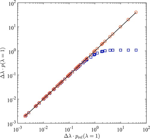
To map all results in a single plot, the corresponding bin size $\mathrm{\Delta }\lambda =1/N_{\mathrm{b}}$ is used as a scaling factor to scale $p\left(\lambda \right)$ at every temperature. The scaled probabilities are shown in Figure 2. The advantage of this representation is that the results obtained at multiple temperatures can be shown in a single plot. As an alternative, a plot of $p(\lambda =1)/p_{\mathrm{r}\mathrm{e}\mathrm{f}}(\lambda =1)$ versus $N_{\mathrm{b}}$ for different temperatures is provided in Figure S1 of the Supporting Information. From Figure 2, it is clear that the extrapolation scheme reaches its limitation for $\mathrm{\Delta }\lambda \cdot p(\lambda =1)\le 1$. In Figure 2 it is observed clearly that the performance of the extrapolation scheme depends both on $\mathrm{\Delta }\lambda =1/N_{\mathrm{b}}$ and the steepness of the distribution $p\left(\lambda \right)$. This means that in sharp contrast to the direct sampling, the accuracy of the extrapolation scheme strongly relies on $\mathrm{\Delta }\lambda \cdot p\left(\lambda \right)$, especially when $p\left(\lambda \right)$ is steep. As shown in Figure 2, the values for $\mathrm{\Delta }\lambda \cdot p(\lambda =1)$ obtained from direct sampling scheme are in excellent agreement with the reference values.

Figure 2. Comparison of scaled $p(\lambda =1)$ for the 2-atom model system in the temperature range between $T^{\ast }=0.005$ and $T^{\ast }=2$, using different number of bins ranging from 10 to 500. To map all results for all temperatures in a single plot, for each system, the corresponding bin size $\mathrm{\Delta }\lambda$ is used as a scaling factor for $p(\lambda =1)$. Alternatively, a plot of $p(\lambda =1)/p_{\mathrm{r}\mathrm{e}\mathrm{f}}(\lambda =1)$ versus $N_{\mathrm{b}}$ for different temperatures is provided in Figure S1 of the Supporting Information. The vertical axis is used for the scaled probabilities obtained based on the extrapolation scheme (squares) and direct sampling (circles). The horizontal axis is used for the reference scaled probabilities $\mathrm{\Delta }\lambda p_{\mathrm{r}\mathrm{e}\mathrm{f}}(\lambda =1)$ obtained from very long MC simulations, using direct sampling (thereby eliminating systematic errors). Raw data are listed in Tables S2 and S3 in the Supporting Information.

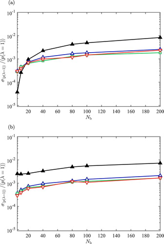
The relative uncertainties of $p(\lambda =1)$ obtained from the simulations of the 2-atom model system are shown in Figure 3, as a function of number of the bins. σ is the uncertainty of $p(\lambda =1)$. It is clear that for small $N_{\mathrm{b}}$, the relative uncertainties obtained using the extrapolation scheme are smaller compared to those obtained from the direct sampling. This indicates that the results obtained from the extrapolation scheme may be more precise but less accurate. For large $N_{\mathrm{b}}$ the relative uncertainties for both methods are very similar. Very similar results for $p\left(\lambda \right)=1$ are obtained for both methods when $N_{\mathrm{b}}$ is large. Based on the results obtained from the 2-atom model system, it is obvious that the direct sampling scheme is the best method with the least dependence on $N_{\mathrm{b}}$. This is an important advantage as it may be difficult to a priori know the best value for $N_{\mathrm{b}}$ for the other schemes.

Figure 3. Relative uncertainty computed for the sampled $p(\lambda =1)$ for the 2-atom model system, ${\sigma }_{p(\lambda =1)}/⟨p(\lambda =1)⟩$, using (a) linear extrapolation, Equation (4(4) ${\mu }^{\mathrm{e}\mathrm{x}}=-\frac{1}{\beta }\ln \left(\frac{p(\lambda \uparrow 1)}{p(\lambda \downarrow 0)}\right).$(4) ), and (b) the direct sampling scheme, Equation (5(5) $\begin{array}{r}{\lambda }^{\ast }\left(\lambda \right)\equiv \left\{\begin{array}{ll}0,& \lambda <\frac{1}{N_{\mathrm{b}}}\\ \frac{N_{\mathrm{b}}\lambda -1}{N_{\mathrm{b}}-2},\frac{1}{N_{\mathrm{b}}}\le & \lambda \le \frac{N_{\mathrm{b}}-1}{N_{\mathrm{b}}}\\ 1,& \lambda >\frac{N_{\mathrm{b}}-1}{N_{\mathrm{b}}}\end{array}\right.\end{array}$(5) ) as a function of number of the bins. The simulations are performed at reduced temperatures: $T^{\ast }=0.05$ (filled triangles), $T^{\ast }=0.5$ (upward-pointing triangles), $T^{\ast }=1.0$ (squares) and $T^{\ast }=1.5$ (down-ward pointing triangles).

As an example of a system with strong LJ and electrostatic interactions, the excess chemical potential of SPC/E water is computed at T=323.15 K and P=1 bar, in the CFCNPT ensemble. The probabilities $p(\lambda \downarrow 0)$ and $p(\lambda \uparrow 1)$ are computed using extrapolation scheme, and $p({\lambda }^{\ast }=0)$ and $p({\lambda }^{\ast }=1)$ are obtained from the direct sampling. The excess chemical potential of water is computed using Equation (4(4) ${\mu }^{\mathrm{e}\mathrm{x}}=-\frac{1}{\beta }\ln \left(\frac{p(\lambda \uparrow 1)}{p(\lambda \downarrow 0)}\right).$(4) ) for extrapolation, and Equation (6(6) ${\mu }^{\mathrm{e}\mathrm{x}}=-\frac{1}{\beta }\ln \left(\frac{p({\lambda }^{\ast }\left(\lambda \right)=1)}{p({\lambda }^{\ast }\left(\lambda \right)=0)}\right).$(6) ) for the direct sampling. The simulations in the CFCNPT ensemble are repeated for different $N_{\mathrm{b}}$ ranging from 5 to 100. The distributions $p\left(\lambda \right)$ are scaled with $\mathrm{\Delta }\lambda =1/N_{\mathrm{b}}$ and the results are shown in Figure 4. Alternatively, plots of $p\left(\lambda \right)/p_{\mathrm{r}\mathrm{e}\mathrm{f}}\left(\lambda \right)$ versus $N_{\mathrm{b}}$ for $p(\lambda =0)$ and $p(\lambda =1)$ are provided in Figure S2 of the Supporting Information. Raw data for Figure 4 are provided in Tables S4 to S7 of the Supporting Information. In Figure 4(a), overall good agreement between all methods is observed except for one outlier for the extrapolation scheme for very few bins ($N_{\mathrm{b}}=5$). This means selecting five bins for the entire λ space is not sufficient even for extrapolation to $\lambda \to 0$ where $p\left(\lambda \right)$ is relatively flat. The distributions $p\left(\lambda \right)$ and $p\left({\lambda }^{\ast }\right)$ for water are shown in Figures S3 and S4 of the Supporting Information. The choice of five bins may not be practical for CFCMC simulation, but it is considered here only to investigate the limitations of Equations (6(6) ${\mu }^{\mathrm{e}\mathrm{x}}=-\frac{1}{\beta }\ln \left(\frac{p({\lambda }^{\ast }\left(\lambda \right)=1)}{p({\lambda }^{\ast }\left(\lambda \right)=0)}\right).$(6) ) and (4(4) ${\mu }^{\mathrm{e}\mathrm{x}}=-\frac{1}{\beta }\ln \left(\frac{p(\lambda \uparrow 1)}{p(\lambda \downarrow 0)}\right).$(4) ). The scaled probabilities of $\lambda =1$ are shown in Figure 4(b). The performances of both methods to obtain $p(\lambda =1)$ for water are very similar to what is observed for the 2-atom model system, as shown Figures 2 and 4. The results of the extrapolation scheme deviate significantly from the reference values when $\mathrm{\Delta }\lambda \cdot p(\lambda =1)>1$. The direct sampling scheme is clearly the best method to calculate $p(\lambda =0)$ and $p(\lambda =1)$. The excess chemical potential of water is calculated based on the extrapolation scheme using Equation (4(4) ${\mu }^{\mathrm{e}\mathrm{x}}=-\frac{1}{\beta }\ln \left(\frac{p(\lambda \uparrow 1)}{p(\lambda \downarrow 0)}\right).$(4) ), and the direct sampling using Equation (6(6) ${\mu }^{\mathrm{e}\mathrm{x}}=-\frac{1}{\beta }\ln \left(\frac{p({\lambda }^{\ast }\left(\lambda \right)=1)}{p({\lambda }^{\ast }\left(\lambda \right)=0)}\right).$(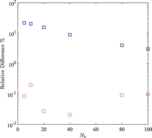6) ). The results are compared to a reference simulations that are 10 times longer, where the excess chemical potential is obtained based on the direct sampling scheme. The relative difference between both methods and the reference are shown in Figure 5. It can be seen in Figure 5 that the accuracy of the extrapolation scheme improves with increasing $N_{\mathrm{b}}$, while the accuracy of direct sampling scheme is hardly influenced by a change in $N_{\mathrm{b}}$. However, very large values of $N_{\mathrm{b}}$ makes computing ${\mu }^{\mathrm{e}\mathrm{x}}$ more difficult as the statistics of the computed occupancy of the bins of $p\left(\lambda \right)$ are reduced. As shown in Figure S5 of the Supporting Information, the free energy barrier as a function of λ that the system needs to overcome is about $12k_{\mathrm{B}}T$ at T=323 K. Using fewer bins for the weight function increases the free energy barrier between adjacent λ bins, which affects the statistics. Increasing the number of bins results in decreasing the free energy barrier between adjacent bins. However, increasing the number of bins also decreases the statistics of the computed occupancy of bins. The relative difference with respect to the reference values observed for the direct sampling scheme is about one to two orders of magnitude smaller compared to those for the extrapolation scheme. The results clearly show that the direct sampling scheme outperforms the extrapolation scheme. The Boltzmann probability distribution of $p\left(\lambda \right)$ for water and methanol in equimolar water–methanol mixture at T=323.15 K and P=1 bar are also shown in Figure S6 of the Supporting Information.

Figure 4. Comparison of the scaled probability distributions (a): $p\left(\lambda \right)=0$ and (b): $p(\lambda =1)$ for the SPC/E water at T=323 K and P=1 bar, using different number of bins ranging from 5 to 100. To map all results in a single plot, for each system, the corresponding bin size $\mathrm{\Delta }\lambda$ is used as a scaling factor for $p(\lambda =0)$ and $p(\lambda =1)$. Alternatively, plots of $p\left(\lambda \right)/p_{\mathrm{r}\mathrm{e}\mathrm{f}}\left(\lambda \right)$ versus $N_{\mathrm{b}}$ for $p(\lambda =0)$ and $p(\lambda =1)$ are provided in Figure S2 of the Supporting Information. The vertical axis is used for the scaled probabilities obtained based on the extrapolation scheme (squares) and direct sampling (circles). The horizontal axis is used for the reference scaled probabilities $p_{\mathrm{r}\mathrm{e}\mathrm{f}}(\lambda =0)$ and $\mathrm{\Delta }\lambda p_{\mathrm{r}\mathrm{e}\mathrm{f}}(\lambda =1)$ obtained longer MC simulations, using direct sampling. Raw data are listed in Tables S4 to S6 in the Supporting Information.

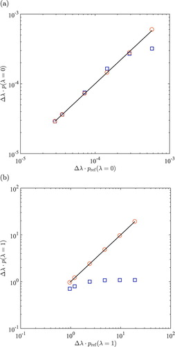
Figure 5. Relative difference (in percent) in the computed excess chemical potential of SPC/E water at T=323 K and P=1 bar using the extrapolation scheme Equation (4(4) ${\mu }^{\mathrm{e}\mathrm{x}}=-\frac{1}{\beta }\ln \left(\frac{p(\lambda \uparrow 1)}{p(\lambda \downarrow 0)}\right).$(4) ) (squares), and the direct sampling Equation (6(6) ${\mu }^{\mathrm{e}\mathrm{x}}=-\frac{1}{\beta }\ln \left(\frac{p({\lambda }^{\ast }\left(\lambda \right)=1)}{p({\lambda }^{\ast }\left(\lambda \right)=0)}\right).$(6) ) (circles). The chemical potential obtained using direct sampling from longer MC simulations is considered as the reference value for the chemical potential. The raw data are provided in Table S7 of the Supporting Information.

To investigate the correlation between the fractional molecules, simulations in the CFCNPT ensemble of LJ colour mixtures with multiple fractional molecules are carried out at a reduced temperature of $T^{\ast }=2$ and a reduced pressure of $P^{\ast }=6$. The simulations are repeated by keeping the number of whole molecules constant (800) while changing $N_{\mathrm{f}\mathrm{r}\mathrm{a}\mathrm{c}}$ between 3 and 50. The instantaneous λ's for two randomly selected fractional molecules are recorded every 100 MC cycles. Simulations are performed both with and without biasing. Calculation of the optimal biasing leads to a flat distribution in λ space during the simulation, the so-called observed $p\left({\lambda }_i\right)$, denoted by $p_{\mathrm{o}\mathrm{b}\mathrm{s}}\left({\lambda }_i\right)$. It is expected that the average $⟨{\lambda }_i⟩$ is close to 0.5 when an optimum biasing is used.  Equation (10(10) $\mathrm{Corr}\left({\lambda }_1,{\lambda }_2\right)=\frac{⟨{\lambda }_1{\lambda }_2⟩-⟨{\lambda }_1⟩⟨{\lambda }_2⟩}{\sqrt{\left[⟨{\lambda }_1^2⟩-{⟨{\lambda }_1⟩}^2\right]\left[⟨{\lambda }_2^2⟩-{⟨{\lambda }_2⟩}^2\right]}},$(10) ) is used to calculate the covariance between the two randomly selected coupling parameters and the results are shown in Table 2. The correlation between ${\lambda }_1$ and ${\lambda }_2$ is very weak independent of the biasing. The averages $⟨{\lambda }_1⟩$ and $⟨{\lambda }_2⟩$ are around 0.5 for the simulations when biasing is used. The correlation between for ${\lambda }_1$ and ${\lambda }_2$ is very weak for all the systems studied, independent of the number of the fractional molecules present in the system. The changes in the correlation between ${\lambda }_1$ and ${\lambda }_2$ appear to be very small and random with respect to changes in $N_{\mathrm{f}\mathrm{r}\mathrm{a}\mathrm{c}}$. ${\lambda }_1$ and ${\lambda }_2$ are also weakly correlated when no biasing is used ($W\left(\lambda \right)=0$), as shown in Table 2. Obviously, the average $⟨{\lambda }_i⟩\ne 0.5$ when no biasing is used (except for ideal gas). It is clear that the coupling parameters are not correlated in simulations in the CFCNPT ensemble, independent of the weight function $W\left(\lambda \right)$. No significant change in the correlation between ${\lambda }_1$ and ${\lambda }_2$ is observed when varying $N_{\mathrm{f}\mathrm{r}\mathrm{a}\mathrm{c}}$.

Table 2. Correlations between two randomly selected fractional molecules in a LJ colour mixture at $T^{\ast }=2$ and $P^{\ast }=6$.

$N_{\mathrm{f}\mathrm{r}\mathrm{a}\mathrm{c}}$	$⟨{\lambda }_1⟩$	$⟨{\lambda }_2⟩$	$⟨{\lambda }_1^2⟩$	$⟨{\lambda }_2^2⟩$	$⟨{\lambda }_1{\lambda }_2⟩$	$\left|\mathrm{C}\mathrm{o}\mathrm{r}\mathrm{r}\right({\lambda }_1,{\lambda }_2\left)\right|$
when $p_{\mathrm{o}\mathrm{b}\mathrm{s}}\left(\lambda \right)$ is flat
3	0.520	0.496	0.355	0.329	0.254	0.046
5	0.512	0.499	0.341	0.331	0.254	0.010
8	0.522	0.500	0.353	0.333	0.257	0.048
10	0.495	0.502	0.327	0.338	0.253	0.061
20	0.518	0.488	0.353	0.323	0.252	0.014
50	0.514	0.528	0.347	0.359	0.273	0.019
$W\left(\lambda \right)=0$
3	0.160	0.157	0.073	0.069	0.026	0.010
5	0.138	0.145	0.057	0.062	0.020	0.010
8	0.144	0.152	0.057	0.063	0.023	0.042
10	0.159	0.145	0.072	0.061	0.022	0.027
20	0.154	0.144	0.065	0.060	0.021	0.019
50	0.151	0.153	0.067	0.065	0.023	0.007

Notes: The system has a constant number of 800 whole LJ molecules, and $N_{\mathrm{f}\mathrm{r}\mathrm{a}\mathrm{c}}$ is the number of the fractional molecules in each simulation. In simulations with non-zero biasing, an independent biasing is calculated for each fractional molecule. The biasing is set such that the observed probability distribution of every fractional molecule, $p_{\mathrm{o}\mathrm{b}\mathrm{s}}\left(\lambda \right)$, is flat.

As an example of a atomistic system with electrostatic interactions, in an equimolar water–methanol mixture of water–methanol the correlation between the fractional molecules of water and methanol is studied. The results are obtained by performing simulations in the CFCNPT ensemble. Coupling parameters ${\lambda }_1$ and ${\lambda }_2$ are assigned to the fractional molecules of water and methanol, respectively. It is clear from Table 3 that ${\lambda }_1$ and ${\lambda }_2$ are very weakly correlated or essentially uncorrelated. In the simulation of water–methanol with non-zero biasing, the averages $⟨{\lambda }_1⟩$ and $⟨{\lambda }_2⟩$ are close to 0.5. This is due to the fact that the observed $p\left(\lambda \right)$ for water and methanol is flat. The values for $⟨{\lambda }_1⟩$ and $⟨{\lambda }_2⟩$ are very close to 1 when the weight function $W\left(\lambda \right)$ is zero. This is due to the fact that the interactions between the fractional molecules and the whole molecules are most favourable when the value of the coupling parameters are close to 1. Figures for $p\left(\lambda \right)$ and $W\left(\lambda \right)$ for water–methanol simulations are provided in Figs. S3 and S4 of the Supporting Information. Since the fractional molecules are not correlated, we can verify that the approximation of Equation (8(8) $W\left({\lambda }_1,{\lambda }_2,\dots {\lambda }_{N_{\mathrm{f}\mathrm{r}\mathrm{a}\mathrm{c}}}\right)\approx \sum _{i=1}^{N_{\mathrm{f}\mathrm{r}\mathrm{a}\mathrm{c}}}{W}_i\left({\lambda }_i\right).$(8) ) is valid.

Table 3. Correlations between the fractional molecules of SPC/E water and traPPE methanol at T=323.15 k and P=1 bar.

$N_{\mathrm{f}\mathrm{r}\mathrm{a}\mathrm{c}}$	$⟨{\lambda }_1⟩$	$⟨{\lambda }_2⟩$	$⟨{\lambda }_1^2⟩$	$⟨{\lambda }_2^2⟩$	$⟨{\lambda }_1{\lambda }_2⟩$	$\left|\mathrm{C}\mathrm{o}\mathrm{r}\mathrm{r}\right({\lambda }_1,{\lambda }_2\left)\right|$
when $p_{\mathrm{o}\mathrm{b}\mathrm{s}}\left(\lambda \right)$ is flat
2	0.514	0.458	0.350	0.295	0.237	0.020
$W\left(\lambda \right)=0$
2	0.989	0.980	0.978	0.961	0.969	0.039

Notes: ${\lambda }_1$ is the fractional molecule of SPC/E water, and ${\lambda }_2$ is the fractional molecule of traPPE rigid methanol. In simulations with non-zero biasing, an independent biasing is calculated for each fractional molecule. The biasing is set such that the observed probability distribution of every fractional molecule, $p_{\mathrm{o}\mathrm{b}\mathrm{s}}\left(\lambda \right)$, is flat.

To investigate the effect of biasing on sampling Boltzmann averages (Equation (9(9) ${⟨X⟩}_{\mathrm{B}\mathrm{o}\mathrm{l}\mathrm{t}\mathrm{z}\mathrm{m}\mathrm{a}\mathrm{n}\mathrm{n}}=\frac{{⟨X\exp \left[-\sum _{i=1}^{N_{\mathrm{f}\mathrm{r}\mathrm{a}\mathrm{c}}}{W}_i\left({\lambda }_i\right)\right]⟩}_{\mathrm{C}\mathrm{F}\mathrm{C}\mathit{N}\mathit{P}\mathit{T}}}{{⟨\exp \left[-\sum _{i=1}^{N_{\mathrm{f}\mathrm{r}\mathrm{a}\mathrm{c}}}{W}_i\left({\lambda }_i\right)\right]⟩}_{\mathrm{C}\mathrm{F}\mathrm{C}\mathit{N}\mathit{P}\mathit{T}}}.$(9) )) two LJ colour mixtures are considered in which 1 and 5 fractional molecules are present, respectively. The optimum biasing is calculated using the Wang-Landau algorithm at $P^{\ast }=6$ and $T^{\ast }=2$. During the simulations, the instantaneous weight factor $\exp [-\sum _{i=1}^{N_{\mathrm{f}\mathrm{r}\mathrm{a}\mathrm{c}}}{W}_i\left({\lambda }_i\right)]$ for both systems is recorded every 100 cycles and the results are shown in Figure 6. The instantaneous weight factor is the statistical weight of a sample system state. It is shown in Figure 6 that the statistical weight for the system including five fractional molecules fluctuates mostly between ${10}^{-9}$ and ${10}^{-4}$, and quite rarely, between ${10}^{-4}$ and ${10}^{-2}$. Multiplying any observable X by such a small number (weight) results in very small numbers, or practically ‘zero’, resulting in poor statistics for $⟨X{⟩}_{\mathrm{B}\mathrm{o}\mathrm{l}\mathrm{t}\mathrm{z}\mathrm{m}\mathrm{a}\mathrm{n}\mathrm{n}}$. The sum of weights in the denominator of Equation (9(9) ${⟨X⟩}_{\mathrm{B}\mathrm{o}\mathrm{l}\mathrm{t}\mathrm{z}\mathrm{m}\mathrm{a}\mathrm{n}\mathrm{n}}=\frac{{⟨X\exp \left[-\sum _{i=1}^{N_{\mathrm{f}\mathrm{r}\mathrm{a}\mathrm{c}}}{W}_i\left({\lambda }_i\right)\right]⟩}_{\mathrm{C}\mathrm{F}\mathrm{C}\mathit{N}\mathit{P}\mathit{T}}}{{⟨\exp \left[-\sum _{i=1}^{N_{\mathrm{f}\mathrm{r}\mathrm{a}\mathrm{c}}}{W}_i\left({\lambda }_i\right)\right]⟩}_{\mathrm{C}\mathrm{F}\mathrm{C}\mathit{N}\mathit{P}\mathit{T}}}.$(9) ) is also a very small number close to zero. This is the aforementioned numerical problem of $\frac{0}{0}$ when computing Boltzmann averages using Equation (9(9) ${⟨X⟩}_{\mathrm{B}\mathrm{o}\mathrm{l}\mathrm{t}\mathrm{z}\mathrm{m}\mathrm{a}\mathrm{n}\mathrm{n}}=\frac{{⟨X\exp \left[-\sum _{i=1}^{N_{\mathrm{f}\mathrm{r}\mathrm{a}\mathrm{c}}}{W}_i\left({\lambda }_i\right)\right]⟩}_{\mathrm{C}\mathrm{F}\mathrm{C}\mathit{N}\mathit{P}\mathit{T}}}{{⟨\exp \left[-\sum _{i=1}^{N_{\mathrm{f}\mathrm{r}\mathrm{a}\mathrm{c}}}{W}_i\left({\lambda }_i\right)\right]⟩}_{\mathrm{C}\mathrm{F}\mathrm{C}\mathit{N}\mathit{P}\mathit{T}}}.$(9) ). For the system including a single fractional molecule, the weight fluctuates between ${10}^{-2}$ to ${10}^0$ during the simulation. Based on Figure 6, it can be concluded that the uncertainty in the Boltzmann average of any observable X increases with the increase in the number of fractional molecules.

Figure 6. Instantaneous weight factor, $\exp [-\sum _{i=1}^{N_F}{W}_i\left({\lambda }_i\right)]$, for a LJ system with 1 fractional molecule (triangles) and 5 fractional molecules (circles), at $T^{\ast }=2$ and $P^{\ast }=6$. $W_i\left({\lambda }_i\right)$ is set such that $p_{\mathrm{o}\mathrm{b}\mathrm{s}}\left({\lambda }_i\right)$ for every fractional molecule is flat.

One possible solution to circumvent the sampling of Boltzmann averages in simulations with multiple fractional molecules, is to directly sample the averages without removing the biasing (Equation (3(3) ${⟨X⟩}_{\mathrm{B}\mathrm{i}\mathrm{a}\mathrm{s}\mathrm{e}\mathrm{d}}=\frac{\sum _{i=1}^{N_{\mathrm{S}}}X}{N_{\mathrm{S}}},$(3) )). $⟨X{⟩}_{\mathrm{b}\mathrm{i}\mathrm{a}\mathrm{s}\mathrm{e}\mathrm{d}}$ is the average of observable X in simulations in the CFCMC ensemble. To compare the statistics of the Boltzmann and biased averages, we have selected the average volume of the system in the CFCNPT simulations. The Boltzmann and biased ensemble averages of volume obtained from the CFCNPT ensemble simulations, with $p{r}_{\mathrm{f}}$ between 0.125% and 6.25%, are calculated for $P^{\ast }=1$ and $P^{\ast }=6$. $p{r}_{\mathrm{f}}$ is the ratio between the number of the fractional molecules with respect to the number of the whole molecules, expressed as a percentage. The Boltzmann average of volume in the NPT is computed for the same number of whole molecules at the same temperature and pressure as a reference value. The relative uncertainty of the volume of every system is shown in Figure 7 as a function of $p{r}_{\mathrm{f}}$. The normalised uncertainty of the volume obtained from the NPT ensemble simulations is shown on the vertical axis. It is shown in Figure 7(a) that at a number density $⟨{\rho }^{\ast }{⟩}_{\mathit{N}\mathit{P}\mathit{T}}=0.43$, the normalised uncertainties of the Boltzmann and biased averages of the volume are very similar for $p{r}_{\mathrm{f}}\le 1.25$%. Good agreement is observed with the results from the NPT ensemble simulations. However, poor statistics are observed for increasing $p{r}_{\mathrm{f}}$. As shown in Figure 7(b), the differences between the averages obtained from Equations (9(9) ${⟨X⟩}_{\mathrm{B}\mathrm{o}\mathrm{l}\mathrm{t}\mathrm{z}\mathrm{m}\mathrm{a}\mathrm{n}\mathrm{n}}=\frac{{⟨X\exp \left[-\sum _{i=1}^{N_{\mathrm{f}\mathrm{r}\mathrm{a}\mathrm{c}}}{W}_i\left({\lambda }_i\right)\right]⟩}_{\mathrm{C}\mathrm{F}\mathrm{C}\mathit{N}\mathit{P}\mathit{T}}}{{⟨\exp \left[-\sum _{i=1}^{N_{\mathrm{f}\mathrm{r}\mathrm{a}\mathrm{c}}}{W}_i\left({\lambda }_i\right)\right]⟩}_{\mathrm{C}\mathrm{F}\mathrm{C}\mathit{N}\mathit{P}\mathit{T}}}.$(9) ) and (3(3) ${⟨X⟩}_{\mathrm{B}\mathrm{i}\mathrm{a}\mathrm{s}\mathrm{e}\mathrm{d}}=\frac{\sum _{i=1}^{N_{\mathrm{S}}}X}{N_{\mathrm{S}}},$(3) ) are more pronounced at higher densities ($⟨{\rho }^{\ast }{⟩}_{\mathit{N}\mathit{P}\mathit{T}}=0.80$). It is observed in Figure 7(b) that the sampling of the Boltzmann average of the volume is significantly affected with increasing $p{r}_{\mathrm{f}}$, in sharp contrast to the biased averages. The uncertainty of the biased average of volume does not change significantly for increasing $p{r}_{\mathrm{f}}$. This is due to the aforementioned $\frac{0}{0}$ sampling problem. Excellent agreement is observed between the relative uncertainties of biased averages of volume and the results obtained from the NPT ensemble. Raw data for Figure 7 are provided in Tables 5 and 4.

Figure 7. Relative uncertainty of the Boltzmann averages of the volume, $\sigma /⟨V⟩$, (triangles) and the biased averages of volume (circles) in the CFCNPT ensemble, at (a) $T^{\ast }=2$, $P^{\ast }=1$ and (b) $T^{\ast }=2$, $P^{\ast }=6$. $p{r}_{\mathrm{f}}$ is the ratio between the number of the fractional molecules with respect to the number of the whole molecules (constant 800), expressed as a percentage. The relative uncertainty of V is defined as the ratio of the uncertainty of the volume ${\sigma }_V$ to the mean volume $⟨V⟩$. The arrows on the left indicate the value of the relative uncertainty of volume obtained from the NPT simulations, on the vertical axes. Raw data are provided in Tables 5 and 4.

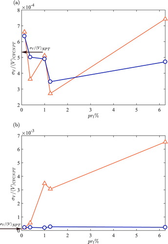
Table 4. Relative differences between Boltzmann averages obtained from CFCNPT simulations and Boltzmann averages obtained from NPT simulations of different LJ colour mixtures, at $T^{\ast }=2$ and reduced pressures between $P^{\ast }=0.5$ to $P^{\ast }=6$.

$p{r}_{\mathrm{f}}$	$⟨E{⟩}_{\mathrm{C}\mathrm{F}\mathrm{C}\mathit{N}\mathit{P}\mathit{T}}$	$⟨V{⟩}_{\mathrm{C}\mathrm{F}\mathrm{C}\mathit{N}\mathit{P}\mathit{T}}$	${\eta }_E$	${\eta }_{\rho }$	${\eta }_V$	${\mu }_1^{\mathrm{e}\mathrm{x}}$	$⟨{\mu }_i^{\mathrm{e}\mathrm{x}}⟩$
$P^{\ast }=0.5$
0.125	−1130.2(9)	3042(2)	0.04	0.15	0.15	−0.37(3)	−0.37(3)
0.375	−1129.4(6)	3051(2)	0.11	0.45	0.45	−0.40(2)	−0.38(2)
1.00	−1127.1(6)	3074(2)	0.32	1.22	1.23	−0.37(5)	−0.38(3)
1.25	−1125.5(5)	3085(2)	0.46	1.55	1.58	−0.37(5)	−0.37(3)
6.25	−1109.1(9)	3272(2)	1.95	7.18	7.74	−0.4(2)	−0.34(1)
$P^{\ast }=1$
0.125	−1820(2)	1852(1)	0.03	0.13	0.13	0.07(2)	0.07(2)
0.375	−1818(1)	1857(1)	0.09	0.40	0.40	0.08(2)	0.07(3)
1.00	−1816(1)	1869(1)	0.22	1.04	1.05	0.07(6)	0.07(2)
1.25	−1816(1)	1873(1)	0.23	1.25	1.26	0.0(1)	0.07(2)
6.25	−1800(2)	1970(1)	1.14	6.08	6.48	0.1(1)	0.08(2)
$P^{\ast }=6$
0.125	−3126.7(9)	998.9(2)	0.03	0.03	0.03	6.39(5)	6.39(5)
0.375	−3125(2)	999(1)	0.07	0.09	0.09	6.41(5)	6.43(3)
1.00	−3113(13)	1002(3)	0.47	0.30	0.30	6.32(6)	6.41(3)
1.25	−3126(13)	1001(3)	0.06	0.24	0.24	6.32(6)	6.38(3)
6.25	−3085(42)	1033(7)	1.38	3.30	3.42	6.4(2)	6.38(2)

Notes: $p{r}_{\mathrm{f}}$ is the ratio between the number of the fractional molecules with respect to the number of the whole molecules (constant 800), expressed as a percentage. The ensemble averages for energy and volume obtained from the NPT ensemble simulations, in reduced units, equal $-1130.7\left(8\right)$ and $3037\left(2\right)$ for $P^{\ast }=0.5$, $-1820\left(1\right)$ and $1850\left(1\right)$, for $P^{\ast }=1$, $-3127.7\left(8\right)$ and $998.6\left(8\right)$ for $P^{\ast }=6$, respectively. In the table below, ${\eta }_X$ is the difference of the boltzmann average $⟨x{⟩}_{\mathrm{C}\mathrm{F}\mathrm{C}\mathit{N}\mathit{P}\mathit{T}}$ with respect to $⟨x{⟩}_{NPT}$, expressed as a percentage. for colour mixtures with multiple fractional molecules, ${\mu }_1^{\mathrm{e}\mathrm{x}}$ is the excess chemical potential of a randomly selected fractional molecule, in reduced units, and $⟨{\mu }_i^{\mathrm{e}\mathrm{x}}⟩$ is the excess chemical potential averaged over all the fractional molecules. Numbers in brackets are uncertainties in the last digit, i.e. −0.37(3) means −0.37 ± 0.03.

Table 5. Relative difference between the biased averages obtained from the CFCNPT simulations and boltzmann averages obtained from the NPT simulations of different LJ colour mixtures, at $T^{\ast }=2$ and reduced pressures between $P^{\ast }=0.5$ to $P^{\ast }=6$. $p{r}_{\mathrm{f}}$ is the ratio between the number of the fractional molecules with respect to the number of the whole molecules (constant 800), expressed as a percentage.

$p{r}_{\mathrm{f}}$	$⟨E{⟩}_{\mathrm{C}\mathrm{F}\mathrm{C}\mathit{N}\mathit{P}\mathit{T}}$	$⟨V{⟩}_{\mathrm{C}\mathrm{F}\mathrm{C}\mathit{N}\mathit{P}\mathit{T}}$	${\eta }_E$	${\eta }_{\rho }$	${\eta }_V$
$P^{\ast }=0.5$
0.125	−1130(1)	3042(3)	0.07	0.15	0.15
0.375	−1128.9(8)	3051(2)	0.15	0.47	0.47
1	−1126(1)	3075(3)	0.41	1.23	1.25
1.25	−1124.3(8)	3086(2)	0.56	1.58	1.61
6.25	−1103.4(7)	3276(2)	2.41	7.31	7.88
$P^{\ast }=1$
0.125	−1819(1)	1853(1)	0.06	0.17	0.17
0.375	−1819(1)	1857.4(9)	0.10	0.40	0.40
1	−1816(1)	1869.4(9)	0.24	1.03	1.04
1.25	−1814.1(7)	1874.9(7)	0.35	1.33	1.34
6.25	−1791(1)	1975.5(9)	1.61	6.35	6.78
$P^{\ast }=6$
0.125	−3126(1)	998.9(2)	0.04	0.03	0.03
0.375	−3127(1)	1001.2(2)	0.02	0.26	0.26
1	−3126(1)	1005.7(2)	0.07	0.71	0.71
1.25	−3125(2)	1007.6(3)	0.10	0.89	0.90
6.25	−3117(1)	1043.4(2)	0.36	4.29	4.49

Notes: The ensemble averages for energy and volume obtained from the NPT ensemble simulations, in reduced units, equal $-1130.7\left(8\right)$ and $3037\left(2\right)$ for $P^{\ast }=0.5$, $-1820\left(1\right)$ and $1850\left(1\right)$, for $P^{\ast }=1$, $-3127.7\left(8\right)$ and $998.6\left(8\right)$ for $P^{\ast }=6$, respectively. In the table below, ${\eta }_X$ is the difference of the biased average $⟨x{⟩}_{\mathrm{C}\mathrm{F}\mathrm{C}\mathit{N}\mathit{P}\mathit{T}}$ with respect to $⟨x{⟩}_{NPT}$, expressed as a percentage. numbers in brackets are uncertainties in the last digit, i.e. −0.37(3) means −0.37 ± 0.03.

The results in Figure 7 show that the biased average of volume in the CFCNPT ensemble simulations can be statistically more precise compared to the Boltzmann average of the volume. Therefore, it is instructive to investigate the difference between the Boltzmann and biased averages obtained from the CFCNPT simulations, with multiple fractional molecules, and the Boltzmann averages obtained from the conventional NPT ensemble. This may provide guidelines for how many fractional molecules are allowed before the Boltzmann/biased averages significantly deviate from those obtained from the conventional NPT ensemble simulations. Note that by increasing the number of fractional molecules, we are investigating the performance of the CFCMC method in extreme cases. In most practical applications $N_{\mathrm{f}\mathrm{r}\mathrm{a}\mathrm{c}}$ is usually smaller than five which means that $p{r}_{\mathrm{f}}$ is significantly smaller than 1% [3,6,11,25,31,49,51,52,55,75]. For this percentage of fractional molecules, very good estimations for conventional ensemble averages are obtained from CFCMC simulations [3,49,51,52]. For instance, CFCGE simulations of binary or ternary mixtures include at most two or three fractional molecules. For a reactive system of $\mathrm{A}+\mathrm{B}\rightleftharpoons \mathrm{C}+\mathrm{D}$ in the liquid phase where component A is volatile, three fractional molecules are required i.e. two fractional molecules of reactant molecules (A and B) or reaction products (C and D) and a fractional molecule of the type A in the gas phase. We also investigate how the excess chemical potential calculations are affected when $p{r}_{\mathrm{f}}$ increases. For these systems, the excess chemical potential of a randomly selected fractional molecule, ${\mu }_1^{\mathrm{e}\mathrm{x}}$ and the average of all the chemical potentials of all fractional molecules, $⟨{\mu }_i^{\mathrm{e}\mathrm{x}}⟩$ are shown in Table 4. As shown in this table, the uncertainty of ${\mu }_1^{\mathrm{e}\mathrm{x}}$ increases as the number of the fractional molecules in the system increases. This is because the simulation time is divided to perform random walks multidimensional λ space. However, the statistics of the chemical potential averaged over all fractional molecules $⟨{\mu }_i^{\mathrm{e}\mathrm{x}}⟩$ does not depend strongly on the number of fractional molecules in the colour mixture. This is due to the fact that all the intermolecular interactions in the colour mixture are similar. Therefore, the chemical potentials of all the LJ molecules in this simulation are equal.

The relative difference for ensemble averages of the energy, density and the volume in the CFCNPT simulations are compared to Boltzmann averages obtained from the NPT simulations. The results are provided in Tables 4 and 5. At $p^{\ast }=6$, the relative difference for the Boltzmann average of energy increases significantly with the increase in $p{r}_{\mathrm{f}}$, in sharp contrast to the error associated with the biased average of energy. This shows once more that the sampling issue of Boltzmann averages in dense systems with multiple fractional molecules is more pronounced (because of larger biasing). It can be seen in Table 4 that the Boltzmann averages obtained from the CFCNPT ensemble where $p{r}_{\mathrm{f}}\le 1\mathrm{\%}$ are very similar to those obtained from the NPT ensemble. For $p{r}_{\mathrm{f}}=1\mathrm{\%}$, the relative difference for the Boltzmann averages density and volume in the CFCNPT ensemble are about 1% or smaller. We consider 1% as a typical uncertainty from simulations (also differences between experimental data and force field-based simulations are typically also of that order). This applies to normal averages e.g. density, volume etc, but not chemical potentials. The chemical potentials computed by CFCMC and without fractional molecule are usually identical [51]. The relative error for the Boltzmann averages density and volume decreases to 0.3% by increasing the pressure to $P^{\ast }=6$. As shown in Table 5, good agreement is observed between the biased averages from the CFCNPT simulations and the Boltzmann averages from the NPT simulations for $p{r}_{\mathrm{f}}\le 1\mathrm{\%}$ (typical differences are around 1%). The relative difference between the biased averages density and volume obtained from the simulations at $P^{\ast }=1$ and $P^{\ast }=6$ are smaller than 1%. For $P^{\ast }=0.5$, relative difference smaller than 1% are obtained for $p{r}_{\mathrm{f}}\le 0.375\mathrm{\%}$. It can be seen from Tables 4 and 5 that the errors associated with the biased averages are smaller compared to the Boltzmann averages, especially at high densities. Therefore, it is possible to use biased averages in systems where $p{r}_{\mathrm{f}}\le 1\mathrm{\%}$. The advantage is that the statistics of biased averages may be better, depending on the system density, compared to Boltzmann averages. In practice, $N_{\mathrm{f}\mathrm{r}\mathrm{a}\mathrm{c}}$ is nearly always below 5 even for studying complex molecular systems [3,6,11,25,49,51,52,55,75]. This means that for a system of 500 molecules (a relatively small system size), $p{r}_{\mathrm{f}}$ would nearly always be smaller than 1%.

5. Conclusions

An alternative binning scheme is presented to compute the excess chemical potential in CFCMC simulations. This scheme is developed to overcome sampling issues of the excess chemical potential associated with the linear extrapolation to $\lambda \to 0$ and $\lambda \to 1$ used in CFCMC simulations in our earlier work. The drawback of linear extrapolation is that precise values obtained for the excess chemical potential may provide a false impression of accuracy. Increasing the number of bins may improve the accuracy of the extrapolation scheme, however, this leads to poor sampling (larger uncertainty) of $p\left(\lambda \right)$ for a fixed simulation time. It is a priori unclear what the optimum number of bins should be for a certain system. In the alternative binning scheme, the first and the last bins are directly used to sample the probability of the interaction parameters ${\lambda }^{\ast }=0$ (ideal gas behaviour) and ${\lambda }^{\ast }=1$ (fully scaled interactions), respectively. The excess chemical potential is computed by sampling the beginning and end states of λ rigorously (the direct sampling scheme). This method can be implemented in a single step in existing CFCMC codes by performing linear transformation of λ (Equation (5(5) $\begin{array}{r}{\lambda }^{\ast }\left(\lambda \right)\equiv \left\{\begin{array}{ll}0,& \lambda <\frac{1}{N_{\mathrm{b}}}\\ \frac{N_{\mathrm{b}}\lambda -1}{N_{\mathrm{b}}-2},\frac{1}{N_{\mathrm{b}}}\le & \lambda \le \frac{N_{\mathrm{b}}-1}{N_{\mathrm{b}}}\\ 1,& \lambda >\frac{N_{\mathrm{b}}-1}{N_{\mathrm{b}}}\end{array}\right.\end{array}$(5) )) when calculating the interaction potential of the fractional molecule with the surroundings. In sharp contrast to linear extrapolation, the accuracy and precision of this alternative binning scheme does not strongly depend on the number of the bins. As an example of a system with strong intermolecular interactions, we have computed the excess chemical potential of SPC/E water using both methods. We observed that the excess chemical potential is underestimated for SPC/E water using linear extrapolation to $\lambda \to 0$ and $\lambda \to 1$, since $p\left(\lambda \right)$ is steep close to $\lambda =1$. Generally, this steepness is observed for dense systems or systems with large molecules or with strong intermolecular interactions. We found that the direct sampling scheme is the best method for chemical potential calculations. Very weak or no correlation was found between the fractional molecules in multicomponent systems. This allows one to effectively split a multidimensional weight function into a series of one-dimensional weight functions for every fractional molecule. Using this approach, filling a multidimensional histogram of the weight function is avoided, which is computationally not efficient, and a flatness criterion can be applied to each histogram separately. In systems where multiple fractional molecules are present, the weight function is typically large, which leads to the aforementioned $\frac{0}{0}$ numerical problem associated with poor sampling of Boltzmann averages. Our solution is to use biased averages instead of Boltzmann averages. To have similar ensemble averages compared to those obtained from the conventional ensembles, it is recommended that the number of the fractional molecules does not exceed 1% of the total number of molecules. The threshold may be system dependent. In may practical applications, the percentage of fractional molecules is much lower than 1%. To investigate the limits of the CFCMC method, systems with higher percentage of fractional molecules were considered in this work. We have shown that increasing the number of the fractional molecules does not affect the value/accuracy of the excess chemical potential of each fractional molecule.

Disclosure statement

No potential conflict of interest was reported by the authors.

ORCID

A. Rahbari  http://orcid.org/0000-0002-6474-3028

R. Hens  http://orcid.org/0000-0002-6147-0749

D. Dubbeldam  http://orcid.org/0000-0002-4382-1509

T.J.H. Vlugt  http://orcid.org/0000-0003-3059-8712

Additional information

Funding

This work was sponsored by NWO Exacte Wetenschappen (Physical Sciences) for the use of supercomputer facilities, with financial support from the Nederlandse Organisatie voor Wetenschappelijk Onderzoek (Netherlands Organization for Scientific Research, NWO). TJHV acknowledges NWO-CW for a VICI grant.

References

- D. Frenkel and B. Smit, Understanding Molecular Simulation: From Algorithms to Applications, 2nd ed. (Academic Press, San Diego, California, 2002).
- B. Smit and D. Frenkel, Mol. Phys. 68, 951–958 (1989).
- A. Rahbari, A. Poursaeidesfahani, A. Torres-Knoop, D. Dubbeldam and T.J.H. Vlugt, Mol. Simul. 44, 405–414 (2018).
- G. Raabe and E.J. Maginn, J. Phys. Chem. Lett. 1, 93–96 (2010).
- E.J. Maginn, AIChE J. 55, 1304–1310 (2009).
- Q.R. Sheridan, R.G. Mullen, T.B. Lee, E.J. Maginn and W.F. Schneider, J. Phys. Chem. C 122, 14213–14221 (2018).
- M.B. Shiflett and E.J. Maginn, AIChE J. 63, 4722–4737 (2017).
- A.S. Paluch and E.J. Maginn, AIChE J. 59, 2647–2661 (2013).
- E.O. Fetisov and J.I. Siepmann, J. Chem. Eng. Data 59, 3301–3306 (2014).
- T.M. Becker, A. Luna-Triguero, J.M. Vicent-Luna, L.C. Lin, D. Dubbeldam, S. Calero and T.J.H. Vlugt, Phys. Chem. Chem. Phys. 20, 28848–28859 (2018).
- R. Hens and T.J.H. Vlugt, J. Chem. Eng. Data 63 (4), 1096–1102 (2018).
- M.G. Martin and J.I. Siepmann, Theor. Chem. Acc. 99, 347–350 (1998).
- B. Chen, J.I. Siepmann and M.L. Klein, J. Phys. Chem. B 105, 9840–9848 (2001).
- P. Bai and J.I. Siepmann, J. Chem. Theory Comput. 13, 431–440 (2017).
- M. Dinpajooh, P. Bai, D.A. Allan and J.I. Siepmann, J. Chem. Phys. 143, 114113 (2015).
- P. Bai and J.I. Siepmann, Fluid Phase Equilib. 351, 1–6 (2013).
- A. Poursaeidesfahani, M.F. de Lange, F. Khodadadian, D. Dubbeldam, M. Rigutto, N. Nair and T.J.H. Vlugt, J. Catal. 353, 54–62 (2017).
- J.M. Castillo, T.J.H. Vlugt, D. Dubbeldam, S. Hamad and S. Calero, J. Phys. Chem. C 114, 22207–22213 (2010).
- I. Matito-Martos, A. Rahbari, A. Martin-Calvo, D. Dubbeldam, T.J.H. Vlugt and S. Calero, Phys. Chem. Chem. Phys. 20, 4189–4199 (2018).
- E.O. Fetisov, I.F.W. Kuo, C. Knight, J. VandeVondele, T. Van Voorhis and J.I. Siepmann, ACS. Cent. Sci. 2, 409–415 (2016).
- S.P. Balaji, S. Gangarapu, M. Ramdin, A. Torres-Knoop, H. Zuilhof, E.L.V. Goetheer, D. Dubbeldam and T.J.H. Vlugt, J. Chem. Theory Comput. 11 (6), 2661–2669 (2015).
- E.O. Fetisov, M.S. Shah, C. Knight, M. Tsapatsis and J.I. Siepmann, ChemPhysChem 19, 512–518 (2018).
- R.G. Mullen, S.A. Corcelli and E.J. Maginn, J. Phys. Chem. Lett. 9, 5213–5218 (2018).
- R.G. Mullen and E.J. Maginn, J. Chem. Theory Comput. 13, 4054–4062 (2017).
- T.W. Rosch and E.J. Maginn, J. Chem. Theory Comput. 7, 269–279 (2011).
- A.Z. Panagiotopoulos, Mol. Simul. 9 (1), 1–23 (1992).
- A.Z. Panagiotopoulos, Fluid Phase Equilib. 76, 97–112 (1992).
- A.Z. Panagiotopoulos, Mol. Phys. 61, 813–826 (1987).
- B. Widom, J. Chem. Phys. 39, 2808–2812 (1963).
- J. Recht and A. Panagiotopoulos, Mol. Phys. 80, 843–852 (1993).
- A. Torres-Knoop, N.C. Burtch, A. Poursaeidesfahani, S.P. Balaji, R. Kools, F.X. Smit, K.S. Walton, T.J.H. Vlugt and D. Dubbeldam, J. Phys. Chem. C 120, 9148–9159 (2016).
- G.C. Boulougouris, I.G. Economou and D.N. Theodorou, J. Mol. Phys. 96, 905–913 (1999).
- G.C. Boulougouris, I.G. Economou and D.N. Theodorou, J. Comput. Phys. 115 (17), 8231–8237 (2001).
- B. Widom, J. Phys. Chem. 86, 869–872 (1982).
- D.A. Kofke, Fluid Phase Equilib. 228–229, 41–48 (2005).
- A. Torres-Knoop, S.P. Balaji, T.J.H. Vlugt and D. Dubbeldam, J. Chem. Theory Comput. 10, 942–952 (2014).
- G.C.A.M. Mooij and D. Frenkel, J. Phys.: Condens. Matt. 6 (21), 3879–3888 (1994).
- K. Shing and K. Gubbins, Mol. Phys. 49 (5), 1121–1138 (1983).
- K. Shing and K. Gubbins, Mol. Phys. 45 (1), 129–139 (1982).
- K.K. Mon and R.B. Griffiths, Phys. Rev. A 31, 956–959 (1985).
- T.J.H. Vlugt, Mol. Simul. 23, 63–78 (1999).
- D.R. Squire and W.G. Hoover, J. Chem. Phys. 50, 701–706 (1969).
- M.R. Mruzik, F.F. Abraham, D.E. Schreiber and G.M. Pound, J. Chem. Phys. 64, 481–491 (1976).
- F.A. Escobedo and J.J. de Pablo, J. Chem. Phys. 105, 4391–4394 (1996).
- W. Shi and E.J. Maginn, J. Chem. Theory Comput. 3, 1451–1463 (2007).
- W. Shi and E.J. Maginn, J. Comput. Chem. 29, 2520–2530 (2008).
- B. Yoo, E. Marin-Rimoldi, R.G. Mullen, A. Jusufi and E.J. Maginn, Langmuir 33, 9793–9802 (2017).
- A.S. Paluch, J.K. Shah and E.J. Maginn, J. Chem. Theory Comput. 7, 1394–1403 (2011).
- A. Rahbari, R. Hens, I.K. Nikolaidis, A. Poursaeidesfahani, M. Ramdin, I.G. Economou, O.A. Moultos, D. Dubbeldam and T.J.H. Vlugt, Mol. Phys. 116, 3331–3344 (2018).
- B.J. Sikora, Y.J. Coln and R.Q. Snurr, Mol. Simul. 41, 1339–1347 (2015).
- A. Poursaeidesfahani, A. Torres-Knoop, D. Dubbeldam and T.J.H. Vlugt, J. Chem. Theory Comput. 12, 1481–1490 (2016).
- A. Poursaeidesfahani, R. Hens, A. Rahbari, M. Ramdin, D. Dubbeldam and T.J.H. Vlugt, J. Chem. Theory Comput. 13, 4452–4466 (2017).
- F. Wang and D.P. Landau, Phys. Rev. Lett. 86, 2050–2053 (2001).
- P. Poulain, F. Calvo, R. Antoine, M. Broyer and P. Dugourd, Phys. Rev. E 73, 056704 (2006).
- A. Rahbari, R. Hens, S.H. Jamali, M. Ramdin, D. Dubbeldam and T.J.H. Vlugt, Mol. Simul. 45, 336–350 (2019).
- M.R. Shirts and V.S. Pande, J. Chem. Phys. 122, 134508 (2005).
- M.R. Shirts, J.W. Pitera, W.C. Swope and V.S. Pande, J. Chem. Phys. 119, 5740–5761 (2003).
- M.R. Shirts, D.L. Mobley and J.D. Chodera, in Annual Reports in Computational Chemistry, edited by D.C. Spellmeyer and R. Wheeler (Elsevier, United States, 2007), pp. 41–59.
- J.W. Erisman, M.A. Sutton, J. Galloway, Z. Klimont and W. Winiwarter, Nat. Geosci. 1, 636–639 (2008).
- P. Sindzingre, G. Ciccotti, C. Massobrio and D. Frenkel, Chem. Phys. Lett. 136, 35–41 (1987).
- P. Sindzingre, C. Massobrio, G. Ciccotti and D. Frenkel, Chem. Phys. 129, 213–224 (1989).
- S. Caro-Ortiz, R. Hens, E. Zuidema, M. Rigutto, D. Dubbeldam and T.J.H. Vlugt, Fluid Phase Equilib. 485, 239–247 (2019).
- A. Poursaeidesfahani, A. Rahbari, A. Torres-Knoop, D. Dubbeldam and T.J.H. Vlugt, Mol. Simul. 43, 189–195 (2017).
- H.J.C. Berendsen, J.R. Grigera and T.P. Straatsma, J. Phys. Chem. 91, 6269–6271 (1987).
- B. Chen, J.J. Potoff and J.I. Siepmann, J. Phys. Chem. B 105, 3093–3104 (2001).
- C.J. Fennell and J.D. Gezelter, J. Chem. Phys. 124, 234104 (2006).
- D. Wolf, P. Keblinski, S.R. Phillpot and J. Eggebrecht, J. Chem. Phys. 110, 8254–8282 (1999).
- D. Wolf, Phys. Rev. Lett. 68, 3315–3318 (1992).
- C. Waibel and J. Gross, J. Chem. Theory Comput. 14, 2198–2206 (2018).
- C. Waibel, M.S. Feinler and J. Gross, J. Chem. Theory Comput. 15, 572–583 (2019).
- P.V. Klimovich, M.R. Shirts and D.L. Mobley, J Comput. Aided. Mol. Des. 29, 397–411 (2015).
- L.N. Naden, T.T. Pham and M.R. Shirts, J. Chem. Theory Comput. 10, 1128–1149 (2014).
- L.N. Naden and M.R. Shirts, J. Chem. Theory Comput. 11, 2536–2549 (2015).
- M.P. Allen and D.J. Tildesley, Computer Simulation of Liquids, 2nd ed. (Oxford University Press, Oxford, 2017).
- W. Shi and E.J. Maginn, J. Phys. Chem. B 112, 2045–2055 (2008).