Intramolecular bonding in a statistical associating fluid theory of ring aggregates

Abstract

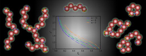
The first-order thermodynamic perturbation theory of Wertheim (TPT1) is extended to treat ring aggregates, formed by inter- and intramolecular association. The expression for the residual association contribution to the Helmholtz free energy for ring aggregates, incorporating the appropriate terms in Wertheim's fundamental graph sum of the TPT1 density expansion, is derived to calculate the distribution of the molecular bonding states. This requires the introduction of two new parameters to characterise each possible ring type: the ring size τ, which is equal to one in the case of intramolecular association, and a parameter W that captures the likelihood of two ring-forming sites bonding. The resulting framework can be incorporated in equations of state that account for the residual association contribution to the free energy, such as the statistical associating fluid theory (SAFT) family, or the cubic plus association (CPA) equation of state. This extends the applicability of these equations of state to mixtures with an arbitrary number of association sites capable of hydrogen bonding to form intramolecular and intermolecular rings. The formalism is implemented within SAFT-VR Mie to calculate the fluid-phase equilibria of model chain-like molecules containing two associating sites A and B, allowing for the formation of open-chain aggregates and intramolecular bonds. The effect of adding a second component that competes for the association sites that mediate intramolecular association in the chain is also examined. Accounting for intramolecular bonding is shown to have a significant impact on the phase equilibria of such systems.

GRAPHICAL ABSTRACT

Keywords:

• Association
• ring formation
• intramolecular association
• hydrogen bonding
• SAFT

1. Introduction

The hydrogen bond (HB) is defined [1] by the International Union of Pure and Applied Chemistry (IUPAC) as an

attractive interaction between a hydrogen atom from a molecule or a molecular fragment X–H in which X is more electronegative than H, and an atom or a group of atoms in the same or a different molecule, in which there is evidence of bond formation.

Hydrogen bonds are characterised by their orientation, usually requiring the participating atoms to be collinear, and by their strength, with energies ranging from 8 kJ mol${}^{-1}$ in the case of weak hydrogen bonds involving π orbitals to more than 40 kJ mol${}^{-1}$ when charged acceptor groups are present [2]. The formation of hydrogen bonds leads to long-lived molecular aggregates that markedly influence the thermodynamic and phase behaviour of the system.

Most commonly, hydrogen bonds form between independent molecules (intermolecular HB), leading to the formation of linear or branched chain-like aggregates or networks that can extend in open form as well as include ring-like structures. In addition, hydrogen bonds may involve atoms in different parts of the same molecule (intramolecular HB), on occasion leading to bent X–H…X conformations in smaller molecules (e.g. Schiff bases) where strong steric constraints result. Hydrogen bonding can also be found within large macromolecules (polymers and proteins) with little constraint from the covalent bonds binding the atoms. The macroscopic manifestations of these two types of HB bond can be rather different and striking. Intermolecular HB are responsible for the high boiling temperatures and heats of vaporisation of small molecules such as water and ammonia, and the re-entrant vapour-phase behaviour reported in patchy colloids is also due to the formation of intermolecular ring-like aggregates [3]. Marked differences in solubility are seen between polar molecules in which intramolecular HBs form, where an enhancement in lipophilicity and cell-membrane permeability is observed [4], and the ‘open’ unbonded forms, which are more water-soluble [5,6]. Furthermore, the folding and aggregation of proteins are directly related to the formation of inter- and intramolecular HB (aggregation of mis-folded proteins is a common feature of diseases such as Alzheimer's, Parkinson's and type II diabetes [7]), as are the binding and specificity of ligands [8,9], the stabilisation of many polymer structures [10–12], and the changes reported in cloud-point pressures of polymer solutions [13,14].

Accounting for the effect of hydrogen bonding and aggregate formation has been of interest for some time in the development of theories for the fluid state. In 1908, Dolezalek [15] proposed a chemical approach to account for hydrogen bonding by considering that molecules aggregate into a new species through a chemical reaction, allowing for an explanation of many of the observed deviations from Raoult's law seen in solutions of associating fluids. The main drawback of Dolezalek's approach is that each of the association aggregates needs to be specified a priori. In the 1970s and 80s the advent of molecular-based association theories [16–25] provided a path towards understanding the distribution of association aggregates. Wertheim [26–29] proposed an approach to account for the residual contribution to the Helmholtz free energy arising from short-ranged and highly directional interactions in a fluid. This thermodynamic perturbation theory (TPT) became a landmark in the modelling of associating fluids. A number of constraints were originally imposed in the model to mimic common steric effects, such as one bond being restricted to involve only two molecules, and double-bond formation between two molecules being prohibited. Additionally, approximations were applied in the development of the theory neglecting cluster–cluster interactions, bond cooperation effects, and ring-like aggregate formation. Applying these constraints and approximations results in simple expressions for the distribution of molecular bonding states, directly obtained from the minimisation of the Helmholtz free energy.

At first order, Wertheim's TPT (TPT1) requires knowledge of the pair (two-body) correlation function and the free energy of a reference non-bonded fluid. The approach has been shown to provide an excellent description of the thermodynamic properties of model associating fluids [30–34] and of self-assembling patchy particles [35–39]. Moreover, in the limit of complete association, covalent chain formation can be treated successfully [34,40], as shown early on by comparison with molecular simulation [41]. The need for a rigorous and reliable equation of state (EOS) to model the thermophysical properties of associating mixtures inspired the recasting of Wertheim's TPT1 into the statistical associating fluid theory (SAFT) [42,43]. Following the original publications there has been a continuous effort to extend and improve equations of state that incorporate the TPT1 association term of Wertheim, giving rise to numerous versions of the SAFT approach, which have been demonstrated to deliver accurate thermodynamic properties for a large array of complex fluids and mixtures [44–51]. In most of these, the original assumptions of TPT1 are maintained, including the underlying approximation that limits the type of association aggregates considered to open clusters and neglects the formation of ring-like aggregates, whether through intermolecular or intramolecular hydrogen bonds.

The approximations of the TPT1 approach that lead to neglecting ring formation can be relaxed. Sear and Jackson [52,53] and Chapman and co-workers [54,55] have considered a pure fluid of fully flexible hard-chain molecules of m spherical segments with two association sites (A and B) located in the terminal segments, incorporating inter- and intermolecular hydrogen bonding between A–B sites (with A–A and B–B site–site association prohibited). The authors noted that the correct free-energy term to account for intramolecular bonding must contain an intermolecular site–site correlation function for the ends of the chain. In the work of Sear and Jackson [52] this function is approximated as a product of the intermolecular correlation function with a parameter W that accounts for the likelihood of the two terminal sites meeting, whereas in the work of Chapman and co-workers [54] the intermolecular site–site correlation function is retrieved from simulation.

Sear and Jackson adopted a formal approach through the modification of the fundamental graph sum of Wertheim by adding the ring integral and then proceeding with a minimisation of the residual Helmholtz free energy by functional derivation, while Chapman and co-workers opted for a mass-balance approach. The two resulting approaches were later shown to be equivalent [56–58]. In their paper, Sear and Jackson also studied the formation of intermolecular rings from a specified number of associating spherical molecules and the competition of the formation of ring-like and (open) chain-like aggregates [52]. The approach was shown to be useful in modelling the phase behaviour of hydrogen fluoride (HF), where accounting for ring and chain-like clusters is key to capture the maximum observed in the enthalpy of vaporisation [59].

García-Cuéllar et al. [56,60] followed on from the work of Ghonasgi and Chapman [54,55], extending their approach to mixtures, and modelling a telechelic polymer solution, while Avlund et al. [58] extended the theory to model intramolecular association in chain molecules with multiple association sites. The competition between intermolecular and intramolecular bonding was accounted for by designating a site to promote intramolecular association as well as intermolecular association (all other sites participating in either only intermolecular association or intramolecular association with site A). The theory was applied to model the phase behaviour of binary mixtures of glycol ethers in water and alkanes [61]. Unfortunately, in comparisons with experimental data, no significant improvement over calculations with the original TPT1 approach was found.

Intramolecular hydrogen bonding was also studied in interfacial systems by Marshall et al. [62] by considering the inhomogeneous form of the Helmholtz free energy using classical density functional theory. The calculated surface tension and solid/fluid partitioning of four-segment chain molecules exhibiting intra- and intermolecular hydrogen bonding were found to be in excellent agreement with simulation. The method is computationally very demanding for molecules with more than five segments, and in later work the authors proposed an approach to speed up the calculation through the use of Monte Carlo ensemble averages to compute a number of the integrals required [63]. An extension for the case of mixtures of associating chains with multiple sites in a water-like solvent was also developed [64]. In the absence of ring formation, all molecules should be found to be non-associated in the low-density limit. In the case of two-site models the correct limit is recovered, but unfortunately, for larger number of sites, the wrong limit is obtained.

Wertheim's TPT1 treatment has also proven to be valuable for the study of the interplay of chain and ring-like aggregation in colloidal patchy particles. Tavares and co-workers extended the approach to account for the competition of chain and ring formation in two-patch models (both type a) [65] and later in models with two patches of type a, situated in the poles of a hard-sphere, and a number of patches of type b placed along the equator [66]. In their initial methodology, ring formation was incorporated through $\mathit{a}\mathit{a}$ bonding only, with the density distribution of rings obtained from independent computer simulations which were then incorporated in the extended free energy expression to obtain the required thermodynamic properties. It is important to acknowledge the earlier work of Almarza [3] in which it was shown that locating the a patches at the poles suppresses the formation of rings, while off-setting them from the poles alters the persistence of the chains and favours ring formation, which leads to re-entrant phase behaviour in a pure fluid. A systematic investigation of the phase behaviour of patchy fluids has also been carried out, considering varying geometries for the placement of patches and comparing computer simulation results with the extended theory [67]. The agreement between simulation and theory was found to be very good in general, except in models with small angles between the ring-forming sites, in which competition with branching may be important; this was addressed in a later generalisation of the model to account for ring formation [68].

Despite the progress in extensions of Wertheim's TPT1 formalism, a general algebraic description to incorporate ring-like clusters as the result of intra- and intermolecular association, for arbitrary number of components and association sites, is still lacking. Here, we provide such a framework together with the corresponding contribution of association to the Helmholtz free energy, applicable to any EOS that incorporates Wertheim's association term. We illustrate the application of the theory using two model systems to study the impact of intramolecular bonding using the statistical associating fluid theory for Mie potentials of variable range (SAFT-VR Mie) [69] within our generalised framework.

The model potentials considered are presented in Section 2, and the theory is developed in Section 3 following the approach of Sear and Jackson [52], in which ring graphs are added to the fundamental graph sum characteristic of Wertheim's TPT to derive the relevant mass-action equations (Section 4). In order to facilitate the use of the new theory within an EOS, the residual free energy of a mixture of associating molecules that can form inter- or intramolecular bonds that lead to ring-like aggregates, is presented in Section 5. The specific expression for model systems using SAFT-VR Mie are given in Section 6 together with representative calculations, and final remarks are provided in Section 7.

2. Molecular model

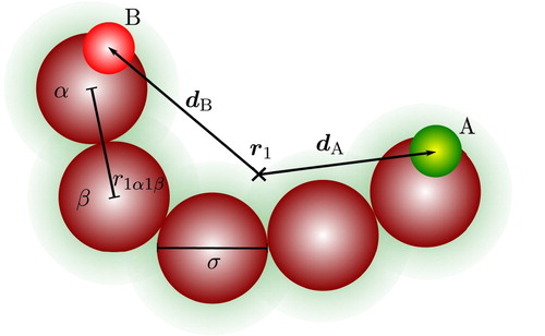
We consider model associating molecules comprising $m\ge 1$ fused spherical segments of diameter σ (noting that m=1 corresponds to a spherical model and m>1 to a chain model), with short-range association sites embedded in the segments to mediate directional interactions of the hydrogen-bonding type (Figure 1). Further details are provided in the following subsections. We consider first the form of the pair potential needed to incorporate intra- as well as intermolecular interactions, impose a set of steric restrictions (following Wertheim's original approach [26,27]), and discuss the types of aggregates resulting.

Figure 1. A two-site associating chain molecule comprising five tangentially bonded spherical segments and two association sites labelled A and B. The position of the centre of mass of the molecule is indicated by ${\mathit{r}}_1$, and the displacement site vectors by ${\mathit{d}}_A$ and ${\mathit{d}}_B$, which are function of the molecular orientation and conformation ${\mathit{\Omega }}_1$. The distance between two segments α and β of the molecule at position ${\mathit{r}}_1$ is represented by $r_{1\alpha 1\beta }$.

2.1. Molecular pair potentials

In order to treat both inter- and intramolecular interactions, two pair potentials are considered: a pair interaction potential ${\varphi }^{\mathrm{inter}}$ between two molecules 1 and 2, and a pair interaction potential ${\varphi }^{\mathrm{intra}}$ between two segments in the same molecule. The intermolecular pair potential is given as the sum of a reference ${\varphi }^{\mathrm{ref}}$and a perturbative association HB potential ${\varphi }_{\mathit{s}{\mathit{s}}^{\prime }}^{\mathrm{HB},\mathrm{inter}}$ [26,54]: (1) $\begin{array}{rl}& {\varphi }^{\mathrm{inter}}({\mathit{r}}_{12},{\mathit{\Omega }}_1,{\mathit{\Omega }}_2)={\varphi }^{\mathrm{ref}}({\mathit{r}}_{12},{\mathit{\Omega }}_1,{\mathit{\Omega }}_2)\\ & +\sum _{s\in \Gamma }\sum _{s^{\prime }\in \Gamma }{\varphi }_{\mathit{s}{\mathit{s}}^{\prime }}^{\mathrm{HB},\mathrm{inter}}({\mathit{r}}_{12},{\mathit{\Omega }}_1,{\mathit{\Omega }}_2),\end{array}$(1) where ${\mathit{r}}_{12}$ represents the vector between the centres of two molecules with centres of mass in positions ${\mathit{r}}_1$ and ${\mathit{r}}_2$, i.e., ${\mathit{r}}_{12}={\mathit{r}}_2-{\mathit{r}}_1$, and ${\mathit{\Omega }}_1$ and ${\mathit{\Omega }}_2$ are vectors containing the respective angles characterising the molecular orientation and conformation, including all angles subtended by the constituting segments and the association sites. The reference intermolecular potential is assumed to be given by a sum of intersegment potentials between the segments that constitute the molecules [70], thus (2) ${\varphi }^{\mathrm{ref}}({\mathit{r}}_{12},{\mathit{\Omega }}_1,{\mathit{\Omega }}_2)=\sum _{\alpha }\sum _{\beta }{\varphi }_{\alpha \beta }^{\mathrm{ref}}(r_{1\alpha 2\beta }),$(2) where $r_{1\alpha 2\beta }$ is the distance between segment α present in molecule 1 and segment β in molecule 2 given by $|({\mathit{r}}_2+{\mathit{d}}_{\beta }({\mathit{\Omega }}_2))-({\mathit{r}}_1+{\mathit{d}}_{\alpha }({\mathit{\Omega }}_1))|$, ${\mathit{d}}_{\beta }$ is the displacement vector of the core of segment β from the centre of the molecule in position ${\mathit{r}}_2$, and ${\mathit{d}}_{\alpha }$ is the displacement vector of the core of segment α from the centre of the molecule in position ${\mathit{r}}_1$ (cf. Section 2.1). Any spherically symmetric potential (hard-sphere, square-well, Mie, Lennard-Jones, …) can be used as ${\varphi }_{\alpha \beta }^{\mathrm{ref}}(r_{1\alpha 2\beta })$.

Short-ranged directional site–site interactions between molecules are promoted through association sites. Segments may contain any number of sites. We use uppercase letters A,B,… to refer to labelled sites, lowercase letters $a,b,\dots$ to refer to association site types, and $s,s^{\prime },\dots$ to refer to sites in general. The interaction between sites $s$ and $s^{\prime }$ in molecules 1 and 2 are modelled using square-well (SW) potentials, so that the intermolecular site–site interaction is given by (3) $\begin{array}{rl}& {\varphi }_{\mathit{s}{\mathit{s}}^{\prime }}^{\mathrm{HB},\mathrm{inter}}({\mathit{r}}_{12},{\mathit{\Omega }}_1,{\mathit{\Omega }}_2)\\ & =\{\begin{array}{ll}-{\epsilon }_{\mathit{a}\mathit{b}}^{\mathrm{HB}}& ,|{\mathit{r}}_{12}+{\mathit{d}}_{s^{\prime }}({\mathit{\Omega }}_2)-{\mathit{d}}_s({\mathit{\Omega }}_1)|<r_{\mathit{a}\mathit{b}}^{\mathrm{c}}\\ 0& ,\mathrm{else}\end{array},\end{array}$(3) where ${\epsilon }_{ab}^{\mathrm{HB}}$ is the well depth of the square-well interaction between sites of types a and b, ${\mathit{d}}_s({\mathit{\Omega }}_1)$ is the displacement vector of site $s$ from the centre of the molecule in position ${\mathit{r}}_1$ (cf. Figure 1), ${\mathit{d}}_{s^{\prime }}({\mathit{\Omega }}_2)$ is the displacement vector of site $s^{\prime }$ from the centre of the molecule in position ${\mathit{r}}_2$, $|{\mathit{r}}_{12}+{\mathit{d}}_{s^{\prime }}({\mathit{\Omega }}_2)-{\mathit{d}}_s({\mathit{\Omega }}_1)|=|({\mathit{r}}_2+{\mathit{d}}_{s^{\prime }}({\mathit{\Omega }}_2))-({\mathit{r}}_1+{\mathit{d}}_s({\mathit{\Omega }}_1))|$ denotes the centre-centre distance between association sites $s$ and $s^{\prime }$ in molecules 1 and 2 at coordinates $({\mathit{r}}_1,{\mathit{\Omega }}_1)$ and $({\mathit{r}}_2,{\mathit{\Omega }}_2)$, respectively, and $r_{\mathit{a}\mathit{b}}^{\mathrm{c}}$ is the range of the association interaction between sites of types a and b.

The intramolecular potential ${\varphi }^{\mathrm{intra}}$ is analogously defined as (4) ${\varphi }^{\mathrm{intra}}({\mathit{\Omega }}_1)={\varphi }^{\mathrm{ref}}({\mathit{\Omega }}_1)+\frac{1}{2}\sum _{s\in \Gamma }\sum _{s^{\prime }\in \Gamma }{\varphi }_{\mathit{s}{\mathit{s}}^{\prime }}^{\mathrm{HB},\mathrm{intra}}({\mathit{\Omega }}_1),$(4) where the distance between segments and sites is given by the orientational/conformational vector ${\mathit{\Omega }}_1$, and the factor 1/2 is included to prevent double counting, since the associating sites of the pair $\mathit{s}{\mathit{s}}^{\prime }$ are located in the same molecule. The reference intramolecular potential is assumed to be given by a sum of intersegmental potentials between the segments that constitute the molecule [70]: (5) ${\varphi }^{\mathrm{ref}}({\mathit{\Omega }}_1)=\frac{1}{2}\sum _{\alpha }\sum _{\beta }{\varphi }_{\alpha \beta }^{\mathrm{ref}}(r_{1\alpha 1\beta }).$(5) The site–site intramolecular interaction is modelled using a SW potential so that, (6) ${\varphi }_{\mathit{s}{\mathit{s}}^{\prime }}^{\mathrm{HB},\mathrm{intra}}({\mathit{\Omega }}_1)=\{\begin{array}{ll}-{\epsilon }_{\mathit{a}\mathit{b}}^{\mathrm{HB}}& |{\mathit{d}}_{s^{\prime }}({\mathit{\Omega }}_1)-{\mathit{d}}_s({\mathit{\Omega }}_1)|<r_{\mathit{a}\mathit{b}}^{\mathrm{c}}\\ 0& \mathrm{else}\end{array},$(6) and the potential is a function of the site–site distance and orientation of sites $s$ and $s^{\prime }$ of a molecule in coordinates ${\mathit{r}}_1$ given by the vector $|{\mathit{d}}_{s^{\prime }}({\mathit{\Omega }}_1)-{\mathit{d}}_s({\mathit{\Omega }}_1)|$. The intramolecular potential is non-zero only for the pair of sites in the molecule that are sterically (site–site distance $<r_{\mathit{a}\mathit{b}}^{\mathrm{c}}$) and energetically (${\epsilon }_{\mathit{a}\mathit{b}}^{\mathrm{HB}}>0$) favourable to association.

2.2. Steric restrictions

Bonding constraints restricting the type of possible site–site interactions, are imposed following those of the original TPT1 approach [26,27] (Figure 2). In the first restriction, when a bond between two sites located in different segments is formed, the repulsive cores of the two segments prevent a third from participating in bonding without the cores overlapping (Figure 2(a)). In the second restriction the angle between any two given sites in a molecule is assumed to be large enough to prevent double (or multiple) bonding between two segments, such that a site may participate in one bond only (Figure 2(b)). Finally, double bonding between any two segments is not permitted (Figure 2(c)).

Figure 2. Constraints of TPT1 [28] restrict the following bonding schemes: (a) the repulsive cores of two associating molecules prevent a third core participating in bonding; (b) a site may participate in one bond only; (c) double-bonding between any two segments is not permitted.

In the molecular model considered no limit is imposed on the number of association sites that are located in a given segment or molecule and the precise positions of the sites in a given segment are not specified. It is however assumed that their configuration is such to conform to the steric incompatibilities described earlier. Accordingly, a one-site molecule leads only to the formation of dimers, while in a two-site molecule linear chain aggregates (dimers, trimers, tetramers,…) as well as rings (of inter- or intramolecularly bonded molecules) of any size may form. Open, linear and branched chains as well as ring aggregates may form in the case of models with three or more association sites (see Figure 3 and 4).

Figure 3. Examples of association aggregates formed in a spherical model fluid of molecules shown in (a) with three association sites (labelled A, B, C). The check marks and crosses indicate whether the aggregate type is accounted for by the theory presented in our current work or not: (a) monomer species; (b) open branched chain; (c) intermolecular ring bonded through A–B bonds only; (d) intermolecular ring bonded through A–B bonds only, with further branching; (e) A–B intermolecular ring associated to a B–C intermolecular ring; and (f) intermolecular ring involving more than one type of site–site interaction.

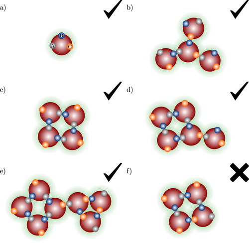
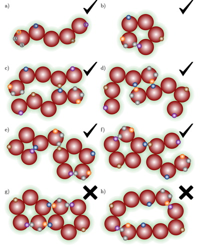
Figure 4. Examples of the association aggregates that can be found in a fluid of chain molecules shown in (a) with multiple association sites, A, B, C,….The check marks and crosses indicate whether the aggregate type is accounted for by the theory presented in our current work or not: (a) monomer species; (b) intramolecular ring; (c) open chain aggregate; (d) intermolecular ring containing only one type of site–site bond (B–C); (e) intramolecular ring with a C–E bond associated to an A–E intramolecular ring; (f) branched A–E intramolecular ring; (g) molecule involved in more than one ring; and (h) ring involving more than one type of site–site interaction.

In the case of the formation of ring-like clusters and intramolecular association, the steric restrictions do not limit the formation of such aggregates. In our framework we account for ring-like structures that are formed by molecules of the same species only and that have a single type of site–site interaction within the ring aggregate; different rings, each including a different type of site–site interaction are, nevertheless allowed. Moreover, ring-ring aggregate formation is also considered. In multi-component systems ring-like aggregates of any of the components of the mixture are taken into account, including larger clusters of rings of different components. Examples of the types of aggregates accounted for in our approach are presented in detail in the following sections.

2.3. Spherical molecules

In a fluid of spherical molecules with two or more association sites, following the previously discussed restrictions, association can result in the formation of open aggregates (linear or branched chains; cf. Figure 3(b)) and intermolecular rings containing three or more molecules; intramolecular bonding and a two-sphere ring, which amounts to double bonding, are not considered. Intermolecular ring-like aggregates may form by association of three or more molecules of a given component involving site–site interactions of only one type, see examples in Figures 3(c–e). Intermolecular rings of arbitrary size may form, and ring—ring association that leads to the formation of larger clusters is also taken into account (cf. Figure 3(e)). Intermolecular ring-like clusters involving more than one type of site–site interaction are however excluded in our framework (cf. Figure 3(f)).

2.4. Chain molecules

In a fluid of chain molecules with m>2 segments (Figure 4), in addition to the types of intermolecular interactions discussed in the previous section, intramolecular site–site interactions are also possible. Examples of the types of possible aggregates in such a fluid are presented in Figure 4. The same restrictions for the formation of intermolecular open clusters and ring-like aggregates as described for the case of spherical molecules apply. Intramolecular association is also possible (i.e. aggregates involving only one molecule; cf. Figure 4(b)), as well as closed aggregates involving only two molecules (cf. Figure 4(d)). In the case of a ring-like aggregate with two molecules, only one type of site–site interaction is allowed within the ring.

3. The Helmholtz free energy

The Helmholtz free energy of a pure associating fluid can be obtained considering molecules in a non-associated monomer, dimer, chain, intermolecular ring of size τ, and intramolecular ring configurations, and any other cluster species that may be present in the fluid as distinct species, so that [55,71] (7) $\begin{array}{rl}A& =N_0{\mu }_0+N_{\mathrm{dimer}}{\mu }_{\mathrm{dimer}}+N_{\mathrm{trimer}}{\mu }_{\mathrm{trimer}}+\cdots \\ & +\sum _{R=1}^{N_{\mathrm{RS}}}{N}_{{\tau }_R}{\mu }_{{\tau }_R}+\cdots +N_{\mathrm{intra}}{\mu }_{\mathrm{intra}}+\cdots -PV,\end{array}$(7) where P is the pressure, V the total volume, μ the chemical potential, and the subscripts refer to the type of species. $N_0$ is the number molecules in a monomer configuration, $N_{\mathrm{dimer}}$ is the number of molecules participating in dimers, $N_{\mathrm{trimer}}$ is the number of molecules participating in aggregates of open chains of three molecules, and so on…., $N_{{\tau }_R}$ is the number of molecules which are intermolecularly bonded into rings of size ${\tau }_R\ge 2$ for chain molecules or ${\tau }_R\ge 3$ for spherical molecules (with ${\tau }_R$ corresponding to the number of molecules in the ring). The summation is over the number of different ring sizes, $N_{\mathrm{RS}}$. Double and larger ring clusters, as well as ring-chain clusters may also form, extending Equation (7). $N_{\mathrm{intra}}$ is the number of molecules with an intramolecular hydrogen bond only; i.e., not participating in any other type of aggregate. Furthermore, and ${\mu }_0$ is the chemical potential of the monomer species, ${\mu }_{\mathrm{dimer}}$ is the chemical potential of the dimers, $N_{\mathrm{trimer}}$ is the chemical potential of the trimers, ${\mu }_{{\tau }_R}$ is the chemical potential of intermolecular rings of size ${\tau }_R$, and ${\mu }_{\mathrm{intra}}$ is the chemical potential of molecules with intramolecular association only. At equilibrium, the chemical potential of all the molecules in the system must be the same regardless of cluster arrangements, including monomers, which allows us to write Equation (7(7) $\begin{array}{rl}A& =N_0{\mu }_0+N_{\mathrm{dimer}}{\mu }_{\mathrm{dimer}}+N_{\mathrm{trimer}}{\mu }_{\mathrm{trimer}}+\cdots \\ & +\sum _{R=1}^{N_{\mathrm{RS}}}{N}_{{\tau }_R}{\mu }_{{\tau }_R}+\cdots +N_{\mathrm{intra}}{\mu }_{\mathrm{intra}}+\cdots -PV,\end{array}$(7) ) as (8) $A=N{\mu }_0-PV,$(8) where the total number of molecules N in the system, regardless of their bonded state, is given by (9) $\begin{array}{rl}N& =N_0+N_{\mathrm{dimer}}+N_{\mathrm{trimer}}+\cdots \\ & +\sum _{R=1}^{N_{\mathrm{RS}}}{N}_{{\tau }_R}+\cdots +N_{\mathrm{intra}}.\end{array}$(9) Following an observation by Andersen [16,17] that the form of the combinatorial terms in the cluster expansion of associated fluids is independent of the density, the Helmholtz free energy can be determined by considering the limit of low density; the results obtained in the low-density limit are also valid at higher densities. It is thus possible to derive an expression for the association term of an ideal associating fluid following Dalton's law, i.e., assuming a proportionality between the pressure and the total number of aggregates [55,59]: (10) $\begin{array}{rl}{N}_{\mathrm{aggregates}}& =N_0+\frac{N_{\mathrm{dimer}}}{2}+\frac{N_{\mathrm{trimer}}}{3}+\cdots \\ & +\sum _{R=1}^{N_{\mathrm{RS}}}\frac{N_{{\tau }_R}}{{\tau }_R}+\cdots +N_{\mathrm{intra}},\end{array}$(10) so that (11) $A_{\mathrm{aggregates}}=N{\mu }_0-N_{\mathrm{aggregates}}kT,$(11) where k is the Boltzmann constant and T the absolute temperature. The ideal chemical potential of the monomer species is given by [72] (12) ${\mu }_0=kT\ln ({\rho }_0{\rm Y}(T)),$(12) where ${\rho }_0=N_0/V$ is the number density of monomers and ${\rm Y}(T)$ is a function of temperature that includes the translational, rotational, and vibrational parts of the molecular partition function (the de Broglie volume) as well as other contributions from molecular configurations [70].

From this analysis it can be seen that the number of aggregates in the system and consequently the expression for the Helmholtz free energy directly depend on the type of species considered. We start by considering the simplest case of a non-associating fluid then proceed to incorporate association.

3.1. Non-associating monomers

In a non-associating system the only species present is the monomer, so that, $N_{\mathrm{aggregates}}=N_0=N$ and the number density ($\rho =N/V$) is equal to the density of monomers; i.e., ${\rho }_0=\rho$. It therefore follows from Equations (11(11) $A_{\mathrm{aggregates}}=N{\mu }_0-N_{\mathrm{aggregates}}kT,$(11) ) and (12(12) ${\mu }_0=kT\ln ({\rho }_0{\rm Y}(T)),$(12) ) that the free energy in a non-associating ideal system $A_0$ can be written in terms of the number density of the system as (13) $A_0=NkT[\ln (\rho {\rm Y}(T))-1],$(13) which corresponds to an ideal gas [72].

3.2. Free monomers and open-chain aggregates

We consider a system at fixed V, T containing ten molecules; if two molecules associate to form a dimer, nine aggregates remain, if further association occurs with another molecule to form a trimer, $N_{\mathrm{aggregates}}=8$ and so on. In the general case, the number of aggregates in a fluid where the molecules associate only in chains (branching is possible but not ring formation) is reduced by one per association bond formed. It is helpful to define at this point the fraction of molecules with sites in set $\alpha \subseteq \Gamma$ free as $X_{\alpha }$. Note that the molecules that contribute to $X_{\alpha }$ have all sites in α free at least, but not exclusively (other sites might be free). In this notation, $X_{\Gamma }$ corresponds to the fraction of molecules with all sites free, i.e., the fraction of free monomer molecules. Traditionally this fraction is referred to as $X_0$ [30]; we follow this convention hereafter¹. The fraction of molecules with (at least) site $s$ free is given by $X_{\{s\}}$, often referred to as $X_s$, and the fraction of molecules with $s$ bonded is then given by $(1-X_s)$. This means that for a model with the set of sites Γ, the number of aggregates can be obtained as (14) $N_{\mathrm{aggregates}}=N-\frac{1}{2}N\sum _{s\in \Gamma }(1-X_s),$(14) where the factor 1/2 is included to avoid double counting the number of bonds, as each bond involves two sites. The corresponding form of the Helmholtz free energy is thus given by (15) $A=NkT[\ln ({\rho }_0{\rm Y}(T))-1+\frac{1}{2}\sum _{s\in \Gamma }(1-X_s)].$(15)

3.3. Free monomers, open chains, and intramolecular ring-like aggregates

A system in which intramolecular association is taken into account in addition to the formation of intermolecular chain-like aggregates is now considered. The formation of an intramolecular bond does not change the number of aggregates in the system but, by competing with the formation of intermolecular bonds, it will affect the overall free energy of the system. To avoid confusion, we introduce $X_s^{\mathrm{open}}$ as the fraction of molecules with site $s$ not bonded in an open chain, and re-express Equation (14(14) $N_{\mathrm{aggregates}}=N-\frac{1}{2}N\sum _{s\in \Gamma }(1-X_s),$(14) ) for the total number of aggregates as [55] (16) $N_{\mathrm{aggregates}}=N-\frac{1}{2}N\sum _{s\in \Gamma }(1-X_s^{\mathrm{open}}),$(16) and the Helmholtz free energy as (17) $A=NkT[\ln ({\rho }_0{\rm Y}(T))-1+\frac{1}{2}\sum _{s\in \Gamma }(1-X_s^{\mathrm{open}})].$(17) One should also note that the sum of the fraction of molecules with site $s$ bonded in open chains and the fraction of molecules with site $s$ bonded in intramolecular rings $(1-X_s^{\mathrm{intra}})$ corresponds to the total fraction of molecules with site $s$ bonded $(1-X_s)$. Therefore, for a given site $s$ a relation (18) $(1-X_s^{\mathrm{open}})+(1-X_s^{\mathrm{intra}})=1-X_s,$(18) can be written, which can be substituted in Equation (17(17) $A=NkT[\ln ({\rho }_0{\rm Y}(T))-1+\frac{1}{2}\sum _{s\in \Gamma }(1-X_s^{\mathrm{open}})].$(17) ) so that, (19) $\begin{array}{rl}A& =NkT[\ln ({\rho }_0{\rm Y}(T))-1+\frac{1}{2}\sum _{s\in \Gamma }(1-X_s)\\ & -\frac{1}{2}\sum _{s\in \Gamma }(1-X_s^{\mathrm{intra}})].\end{array}$(19) The last term in this expression corresponds to the fraction of molecules forming intramolecular rings ${\xi }_1$: (20) ${\xi }_1=\frac{1}{2}\sum _{s\in \Gamma }(1-X_s^{\mathrm{intra}}),$(20) where we use the subscript 1 to indicate a ring-like aggregate involving one molecule only.

3.4. Free monomers, open chains, and intra- and intermolecular ring-like aggregates

The formation of each intermolecular ring cluster involving τ molecules reduces the number of free aggregates in the system by $\tau -1$. Accounting for this, the number of aggregates in the system is now given by (21) $\begin{array}{rl}{N}_{\mathrm{aggregates}}& =N-\frac{1}{2}N\sum _{s\in \Gamma }(1-X_s^{\mathrm{open}})\\ & -\sum _{R=1}^{N_{\mathrm{RS}}}({\tau }_R-1)\times N_{{\tau }_R}/{\tau }_R,\end{array}$(21) where $N_{{\tau }_R}$ is the number of molecules in rings of size ${\tau }_R\ge 1$, which can be obtained in terms of the fraction of molecules involved in ring formation ${\xi }_{{\tau }_R}$ as (22) $N_{{\tau }_R}={\xi }_{{\tau }_R}N.$(22) It is also possible to write ${\xi }_{{\tau }_R}$ in terms of the fraction of molecules with a ring-bonding site $s$ free $X_s^{\mathrm{rings}{\tau }_R}$ as (23) ${\xi }_{{\tau }_R}=\frac{1}{2}\sum _{s\in \Gamma }(1-X_s^{\mathrm{rings}{\tau }_R}),$(23) noting that in the case of ${\tau }_R=1$, ${\xi }_{{\tau }_R}={\xi }_1$ and $X_s^{\mathrm{rings}{\tau }_R}=X_s^{\mathrm{intra}}$. Substituting Equations (22(22) $N_{{\tau }_R}={\xi }_{{\tau }_R}N.$(22) ) and (23(23) ${\xi }_{{\tau }_R}=\frac{1}{2}\sum _{s\in \Gamma }(1-X_s^{\mathrm{rings}{\tau }_R}),$(23) ) in (21(21) $\begin{array}{rl}{N}_{\mathrm{aggregates}}& =N-\frac{1}{2}N\sum _{s\in \Gamma }(1-X_s^{\mathrm{open}})\\ & -\sum _{R=1}^{N_{\mathrm{RS}}}({\tau }_R-1)\times N_{{\tau }_R}/{\tau }_R,\end{array}$(21) ) allows one to rewrite the number of aggregates in the system as (24) $\begin{array}{rl}{N}_{\mathrm{aggregates}}& =N[1-\frac{1}{2}\sum _{s\in \Gamma }(1-X_s^{\mathrm{open}})\\ & -\sum _{R=1}^{N_{\mathrm{RS}}}\frac{({\tau }_R-1)}{{\tau }_R}\times \frac{1}{2}\sum _{s\in \Gamma }(1-X_s^{\mathrm{rings}{\tau }_R})].\end{array}$(24) Analogously to Equation (18(18) $(1-X_s^{\mathrm{open}})+(1-X_s^{\mathrm{intra}})=1-X_s,$(18) ), the relation (25) $(1-X_s^{\mathrm{open}})+\sum _{R=1}^{N_{\mathrm{RS}}}(1-X_s^{\mathrm{rings}{\tau }_R})=1-X_s,$(25) holds and, upon insertion in Equation (24(24) $\begin{array}{rl}{N}_{\mathrm{aggregates}}& =N[1-\frac{1}{2}\sum _{s\in \Gamma }(1-X_s^{\mathrm{open}})\\ & -\sum _{R=1}^{N_{\mathrm{RS}}}\frac{({\tau }_R-1)}{{\tau }_R}\times \frac{1}{2}\sum _{s\in \Gamma }(1-X_s^{\mathrm{rings}{\tau }_R})].\end{array}$(24) ), the number of aggregates is simply given by (26) $N_{\mathrm{aggregates}}=N[1-\frac{1}{2}\sum _{s\in \Gamma }(1-X_s)+\sum _{R=1}^{N_{\mathrm{RS}}}\frac{1}{{\tau }_R}\times {\xi }_{{\tau }_R}],$(26) which can be used to write the total Helmholtz free energy of a fluid comprising open and ring-like aggregates (in the low-density limit) as (27) $\begin{array}{rl}A& =NkT[\ln ({\rho }_0{\rm Y}(T))-1+\frac{1}{2}\sum _{s\in \Gamma }(1-X_s)\\ & -\sum _{R=1}^{N_{\mathrm{RS}}}\frac{1}{{\tau }_R}{\xi }_{{\tau }_R}].\end{array}$(27) Equation (27(27) $\begin{array}{rl}A& =NkT[\ln ({\rho }_0{\rm Y}(T))-1+\frac{1}{2}\sum _{s\in \Gamma }(1-X_s)\\ & -\sum _{R=1}^{N_{\mathrm{RS}}}\frac{1}{{\tau }_R}{\xi }_{{\tau }_R}].\end{array}$(27) ) provides a way to calculate the total Helmholtz free energy with the proviso that the fractions of molecules in different bonded states $X_0$ (fraction of monomers), $X_{\alpha },\alpha \subseteq \Gamma$, and the fraction ${\xi }_{{\tau }_R}$ of molecules involved in clusters in rings of size ${\tau }_R$ are known at a specified thermodynamic state N,V,T. In order to derive expressions for these distributions of molecular bonded states we make use of Wertheim's TPT1 [28,73], extending the framework to account for ring formation.

4. Mass action equations

Wertheim introduced the multi-density concept, which translates into treating molecules in different bonding states as different pseudo-species, mirroring the framework presented in Section 3. In his formalism, a density ${\rho }_s$ is associated with molecules with site $s$ bonded, a density ${\rho }_{\mathit{s}{\mathit{s}}^{\prime }}$ to molecules with sites $s$ and $s^{\prime }$ bonded, and so on. More generally, the number density of molecules with sites in the set α bonded is ${\rho }_{\alpha }$, where α is a subset of the set of all sites Γ, including the empty set $\mathrm{\varnothing }$ that conventionally corresponds to the density of molecules not bonded (${\rho }_{\alpha }={\rho }_0,\mathrm{for}\alpha =\mathrm{\varnothing }$). Following Sear and Jackson [74], we present expressions considering an inhomogeneous system first, in which the densities are dependent on position coordinates $\mathit{r}$ and the orientation and conformation vector $\mathit{\Omega }$, and we make use of $(1)$ as short-hand notation for $({\mathit{r}}_1,{\mathit{\Omega }}_1)$ which refers to all degrees of freedom of molecule 1.

The local number density $\rho (1)$ of particles in coordinates $(1)$ $(\int \rho (1)\mathrm{d}(1)=N)$ can be written as the sum of all bonding-state densities as [28] (28) $\rho (1)=\sum _{\alpha \subseteq \Gamma }{\rho }_{\alpha }(1).$(28) Furthermore, Wertheim [28] defined ${\sigma }_{\alpha }(1)$ as the density of molecules that are not bonded plus the ones that are bonded exactly through one, some or all sites in the set α. Accordingly, ${\sigma }_{\Gamma -\alpha }(1)$ is the density of molecules with (at least) the sites in the set α free. As an example, in a two-site model with sites A and B, i.e., $\Gamma =\{A,B\}$, ${\sigma }_{\Gamma -A}(1)={\sigma }_B(1)$ is the density of molecules with site B free, and is given by the sum ${\rho }_0(1)+{\rho }_B(1)$. More generally, (29) ${\sigma }_{\alpha }(1)=\sum _{\delta \subseteq \alpha }{\rho }_{\delta }(1),$(29) with the special cases ${\sigma }_0(1)={\rho }_0(1)$ (the density of monomers) and ${\sigma }_{\Gamma }(1)=\rho (1)$ the total number density of molecules in the system, regardless of their bonded state (given by N/V, cf., Equation (9(9) $\begin{array}{rl}N& =N_0+N_{\mathrm{dimer}}+N_{\mathrm{trimer}}+\cdots \\ & +\sum _{R=1}^{N_{\mathrm{RS}}}{N}_{{\tau }_R}+\cdots +N_{\mathrm{intra}}.\end{array}$(9) )). The density of molecules with sites in set α free is related to the fraction of molecules with set of sites α free by (30) ${\sigma }_{\Gamma -\alpha }(1)=\rho (1)X_{\alpha }(1),\mathrm{\forall }\alpha \subset \Gamma ,$(30) and to the fraction of monomers (31) ${\sigma }_{\Gamma -\alpha }(1)={\rho }_0(1)=\rho (1)X_0(1),$(31) for $\alpha =\Gamma$.

In Wertheim's work [28,29] the Helmholtz free energy expression is expressed as (32) $\begin{array}{rl}{A}_{\mathrm{Wert}}[\{\rho \}]& =kT\int [\rho (1)\ln \left(\frac{{\rho }_0(1)}{\rho (1)}\right)\\ & +\rho (1)+Q(1)\phantom{\rho (1)\ln \left(\frac{{\rho }_0(1)}{\rho (1)}\right)}]\mathrm{d}(1)-kT\mathrm{\Delta }{c}^{(0)}[\{\rho \}],\end{array}$(32) where the notation $\{\rho \}=\{{\rho }_0,{\rho }_A,\dots \}$ highlights the dependence of the free energy on all bonding state densities. Following Wertheim's formalism, each density ${\rho }_{\alpha }$ is defined in terms of a sum of graphs². $A_{\mathrm{Wert}}$ corresponds to the difference in free energy between the associating system and a reference (non-associating) system, (33) $A_{\mathrm{Wert}}=A-A_{\mathrm{ref}},$(33) where all interactions other than association are accounted for in the reference fluid, including chain connectivity in the case of chain-like molecules as well any repulsive and dispersion interactions included in the model.

Equation (32(32) $\begin{array}{rl}{A}_{\mathrm{Wert}}[\{\rho \}]& =kT\int [\rho (1)\ln \left(\frac{{\rho }_0(1)}{\rho (1)}\right)\\ & +\rho (1)+Q(1)\phantom{\rho (1)\ln \left(\frac{{\rho }_0(1)}{\rho (1)}\right)}]\mathrm{d}(1)-kT\mathrm{\Delta }{c}^{(0)}[\{\rho \}],\end{array}$(32) ) is a general expression that incorporates all possible aggregates (i.e., inter- and intramolecular rings as well as open chain aggregates); it provides a different route to express the association contribution to the free energy given by Equation (27(27) $\begin{array}{rl}A& =NkT[\ln ({\rho }_0{\rm Y}(T))-1+\frac{1}{2}\sum _{s\in \Gamma }(1-X_s)\\ & -\sum _{R=1}^{N_{\mathrm{RS}}}\frac{1}{{\tau }_R}{\xi }_{{\tau }_R}].\end{array}$(27) ). The difference between the two equations is that Equation (32(32) $\begin{array}{rl}{A}_{\mathrm{Wert}}[\{\rho \}]& =kT\int [\rho (1)\ln \left(\frac{{\rho }_0(1)}{\rho (1)}\right)\\ & +\rho (1)+Q(1)\phantom{\rho (1)\ln \left(\frac{{\rho }_0(1)}{\rho (1)}\right)}]\mathrm{d}(1)-kT\mathrm{\Delta }{c}^{(0)}[\{\rho \}],\end{array}$(32) ) is a general expression, before equilibrium is imposed, that reduces to Equation (27(27) $\begin{array}{rl}A& =NkT[\ln ({\rho }_0{\rm Y}(T))-1+\frac{1}{2}\sum _{s\in \Gamma }(1-X_s)\\ & -\sum _{R=1}^{N_{\mathrm{RS}}}\frac{1}{{\tau }_R}{\xi }_{{\tau }_R}].\end{array}$(27) ) at equilibrium and after including the ideal contribution. As such, the mass action equations for the distribution of bonding states needed in Equation (27(27) $\begin{array}{rl}A& =NkT[\ln ({\rho }_0{\rm Y}(T))-1+\frac{1}{2}\sum _{s\in \Gamma }(1-X_s)\\ & -\sum _{R=1}^{N_{\mathrm{RS}}}\frac{1}{{\tau }_R}{\xi }_{{\tau }_R}].\end{array}$(27) ) can be obtained by minimisation of the free energy given by Equation (32(32) $\begin{array}{rl}{A}_{\mathrm{Wert}}[\{\rho \}]& =kT\int [\rho (1)\ln \left(\frac{{\rho }_0(1)}{\rho (1)}\right)\\ & +\rho (1)+Q(1)\phantom{\rho (1)\ln \left(\frac{{\rho }_0(1)}{\rho (1)}\right)}]\mathrm{d}(1)-kT\mathrm{\Delta }{c}^{(0)}[\{\rho \}],\end{array}$(32) ) [26,28,52].

The function Q in Equation (32(32) $\begin{array}{rl}{A}_{\mathrm{Wert}}[\{\rho \}]& =kT\int [\rho (1)\ln \left(\frac{{\rho }_0(1)}{\rho (1)}\right)\\ & +\rho (1)+Q(1)\phantom{\rho (1)\ln \left(\frac{{\rho }_0(1)}{\rho (1)}\right)}]\mathrm{d}(1)-kT\mathrm{\Delta }{c}^{(0)}[\{\rho \}],\end{array}$(32) ) results from the nontrivial derivation originally presented by Wertheim [28] and recently re-derived in an excellent review by Zmpitas and Gross [73]. It is given by (34) $\begin{array}{rl}Q(1)& =-\sum _{s\in \Gamma }{\sigma }_{\Gamma -s}(1)+{\rho }_0(1)\\ & \times \sum _{\begin{array}{c}\{{\gamma }_1,\dots {\gamma }_M\}\\ \in \mathcal{P}(\Gamma ),M\ge 2\end{array}}(-1{)}^M(M-2)!\prod _{i=1}^M\frac{{\sigma }_{{\gamma }_i}(1)}{{\rho }_0(1)},\end{array}$(34) where the first sum is over all sites and the second over all possible partitions of the set ($\mathcal{P}(\Gamma )$), i.e., the possible ways to divide Γ into pairwise disjoint subsets. The elements of the partition of Γ into M subsets are ${\gamma }_1,{\gamma }_2,\dots ,{\gamma }_M$ and the condition $M\ge 2$ ensures that each partition considered must contain two or more elements [28].

The functional $\mathrm{\Delta }{c}^{(0)}=c^{(0)}-c_{\mathrm{ref}}^{(0)}$ in Equation (32(32) $\begin{array}{rl}{A}_{\mathrm{Wert}}[\{\rho \}]& =kT\int [\rho (1)\ln \left(\frac{{\rho }_0(1)}{\rho (1)}\right)\\ & +\rho (1)+Q(1)\phantom{\rho (1)\ln \left(\frac{{\rho }_0(1)}{\rho (1)}\right)}]\mathrm{d}(1)-kT\mathrm{\Delta }{c}^{(0)}[\{\rho \}],\end{array}$(32) ) is referred to by Wertheim [28] as the fundamental graph sum, where $c^{(0)}$ is the correction quantity to the free energy due to cluster-forming interactions, while $c_{\mathrm{ref}}^{(0)}$ is the contribution from interactions existing in the reference fluid. While Q remains unchanged regardless of the types of association clusters considered, $\mathrm{\Delta }{c}^{(0)}$ is dependent on these. In the following section we study in detail the different contributions in this term.

4.1. The fundamental graph sum $\mathrm{\Delta }{c}^{(0)}$

The fundamental graph sum $\mathrm{\Delta }{c}^{(0)}$ relates the possible bonded states of the molecular model to the number of species in the system $N_{\mathrm{species}}$ (cf. Equation (10(10) $\begin{array}{rl}{N}_{\mathrm{aggregates}}& =N_0+\frac{N_{\mathrm{dimer}}}{2}+\frac{N_{\mathrm{trimer}}}{3}+\cdots \\ & +\sum _{R=1}^{N_{\mathrm{RS}}}\frac{N_{{\tau }_R}}{{\tau }_R}+\cdots +N_{\mathrm{intra}},\end{array}$(10) )). It includes all irreducible graphs responsible for the different aggregates. Graphs corresponding to open-chain aggregates can be topologically reduced [29,72] to graphs containing an association bond between pairs of particles (dimers), while ring graphs are irreducible and cannot therefore be accounted for by the same graphs corresponding to open chains [52,62]. Here, we consider open-chain ($\mathrm{\Delta }{c}_{\mathrm{open}}^{(0)}$), intermolecular ring ($\mathrm{\Delta }{c}_{\mathrm{inter}\mathrm{ring}}^{(0)}$), and intramolecular association ($\mathrm{\Delta }{c}_{\mathrm{intra}}^{(0)}$) contributions separately: (35) $\begin{array}{rl}\mathrm{\Delta }{c}^{(0)}[\{\rho \}]& =\mathrm{\Delta }{c}_{\mathrm{open}}^{(0)}[\{\rho \}]\\ & +\mathrm{\Delta }{c}_{\mathrm{inter}\mathrm{ring}}^{(0)}[\{\rho \}]+\mathrm{\Delta }{c}_{\mathrm{intra}}^{(0)}[\{\rho \}].\end{array}$(35)

4.1.1. Open chain-like aggregates

The graph sum for open-chain aggregates $\mathrm{\Delta }{c}_{\mathrm{open}}^{(0)}[\{\rho \}]$ can be expressed as [40] (36) $\begin{array}{rl}& \mathrm{\Delta }{c}_{\mathrm{open}}^{(0)}[\{\rho \}]\\ & =\frac{1}{2}\sum _{s\in \Gamma }\sum _{s^{\prime }\in \Gamma }\int {\sigma }_{\Gamma -s}(1){\sigma }_{\Gamma -s^{\prime }}(2)g_{\mathrm{ref}}({\mathit{r}}_{12},{\mathit{\Omega }}_1,{\mathit{\Omega }}_2)\\ & \times f_{\mathit{s}{\mathit{s}}^{\prime }}({\mathit{r}}_{12},{\mathit{\Omega }}_1,{\mathit{\Omega }}_2)\mathrm{d}(1)\mathrm{d}(2),\end{array}$(36) and accounts for the formation of open chain aggregates of any size. This equation is equivalent to the standard $\mathrm{\Delta }{c}^{(0)}[\{\rho \}]$ of TPT1 [40] for the case when ${\sigma }_{\alpha }$ is defined in terms of segments, i.e., if ${\sigma }_{\Gamma -s}(1)$ is defined as the singlet number density of segments (or spherical molecules) in coordinates (1) with site $s$ free. Our model molecule may, more generally, be non-spherical, instead consisting of an arbitrary number of segments. The graph sum corresponding to Equation (36(36) $\begin{array}{rl}& \mathrm{\Delta }{c}_{\mathrm{open}}^{(0)}[\{\rho \}]\\ & =\frac{1}{2}\sum _{s\in \Gamma }\sum _{s^{\prime }\in \Gamma }\int {\sigma }_{\Gamma -s}(1){\sigma }_{\Gamma -s^{\prime }}(2)g_{\mathrm{ref}}({\mathit{r}}_{12},{\mathit{\Omega }}_1,{\mathit{\Omega }}_2)\\ & \times f_{\mathit{s}{\mathit{s}}^{\prime }}({\mathit{r}}_{12},{\mathit{\Omega }}_1,{\mathit{\Omega }}_2)\mathrm{d}(1)\mathrm{d}(2),\end{array}$(36) ) thus differs from the one used by Wertheim [40] in the sense that it involves molecular graphs, simplifying the analysis; this concept was employed by Marshall and Chapman [75] who showed the relation between segment-based and molecular graphs.

It is possible to interpret Equation (36(36) $\begin{array}{rl}& \mathrm{\Delta }{c}_{\mathrm{open}}^{(0)}[\{\rho \}]\\ & =\frac{1}{2}\sum _{s\in \Gamma }\sum _{s^{\prime }\in \Gamma }\int {\sigma }_{\Gamma -s}(1){\sigma }_{\Gamma -s^{\prime }}(2)g_{\mathrm{ref}}({\mathit{r}}_{12},{\mathit{\Omega }}_1,{\mathit{\Omega }}_2)\\ & \times f_{\mathit{s}{\mathit{s}}^{\prime }}({\mathit{r}}_{12},{\mathit{\Omega }}_1,{\mathit{\Omega }}_2)\mathrm{d}(1)\mathrm{d}(2),\end{array}$(36) ) by physically considering that the formation of an association bond between sites $s$ in molecule 1 and $s^{\prime }$ in molecule 2 is a function of the number densities of molecules with sites $s$ and $s^{\prime }$ free, ${\sigma }_{\Gamma -s}$ and ${\sigma }_{\Gamma -s^{\prime }}$, respectively, and the likelihood of these sites forming a bond, given by the product of the radial distribution of the reference (unbonded) fluid $g_{\mathrm{ref}}$ and the Mayer f-function of the $\mathit{s}{\mathit{s}}^{\prime }$ interaction, in this case, $f_{\mathit{s}{\mathit{s}}^{\prime }}({\mathit{r}}_{12},{\mathit{\Omega }}_1,{\mathit{\Omega }}_2)=\exp (-\beta {\varphi }_{\mathit{s}{\mathit{s}}^{\prime }}^{\mathrm{HB},\mathrm{inter}}({\mathit{r}}_{12},{\mathit{\Omega }}_1,{\mathit{\Omega }}_2))-1$. Molecules interact across all volume and configurations, and therefore their coordinates are integrated over all space and orientations. A sum over all sites $s$ and $s^{\prime }$ is carried out and a factor of one half is included to avoid counting the same pair of sites twice. Any pair of sites is allowed to associate provided that the respective ${\epsilon }_{ab}^{\mathrm{HB}}$ is larger than zero.

4.1.2. Intermolecular ring aggregates

The intermolecular ring contribution from clusters of the types represented in Figures 3(c–e) and 4(d), can be written as [76] (37) $\begin{array}{rl}& \mathrm{\Delta }{c}_{\mathrm{inter}\mathrm{ring}}^{(0)}[\{\rho \}]=\frac{1}{2}\sum _{s\in \Gamma }\sum _{s^{\prime }\in \Gamma -s}\sum _{R=1}^{N_{\mathrm{RS},\mathit{s}{\mathit{s}}^{\prime }}}\frac{1}{{\tau }_R}\\ & \times \int \prod _{i=1}^{{\tau }_R}[g_{\mathrm{ref}}({\mathit{r}}_{i,i+1},{\mathit{\Omega }}_i,{\mathit{\Omega }}_{i+1})f_{\mathit{s}{\mathit{s}}^{\prime }}({\mathit{r}}_{i,i+1},{\mathit{\Omega }}_i,{\mathit{\Omega }}_{i+1})]\\ & \times \prod _{j=1}^{{\tau }_R}{\sigma }_{\Gamma -\mathit{s}{\mathit{s}}^{\prime }}(j)\mathrm{d}(j),\end{array}$(37) generalising the expression provided in reference [53] to an arbitrary number of ring-forming sites, and where the number of molecules per intermolecular ring ${\tau }_R\ge 2,\mathrm{\forall }R$. The density of molecules with both sites $s$ and $s^{\prime }$ free, ${\sigma }_{\Gamma -\mathit{s}{\mathit{s}}^{\prime }}$, is required to model the extent of rings formed, hence the summations in Equation (37(37) $\begin{array}{rl}& \mathrm{\Delta }{c}_{\mathrm{inter}\mathrm{ring}}^{(0)}[\{\rho \}]=\frac{1}{2}\sum _{s\in \Gamma }\sum _{s^{\prime }\in \Gamma -s}\sum _{R=1}^{N_{\mathrm{RS},\mathit{s}{\mathit{s}}^{\prime }}}\frac{1}{{\tau }_R}\\ & \times \int \prod _{i=1}^{{\tau }_R}[g_{\mathrm{ref}}({\mathit{r}}_{i,i+1},{\mathit{\Omega }}_i,{\mathit{\Omega }}_{i+1})f_{\mathit{s}{\mathit{s}}^{\prime }}({\mathit{r}}_{i,i+1},{\mathit{\Omega }}_i,{\mathit{\Omega }}_{i+1})]\\ & \times \prod _{j=1}^{{\tau }_R}{\sigma }_{\Gamma -\mathit{s}{\mathit{s}}^{\prime }}(j)\mathrm{d}(j),\end{array}$(37) ) are over sites $s$ and $s^{\prime }$, with $s\ne s^{\prime }$. This differs from Equation (36(36) $\begin{array}{rl}& \mathrm{\Delta }{c}_{\mathrm{open}}^{(0)}[\{\rho \}]\\ & =\frac{1}{2}\sum _{s\in \Gamma }\sum _{s^{\prime }\in \Gamma }\int {\sigma }_{\Gamma -s}(1){\sigma }_{\Gamma -s^{\prime }}(2)g_{\mathrm{ref}}({\mathit{r}}_{12},{\mathit{\Omega }}_1,{\mathit{\Omega }}_2)\\ & \times f_{\mathit{s}{\mathit{s}}^{\prime }}({\mathit{r}}_{12},{\mathit{\Omega }}_1,{\mathit{\Omega }}_2)\mathrm{d}(1)\mathrm{d}(2),\end{array}$(36) ) where association requires only one site per molecule to be free (${\sigma }_{\Gamma -s}$), where $s$ and $s^{\prime }$ may be the same site (in a different molecule).

In a ring aggregate we consider each molecule in the ring to be close to contact³ with their immediately-neighbouring molecules only. Accordingly, in Equation (37(37) $\begin{array}{rl}& \mathrm{\Delta }{c}_{\mathrm{inter}\mathrm{ring}}^{(0)}[\{\rho \}]=\frac{1}{2}\sum _{s\in \Gamma }\sum _{s^{\prime }\in \Gamma -s}\sum _{R=1}^{N_{\mathrm{RS},\mathit{s}{\mathit{s}}^{\prime }}}\frac{1}{{\tau }_R}\\ & \times \int \prod _{i=1}^{{\tau }_R}[g_{\mathrm{ref}}({\mathit{r}}_{i,i+1},{\mathit{\Omega }}_i,{\mathit{\Omega }}_{i+1})f_{\mathit{s}{\mathit{s}}^{\prime }}({\mathit{r}}_{i,i+1},{\mathit{\Omega }}_i,{\mathit{\Omega }}_{i+1})]\\ & \times \prod _{j=1}^{{\tau }_R}{\sigma }_{\Gamma -\mathit{s}{\mathit{s}}^{\prime }}(j)\mathrm{d}(j),\end{array}$(37) ) we have followed the approximation of Sear and Jackson [74] for the ${\tau }_R$-body distribution function, which is given in terms of pair distribution functions, one per pair of sites, so that (38) $g^{({\tau }_R)}(12\dots {\tau }_R)=\prod _{i=1}^{{\tau }_R}g({\mathit{r}}_{i,i+1},{\mathit{\Omega }}_i,{\mathit{\Omega }}_{i+1}),$(38) where the convention $(i+1)=1$, for $i={\tau }_R$ is used.

The analysis of the expression for $\mathrm{\Delta }{c}_{\mathrm{inter}\mathrm{ring}}^{(0)}[\{\rho \}]$ follows the same rationale as for $\mathrm{\Delta }{c}_{\mathrm{open}}^{(0)}[\{\rho \}]$: in order for an intermolecular ring of size ${\tau }_R$ to form, the molecules must come close enough to form ${\tau }_R$ links between them. It is thus required that sites a and b in each molecule involved are free, correctly oriented and that their interaction energy parameter ${\epsilon }_{ab}^{\mathrm{HB}}$ is larger than zero. As rings of different sizes may form, a sum over the ring size R index is carried out and a factor $1/{\tau }_R$ is introduced to avoid multiple counting. The last bond, $g_{\mathrm{ref}}({\mathit{r}}_{\tau ,1},{\mathit{\Omega }}_{\tau },{\mathit{\Omega }}_1)f_{ab}({\mathit{r}}_{\tau ,1},{\mathit{\Omega }}_{\tau },{\mathit{\Omega }}_1)$ is treated as of a different nature considering its formation to turn an open-chain cluster into a ring. The expression presented in Equation (37(37) $\begin{array}{rl}& \mathrm{\Delta }{c}_{\mathrm{inter}\mathrm{ring}}^{(0)}[\{\rho \}]=\frac{1}{2}\sum _{s\in \Gamma }\sum _{s^{\prime }\in \Gamma -s}\sum _{R=1}^{N_{\mathrm{RS},\mathit{s}{\mathit{s}}^{\prime }}}\frac{1}{{\tau }_R}\\ & \times \int \prod _{i=1}^{{\tau }_R}[g_{\mathrm{ref}}({\mathit{r}}_{i,i+1},{\mathit{\Omega }}_i,{\mathit{\Omega }}_{i+1})f_{\mathit{s}{\mathit{s}}^{\prime }}({\mathit{r}}_{i,i+1},{\mathit{\Omega }}_i,{\mathit{\Omega }}_{i+1})]\\ & \times \prod _{j=1}^{{\tau }_R}{\sigma }_{\Gamma -\mathit{s}{\mathit{s}}^{\prime }}(j)\mathrm{d}(j),\end{array}$(37) ) ensures that a given intermolecular ring is composed by molecules bonded through site–site interactions of only one type. Ring aggregates and structures involving more than one type of site–site interaction (see Figure 3(f) and Figure 4(g,h)) can be accounted for in Equation (37(37) $\begin{array}{rl}& \mathrm{\Delta }{c}_{\mathrm{inter}\mathrm{ring}}^{(0)}[\{\rho \}]=\frac{1}{2}\sum _{s\in \Gamma }\sum _{s^{\prime }\in \Gamma -s}\sum _{R=1}^{N_{\mathrm{RS},\mathit{s}{\mathit{s}}^{\prime }}}\frac{1}{{\tau }_R}\\ & \times \int \prod _{i=1}^{{\tau }_R}[g_{\mathrm{ref}}({\mathit{r}}_{i,i+1},{\mathit{\Omega }}_i,{\mathit{\Omega }}_{i+1})f_{\mathit{s}{\mathit{s}}^{\prime }}({\mathit{r}}_{i,i+1},{\mathit{\Omega }}_i,{\mathit{\Omega }}_{i+1})]\\ & \times \prod _{j=1}^{{\tau }_R}{\sigma }_{\Gamma -\mathit{s}{\mathit{s}}^{\prime }}(j)\mathrm{d}(j),\end{array}$(37) ) by incorporating the relevant Mayer f-functions and densities, but have not been considered in our current work.

4.1.3. Intramolecular association

The intramolecular association contribution from clusters of the types represented in Figures 4(b,e,f), is given by [76] (39) $\begin{array}{rl}& \mathrm{\Delta }{c}_{\mathrm{intra}}^{(0)}[\{\rho \}]\\ & =\frac{1}{2}\sum _{s\in \Gamma }\sum _{s^{\prime }\in \Gamma -s}\int g_{\mathrm{ref}}^{\mathrm{intra}}({\mathit{\Omega }}_1)f_{\mathit{s}{\mathit{s}}^{\prime }}^{\mathrm{intra}}({\mathit{\Omega }}_1){\sigma }_{\Gamma -\mathit{s}{\mathit{s}}^{\prime }}(1)\mathrm{d}(1),\end{array}$(39) where $g_{\mathrm{ref}}^{\mathrm{intra}}({\mathit{\Omega }}_1)$ is the reference intramolecular distribution function, and $f_{\mathit{s}{\mathit{s}}^{\prime }}^{\mathrm{intra}}({\mathit{\Omega }}_1)=\exp (-\beta {\varphi }_{\mathit{s}{\mathit{s}}^{\prime }}^{\mathrm{HB},\mathrm{intra}}({\mathit{\Omega }}_1))-1$. The intramolecular distribution function contains information on the likelihood of any two site-containing segments in a given molecule being at a close distance enough to bond. Additionally the number density of molecules of coordinates (1) with sites $s$ and $s^{\prime }$ simultaneously free, ${\sigma }_{\Gamma -\mathit{s}{\mathit{s}}^{\prime }}(1)$, is required. This is different from the expression published by Sear and Jackson [52] as we are using molecular instead of segment graphs [75]. In our current work only one intramolecular association interaction is allowed for a given molecule, at a given time (involving any two sites). It is possible to include further intramolecular association interactions within a molecule by adding further contributions to Equation (39(39) $\begin{array}{rl}& \mathrm{\Delta }{c}_{\mathrm{intra}}^{(0)}[\{\rho \}]\\ & =\frac{1}{2}\sum _{s\in \Gamma }\sum _{s^{\prime }\in \Gamma -s}\int g_{\mathrm{ref}}^{\mathrm{intra}}({\mathit{\Omega }}_1)f_{\mathit{s}{\mathit{s}}^{\prime }}^{\mathrm{intra}}({\mathit{\Omega }}_1){\sigma }_{\Gamma -\mathit{s}{\mathit{s}}^{\prime }}(1)\mathrm{d}(1),\end{array}$(39) ); for simplicity, we do not considered such cases here.

4.1.4. Homogeneous formulation

In homogeneous systems the multiple densities can be treated as independent of position and orientation. Thus, following the definition of the fraction of molecules with a set of sites α free ($X_{\alpha }$) in Equation (30(30) ${\sigma }_{\Gamma -\alpha }(1)=\rho (1)X_{\alpha }(1),\mathrm{\forall }\alpha \subset \Gamma ,$(30) ), the free energy expression (Equation (32(32) $\begin{array}{rl}{A}_{\mathrm{Wert}}[\{\rho \}]& =kT\int [\rho (1)\ln \left(\frac{{\rho }_0(1)}{\rho (1)}\right)\\ & +\rho (1)+Q(1)\phantom{\rho (1)\ln \left(\frac{{\rho }_0(1)}{\rho (1)}\right)}]\mathrm{d}(1)-kT\mathrm{\Delta }{c}^{(0)}[\{\rho \}],\end{array}$(32) )) and function Q (Equation (34(34) $\begin{array}{rl}Q(1)& =-\sum _{s\in \Gamma }{\sigma }_{\Gamma -s}(1)+{\rho }_0(1)\\ & \times \sum _{\begin{array}{c}\{{\gamma }_1,\dots {\gamma }_M\}\\ \in \mathcal{P}(\Gamma ),M\ge 2\end{array}}(-1{)}^M(M-2)!\prod _{i=1}^M\frac{{\sigma }_{{\gamma }_i}(1)}{{\rho }_0(1)},\end{array}$(34) )), can be rewritten as (40) $A_{\mathrm{Wert}}=NkT[\ln X_0+1+\frac{Q}{\rho }-\frac{\mathrm{\Delta }{c}^{(0)}}{N}],$(40) and (41) $\begin{array}{rl}\frac{Q}{\rho }& =-\sum _{s\in \Gamma }{X}_s+X_0\\ & \times \sum _{\begin{array}{c}\{{\gamma }_1,\dots ,{\gamma }_M\}\\ \in \mathcal{P}\left(\Gamma \right),M\ge 2\end{array}}(-1{)}^M(M-2)!\prod _{i=1}^M\frac{X_{\Gamma -{\gamma }_i}}{X_0},\end{array}$(41) with the contributions to the fundamental graph sum $\mathrm{\Delta }{c}^{(0)}$ in Equation (35(35) $\begin{array}{rl}\mathrm{\Delta }{c}^{(0)}[\{\rho \}]& =\mathrm{\Delta }{c}_{\mathrm{open}}^{(0)}[\{\rho \}]\\ & +\mathrm{\Delta }{c}_{\mathrm{inter}\mathrm{ring}}^{(0)}[\{\rho \}]+\mathrm{\Delta }{c}_{\mathrm{intra}}^{(0)}[\{\rho \}].\end{array}$(35) ) given by (42) $\frac{\mathrm{\Delta }{c}_{\mathrm{open}}^{(0)}[\{\rho \}]}{N}=\frac{1}{2}\sum _{s\in \Gamma }\sum _{s^{\prime }\in \Gamma }{X}_s{X}_{s^{\prime }}\rho {\Delta }_{\mathit{s}{\mathit{s}}^{\prime }},$(42) for open-chain aggregates from Equation (36(36) $\begin{array}{rl}& \mathrm{\Delta }{c}_{\mathrm{open}}^{(0)}[\{\rho \}]\\ & =\frac{1}{2}\sum _{s\in \Gamma }\sum _{s^{\prime }\in \Gamma }\int {\sigma }_{\Gamma -s}(1){\sigma }_{\Gamma -s^{\prime }}(2)g_{\mathrm{ref}}({\mathit{r}}_{12},{\mathit{\Omega }}_1,{\mathit{\Omega }}_2)\\ & \times f_{\mathit{s}{\mathit{s}}^{\prime }}({\mathit{r}}_{12},{\mathit{\Omega }}_1,{\mathit{\Omega }}_2)\mathrm{d}(1)\mathrm{d}(2),\end{array}$(36) ), with (43) $\begin{array}{rl}{\Delta }_{\mathit{s}{\mathit{s}}^{\prime }}& =\int g_{\mathrm{ref}}({\mathit{r}}_{12},{\mathit{\Omega }}_1,{\mathit{\Omega }}_2)f_{\mathit{s}{\mathit{s}}^{\prime }}({\mathit{r}}_{12},{\mathit{\Omega }}_1,{\mathit{\Omega }}_2)\mathrm{d}({\mathit{r}}_{12})\\ & \mathrm{d}({\mathit{\Omega }}_1)\mathrm{d}({\mathit{\Omega }}_2),\end{array}$(43) and (44) $\begin{array}{rl}& \frac{\mathrm{\Delta }{c}_{\mathrm{inter}\mathrm{ring}}^{(0)}[\{\rho \}]}{N}\\ & =\frac{1}{2}\sum _{s\in \Gamma }\sum _{s^{\prime }\in \Gamma -s}\sum _{R=1}^{N_{\mathrm{RS},\mathit{s}{\mathit{s}}^{\prime }}}\frac{1}{{\tau }_R}{\left(X_{\mathit{s}{\mathit{s}}^{\prime }}\right)}^{{\tau }_R}{\rho }^{{\tau }_R-1}{\Delta }_{\mathit{s}{\mathit{s}}^{\prime },R}^{\mathrm{inter}\mathrm{ring}},\end{array}$(44) for intermolecular ring aggregates from Equation (37(37) $\begin{array}{rl}& \mathrm{\Delta }{c}_{\mathrm{inter}\mathrm{ring}}^{(0)}[\{\rho \}]=\frac{1}{2}\sum _{s\in \Gamma }\sum _{s^{\prime }\in \Gamma -s}\sum _{R=1}^{N_{\mathrm{RS},\mathit{s}{\mathit{s}}^{\prime }}}\frac{1}{{\tau }_R}\\ & \times \int \prod _{i=1}^{{\tau }_R}[g_{\mathrm{ref}}({\mathit{r}}_{i,i+1},{\mathit{\Omega }}_i,{\mathit{\Omega }}_{i+1})f_{\mathit{s}{\mathit{s}}^{\prime }}({\mathit{r}}_{i,i+1},{\mathit{\Omega }}_i,{\mathit{\Omega }}_{i+1})]\\ & \times \prod _{j=1}^{{\tau }_R}{\sigma }_{\Gamma -\mathit{s}{\mathit{s}}^{\prime }}(j)\mathrm{d}(j),\end{array}$(37) ), with (45) $\begin{array}{rl}& {\Delta }_{\mathit{s}{\mathit{s}}^{\prime },R}^{\mathrm{inter}\mathrm{ring}}\\ & =\int \prod _{i=1}^{{\tau }_R}[g_{\mathrm{ref}}({\mathit{r}}_{i,i+1},{\mathit{\Omega }}_i,{\mathit{\Omega }}_{i+1})f_{\mathit{s}{\mathit{s}}^{\prime }}({\mathit{r}}_{i,i+1},{\mathit{\Omega }}_i,{\mathit{\Omega }}_{i+1})]\\ & \times \prod _{j=1}^{{\tau }_R-1}\mathrm{d}({\mathit{r}}_{j,j+1})\prod _{k=1}^{{\tau }_R}\mathrm{d}({\mathit{\Omega }}_k).\end{array}$(45) Here, ring sizes ${\tau }_R\ge 2$ for all R.

The formation of an intermolecular ring aggregate can be rationalised as involving two steps: first, a chain cluster of τ molecules with $\tau -1$ association links between sites $s$ in position ${\mathit{r}}_i$ and $s^{\prime }$ in ${\mathit{r}}_{i+1}$ is formed; once a chain is formed, there is a probability of the two ends of the chain being at a close enough distance to form a final $s-s^{\prime }$ bond that completes the ring. Since in the TPT1 formalism the angles between segments are not accounted for explicitly and complete flexibility of the molecular bond angles is assumed, the pairs of sites that promote ring formation are an explicit input in the model. Following previous work [52,74], a parameter $W_{\mathit{s}{\mathit{s}}^{\prime },R}$ is introduced to capture the likelihood of ring-forming sites being in contact. An approximate expression, (46) ${\Delta }_{\mathit{s}{\mathit{s}}^{\prime },R}^{\mathrm{inter}\mathrm{ring}}\approx {\left({\Delta }_{\mathit{s}{\mathit{s}}^{\prime }}\right)}^{{\tau }_R}{W}_{\mathit{s}{\mathit{s}}^{\prime },R},$(46) is proposed, which corresponds to having ${\tau }_R-1$ site–site bonds, each characterised by ${\Delta }_{\mathit{s}{\mathit{s}}^{\prime }}$, and one additional bond characterised by ${\Delta }_{\mathit{s}{\mathit{s}}^{\prime }}{W}_{\mathit{s}{\mathit{s}}^{\prime },R}$. The parameter $W_{\mathit{s}{\mathit{s}}^{\prime },R}$ has dimensions of inverse volume and, at a first level of approximation, it is here considered to be independent of density, temperature, and composition.

Lastly, for the case of an intramolecular bond, from Equation (39(39) $\begin{array}{rl}& \mathrm{\Delta }{c}_{\mathrm{intra}}^{(0)}[\{\rho \}]\\ & =\frac{1}{2}\sum _{s\in \Gamma }\sum _{s^{\prime }\in \Gamma -s}\int g_{\mathrm{ref}}^{\mathrm{intra}}({\mathit{\Omega }}_1)f_{\mathit{s}{\mathit{s}}^{\prime }}^{\mathrm{intra}}({\mathit{\Omega }}_1){\sigma }_{\Gamma -\mathit{s}{\mathit{s}}^{\prime }}(1)\mathrm{d}(1),\end{array}$(39) ), (47) $\frac{\mathrm{\Delta }{c}_{\mathrm{intra}}^{(0)}}{N}[\{\rho \}]=\frac{1}{2}\sum _{s\in \Gamma }\sum _{s^{\prime }\in \Gamma -s}{X}_{\mathit{s}{\mathit{s}}^{\prime }}{\Delta }_{\mathit{s}{\mathit{s}}^{\prime }}^{\mathrm{intra}},$(47) with (48) ${\Delta }_{\mathit{s}{\mathit{s}}^{\prime }}^{\mathrm{intra}}=\int g_{\mathrm{ref}}^{\mathrm{intra}}({\mathit{\Omega }}_1)f_{\mathit{s}{\mathit{s}}^{\prime }}^{\mathrm{intra}}({\mathit{\Omega }}_1)\mathrm{d}({\mathit{\Omega }}_1).$(48) The formation of an intramolecular site–site bond is considered to be of similar nature to the last bond leading to the formation of an intermolecular ring-like aggregate, thus, (49) ${\Delta }_{\mathit{s}{\mathit{s}}^{\prime }}^{\mathrm{intra}}\approx {\Delta }_{\mathit{s}{\mathit{s}}^{\prime }}{W}_{\mathit{s}{\mathit{s}}^{\prime }}.$(49) Comparing Equation (44(44) $\begin{array}{rl}& \frac{\mathrm{\Delta }{c}_{\mathrm{inter}\mathrm{ring}}^{(0)}[\{\rho \}]}{N}\\ & =\frac{1}{2}\sum _{s\in \Gamma }\sum _{s^{\prime }\in \Gamma -s}\sum _{R=1}^{N_{\mathrm{RS},\mathit{s}{\mathit{s}}^{\prime }}}\frac{1}{{\tau }_R}{\left(X_{\mathit{s}{\mathit{s}}^{\prime }}\right)}^{{\tau }_R}{\rho }^{{\tau }_R-1}{\Delta }_{\mathit{s}{\mathit{s}}^{\prime },R}^{\mathrm{inter}\mathrm{ring}},\end{array}$(44) ) and (47(47) $\frac{\mathrm{\Delta }{c}_{\mathrm{intra}}^{(0)}}{N}[\{\rho \}]=\frac{1}{2}\sum _{s\in \Gamma }\sum _{s^{\prime }\in \Gamma -s}{X}_{\mathit{s}{\mathit{s}}^{\prime }}{\Delta }_{\mathit{s}{\mathit{s}}^{\prime }}^{\mathrm{intra}},$(47) ), with the definitions given in Equation (46(46) ${\Delta }_{\mathit{s}{\mathit{s}}^{\prime },R}^{\mathrm{inter}\mathrm{ring}}\approx {\left({\Delta }_{\mathit{s}{\mathit{s}}^{\prime }}\right)}^{{\tau }_R}{W}_{\mathit{s}{\mathit{s}}^{\prime },R},$(46) ) and (49(49) ${\Delta }_{\mathit{s}{\mathit{s}}^{\prime }}^{\mathrm{intra}}\approx {\Delta }_{\mathit{s}{\mathit{s}}^{\prime }}{W}_{\mathit{s}{\mathit{s}}^{\prime }}.$(49) ), it becomes apparent that the formation of an intramolecular bond corresponds to a special case of ring-aggregate formation with $\tau =1$; i.e., a ring aggregate involving one molecule only. As a result, the contribution from the formation of intermolecular rings or intramolecular bonds to the fundamental graph sum can be collected in one term with ${\tau }_R\ge 1$: (50) $\begin{array}{rl}& \frac{\mathrm{\Delta }{c}_{\mathrm{ring}}^{(0)}[\{\rho \}]}{N}\\ & =\frac{\mathrm{\Delta }{c}_{\mathrm{inter}\mathrm{ring}}^{(0)}[\{\rho \}]}{N}+\frac{\mathrm{\Delta }{c}_{\mathrm{intra}}^{(0)}[\{\rho \}]}{N}\\ & \approx \frac{1}{2}\sum _{s\in \Gamma }\sum _{s^{\prime }\in \Gamma -s}\sum _{R=1}^{N_{\mathrm{RS},\mathit{s}{\mathit{s}}^{\prime }}}\frac{1}{{\tau }_R}{\left(X_{\mathit{s}{\mathit{s}}^{\prime }}\rho {\Delta }_{\mathit{s}{\mathit{s}}^{\prime }}\right)}^{{\tau }_R}\frac{W_{\mathit{s}{\mathit{s}}^{\prime },R}}{\rho },\end{array}$(50) which can be related to the fraction of molecules in rings of size ${\tau }_R$ simply as (51) ${\xi }_{{\tau }_R}=\frac{1}{2}\sum _{s\in \Gamma }\sum _{s^{\prime }\in \Gamma -s}{\left(X_{\mathit{s}{\mathit{s}}^{\prime }}\rho {\Delta }_{\mathit{s}{\mathit{s}}^{\prime }}\right)}^{{\tau }_R}\frac{W_{\mathit{s}{\mathit{s}}^{\prime },R}}{\rho },$(51) as required in Equation (27(27) $\begin{array}{rl}A& =NkT[\ln ({\rho }_0{\rm Y}(T))-1+\frac{1}{2}\sum _{s\in \Gamma }(1-X_s)\\ & -\sum _{R=1}^{N_{\mathrm{RS}}}\frac{1}{{\tau }_R}{\xi }_{{\tau }_R}].\end{array}$(27) ).

4.1.5. Homogeneous formulation considering site types

It is useful to define a more compact notation in which the number of sites of the same type a is labelled $s_a$. Taking a to be the type of site $s$ and b to be the type of site $s^{\prime }$, the Δ and W are unchanged, i.e., ${\Delta }_{ab}={\Delta }_{\mathit{s}{\mathit{s}}^{\prime }}$, ${\Delta }_{ab,R}^{\mathrm{inter}\mathrm{ring}}={\Delta }_{\mathit{s}{\mathit{s}}^{\prime },R}^{\mathrm{inter}\mathrm{ring}}$, ${\Delta }_{ab}^{\mathrm{intra}}={\Delta }_{\mathit{s}{\mathit{s}}^{\prime }}^{\mathrm{intra}}$, and $W_{\mathit{a}\mathit{b},R}=W_{\mathit{s}{\mathit{s}}^{\prime },R}$. The fraction of molecules with a site of type a free is the same as the fraction of molecules with site $s$ free, i.e., $X_a=X_s$, so that (52) $\frac{\mathrm{\Delta }{c}_{\mathrm{open}}^{(0)}[\{\rho \}]}{N}=\frac{1}{2}\sum _{a=1}^{N_{\mathrm{ST}}}\sum _{b=1}^{N_{\mathrm{ST}}}{s}_a{X}_a{s}_b{X}_b\rho {\Delta }_{\mathit{a}\mathit{b}},$(52) where the summations are now over site types. Similarly, Equation (50(50) $\begin{array}{rl}& \frac{\mathrm{\Delta }{c}_{\mathrm{ring}}^{(0)}[\{\rho \}]}{N}\\ & =\frac{\mathrm{\Delta }{c}_{\mathrm{inter}\mathrm{ring}}^{(0)}[\{\rho \}]}{N}+\frac{\mathrm{\Delta }{c}_{\mathrm{intra}}^{(0)}[\{\rho \}]}{N}\\ & \approx \frac{1}{2}\sum _{s\in \Gamma }\sum _{s^{\prime }\in \Gamma -s}\sum _{R=1}^{N_{\mathrm{RS},\mathit{s}{\mathit{s}}^{\prime }}}\frac{1}{{\tau }_R}{\left(X_{\mathit{s}{\mathit{s}}^{\prime }}\rho {\Delta }_{\mathit{s}{\mathit{s}}^{\prime }}\right)}^{{\tau }_R}\frac{W_{\mathit{s}{\mathit{s}}^{\prime },R}}{\rho },\end{array}$(50) ) and (51(51) ${\xi }_{{\tau }_R}=\frac{1}{2}\sum _{s\in \Gamma }\sum _{s^{\prime }\in \Gamma -s}{\left(X_{\mathit{s}{\mathit{s}}^{\prime }}\rho {\Delta }_{\mathit{s}{\mathit{s}}^{\prime }}\right)}^{{\tau }_R}\frac{W_{\mathit{s}{\mathit{s}}^{\prime },R}}{\rho },$(51) ) can be extended to multiple sites of each type so that⁴ [76] (53) $\begin{array}{rl}\frac{\mathrm{\Delta }{c}_{\mathrm{ring}}^{(0)}[\{\rho \}]}{N}& =\frac{1}{2}\sum _{a=1}^{N_{\mathrm{ST}}}\sum _{b=1}^{N_{\mathrm{ST}}}\sum _{R=1}^{N_{\mathrm{RS},\mathit{a}\mathit{b}}}\frac{1}{{\tau }_R}\\ & \times {\left[\left(\sum _{s{s}^{\prime }\in o{p}_{ab}}{X}_{s{s}^{\prime }}\right)\rho {\Delta }_{ab}\right]}^{{\tau }_R}\frac{W_{ab,R}}{\rho },\end{array}$(53) and (54) ${\xi }_{{\tau }_R}=\frac{1}{2}\sum _{a=1}^{N_{\mathrm{ST}}}\sum _{b=1}^{N_{\mathrm{ST}}}{\left[\left(\sum _{s{s}^{\prime }\in o{p}_{ab}}{X}_{s{s}^{\prime }}\right)\rho {\Delta }_{ab}\right]}^{{\tau }_R}\frac{W_{ab,R}}{\rho },$(54) where $o{p}_{ab}$ is the set of ordered pairs of site-type ab starting with a site of type a followed by a site of type b⁵. The number of pairs in the set $o{p}_{ab}$ is given by, (55) $|o{p}_{ab}|=\{\begin{array}{ll}{s}_a(s_a-1),& \mathrm{if}a=b\\ s_a{s}_b,& \mathrm{otherwise}\end{array}.$(55) Substituting Equations (41(41) $\begin{array}{rl}\frac{Q}{\rho }& =-\sum _{s\in \Gamma }{X}_s+X_0\\ & \times \sum _{\begin{array}{c}\{{\gamma }_1,\dots ,{\gamma }_M\}\\ \in \mathcal{P}\left(\Gamma \right),M\ge 2\end{array}}(-1{)}^M(M-2)!\prod _{i=1}^M\frac{X_{\Gamma -{\gamma }_i}}{X_0},\end{array}$(41) ), (52(52) $\frac{\mathrm{\Delta }{c}_{\mathrm{open}}^{(0)}[\{\rho \}]}{N}=\frac{1}{2}\sum _{a=1}^{N_{\mathrm{ST}}}\sum _{b=1}^{N_{\mathrm{ST}}}{s}_a{X}_a{s}_b{X}_b\rho {\Delta }_{\mathit{a}\mathit{b}},$(52) ), and (53(53) $\begin{array}{rl}\frac{\mathrm{\Delta }{c}_{\mathrm{ring}}^{(0)}[\{\rho \}]}{N}& =\frac{1}{2}\sum _{a=1}^{N_{\mathrm{ST}}}\sum _{b=1}^{N_{\mathrm{ST}}}\sum _{R=1}^{N_{\mathrm{RS},\mathit{a}\mathit{b}}}\frac{1}{{\tau }_R}\\ & \times {\left[\left(\sum _{s{s}^{\prime }\in o{p}_{ab}}{X}_{s{s}^{\prime }}\right)\rho {\Delta }_{ab}\right]}^{{\tau }_R}\frac{W_{ab,R}}{\rho },\end{array}$(53) ) in equation (40(40) $A_{\mathrm{Wert}}=NkT[\ln X_0+1+\frac{Q}{\rho }-\frac{\mathrm{\Delta }{c}^{(0)}}{N}],$(40) ), we write the general expression for $A_{\mathrm{Wert}}$ as (56) $\begin{array}{rl}{A}_{\mathrm{Wert}}& =NkT[\ln X_0+1-\sum _{a=1}^{N_{\mathrm{ST}}}{s}_a{X}_a\\ & +X_0\sum _{\begin{array}{c}\{{\gamma }_1,\dots ,{\gamma }_M\}\\ \in \mathcal{P}\left(\Gamma \right),M\ge 2\end{array}}(-1{)}^M(M-2)!\prod _{i=1}^M\frac{X_{\Gamma -{\gamma }_i}}{X_0}\\ & -\frac{1}{2}\sum _{a=1}^{N_{\mathrm{ST}}}\sum _{b=1}^{N_{\mathrm{ST}}}{s}_a{X}_a{s}_b{X}_b\rho {\Delta }_{\mathit{a}\mathit{b}}\\ & -\frac{1}{2}\sum _{a=1}^{N_{\mathrm{ST}}}\sum _{b=1}^{N_{\mathrm{ST}}}\sum _{R=1}^{N_{\mathrm{RS},\mathit{a}\mathit{b}}}\frac{1}{{\tau }_R}\\ & \times {\left[\left(\sum _{\mathit{s}{\mathit{s}}^{\prime }\in o{p}_{\mathit{a}\mathit{b}}}{X}_{\mathit{s}{\mathit{s}}^{\prime }}\right)\rho {\Delta }_{\mathit{a}\mathit{b}}\right]}^{{\tau }_R}\frac{W_{\mathit{a}\mathit{b},R}}{\rho }],\end{array}$(56) from which the distribution of bonding states $X_0,X_a$, and $X_{ab}$ can be obtained.

4.2. Distribution of bonding states

The equilibrium conditions that determine the self-consistent values for $X_0$, $X_a$,…,$X_{\mathit{a}\mathit{b}},\dots$ are those that make $A_{\mathrm{Wert}}$ stationary with respect to these parameters [40]: (57) ${\frac{\mathrm{\partial }{A}_{\mathrm{Wert}}}{\mathrm{\partial }{X}_{\delta }}|}_{\{X_{\gamma },T,V,N\}}=0,\gamma \cap \delta =\mathrm{\varnothing },$(57) where the number of variables $X_{\delta }$ for a component with a set of sites $\Gamma$ is $2^{|\Gamma |}-1$, a number which grows exponentially with the number of sites $|\Gamma |$: $X_0$ for one site, $X_0$, $X_A$, and $X_B$ for $|\Gamma |=2$, $X_0$, $X_A$, $X_B$, $X_C$, $X_{AB}$, $X_{AC}$, and $X_{BC}$ for $|\Gamma |=3$, etc. Minimising the free energy with respect to each of these variables will generate an increasingly large and rather complex system of equations. In this section, a compact formulation to determine the value of $X_{\delta }$ is presented, which results from the minimisation of the Helmholtz free energy for systems in which chain and ring-like aggregates are considered. We examine first the formulation in the absence of rings, recovering the well-known expressions of the statistical associating fluid theory (SAFT) [33,34,42] family of equations, then proceed to present the new expressions.

4.2.1. Open chain clusters

In the original TPT1 formalism of Wertheim [26–29] $\mathrm{\Delta }{c}^{(0)}=\mathrm{\Delta }{c}_{\mathrm{open}}^{(0)}$ since $\mathrm{\Delta }{c}_{\mathrm{ring}}^{(0)}=0$. On minimisation of the Helmholtz free energy all of the site–site interactions are found to be independent of each other [33,76], so that (58) $\begin{array}{rl}{X}_{\alpha }& =\prod _{s\in \alpha }{X}_s=\prod _{i=1}^M{X}_{{\beta }_i},\\ \mathrm{\forall }\{{\beta }_1,\dots ,{\beta }_M\}& \in \mathcal{P}\left(\alpha \right),M\ge 1,\end{array}$(58) for any $\alpha \subseteq \Gamma$, which includes the special case $\alpha =\Gamma$ of molecules with no sites bonded, (59) $\begin{array}{rl}{X}_0& =\prod _{s\in \Gamma }{X}_s=\prod _{i=1}^M{X}_{{\beta }_i},\\ \mathrm{\forall }\{{\beta }_1,\dots ,{\beta }_M\}& \in \mathcal{P}\left(\Gamma \right),M\ge 1.\end{array}$(59) This independence property can be used to define $X_0=X_{\Gamma -\gamma }{X}_{\gamma }$ in general which, when used in Equation (41(41) $\begin{array}{rl}\frac{Q}{\rho }& =-\sum _{s\in \Gamma }{X}_s+X_0\\ & \times \sum _{\begin{array}{c}\{{\gamma }_1,\dots ,{\gamma }_M\}\\ \in \mathcal{P}\left(\Gamma \right),M\ge 2\end{array}}(-1{)}^M(M-2)!\prod _{i=1}^M\frac{X_{\Gamma -{\gamma }_i}}{X_0},\end{array}$(41) ), leads to (60) $\begin{array}{rl}& X_0\sum _{\begin{array}{c}\{{\gamma }_1,\dots ,{\gamma }_M\}\\ \in \mathcal{P}\left(\Gamma \right),M\ge 2\end{array}}(-1{)}^M(M-2)!\prod _{i=1}^M\frac{X_{\Gamma -{\gamma }_i}}{X_0}\\ & =\sum _{\begin{array}{c}\{{\gamma }_1,\dots ,{\gamma }_M\}\\ \in \mathcal{P}\left(\Gamma \right),M\ge 2\end{array}}(-1{)}^M(M-2)!\end{array}$(60) Despite the rather complicated expression, the sum over the partition elements on the right hand side of Equation (60) is equal to $|\Gamma |-1$ [57]. Substituting this result in Equation (56(56) $\begin{array}{rl}{A}_{\mathrm{Wert}}& =NkT[\ln X_0+1-\sum _{a=1}^{N_{\mathrm{ST}}}{s}_a{X}_a\\ & +X_0\sum _{\begin{array}{c}\{{\gamma }_1,\dots ,{\gamma }_M\}\\ \in \mathcal{P}\left(\Gamma \right),M\ge 2\end{array}}(-1{)}^M(M-2)!\prod _{i=1}^M\frac{X_{\Gamma -{\gamma }_i}}{X_0}\\ & -\frac{1}{2}\sum _{a=1}^{N_{\mathrm{ST}}}\sum _{b=1}^{N_{\mathrm{ST}}}{s}_a{X}_a{s}_b{X}_b\rho {\Delta }_{\mathit{a}\mathit{b}}\\ & -\frac{1}{2}\sum _{a=1}^{N_{\mathrm{ST}}}\sum _{b=1}^{N_{\mathrm{ST}}}\sum _{R=1}^{N_{\mathrm{RS},\mathit{a}\mathit{b}}}\frac{1}{{\tau }_R}\\ & \times {\left[\left(\sum _{\mathit{s}{\mathit{s}}^{\prime }\in o{p}_{\mathit{a}\mathit{b}}}{X}_{\mathit{s}{\mathit{s}}^{\prime }}\right)\rho {\Delta }_{\mathit{a}\mathit{b}}\right]}^{{\tau }_R}\frac{W_{\mathit{a}\mathit{b},R}}{\rho }],\end{array}$(56) ) leads to the the free energy of a system forming only chain-like aggregates given as (61) $\begin{array}{rl}{A}_{\mathrm{Wert}}& =NkT[\sum _{a=1}^{N_{\mathrm{ST}}}{s}_a(\ln X_a-X_a+1)\\ & -\frac{1}{2}\sum _{a=1}^{N_{\mathrm{ST}}}\sum _{b=1}^{N_{\mathrm{ST}}}{s}_a{X}_a{s}_b{X}_b\rho {\Delta }_{\mathit{a}\mathit{b}}].\end{array}$(61) By minimisation with respect to the density ${\sigma }_{\Gamma -a}=\rho X_a$, which is equivalent to minimisation with respect to fractions of molecules with a site of type a free, (62) ${\frac{\mathrm{\partial }{A}_{\mathrm{Wert}}}{\mathrm{\partial }{X}_a}|}_{\{X_{b\ne a},T,V,N\}}=0,$(62) a system of equations is obtained determining the fractions of molecules not bonded at a site a, (63) $X_a=\frac{1}{1+\sum _{b=1}^{N_{\mathrm{ST}}}{s}_b{X}_b\rho {\Delta }_{\mathit{a}\mathit{b}}},$(63) collectively known as the mass action equations. In the ideal low-density limit, $X_a=1\mathrm{for}\mathrm{all}a\in \Gamma$, which results in $\underset{\rho \to 0}{lim}{A}_{\mathrm{Wert}}=0$. $A_{\mathrm{Wert}}$ here is thus a residual contribution from association $A^{\mathrm{assoc}}$, and the expected expression [33,34,40] is recovered after substituting Equation (63(63) $X_a=\frac{1}{1+\sum _{b=1}^{N_{\mathrm{ST}}}{s}_b{X}_b\rho {\Delta }_{\mathit{a}\mathit{b}}},$(63) ) in Equation (61(61) $\begin{array}{rl}{A}_{\mathrm{Wert}}& =NkT[\sum _{a=1}^{N_{\mathrm{ST}}}{s}_a(\ln X_a-X_a+1)\\ & -\frac{1}{2}\sum _{a=1}^{N_{\mathrm{ST}}}\sum _{b=1}^{N_{\mathrm{ST}}}{s}_a{X}_a{s}_b{X}_b\rho {\Delta }_{\mathit{a}\mathit{b}}].\end{array}$(61) ): (64) $A^{\mathrm{assoc}}=NkT\sum _{a=1}^{N_{\mathrm{ST}}}{s}_a(\ln X_a+\frac{1-X_a}{2}),$(64)

4.2.2. Open-chain and ring clusters

In the case of a system in which ring formation is accounted for, the site–site interactions are no longer independent and relations (58(58) $\begin{array}{rl}{X}_{\alpha }& =\prod _{s\in \alpha }{X}_s=\prod _{i=1}^M{X}_{{\beta }_i},\\ \mathrm{\forall }\{{\beta }_1,\dots ,{\beta }_M\}& \in \mathcal{P}\left(\alpha \right),M\ge 1,\end{array}$(58) ) and (59(59) $\begin{array}{rl}{X}_0& =\prod _{s\in \Gamma }{X}_s=\prod _{i=1}^M{X}_{{\beta }_i},\\ \mathrm{\forall }\{{\beta }_1,\dots ,{\beta }_M\}& \in \mathcal{P}\left(\Gamma \right),M\ge 1.\end{array}$(59) ) are not valid. Instead, upon minimisation of the free energy in Equation (56(56) $\begin{array}{rl}{A}_{\mathrm{Wert}}& =NkT[\ln X_0+1-\sum _{a=1}^{N_{\mathrm{ST}}}{s}_a{X}_a\\ & +X_0\sum _{\begin{array}{c}\{{\gamma }_1,\dots ,{\gamma }_M\}\\ \in \mathcal{P}\left(\Gamma \right),M\ge 2\end{array}}(-1{)}^M(M-2)!\prod _{i=1}^M\frac{X_{\Gamma -{\gamma }_i}}{X_0}\\ & -\frac{1}{2}\sum _{a=1}^{N_{\mathrm{ST}}}\sum _{b=1}^{N_{\mathrm{ST}}}{s}_a{X}_a{s}_b{X}_b\rho {\Delta }_{\mathit{a}\mathit{b}}\\ & -\frac{1}{2}\sum _{a=1}^{N_{\mathrm{ST}}}\sum _{b=1}^{N_{\mathrm{ST}}}\sum _{R=1}^{N_{\mathrm{RS},\mathit{a}\mathit{b}}}\frac{1}{{\tau }_R}\\ & \times {\left[\left(\sum _{\mathit{s}{\mathit{s}}^{\prime }\in o{p}_{\mathit{a}\mathit{b}}}{X}_{\mathit{s}{\mathit{s}}^{\prime }}\right)\rho {\Delta }_{\mathit{a}\mathit{b}}\right]}^{{\tau }_R}\frac{W_{\mathit{a}\mathit{b},R}}{\rho }],\end{array}$(56) ) with respect to each $X_{\delta }$ for $\delta \subseteq \Gamma$, the fraction of molecules with the sites in set δ free is given by Wertheim [28] as (65) $X_{\delta }=X_0\sum _{\psi \subseteq \Gamma -\delta }\sum _{\left(\begin{array}{c}\{{\gamma }_1,\dots ,{\gamma }_M\}\\ \in \mathcal{P}\left(\psi \right),M\ge 1\end{array}\right)}\prod _{i=1}^M{c}_{{\gamma }_i},$(65) where the first summation is over all subsets ψ of the set $\Gamma -\delta$, including the empty set $\mathrm{\varnothing }$ for which we follow the convention that $X_{\delta }=X_0$ for $\delta =\mathrm{\varnothing }$. The second summation is over partitions of ψ with elements ${\gamma }_i$. All the site fractions in Equation (65(65) $X_{\delta }=X_0\sum _{\psi \subseteq \Gamma -\delta }\sum _{\left(\begin{array}{c}\{{\gamma }_1,\dots ,{\gamma }_M\}\\ \in \mathcal{P}\left(\psi \right),M\ge 1\end{array}\right)}\prod _{i=1}^M{c}_{{\gamma }_i},$(65) ) are re-expressed in terms of the $c_{\gamma }$ functions, a new set of intensive variables, defined by Wertheim as (66) $c_{\gamma }=\frac{\mathrm{\partial }(\mathrm{\Delta }{c}^{(0)}/N)}{\mathrm{\partial }{X}_{\gamma }}.$(66) Accordingly, for $|\gamma |=1$, (67) $c_s=\sum _{s^{\prime }\in \Gamma -s}{X}_{s^{\prime }}\rho {\Delta }_{\mathit{s}{\mathit{s}}^{\prime }},$(67) from Equation (42(42) $\frac{\mathrm{\Delta }{c}_{\mathrm{open}}^{(0)}[\{\rho \}]}{N}=\frac{1}{2}\sum _{s\in \Gamma }\sum _{s^{\prime }\in \Gamma }{X}_s{X}_{s^{\prime }}\rho {\Delta }_{\mathit{s}{\mathit{s}}^{\prime }},$(42) ) in terms of sites or, equivalently, (68) $c_a=\sum _{b=1}^{N_{\mathrm{ST}}}{s}_b{X}_b\rho {\Delta }_{\mathit{a}\mathit{b}},$(68) in terms of site types. For $|\gamma |=2$, using Equation (50(50) $\begin{array}{rl}& \frac{\mathrm{\Delta }{c}_{\mathrm{ring}}^{(0)}[\{\rho \}]}{N}\\ & =\frac{\mathrm{\Delta }{c}_{\mathrm{inter}\mathrm{ring}}^{(0)}[\{\rho \}]}{N}+\frac{\mathrm{\Delta }{c}_{\mathrm{intra}}^{(0)}[\{\rho \}]}{N}\\ & \approx \frac{1}{2}\sum _{s\in \Gamma }\sum _{s^{\prime }\in \Gamma -s}\sum _{R=1}^{N_{\mathrm{RS},\mathit{s}{\mathit{s}}^{\prime }}}\frac{1}{{\tau }_R}{\left(X_{\mathit{s}{\mathit{s}}^{\prime }}\rho {\Delta }_{\mathit{s}{\mathit{s}}^{\prime }}\right)}^{{\tau }_R}\frac{W_{\mathit{s}{\mathit{s}}^{\prime },R}}{\rho },\end{array}$(50) ), (69) $c_{\mathit{s}{\mathit{s}}^{\prime }}=\sum _{R=1}^{N_{\mathrm{RS},\mathit{s}{\mathit{s}}^{\prime }}}{\left(X_{\mathit{s}{\mathit{s}}^{\prime }}\right)}^{{\tau }_R-1}{\left(\rho {\Delta }_{\mathit{s}{\mathit{s}}^{\prime }}\right)}^{{\tau }_R}\frac{W_{\mathit{s}{\mathit{s}}^{\prime },R}}{\rho },$(69) and using Equation (53(53) $\begin{array}{rl}\frac{\mathrm{\Delta }{c}_{\mathrm{ring}}^{(0)}[\{\rho \}]}{N}& =\frac{1}{2}\sum _{a=1}^{N_{\mathrm{ST}}}\sum _{b=1}^{N_{\mathrm{ST}}}\sum _{R=1}^{N_{\mathrm{RS},\mathit{a}\mathit{b}}}\frac{1}{{\tau }_R}\\ & \times {\left[\left(\sum _{s{s}^{\prime }\in o{p}_{ab}}{X}_{s{s}^{\prime }}\right)\rho {\Delta }_{ab}\right]}^{{\tau }_R}\frac{W_{ab,R}}{\rho },\end{array}$(53) ) and (66(66) $c_{\gamma }=\frac{\mathrm{\partial }(\mathrm{\Delta }{c}^{(0)}/N)}{\mathrm{\partial }{X}_{\gamma }}.$(66) ), which allows one to account for multiplicity of sites of the same type, (70) $c_{\mathit{a}\mathit{b}}=\sum _{R=1}^{N_{\mathrm{RS},\mathit{a}\mathit{b}}}{\left(\sum _{\mathit{s}{\mathit{s}}^{\prime }\in o{p}_{\mathit{a}\mathit{b}}}{X}_{\mathit{s}{\mathit{s}}^{\prime }}\right)}^{{\tau }_R-1}{\left(\rho {\Delta }_{\mathit{a}\mathit{b}}\right)}^{{\tau }_R}\frac{W_{\mathit{a}\mathit{b},R}}{\rho },$(70) in the case of $ab$ being a ring-forming pair of sites (i.e., $W_{\mathit{a}\mathit{b},R}>0$), which can now be rewritten in terms of site types as (71) $c_{\mathit{a}\mathit{b}}=\sum _{R=1}^{N_{\mathrm{RS},\mathit{a}\mathit{b}}}{\left(|o{p}_{\mathit{a}\mathit{b}}|X_{\mathit{a}\mathit{b}}\right)}^{{\tau }_R-1}{\left(\rho {\Delta }_{\mathit{a}\mathit{b}}\right)}^{{\tau }_R}\frac{W_{\mathit{a}\mathit{b},R}}{\rho }.$(71) If a is not involved in ring formation, then $W_{\mathit{a}\mathit{b}}=0$ for all $b\in \Gamma$ and all ring sizes, and $c_{\mathit{a}\mathit{b}}=0$. Furthermore, for any $|\gamma |\ge 3$, $c_{\gamma }=0$, as neither the open-chain graphs (Equation (42(42) $\frac{\mathrm{\Delta }{c}_{\mathrm{open}}^{(0)}[\{\rho \}]}{N}=\frac{1}{2}\sum _{s\in \Gamma }\sum _{s^{\prime }\in \Gamma }{X}_s{X}_{s^{\prime }}\rho {\Delta }_{\mathit{s}{\mathit{s}}^{\prime }},$(42) )) nor the ring graphs (Equation (50(50) $\begin{array}{rl}& \frac{\mathrm{\Delta }{c}_{\mathrm{ring}}^{(0)}[\{\rho \}]}{N}\\ & =\frac{\mathrm{\Delta }{c}_{\mathrm{inter}\mathrm{ring}}^{(0)}[\{\rho \}]}{N}+\frac{\mathrm{\Delta }{c}_{\mathrm{intra}}^{(0)}[\{\rho \}]}{N}\\ & \approx \frac{1}{2}\sum _{s\in \Gamma }\sum _{s^{\prime }\in \Gamma -s}\sum _{R=1}^{N_{\mathrm{RS},\mathit{s}{\mathit{s}}^{\prime }}}\frac{1}{{\tau }_R}{\left(X_{\mathit{s}{\mathit{s}}^{\prime }}\rho {\Delta }_{\mathit{s}{\mathit{s}}^{\prime }}\right)}^{{\tau }_R}\frac{W_{\mathit{s}{\mathit{s}}^{\prime },R}}{\rho },\end{array}$(50) )) depend on $X_{\gamma }$ for $|\gamma |\ge 3$. Applying these constraints allows one to rewrite Equation (65(65) $X_{\delta }=X_0\sum _{\psi \subseteq \Gamma -\delta }\sum _{\left(\begin{array}{c}\{{\gamma }_1,\dots ,{\gamma }_M\}\\ \in \mathcal{P}\left(\psi \right),M\ge 1\end{array}\right)}\prod _{i=1}^M{c}_{{\gamma }_i},$(65) ) in a simpler form cancelling all $c-$functions except $c_a$ and $c_{\mathit{a}\mathit{b}}$. Thus, (72) $\frac{X_{\delta }}{X_0}=\sum _{\left(\begin{array}{c}\{{\gamma }_1,\dots ,{\gamma }_M\}\\ \in \mathcal{P}(\Gamma -\delta ),M\ge 1\\ \mathrm{with}|{\gamma }_j|\in \{1,2\}\end{array}\right)}\prod _{j=1}^M\Theta ({\gamma }_j),$(72) where M is the number of elements in a given partition of $\Gamma -\delta$ and (73) $\Theta (\gamma )=\{\begin{array}{ll}1+c_a& \mathrm{if}\gamma =\{s\},s\in \Gamma \\ c_{\mathit{a}\mathit{b}}& \mathrm{if}\gamma =\{s,s^{\prime }\},(s,s^{\prime })\in \Gamma ,\end{array}$(73) where a is the type of site $s$ and b is the type of site $s^{\prime }$. The closed system of Equations (67(67) $c_s=\sum _{s^{\prime }\in \Gamma -s}{X}_{s^{\prime }}\rho {\Delta }_{\mathit{s}{\mathit{s}}^{\prime }},$(67) )–(73(73) $\Theta (\gamma )=\{\begin{array}{ll}1+c_a& \mathrm{if}\gamma =\{s\},s\in \Gamma \\ c_{\mathit{a}\mathit{b}}& \mathrm{if}\gamma =\{s,s^{\prime }\},(s,s^{\prime })\in \Gamma ,\end{array}$(73) ) provides a route to calculate the fractions of molecules with any subset (of $\Gamma$) of sites free. However, on inspection of Equation (27(27) $\begin{array}{rl}A& =NkT[\ln ({\rho }_0{\rm Y}(T))-1+\frac{1}{2}\sum _{s\in \Gamma }(1-X_s)\\ & -\sum _{R=1}^{N_{\mathrm{RS}}}\frac{1}{{\tau }_R}{\xi }_{{\tau }_R}].\end{array}$(27) ) we note that the evaluation of the residual Helmholtz free energy requires only $X_0$, $X_a$($=X_s$), and $X_{\mathit{a}\mathit{b}}$($=X_{\mathit{s}{\mathit{s}}^{\prime }}$), for $s,s^{\prime }\in \Gamma$. Noting that $X_{\mathrm{\varnothing }}=1$, the law of mass action to calculate $X_0$ is obtained for $\delta =\mathrm{\varnothing }$ in Equation(72(72) $\frac{X_{\delta }}{X_0}=\sum _{\left(\begin{array}{c}\{{\gamma }_1,\dots ,{\gamma }_M\}\\ \in \mathcal{P}(\Gamma -\delta ),M\ge 1\\ \mathrm{with}|{\gamma }_j|\in \{1,2\}\end{array}\right)}\prod _{j=1}^M\Theta ({\gamma }_j),$(72) ) as (74) $(X_0{)}^{-1}=\sum _{\left(\begin{array}{c}\{{\gamma }_1,\dots ,{\gamma }_M\}\\ \in \mathcal{P}\left(\Gamma \right),M\ge 1\\ \mathrm{with}|{\gamma }_j|\in \{1,2\}\end{array}\right)}\prod _{j=1}^M\Theta ({\gamma }_j).$(74) In a similar way, setting $\delta =\mathit{a}\mathit{b}$ in Equation (72(72) $\frac{X_{\delta }}{X_0}=\sum _{\left(\begin{array}{c}\{{\gamma }_1,\dots ,{\gamma }_M\}\\ \in \mathcal{P}(\Gamma -\delta ),M\ge 1\\ \mathrm{with}|{\gamma }_j|\in \{1,2\}\end{array}\right)}\prod _{j=1}^M\Theta ({\gamma }_j),$(72) ), the fraction of molecules with the arbitrary pair $\mathit{a}\mathit{b}$ free is obtained so that (75) $\frac{X_{\mathit{a}\mathit{b}}}{X_0}=\sum _{\left(\begin{array}{c}\{{\gamma }_1,\dots ,{\gamma }_M\}\\ \in \mathcal{P}(\Gamma -\mathit{a}\mathit{b}),M\ge 1\\ \mathrm{with}|{\gamma }_j|\in \{1,2\}\end{array}\right)}\prod _{j=1}^M\Theta ({\gamma }_j).$(75) An expression explicit in $X_a/X_0$ can be obtained following an analogous procedure but an alternative simpler expression can be derived by expanding the sum in Equation (74(74) $(X_0{)}^{-1}=\sum _{\left(\begin{array}{c}\{{\gamma }_1,\dots ,{\gamma }_M\}\\ \in \mathcal{P}\left(\Gamma \right),M\ge 1\\ \mathrm{with}|{\gamma }_j|\in \{1,2\}\end{array}\right)}\prod _{j=1}^M\Theta ({\gamma }_j).$(74) ). In any particular partition of $\Gamma$ an arbitrary site $s$ appears either in an element $\gamma =\{s\}$ or in an element $\gamma =\{s,s^{\prime }\}$. The sum over the partitions of the set of association sites $\Gamma$ can thus be separated into two disjoint sums: the sums where site $s$ appears in terms of the form $(1+c_s)$; and the sums where site $s$ appears in terms of the form $c_{\mathit{s}{\mathit{s}}^{\prime }}$: (76) $\begin{array}{rl}(X_0{)}^{-1}& =(1+c_s)\times \sum _{\left(\begin{array}{c}\{{\gamma }_1,\dots ,{\gamma }_M\}\}\\ \in \mathcal{P}(\Gamma -s),M\ge 1\\ \mathrm{with}|{\gamma }_j|\in \{1,2\}\end{array}\right)}\prod _{j=1}^M\Theta ({\gamma }_j)\\ & +\sum _{s^{\prime }\in \Gamma }{c}_{\mathit{s}{\mathit{s}}^{\prime }}\times \sum _{\left(\begin{array}{c}\{{\gamma }_1,\dots ,{\gamma }_M\}\\ \in \mathcal{P}(\Gamma -\mathit{s}{\mathit{s}}^{\prime }),M\ge 1\\ \mathrm{with}|{\gamma }_j|\in \{1,2\}\end{array}\right)}\prod _{j=1}^M\Theta ({\gamma }_j).\end{array}$(76) These two sums can be translated into quotients of the molecular fractions over the monomer fractions using Equation (72(72) $\frac{X_{\delta }}{X_0}=\sum _{\left(\begin{array}{c}\{{\gamma }_1,\dots ,{\gamma }_M\}\\ \in \mathcal{P}(\Gamma -\delta ),M\ge 1\\ \mathrm{with}|{\gamma }_j|\in \{1,2\}\end{array}\right)}\prod _{j=1}^M\Theta ({\gamma }_j),$(72) ), so that Equation (76(76) $\begin{array}{rl}(X_0{)}^{-1}& =(1+c_s)\times \sum _{\left(\begin{array}{c}\{{\gamma }_1,\dots ,{\gamma }_M\}\}\\ \in \mathcal{P}(\Gamma -s),M\ge 1\\ \mathrm{with}|{\gamma }_j|\in \{1,2\}\end{array}\right)}\prod _{j=1}^M\Theta ({\gamma }_j)\\ & +\sum _{s^{\prime }\in \Gamma }{c}_{\mathit{s}{\mathit{s}}^{\prime }}\times \sum _{\left(\begin{array}{c}\{{\gamma }_1,\dots ,{\gamma }_M\}\\ \in \mathcal{P}(\Gamma -\mathit{s}{\mathit{s}}^{\prime }),M\ge 1\\ \mathrm{with}|{\gamma }_j|\in \{1,2\}\end{array}\right)}\prod _{j=1}^M\Theta ({\gamma }_j).\end{array}$(76) ) is rewritten as (77) $(X_0{)}^{-1}=(1+c_s)\frac{X_s}{X_0}+\sum _{s^{\prime }\in \Gamma }{c}_{\mathit{s}{\mathit{s}}^{\prime }}\frac{X_{\mathit{s}{\mathit{s}}^{\prime }}}{X_0},$(77) and equivalently in terms of site types, (78) $\begin{array}{rl}(X_0{)}^{-1}& =(1+c_a)\frac{X_a}{X_0}+(s_a-1)c_{\mathit{a}\mathit{a}}\frac{X_{\mathit{a}\mathit{a}}}{X_0}\\ & +\sum _{b=1,b\ne a}^{N_{\mathrm{ST}}}{s}_b{c}_{\mathit{a}\mathit{b}}\frac{X_{\mathit{a}\mathit{b}}}{X_0},\end{array}$(78) which can be multiplied by $X_0$ to obtain (79) $X_a=\frac{1-(s_a-1)c_{\mathit{a}\mathit{a}}{X}_{\mathit{a}\mathit{a}}-\sum _{b=1,b\ne a}^{N_{\mathrm{ST}}}{s}_b{c}_{\mathit{a}\mathit{b}}{X}_{\mathit{a}\mathit{b}}}{1+c_a}.$(79) The mass action equations (Equation (74(74) $(X_0{)}^{-1}=\sum _{\left(\begin{array}{c}\{{\gamma }_1,\dots ,{\gamma }_M\}\\ \in \mathcal{P}\left(\Gamma \right),M\ge 1\\ \mathrm{with}|{\gamma }_j|\in \{1,2\}\end{array}\right)}\prod _{j=1}^M\Theta ({\gamma }_j).$(74) )–(79(79) $X_a=\frac{1-(s_a-1)c_{\mathit{a}\mathit{a}}{X}_{\mathit{a}\mathit{a}}-\sum _{b=1,b\ne a}^{N_{\mathrm{ST}}}{s}_b{c}_{\mathit{a}\mathit{b}}{X}_{\mathit{a}\mathit{b}}}{1+c_a}.$(79) )) can then be substituted in Equation (56(56) $\begin{array}{rl}{A}_{\mathrm{Wert}}& =NkT[\ln X_0+1-\sum _{a=1}^{N_{\mathrm{ST}}}{s}_a{X}_a\\ & +X_0\sum _{\begin{array}{c}\{{\gamma }_1,\dots ,{\gamma }_M\}\\ \in \mathcal{P}\left(\Gamma \right),M\ge 2\end{array}}(-1{)}^M(M-2)!\prod _{i=1}^M\frac{X_{\Gamma -{\gamma }_i}}{X_0}\\ & -\frac{1}{2}\sum _{a=1}^{N_{\mathrm{ST}}}\sum _{b=1}^{N_{\mathrm{ST}}}{s}_a{X}_a{s}_b{X}_b\rho {\Delta }_{\mathit{a}\mathit{b}}\\ & -\frac{1}{2}\sum _{a=1}^{N_{\mathrm{ST}}}\sum _{b=1}^{N_{\mathrm{ST}}}\sum _{R=1}^{N_{\mathrm{RS},\mathit{a}\mathit{b}}}\frac{1}{{\tau }_R}\\ & \times {\left[\left(\sum _{\mathit{s}{\mathit{s}}^{\prime }\in o{p}_{\mathit{a}\mathit{b}}}{X}_{\mathit{s}{\mathit{s}}^{\prime }}\right)\rho {\Delta }_{\mathit{a}\mathit{b}}\right]}^{{\tau }_R}\frac{W_{\mathit{a}\mathit{b},R}}{\rho }],\end{array}$(56) ) to obtain the association contribution to the Helmholtz free energy as (80) $\begin{array}{rl}{A}_{\mathrm{Wert}}& =NkT[\ln X_0+\frac{1}{2}\sum _{a=1}^{N_{\mathrm{ST}}}{s}_a(1-X_a)\\ & -\frac{1}{2}\sum _{a=1}^{N_{\mathrm{ST}}}\sum _{b=1}^{N_{\mathrm{ST}}}\sum _{R=1}^{N_{\mathrm{RS},\mathit{a}\mathit{b}}}\frac{1}{{\tau }_R}{\left(|o{p}_{\mathit{a}\mathit{b}}|X_{\mathit{a}\mathit{b}}\rho {\Delta }_{\mathit{a}\mathit{b}}\right)}^{{\tau }_R}\\ & \times \frac{W_{\mathit{a}\mathit{b},R}}{\rho }\phantom{\sum _{a=1}^{N_{\mathrm{ST}}}}],\end{array}$(80) or more compactly as (81) $\begin{array}{rl}{A}_{\mathrm{Wert}}& =NkT[\ln X_0+\frac{1}{2}\sum _{a=1}^{N_{\mathrm{ST}}}{s}_a(1-X_a)\\ & -\sum _{R=1}^{N_{\mathrm{RS}}}\frac{1}{{\tau }_R}\times {\xi }_{{\tau }_R}],\end{array}$(81) which is reassuringly in agreement with the expression presented in Section 3 (once the contribution from the reference system of non-bonded molecules $A_0$ is discounted from Equation (27(27) $\begin{array}{rl}A& =NkT[\ln ({\rho }_0{\rm Y}(T))-1+\frac{1}{2}\sum _{s\in \Gamma }(1-X_s)\\ & -\sum _{R=1}^{N_{\mathrm{RS}}}\frac{1}{{\tau }_R}{\xi }_{{\tau }_R}].\end{array}$(27) )).

5. Residual free energy of association for mixtures

Equation (80(80) $\begin{array}{rl}{A}_{\mathrm{Wert}}& =NkT[\ln X_0+\frac{1}{2}\sum _{a=1}^{N_{\mathrm{ST}}}{s}_a(1-X_a)\\ & -\frac{1}{2}\sum _{a=1}^{N_{\mathrm{ST}}}\sum _{b=1}^{N_{\mathrm{ST}}}\sum _{R=1}^{N_{\mathrm{RS},\mathit{a}\mathit{b}}}\frac{1}{{\tau }_R}{\left(|o{p}_{\mathit{a}\mathit{b}}|X_{\mathit{a}\mathit{b}}\rho {\Delta }_{\mathit{a}\mathit{b}}\right)}^{{\tau }_R}\\ & \times \frac{W_{\mathit{a}\mathit{b},R}}{\rho }\phantom{\sum _{a=1}^{N_{\mathrm{ST}}}}],\end{array}$(80) ) can be straightforwardly written for a mixture of $N_{\mathrm{C}}$ associating components, as (82) $\begin{array}{rl}{A}_{\mathrm{Wert}}& =NkT\sum _{i=1}^{N_{\mathrm{C}}}{x}_i[\ln X_{i,0}+\frac{1}{2}\sum _{a=1}^{N_{\mathrm{ST},\mathit{i}}}{s}_{i,a}(1-X_{i,a})\\ & -\frac{1}{2}\sum _{a=1}^{N_{\mathrm{ST},\mathit{i}}}\sum _{b=1}^{N_{\mathrm{ST},\mathit{i}}}\sum _{R=1}^{N_{\mathrm{RS},\mathit{a}\mathit{b}}}\frac{1}{{\tau }_R}{\left(|o{p}_{\mathit{a}\mathit{b}}|X_{i,\mathit{a}\mathit{b}}\rho {\Delta }_{ii,\mathit{a}\mathit{b}}\right)}^{{\tau }_R}\\ & \times \frac{W_{i,\mathit{a}\mathit{b},R}}{\rho }\phantom{\sum _{a=1}^{N_{\mathrm{ST},\mathit{i}}}}],\end{array}$(82) where the subscript i refers to each component, and x_i is the mole fraction.

In the ideal low-density limit this expression retains the chain connectivity contribution, so that in order to obtain the corresponding residual free energy of association $A^{\mathrm{assoc}}$, contributions remaining in the ideal limit $(\rho \to 0)$ need to be subtracted: (83) $A^{\mathrm{assoc}}=A_{\mathrm{Wert}}-\underset{\rho \to 0}{lim}{A}_{\mathrm{Wert}},$(83) with (84) $\begin{array}{rl}\underset{\rho \to 0}{lim}{A}_{\mathrm{Wert}}& =NkT\sum _{i=1}^{N_{\mathrm{C}}}{x}_i[\phantom{\sum _{a=1}^{N_{\mathrm{ST},\mathit{i}}}}\ln X_{i,0}^{\mathrm{ideal}}\\ & +\frac{1}{2}\sum _{a=1}^{N_{\mathrm{ST},\mathit{i}}}{s}_{i,a}(1-X_{i,a}^{\mathrm{ideal}})\\ & -\frac{1}{2}\sum _{a=1}^{N_{\mathrm{ST},\mathit{i}}}\sum _{b=1}^{N_{\mathrm{ST},\mathit{i}}}|o{p}_{\mathit{a}\mathit{b}}|X_{i,\mathit{a}\mathit{b}}^{\mathrm{ideal}}{\Delta }_{ii,\mathit{a}\mathit{b}}^{\mathrm{ideal}}{W}_{i,\mathit{a}\mathit{b},\mathrm{intra}}],\end{array}$(84) where the superscript ‘ideal’ is shorthand for the the low density limit $\left(\underset{\rho \to 0}{lim}\right)$ of the given variable. $W_{i,ab,\mathrm{intra}}$ refers to the likelihood of an intramolecular hydrogen bond forming between sites of type a and b in component i. Intermolecular rings are not present in the ideal limit.

The fraction of molecules with sites in set δ free in the mixture is given as (85) $X_{i,\delta }=X_{i,0}\sum _{\left(\begin{array}{c}\{{\gamma }_1,\dots ,{\gamma }_M\}\\ \in \mathcal{P}({\Gamma }_i-\delta ),M\ge 1\\ \mathrm{with}|{\gamma }_j|\in \{1,2\}\end{array}\right)}\prod _{j=1}^M{\Theta }_i({\gamma }_j),$(85) with ${\Theta }_i(\gamma )$ defined by (86) ${\Theta }_i(\gamma )=\{\begin{array}{ll}1+c_{i,a}& \mathrm{if}\gamma =\{s\},s\in {\Gamma }_i\\ c_{i,\mathit{a}\mathit{b}}& \mathrm{if}\gamma =\{s,s^{\prime }\},(s,s^{\prime })\in {\Gamma }_i\end{array},$(86) where a is the type of site $s$, b is the type of site $s^{\prime }$, (87) $c_{i,a}=\rho \sum _{j=1}^{N_{\mathrm{C}}}{x}_j\sum _{b=1}^{N_{\mathrm{ST},\mathit{j}}}{s}_{j,b}{X}_{j,b}{\Delta }_{ij,ab},$(87) and (88) $c_{i,\mathit{a}\mathit{b}}=\sum _{R=1}^{N_{\mathrm{RS},\mathit{a}\mathit{b}}}{\left(|o{p}_{\mathit{a}\mathit{b}}|X_{i,\mathit{a}\mathit{b}}\right)}^{{\tau }_R-1}{\left(\rho {\Delta }_{ii,\mathit{a}\mathit{b}}\right)}^{{\tau }_R}\frac{W_{i,\mathit{a}\mathit{b},R}}{\rho }.$(88) Here, $c_{i,ab}$ is non-zero only if sites a and b, both of the same species i, constitute a ring/intramolecular bonding pair, i.e., if $W_{i,\mathit{a}\mathit{b},R}>0$. The expressions for $X_{i,0}$, $X_{i,a}$, and $X_{i,ab}$ required in Equation (82(82) $\begin{array}{rl}{A}_{\mathrm{Wert}}& =NkT\sum _{i=1}^{N_{\mathrm{C}}}{x}_i[\ln X_{i,0}+\frac{1}{2}\sum _{a=1}^{N_{\mathrm{ST},\mathit{i}}}{s}_{i,a}(1-X_{i,a})\\ & -\frac{1}{2}\sum _{a=1}^{N_{\mathrm{ST},\mathit{i}}}\sum _{b=1}^{N_{\mathrm{ST},\mathit{i}}}\sum _{R=1}^{N_{\mathrm{RS},\mathit{a}\mathit{b}}}\frac{1}{{\tau }_R}{\left(|o{p}_{\mathit{a}\mathit{b}}|X_{i,\mathit{a}\mathit{b}}\rho {\Delta }_{ii,\mathit{a}\mathit{b}}\right)}^{{\tau }_R}\\ & \times \frac{W_{i,\mathit{a}\mathit{b},R}}{\rho }\phantom{\sum _{a=1}^{N_{\mathrm{ST},\mathit{i}}}}],\end{array}$(82) ) for the case of a mixture are given as (89) $\begin{array}{rl}& (X_{i,0}{)}^{-1}=\sum _{\left(\begin{array}{c}\{{\gamma }_1,\dots ,{\gamma }_M\}\\ \in \mathcal{P}\left({\Gamma }_i\right),M\ge 1\\ \text{with }|{\gamma }_j|\in \{1,2\}\end{array}\right)}\prod _{j=1}^M{\Theta }_i({\gamma }_j),\end{array}$(89) (90) $\begin{array}{rl}& X_{i,\mathit{a}\mathit{b}}=X_{i,0}\sum _{\left(\begin{array}{c}\{{\gamma }_1,\dots ,{\gamma }_M\}\\ \in \mathcal{P}({\Gamma }_i-\mathit{a}\mathit{b}),M\ge 1\\ \text{with }|{\gamma }_j|\in \{1,2\}\end{array}\right)}\prod _{j=1}^M{\Theta }_i({\gamma }_j),\end{array}$(90) and (91) $X_{i,a}=\frac{1-(s_{i,a}-1)c_{i,\mathit{a}\mathit{a}}{X}_{i,\mathit{a}\mathit{a}}-\sum _{b=1,b\ne a}^{N_{\mathrm{ST},\mathit{i}}}{s}_{i,b}{c}_{i,\mathit{a}\mathit{b}}{X}_{i,\mathit{a}\mathit{b}}}{1+c_{i,a}}.$(91) The ideal limit of Equation (85(85) $X_{i,\delta }=X_{i,0}\sum _{\left(\begin{array}{c}\{{\gamma }_1,\dots ,{\gamma }_M\}\\ \in \mathcal{P}({\Gamma }_i-\delta ),M\ge 1\\ \mathrm{with}|{\gamma }_j|\in \{1,2\}\end{array}\right)}\prod _{j=1}^M{\Theta }_i({\gamma }_j),$(85) ), from which the limits of Equation (89(89) $\begin{array}{rl}& (X_{i,0}{)}^{-1}=\sum _{\left(\begin{array}{c}\{{\gamma }_1,\dots ,{\gamma }_M\}\\ \in \mathcal{P}\left({\Gamma }_i\right),M\ge 1\\ \text{with }|{\gamma }_j|\in \{1,2\}\end{array}\right)}\prod _{j=1}^M{\Theta }_i({\gamma }_j),\end{array}$(89) ) and (90(90) $\begin{array}{rl}& X_{i,\mathit{a}\mathit{b}}=X_{i,0}\sum _{\left(\begin{array}{c}\{{\gamma }_1,\dots ,{\gamma }_M\}\\ \in \mathcal{P}({\Gamma }_i-\mathit{a}\mathit{b}),M\ge 1\\ \text{with }|{\gamma }_j|\in \{1,2\}\end{array}\right)}\prod _{j=1}^M{\Theta }_i({\gamma }_j),\end{array}$(90) ) follow naturally, is given as (92) $X_{i,\delta }^{\mathrm{ideal}}=X_{i,0}^{\mathrm{ideal}}\sum _{\left(\begin{array}{c}\{{\gamma }_1,\dots ,{\gamma }_M\}\\ \in \mathcal{P}({\Gamma }_i-\delta )\\ \text{with }|{\gamma }_j|\in \{1,2\}\end{array}\right)}\prod _{j=1}^M{\Theta }_i^{\mathrm{ideal}}({\gamma }_j),$(92) with (93) ${\Theta }_i^{\mathrm{ideal}}(\gamma )=\{\begin{array}{ll}1& \mathrm{if}\gamma =\{s\},s\in {\Gamma }_i\\ c_{i,\mathit{a}\mathit{b}}^{\mathrm{ideal}}& \mathrm{if}\gamma =\{s,s^{\prime }\},(s,s^{\prime })\in {\Gamma }_i\end{array},$(93) where a is the type of site $s$ and b is the type of site $s^{\prime }$, (94) $c_{i,a}^{\mathrm{ideal}}=0,$(94) and (95) $c_{i,\mathit{a}\mathit{b}}^{\mathrm{ideal}}={\Delta }_{ii,\mathit{a}\mathit{b}}^{\mathrm{ideal}}{W}_{i,\mathit{a}\mathit{b},\mathrm{intra}}.$(95) Lastly, the ideal limit of Equation (91(91) $X_{i,a}=\frac{1-(s_{i,a}-1)c_{i,\mathit{a}\mathit{a}}{X}_{i,\mathit{a}\mathit{a}}-\sum _{b=1,b\ne a}^{N_{\mathrm{ST},\mathit{i}}}{s}_{i,b}{c}_{i,\mathit{a}\mathit{b}}{X}_{i,\mathit{a}\mathit{b}}}{1+c_{i,a}}.$(91) ) is given by (96) $X_{i,a}^{\mathrm{ideal}}=1-(s_{i,a}-1)c_{i,\mathit{a}\mathit{a}}^{\mathrm{ideal}}{X}_{i,\mathit{a}\mathit{a}}^{\mathrm{ideal}}-\sum _{b=1,b\ne a}^{N_{\mathrm{ST},\mathit{i}}}{s}_{i,b}{c}_{i,\mathit{a}\mathit{b}}^{\mathrm{ideal}}{X}_{i,\mathit{a}\mathit{b}}^{\mathrm{ideal}},$(96)

which completes the set of expressions needed to calculate the residual association contribution for the Helmholtz free energy of the mixture, accounting for ring formation. Four specific cases of this general theory are presented in the Appendix. In these specific cases, where the types of rings allowed are restricted, we are able to avoid the use of partitions and the resulting equations are significantly simpler, easing the implementation of the theory.

In the following section we develop our new approach with the SAFT-VR Mie equation of state [69] and apply it to specific model systems.

6. Intramolecular association in SAFT-VR Mie

In order to study the impact of intramolecular association on the phase behaviour of fluids we examine chain systems incorporating intramolecular bonding, including the addition of a second associating component that competes for the sites that mediate the intramolecular association. Calculations are carried out using the SAFT-VR Mie equation of state [69], in which segment-segment interactions are treated via Mie potentials of general repulsive and attractive range (characterised by ${\lambda }^{\mathrm{r}}$ and ${\lambda }^{\mathrm{a}}$, respectively), and embed association sites to mediate hydrogen bonding, accounting for inter- and intramolecular association following the expressions presented in the previous sections.

6.1. Models

Compound 1 is modelled as an associating chain fluid comprising m tangentially bonded Lennard-Jones (${\lambda }^{\mathrm{r}}=12$, ${\lambda }^{\mathrm{a}}=6$) spherical segments with two association sites of different types labelled A (of type a) and B (of type b, $b\ne a$), in which $\mathit{a}\mathit{b}$ association promotes the formation of open chain-like aggregates and intramolecular association (intermolecular ring formation is however not accounted for); no $\mathit{a}\mathit{a}$ or $\mathit{b}\mathit{b}$ bonding is allowed for this compound. Compound 2 is modelled as a single Lennard-Jones sphere containing only one association site of type a, which can only bond to sites of type b, since $\mathit{a}\mathit{a}$ association (dimerisation) is not permitted. In the binary mixture, the two components may associate through AB site–site bonding, component 2 hence competes with the formation of AB bonds in component 1.

The extent of intramolecular association is characterised by the value of $W_{1,\mathrm{AB},\mathrm{intra}}$. The expression of Treolar for the end-to-end distribution function at contact for a freely-jointed chain [77,78], (97) $W_n=\frac{n(n-1)}{8\pi {\sigma }^3}\sum _{j=0}^k\frac{(-1{)}^j}{j!(n-j)!}{\left[\frac{n-1-2j}{2}\right]}^{n-2},$(97) where k is the smallest integer satisfying (98) $k\ge \frac{n-1}{2}-1,$(98) and n=m−1 is the number of links in a chain, was first used by Sear and Jackson [74] and later shown to be useful in the prediction of phase behaviour of HF [59]. Due to the steric constraints present in a chain of interacting segments, however, we do not expect Equation (97(97) $W_n=\frac{n(n-1)}{8\pi {\sigma }^3}\sum _{j=0}^k\frac{(-1{)}^j}{j!(n-j)!}{\left[\frac{n-1-2j}{2}\right]}^{n-2},$(97) ) to be a good approximation of the end-to-end probability density in our model system. Instead, we treat $W_{1,\mathrm{AB},\mathrm{intra}}$ as an additional model parameter. A range for the reduced parameter $W^{\ast }$, defined in terms of the corresponding $W_n$, is used in the calculations.

The like and unlike model parameters for both components are presented in Table 1. The unlike values for the segment size ${\sigma }_{12}$ and dispersion energy ${\epsilon }_{12}$ are obtained from standard combining rules [69].

Table 1. Like and unlike interaction parameters for the model systems, where $i,j$ are the component indexes (1 for the chain and 2 for the sphere), ${\sigma }_{ij}$ is the segment diameter, ${\lambda }_{ij}^{\mathrm{r}}$ and ${\lambda }_{ij}^{\mathrm{a}}$ are the repulsive and attractive exponents of the Mie potential, respectively, and ${\epsilon }_{ij}$ is the depth of the potential well.

ij	${\sigma }_{ij}/{\sigma }_{11}$	${\lambda }_{ij}^{\mathrm{r}}$	${\lambda }_{ij}^{\mathrm{a}}$	${\epsilon }_{ij}/{\epsilon }_{11}$	${\epsilon }_{ij,\mathit{a}\mathit{b}}^{\mathrm{HB}}/{\epsilon }_{11}$	$K_{ij,\mathit{a}\mathit{b}}^{\mathrm{HB}}/{\sigma }_{11}^3$
11	1.00	12.0	6.00	1.00	10.0	1.00
12	0.95	12.0	6.00	1.41	10.0	1.00
22	0.90	12.0	6.00	2.00	−	−

Notes: The association interaction is characterised by a square-well potential of depth ${\epsilon }_{ij,\mathit{a}\mathit{b}}^{\mathrm{HB}}$ and the bonding volume $K_{ij,\mathit{a}\mathit{b}}^{\mathrm{HB}}$. Combining rules [69] are used for the unlike parameters.

6.2. SAFT-VR Mie equation of state and association contribution

In the SAFT-VR Mie equation of state the Helmholtz free energy of a mixture of associating chain fluids is written as the sum of four separate contributions [69] (99) $A=A^{\mathrm{ideal}}+A^{\mathrm{mono}}+A^{\mathrm{chain}}+A^{\mathrm{assoc}},$(99) where $A^{\mathrm{ideal}}$ [72] is the free energy of the ideal mixture and all other terms are residual contributions. $A^{\mathrm{mono}}$ accounts for the change in free energy due to monomer-monomer Mie repulsive and dispersion interactions, obtained following a third-order high-temperature expansion [69]; $A^{\mathrm{chain}}$ accounts for the residual free energy due to the formation of chains from the segments of the reference fluid  [34,69]; and $A^{\mathrm{assoc}}$ is the residual contribution due to hydrogen bonding [79].

The association term in the original formulation of SAFT-VR Mie EOS is given by the original TPT1 theory of Wertheim, i.e., Equation (64(64) $A^{\mathrm{assoc}}=NkT\sum _{a=1}^{N_{\mathrm{ST}}}{s}_a(\ln X_a+\frac{1-X_a}{2}),$(64) ) in our current work. Accounting now for the formation of intramolecular bonds, the residual association contribution $A^{\mathrm{assoc}}$ of the model system is obtained following from Equation (82(82) $\begin{array}{rl}{A}_{\mathrm{Wert}}& =NkT\sum _{i=1}^{N_{\mathrm{C}}}{x}_i[\ln X_{i,0}+\frac{1}{2}\sum _{a=1}^{N_{\mathrm{ST},\mathit{i}}}{s}_{i,a}(1-X_{i,a})\\ & -\frac{1}{2}\sum _{a=1}^{N_{\mathrm{ST},\mathit{i}}}\sum _{b=1}^{N_{\mathrm{ST},\mathit{i}}}\sum _{R=1}^{N_{\mathrm{RS},\mathit{a}\mathit{b}}}\frac{1}{{\tau }_R}{\left(|o{p}_{\mathit{a}\mathit{b}}|X_{i,\mathit{a}\mathit{b}}\rho {\Delta }_{ii,\mathit{a}\mathit{b}}\right)}^{{\tau }_R}\\ & \times \frac{W_{i,\mathit{a}\mathit{b},R}}{\rho }\phantom{\sum _{a=1}^{N_{\mathrm{ST},\mathit{i}}}}],\end{array}$(82) ): (100) $\begin{array}{rl}{A}_{\mathrm{Wert}}& =NkT{x}_1[\ln X_{1,0}+\frac{1}{2}(1-X_{1,\mathrm{A}})\\ & +\frac{1}{2}(1-X_{1,\mathrm{B}})-X_{1,0}{\Delta }_{11,\mathrm{AB}}{W}_{1,\mathrm{AB},\mathrm{intra}}]\\ & +NkT{x}_2[\ln X_{2,0}+\frac{1}{2}(1-X_{2,0})],\end{array}$(100) where the mass action equations are given as (101) $\begin{array}{rl}\frac{1}{X_{1,0}}& =(1+c_{1,\mathrm{A}})(1+c_{1,\mathrm{B}})+c_{1,\mathrm{AB}},\end{array}$(101) (102) $\begin{array}{rl}\frac{X_{1,\mathrm{A}}}{X_{1,0}}& =(1+c_{1,\mathrm{B}}),\end{array}$(102) and (103) $\frac{X_{1,\mathrm{B}}}{X_{1,0}}=(1+c_{1,\mathrm{A}}),$(103) for component 1, and (104) $\frac{1}{X_{2,0}}=(1+c_{2,\mathrm{A}}),$(104) for component 2, and where (105) $\begin{array}{rl}{c}_{1,\mathrm{A}}& =\rho x_1{\Delta }_{11,AB},\end{array}$(105) (106) $\begin{array}{rl}{c}_{1,\mathrm{B}}& =\rho (x_1{X}_{1,\mathrm{B}}{\Delta }_{11,\mathrm{AB}}+x_2{X}_{2,0}{\Delta }_{12,\mathrm{AB}}),\end{array}$(106) (107) $\begin{array}{rl}{c}_{2,\mathrm{A}}& =\rho x_1{X}_{1,\mathrm{B}}{\Delta }_{12,\mathrm{AB}},\end{array}$(107) and (108) $c_{1,\mathrm{AB}}=X_{1,\mathrm{AB}}\rho {\Delta }_{11,\mathrm{AB}}\frac{W_{1,\mathrm{AB},\mathrm{intra}}}{\rho }.$(108) The ideal low-density contribution is obtained as (109) $\begin{array}{rl}\underset{\rho \to 0}{lim}{A}_{\mathrm{Wert}}& =NkT{x}_1[\ln X_{1,0}^{\mathrm{ideal}}+\frac{1}{2}(1-X_{1,\mathrm{A}}^{\mathrm{ideal}})\\ & +\frac{1}{2}(1-X_{1,\mathrm{B}}^{\mathrm{ideal}})\\ & -X_{1,0}^{\mathrm{ideal}}{\Delta }_{11,\mathrm{AB}}^{\mathrm{ideal}}{W}_{1,\mathrm{AB},\mathrm{intra}}].\end{array}$(109) In the low-density limit $X_{2,0}^{\mathrm{ideal}}=1$, while (110) $X_{1,\mathrm{A}}^{\mathrm{ideal}}=X_{1,\mathrm{B}}^{\mathrm{ideal}}=1-c_{1,\mathrm{AB}}^{\mathrm{ideal}}{X}_{1,0}^{\mathrm{ideal}},$(110) and (111) $\frac{1}{X_{1,0}^{\mathrm{ideal}}}=1+c_{1,\mathrm{AB}}^{\mathrm{ideal}},$(111) where (112) $c_{1,\mathrm{AB}}^{\mathrm{ideal}}={\Delta }_{11,\mathrm{AB}}^{\mathrm{ideal}}{W}_{1,\mathrm{AB},\mathrm{intra}}.$(112) In the SAFT-VR Mie approach the integrated association parameter is expressed in a factorised form as [69] (113) ${\Delta }_{ij,\mathrm{AB}}=F_{ij,\mathrm{AB}}{K}_{ij,\mathrm{AB}}{I}_{ij},$(113) where $F_{ij,\mathrm{AB}}=\exp (\beta {\epsilon }_{ij,\mathrm{AB}}^{\mathrm{HB}})-1$, $\beta =1/(kT)$, $K_{ij,\mathrm{AB}}$ is a bonding volume parameter, and $I_{ij}$ is a temperature-density correlation of the association kernel given by [79,80] (114) $I_{ij}=\sum _{p=0}^{10}\sum _{q=0}^{10-p}{d}_{pq}{\left({\rho }_{\mathrm{s}}{\sigma }_x^3\right)}^p{\left[\frac{kT}{\overline{{\epsilon }_{ij}}}\right]}^q.$(114) The coefficients $d_{pq}$ are given in reference [79], a van der Waals one-fluid mixing rule is used for the size parameter ${\sigma }_x^3$ (cf. equation (25) of reference [82]), while a two-fluid mixing rule is used for the energy parameter $\overline{{\epsilon }_{ij}}$ (cf. equation (26) in reference [82]). The number density of segments is given by ${\rho }_{\mathrm{s}}=\rho \sum _{i=1}^{N_{\mathrm{C}}}\left(x_i{m}_i\right)$. In the ideal limit (115) $I_{ij}^{\mathrm{ideal}}=\sum _{q=0}^{10}{d}_{0q}{\left[\frac{kT}{\overline{{\epsilon }_{ij}}}\right]}^q,$(115) since the only terms of the polynomial that do not vanish at low density are the ones corresponding to p=0.

6.3. Results

Thermodynamic properties and phase behaviour can be obtained from the Helmholtz free energy through standard relations and solving the phase equilibrium conditions of equality of temperature T, pressure P, and chemical potential ${\mu }_i$ of each component i across phases. We use reduced variables throughout, with the temperature given as $T^{\ast }=kT/{\epsilon }_{11}$, the volume as $V^{\ast }=V/{\sigma }_{11}^3$, and the pressure as $P^{\ast }=P{\sigma }_{11}^3/{\epsilon }_{11}$.

We start by studying pure-compound model systems of chains with m=5 segments and interaction model parameters corresponding to component 1 in Table 1 with varying degrees and types of association: a non-associating system (where ${\epsilon }_{11,\mathit{a}\mathit{b}}^{\mathrm{HB}}/{\epsilon }_{11}=0$); an associating system in the absence of intramolecular interaction ($W^{\ast }=0$); and associating systems with intramolecular association with $W^{\ast }=10,100$, and ${10}^7$. The reduced parameter $W^{\ast }$ is defined in terms of the end-to-end function for a chain of five segments; i.e., $W^{\ast }=W_{1,\mathrm{AB},\mathrm{intra}}/W_4$ (four links). The large value of $W^{\ast }={10}^7$ is chosen as representative of a model in the limit in which all molecules exhibit intramolecular association (equivalent to covalently bonded ring-like molecules).

In Figure 5, the vapour–liquid coexistence boundaries and enthalphy of vaporisation for the chain fluids comprising five segments are presented. When comparing the calculations for the non-associating and associating chain fluids, an increase in the critical temperature and pressure is clearly seen for all associating systems including the system without intramolecular association. As can be seen in the figure, accounting for intramolecular interactions in the fluids leads to a further increase of the critical temperature and pressure and to a clear decrease in the vapour pressure at high temperatures.

Figure 5. Fluid-phase coexistence properties of two-site associating chain fluids (comprising m= 5 segments) in different associating schemes: (a) vapour pressure; (b) Clausius–Clapeyron representation; (c) saturated densities with inset of saturated volumes; and (d) vaporisation enthalpy. The reduced pressure is defined by $P^{\ast }=P{\sigma }_{11}^3/{\epsilon }_{11}$, the reduced temperature by $T^{\ast }=kT/{\epsilon }_{11}$, the packing fraction by $\eta =(\pi /6)\rho m{\sigma }_{11}^3$, the reduced volume by $V^{\ast }=V/{\sigma }_{11}^3$, and the reduced enthalpy by $\mathrm{\Delta }{H}^{\mathrm{vap},\ast }=\mathrm{\Delta }{H}^{\mathrm{vap}}/(NkT)$. The dashed black curves correspond to calculations for a non-associating fluid, the continuous black curves to an associating fluid with $W^{\ast }=0$, the continuous green curves to $W^{\ast }=10$, the continuous blue curves to $W^{\ast }=100$, and the continuous pink curves to $W^{\ast }={10}^7$.

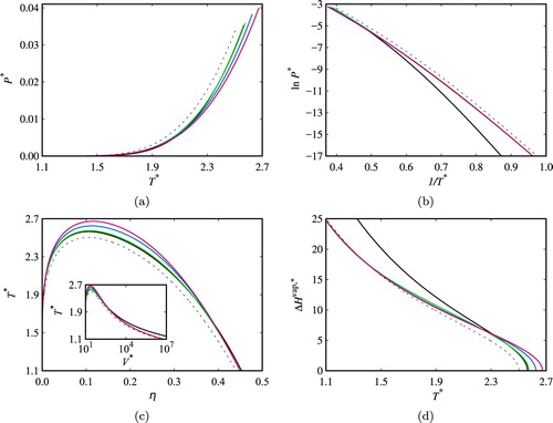
The low-temperature region of the vapour-pressure curve is better appreciated in a Clausius–Clapeyron representation (Figure 5(b)). Here, for temperatures $1/T^{\ast }>0.5$, the vapour pressures of the systems with intramolecular association are found to be close to those of the non-associating system, and are visibly larger than those of the system in which only intermolecular association is taken into account. This behaviour suggests intramolecular association is favoured at low temperatures, which results in less intermolecular association as only one bond per pair of association sites is allowed. As the formation of an intramolecular bond does not affect the number of species in the fluid, the density of the vapour and liquid phase in these conditions can be expected to be close to those of the non-associating system, leading to vapour pressures close to those of the non-associating system. This effect is confirmed by examining the temperature–density phase diagram.

The coexistence densities (in terms of packing fractions) of the liquid and vapour phases can be seen in Figure 5(c). The increase of the critical temperature of the fluids with intramolecular association is clearly seen in this figure, together with slightly wider envelopes for increasing intramolecular association in the high-temperature region of the phase diagram. At low temperature, the densities of the saturated liquid are very close for all of the associating systems (and close to those of the non-associating fluid). The impact of incorporating intramolecular association is more clearly seen by examining the saturated volume (inset Figure 5(c)), where the larger volume (smaller packing fraction) of the saturated gas phase for the system without intramolecular association can be seen, while the saturated volumes of the fluids with intramolecular association are seen to be close to that of the non-associating system.

Consistent trends are observed (Figure 5(d)) in the calculated enthalpy of vaporisation. At low temperatures ($T^{\ast }<2$), the systems with intramolecular association exhibit values of the enthalpy close to that of the non-associating system and markedly lower than those of the system with intermolecular association only. The trend is reversed in the high-temperature region partly driven by the higher critical temperature of the systems with intramolecular interactions.

In order to gain further understanding of the impact of intramolecular association on the fluid-phase behaviour of our model systems we analyse the effect of temperature and packing fraction on the distribution of aggregates. In Figure 6, we present calculations for three of the associating model fluids: associating chains in the absence of intramolecular bonding ($W^{\ast }=0$), and associating chains with intramolecular association characterised by $W^{\ast }=10$ and $W^{\ast }=100$. Low-density states are represented in Figures 6(a–c), high-density states in Figures 6(d–f), and variable density at a constant temperature of $T^{\ast }=2.0$ in Figures 6(g–i). Given the proposed association model (two sites labelled A and B, with only AB bonding allowed), molecules may be in one of three bonding states: free monomer, bonded in a linear chain aggregate, or intramolecularly bonded. In the figures, each of the fractions are represented by the width of the corresponding area. In order to appreciate better the change in the numbers of aggregate species for changing thermodynamic conditions, a broad temperature/density range is presented, including states within the two-phase envelope. On inspection it can be clearly seen that a decrease in temperature or an increase in packing fraction results in an increase of the fraction of associated molecules (given by the sum of inter- and intramolecular associated molecules), as can be expected. Moreover, regardless of the value of $W^{\ast }>0$ or packing fraction, at sufficiently low temperatures, the fractions of both monomers and molecules with intermolecular bonds are expected to approach zero and all molecules to exhibit an intramolecular bond, since such a state maximises the number of site–site interactions in the fluid. In any open-chain aggregate two sites remain unbonded, while in intramolecular hydrogen-bonded configurations, a limit with all of the sites bonded may be reached.

Figure 6. Fractions of molecules in each bonding state as a function of temperature $T^{\ast }=kT/{\epsilon }_{11}$ and packing fraction $\eta =(\pi /6)\rho m{\sigma }_{11}^3$: (a–c) in a low-density phase ($\eta =0.007$) as a function of temperature; (d–f) in a high-density phase ($\eta =0.3$) as a function of temperature; and (g–i) at fixed temperature $T^{\ast }=2.0$ as a function of packing fraction. The fraction of linear aggregates is given by the width of the solid area, the fraction of molecules with intramolecular HB by the width of the square-patterned area, and the fraction of monomers by the width of the white area. The subfigures to the left refer to the associating fluid in the absence of intramolecular HB ($W^{\ast }=0$), the subfigures in the centre to the model with $W^{\ast }=10$, and the subfigures to the right to $W^{\ast }=100$.

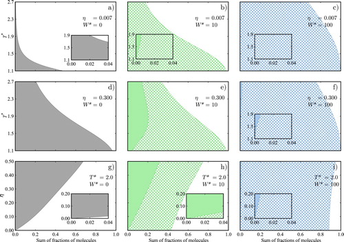
In the low-density states considered ($\eta =0.007$) few molecules are found presenting intermolecular bonds; intermolecular bonding is appreciable only at low temperatures, and principally when intramolecular association is not considered $W^{\ast }=0$ (Figures 6(a–c)). The extent of intermolecular association is dramatically reduced in the models with $W^{\ast }\ne 0$ due to the competition between inter- and intramolecular association. In the absence of intramolecular HB (Figure 6(a)), the percentage of molecules bonded is seen to reach close to 50% at the lowest temperature considered. By contrast, when intramolecular association is incorporated (Figures 6(b,c)) fewer than 0.01% of the molecules form part of open-chain aggregates, while almost all molecules present intramolecular association at the lowest temperatures. In the intermediate temperature region, a large proportion of the molecules are also found to present intramolecular HB when $W^{\ast }\ne 0$, and especially so in the case of $W^{\ast }=100$.

For the liquid-like states at $\eta =0.3$ (Figures 6(d–f)), a larger extent of association is seen throughout in comparison to the gas-like states, as a consequence of the higher density. The effect of incorporating intramolecular association is clearly appreciated when comparing the low temperature states. At $T^{\ast }=1.1$, 96% of the molecules are found to be bonded in open chains in the fluid with $W^{\ast }=0$, with only 4% for the system with $W^{\ast }=10$, and virtually no molecules forming part of open-chain aggregates for $W^{\ast }=100$, as the fluid in this case is dominated by molecules presenting intramolecular hydrogen bonds.

In the intermediate temperature region for the system with $W^{\ast }=10$, the competition of intramolecular and intermolecular association is clearly seen, with an especially interesting feature in the calculated fraction of molecules, intermolecular hydrogen bonding being the maximum that can be seen at $T^{\ast }=1.85$. At low temperatures, intramolecular bonding is favoured, even at this liquid-like density, as fewer sites remain free (unbonded) through intramolecular association than through intermolecular association, which is energetically favourable. This is particularly clear in the case of $W^{\ast }=100$ where the fluid is seen to be dominated by molecules with intramolecular bonds throughout.

Similarly, an inspection of the different bonding states as a function of packing fraction at constant temperature $T^{\ast }=2.0$ (Figure 6(g–i)) highlights the overall increase in the fraction of molecules bonded as the density increases. In terms of the ratio of molecules presenting inter- or intramolecular association, it is interesting to compare the highest packing fraction considered (${\eta }^{\ast }=0.5$), for which roughly two thirds of the molecules are found in open chains for $W^{\ast }=0$, while only 31% are in open chains for $W^{\ast }=10$, and fewer than 0.5% for $W^{\ast }=100$. As $W^{\ast }$ is increased it drives the formation of intramolecular interactions, and the fraction of molecules with intramolecular bonds increases over the entire density range.

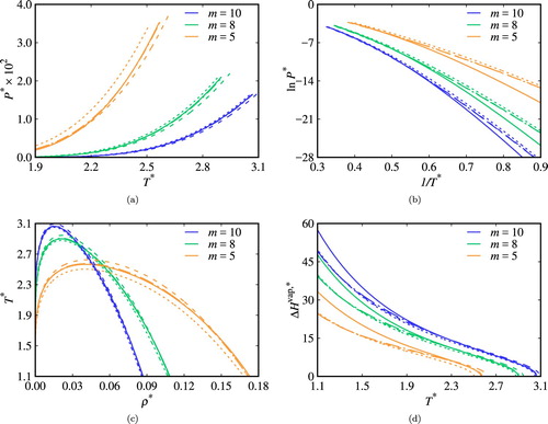
Thus far we have considered systems with a chain length of m=5. It is now interesting to consider the effect of molecular length on the phase equilibrium of the systems. Following from the models presented we have carried out fluid-phase equilibrium calculations for model chain fluids comprising m=5, m=8, and m=10 segments, considering non-associating and associating models with $W^{\ast }=0$ (no intramolecular HB), $W^{\ast }=10$, and $W^{\ast }=100$. For each chain length, the corresponding reference $W_n$ is used, so that $W^{\ast }=W/W_n$ as before, where n=m−1 is the number of links in the chain.

As can be seen in Figure 7, the expected increase in the critical temperature is observed the chain length is increased [34]. The critical temperature and pressure are seen to increase with association and more so for an increase in the likelihood of the formation of intramolecular bonds (as given by larger values of $W^{\ast }$), for all chain lengths considered. Furthermore, we note that the larger the chain length, the less impact is seen in terms of the contribution of association to the fluid-phase behaviour. This can be understood in terms of the overall free energy of the systems. For the same association energy, bonding volume and $W^{\ast }$, the contribution to the total free energy due to covalent chain formation increases with increasing m, while the value of the residual contribution from association remains comparatively unchanged. Hence, the differences in the phase behaviour between the fluids with and without ring formation are less significant for larger chains.

Figure 7. Vapour–liquid equilibria of pure chain fluids with $m=5$, $m=8$, and $m=10$ segments with interaction parameters given in Table 1: (a) vapour pressures; (b) Clausius–Clapeyron representation; (c) saturated densities; and (d) vaporisation enthalpies. The dashed curves correspond to non-associating systems, the continuous curves to systems with intermolecular association only, the long-dashed curves to those with intramolecular association with $W^{\ast }=10$, and the dash-dotted curves to those with intramolecular association with $W^{\ast }=100$.

The corresponding fractions of molecules in each of the possible bonding states are plotted in Figure 8 along the saturated liquid and vapour phase boundaries. The fraction of molecules non-bonded at any site $X_0$ markedly increases for increasing temperature and decreasing values of $W^{\ast }$ in both the liquid and vapour phases, mirroring the findings of Figure 6. The fraction of molecules associated in linear clusters is higher when intramolecular association is not considered, as can be seen in Figure 8(b), even though the fraction of non-bonded molecules is higher in these systems. In each of the systems studied, larger fractions of non-bonded molecules are seen in the gas phases, where the density is low and intramolecular association is predominant, as seen in Figure 8(b,c).

Figure 8. Temperature $T^{\ast }$ vs. (a) fraction of monomers $X_0$, (b) fraction $f_{\mathrm{chains}}$ of molecules in open-chain aggregates, and (c) fraction ${\xi }_1$ of molecules in intramolecular rings, along the saturated-vapour and liquid states for chain fluids of $m=5$, $m=8$, and $m=10$ segments. The continuous curves correspond to models with $W^{\ast }=0$, the dash-dotted curves to $W^{\ast }=10$, and the long-dashed curves to $W^{\ast }=100$.

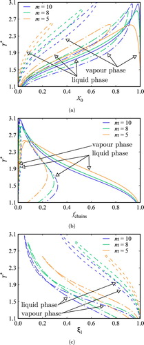
Increasing the values of $W^{\ast }$ directly promotes intramolecular bonding as seen in Figure 8(c) (and previously in Figure 6), which competes with intermolecular bonding. In Figure 8(b) the fraction of molecules involved in open chain aggregates is seen to decrease with increasing chain length. This is partly due to the molecular density of the saturated-liquid phase being lower for longer chains (Figure 7(c)), and partly due to the value of W decreasing with increasing chain length, according to Equation (97(97) $W_n=\frac{n(n-1)}{8\pi {\sigma }^3}\sum _{j=0}^k\frac{(-1{)}^j}{j!(n-j)!}{\left[\frac{n-1-2j}{2}\right]}^{n-2},$(97) ). However, this trend inverts with increasing values of $W^{\ast }$, where the fraction of molecules in open-chain aggregates is found to be smaller for the shorter chains as a result of more intramolecular association occurring for the systems with shorter chain length.

Interestingly, the saturated-vapour and liquid curves cross each other for the systems with $W^{\ast }=10$ but not for the systems with $W^{\ast }=100$ (Figure 8(c)). A higher fraction of intramolecular-bonded molecules is found in the vapour-phase for temperatures below the crossing point. At low temperatures there are more rings in the vapour than in the liquid phase because in the vapour-phase ring formation does not compete with intermolecular hydrogen bonding as in the case of the liquid phase. At $W^{\ast }=100$, the crossing of the vapour and liquid curves is no longer observed because the fraction of open-chain aggregates is insignificant in both phases.

Lastly, we consider a binary mixture of the associating chain molecules with m=5 (component 1) and a spherical component (component 2) which contains one association site of type a which can bond to a site of type b of component 1 only; no $\mathit{a}\mathit{a}$ association (dimerisation) is allowed in component 2. The parameters of the segment-segment interactions are given in Table 1. In Figure 9 we present the phase diagrams, in which vapour–liquid (VLE), liquid-liquid (LLE) equilibria, and vapour–liquid–liquid equilibria (VLLE) can be seen, together with corresponding distributions of bonding states of the chain component at a fixed pressure of $P^{\ast }=0.002$. In this model mixture, the chain component can be found in one of four bonding states: both sites non-bonded (we refer to this state as ‘free’); bonded to a spherical molecule through site B, with site A of the chain free or associated to other chains (referred to as ‘cross-associated’); bonded intermolecularly to at least one other chain molecule but not to component 2 (‘self-associated’); or intramolecularly bonded if $W^{\ast }>0$ (‘intramolecular’).

Figure 9. Fluid-phase equilibria and distribution of bonded states along the phase boundaries for a binary mixture of two-site (A and B) associating chains of m=5 segments (component 1) and spheres with one association site A (component 2), which can bond to site B in component 1 only (no AA association is allowed) at a constant pressure $P^{\ast }=0.002$. The phase boundaries are labelled as V for the saturated vapour, and L1 and L2 for the saturated liquid phases rich in component 1 and 2, respectively. The black dashed curves in (a), (b), and (c) correspond to calculations for non-associating chains, the black continuous curves to associating chains with $W^{\ast }=0$, and the coloured curves in (b) and (c) to associating chains with $W^{\ast }=10$ and $W^{\ast }=100$, respectively. The fractions of chain molecules in the possible bonding states along the saturation curves are represented in the middle and right-hand side panels. For a given temperature, the fraction of cross-associated molecules of component 1 is represented by the width of the dark-colour solid area, the fraction of self-associated molecules by the width of the light-colour solid area, the fraction of chains with intramolecular HB by the width of the square-patterned area, and the fraction of non-bonded (free) chains by the width of the white area. (a) Associating fluid in the absence of ring formation ($W^{\ast }=0$); (b) associating fluid with $W^{\ast }=10$; and (c) associating fluid with $W^{\ast }=100$.

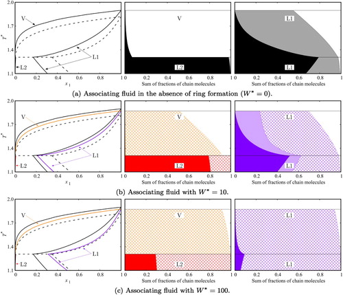
Examining the phase behaviour in Figure 9(a) it is noticeable that including cross association leads to a narrowing of the LLE region and to higher saturation temperatures of the bubble and dew curves (following the higher saturation temperature of the associating chain fluid). The overall fraction of molecules of the chain component (component 1) that are found to be bonded increases with decreasing temperature, in both the vapour and the liquid phases. Virtually no cross-association between the two components is seen in the vapour phase or in L1, in which the mole fraction of chain molecules is very small. In liquid phase L2, which is rich in chain molecules, a large fraction of cross-associated molecules is seen, which increases with the enrichment of the solution in spherical molecules.

With regards to the formation of intramolecular bonds, in the mixture with associating chains with $W^{\ast }=10$ (Figure 9(b)), a broader LLE region is seen compared to the case of the associating system with no intramolecular bonding. This is because fewer molecules of component 1 participate in cross-association with component 2 when intramolecular bonding occurs. This can be easily confirmed by studying the corresponding bonded states of the chain molecules. The overall fraction of bonded chain molecules in the L1 and L2 phase boundaries for the mixture with chains with $W^{\ast }=10$ is only slightly higher than in the previous case of the chains with no intramolecular association, but with the difference that now a large proportion of the molecules are seen to present intramolecular bonding.

The most noticeable change is seen along the vapour phase boundary. In the case of $W^{\ast }=0$ the fraction of molecules bonded is non-negligible only at lower temperatures, while in the case with $W^{\ast }=10$ between 50% (at higher temperature) and 90% (at lower temperature) of the chain molecules are seen to be intramolecularly bonded. A further feature worth highlighting refers to the L2 branch, in which the fraction of self-associated chains can be seen to remain essentially constant as the temperature is decreased, while for the case of the mixture with $W^{\ast }=0$ it can be seen to increase (Figure 9(a), right-hand panel).

Considering the mixture with chains characterised by $W^{\ast }=100$ (Figure 9(c)), similar trends as for the system with $W^{\ast }=10$ are seen, although these are of course more pronounced. The LLE boundaries and the bubble curve are found close to those of the mixture with non-associating chains, since with more intramolecular association in the system, less intermolecular and cross association occurs. The overall fraction of associated chains is found to be the largest of the three mixtures considered, in all phases, as this corresponds to the largest value of $W^{\ast }$.

7. Final remarks

The theory presented in our current work enables the modelling of chain molecules of $m\ge 1$ tangentially bonded spherical segments with embedded short-range association sites that mediate hydrogen-bond type interactions and result in the formation of closed aggregates in addition to open linear and branched aggregates. The intermolecular as well as intramolecular formation of ring-like aggregates are accounted for in the theory.

The formalism followed is that of Wertheim with the standard TPT1 steric restrictions of two sites per bond, one bond per site, and no double bonding between two segments. Wertheim's approximation neglecting closed aggregates is relaxed to allow for the contribution to the Helmholtz free energy of the formation of intramolecular bonds and intermolecular ring aggregates to be accounted for.

After imposing steric restrictions, an expression for the Helmholtz free energy of the distribution of bonding states is derived based on the aggregate count following a pedagogical approach. The mass action equations determining the distribution of bonding states at equilibrium are found by minimisation of Wertheim's expression for the Helmholtz free energy modified to include an extended fundamental graph sum to account for the closed aggregates. The theory presented is thus an extended TPT1 to treat ring-like aggregates. Two new model parameters are required per ring type: the ring size τ (i.e., number of molecules in a ring, with $\tau =1$ for an intramolecular ring) and a parameter W that captures the probability of two segments of the same molecule or of the same chain-like aggregate being within the appropriate bonding distance. As a first approximation, W is considered to be independent of density and temperature and to be specific for a pair of sites types $\mathit{a}\mathit{b}$ in a given component i (single-component rings) capable of associating to form ring-like clusters of a given size ${\tau }_R$: $W_{i,ab,{\tau }_R}$.

The free energy is presented as a residual contribution of the total Helmholtz free energy so it can be implemented in equations of state of the SAFT (and CPA) family. In particular, we have presented calculations using the SAFT-VR Mie equation of state for chains with two (AB) sites that promote both intramolecular hydrogen bonding and intermolecular association. Different chain lengths and different degrees of intramolecular association as determined by the value of W are studied and the competition between different bonding states upon the introduction of a one-site associating spherical component is also examined.

Larger values of W promote intramolecular bonding, lead to higher critical temperatures and pressures in the pure chain fluids and to higher vapour pressures at low temperatures as compared to the case of associating chains with no intramolecular bonding. Association is promoted by the decrease of temperature and at sufficiently low temperatures intramolecular bonded molecules are seen to dominate in the fluids since the number of bonds in the fluid is maximised in this configuration and hence these states are the most energetically favourable.

At intermediate temperatures the competition between inter- and intramolecular hydrogen bonding is discussed through the analysis of the distribution of bonding states. The extent of both inter- and intramolecular association decreases with the decrease of packing fraction. This effect is naturally more pronounced in terms of the intermolecular aggregates than in terms of the intramolecular association.

The extension of the association contribution presented requires the introduction of new physically-meaningful parameters since the types of rings to be considered in the system need to be specified, with a ring type characterised by its size $\tau \le 1$ ($\tau =1$ for an intramolecular bond) and its likelihood of formation W. For each ring size, the corresponding W can in principle be estimated from data derived from experiment or molecular simulation. Application of this theory to experimental systems of chemical and pharmaceutical interest will be the subject of future publications.

Sites nomenclature

$\alpha ,\delta ,\gamma ,\psi$	=	subset of association sites
$\Gamma$	=	set of association sites
$a,b,c,\dots$	=	association site types
$s,s^{\prime },s^{″},\dots$	=	individual (generic) association sites
$\mathrm{A},\mathrm{B},\mathrm{C},\dots$	=	specific (labelled) association sites
$N_{\mathrm{ST}}$	=	number of site types
$o{p}_{ab}$	=	set of ab pairs of association site (ba pairs not included)
$n_{\alpha }^a$	=	number of sites a in set α

Disclosure statement

No potential conflict of interest was reported by the authors.

ORCID

A. Aasen http://orcid.org/0000-0002-7436-5825

C. S. Adjiman http://orcid.org/0000-0002-4573-7722

G. Jackson http://orcid.org/0000-0002-8029-8868

A. Galindo http://orcid.org/0000-0002-4902-4156

Additional information

Funding

S.A.F. is grateful to the Department of Chemical Engineering of Imperial College London for the award of a PhD Scholarship. The authors acknowledge support from the Engineering and Physical Sciences Research Council (EPSRC) of the UK (Grants EP/E016340, EP/P006965 and EP/J014958) for support for the Molecular Systems Engineering group. C.S.A. is thankful to EPSRC for the award of a Leadership Fellowship (EP/J003840) and A.G. is thankful to the Royal Academy of Engineering and Lilly for support of a Research Chair (RCSRF18193). It is a great pleasure to be able to contribute to this Special Issue in honour of Peter Cummings, a wonderful friend and mentor.

Notes

1 Note that $X_{\mathrm{\varnothing }}$ does not correspond to $X_0$ because formally, $X_{\mathrm{\varnothing }}$ represents the ‘fraction of molecules with no sites free (at least)’, which includes all molecules. The quantity $X_{\mathrm{\varnothing }}$ is not seen in the expressions because the fraction of all molecules without restrictions always equals one.

2 Graph theory and lemmas for manipulations of graphs can be found in [72,73].

3 The value for the pair distribution function is typically taken at contact value since the association interactions are short ranged.

4 In Equation (53(53) $\begin{array}{rl}\frac{\mathrm{\Delta }{c}_{\mathrm{ring}}^{(0)}[\{\rho \}]}{N}& =\frac{1}{2}\sum _{a=1}^{N_{\mathrm{ST}}}\sum _{b=1}^{N_{\mathrm{ST}}}\sum _{R=1}^{N_{\mathrm{RS},\mathit{a}\mathit{b}}}\frac{1}{{\tau }_R}\\ & \times {\left[\left(\sum _{s{s}^{\prime }\in o{p}_{ab}}{X}_{s{s}^{\prime }}\right)\rho {\Delta }_{ab}\right]}^{{\tau }_R}\frac{W_{ab,R}}{\rho },\end{array}$(53) ), the summation $\left(\sum _{s{s}^{\prime }\in o{p}_{ab}}{X}_{\mathit{s}{\mathit{s}}^{\prime }}\right)$ can be written in terms of site types as $|o{p}_{ab}|X_{\mathit{a}\mathit{b}}$. We are however not carrying out this change at this stage as this expression needs to be differentiated with respect to $X_{\mathit{s}{\mathit{s}}^{\prime }}$, and not site type, in the next section.

5 As an example, take the set of all sites $\Gamma =\{{\mathrm{A}}_1,{\mathrm{A}}_2,\mathrm{B}\}$. In this model we would have $o{p}_{AB}=\{A_{1}B,A_{2}B\}$, $o{p}_{AA}=\{A_1{A}_2,A_2{A}_1\}$ and $o{p}_{BB}=\mathrm{\varnothing }$.

Appendix. Detailed expressions for selected models

Recall that the residual association contribution to the total free energy in our framework is obtained as (A1) $A^{\mathrm{assoc}}=A_{\mathrm{Wert}}-\underset{\rho \to 0}{lim}{A}_{\mathrm{Wert}}.$(A1) Here we present the equations corresponding to specific associating model systems. These specific cases allow for a system of equations that does not involve the use of the partition notation and is therefore more straight-forward to implement.

Case I – Pure fluid of chain molecules with two sites A and two sites B; i.e., $\Gamma =\{A,A,B,B\}$. The formation of intermolecular rings and intramolecular hydrogen bonding is promoted by AB association, in addition the formation of open-chain aggregates is promoted by AA, BB, and AB association. The corresponding contribution to the Helmholtz free energy due to association can be developed as follows: (A2) $\begin{array}{rl}{A}_{\mathrm{Wert}}& =NkT[\phantom{\sum _{R=1}^{N_{\mathrm{RS},\mathrm{AB}}}}\ln X_0+2-X_{\mathrm{A}}-X_{\mathrm{B}}\\ & -\sum _{R=1}^{N_{\mathrm{RS},\mathrm{AB}}}\frac{1}{{\tau }_R}{\left(4X_{\mathrm{AB}}\rho {\Delta }_{\mathrm{AB}}\right)}^{{\tau }_R}\frac{W_{\mathrm{AB},R}}{\rho }],\end{array}$(A2) (A3) $\begin{array}{rl}\underset{\rho \to 0}{lim}{A}_{\mathrm{Wert}}& =NkT[\ln X_0^{\mathrm{ideal}}+2-X_{\mathrm{A}}^{\mathrm{ideal}}-X_{\mathrm{B}}^{\mathrm{ideal}}\\ & -4X_{\mathrm{AB}}^{\mathrm{ideal}}{\Delta }_{\mathrm{AB}}^{\mathrm{ideal}}{W}_{\mathrm{AB},\mathrm{intra}}],\end{array}$(A3) (A4) $\begin{array}{rl}(X_0{)}^{-1}& ={(1+c_{\mathrm{A}})}^2{(1+c_{\mathrm{B}})}^2\\ & +4c_{\mathrm{AB}}(1+c_{\mathrm{A}})(1+c_{\mathrm{B}})+2{\left(c_{\mathrm{AB}}\right)}^2,\end{array}$(A4) (A5) $\begin{array}{rl}{X}_{\mathrm{AB}}& =X_0[(1+c_{\mathrm{A}})(1+c_{\mathrm{B}})+c_{\mathrm{AB}}],\end{array}$(A5) (A6) $\begin{array}{rl}{X}_{\mathrm{A}}& =\frac{1-2c_{\mathrm{AB}}{X}_{\mathrm{AB}}}{1+c_{\mathrm{A}}},X_{\mathrm{B}}=\frac{1-2c_{\mathrm{AB}}{X}_{\mathrm{AB}}}{1+c_{\mathrm{B}}},\end{array}$(A6) (A7) $\begin{array}{rl}(X_0^{\mathrm{ideal}}{)}^{-1}& =1+4c_{\mathrm{AB}}^{\mathrm{ideal}}+2{\left(c_{\mathrm{AB}}^{\mathrm{ideal}}\right)}^2,\end{array}$(A7) (A8) $\begin{array}{rl}{X}_{\mathrm{AB}}^{\mathrm{ideal}}& =X_0^{\mathrm{ideal}}[1+c_{\mathrm{AB}}^{\mathrm{ideal}}],\end{array}$(A8) (A9) $\begin{array}{rl}{X}_{\mathrm{A}}^{\mathrm{ideal}}& =1-2c_{\mathrm{AB}}^{\mathrm{ideal}}{X}_{\mathrm{AB}}^{\mathrm{ideal}},X_{\mathrm{B}}^{\mathrm{ideal}}=1-2c_{\mathrm{AB}}^{\mathrm{ideal}}{X}_{\mathrm{AB}}^{\mathrm{ideal}},\end{array}$(A9) (A10) $\begin{array}{rl}{c}_{\mathrm{A}}& =2\rho X_{\mathrm{A}}{\Delta }_{\mathrm{AA}}+2\rho X_{\mathrm{B}}{\Delta }_{\mathrm{AB}},\\ c_{\mathrm{B}}& =2\rho X_{\mathrm{A}}{\Delta }_{\mathrm{AB}}+2\rho X_{\mathrm{B}}{\Delta }_{\mathrm{BB}},\end{array}$(A10) (A11) $\begin{array}{rl}{c}_{\mathrm{AB}}& =\sum _{R=1}^{N_{\mathrm{RS},\mathit{a}\mathit{b}}}{\left(4X_{\mathrm{AB}}\right)}^{{\tau }_R-1}{\left(\rho {\Delta }_{\mathrm{AB}}\right)}^{{\tau }_R}\frac{W_{\mathrm{AB},R}}{\rho },\end{array}$(A11) (A12) $\begin{array}{rl}{c}_{\mathrm{AB}}^{\mathrm{ideal}}& ={\Delta }_{\mathrm{AB}}^{\mathrm{ideal}}{W}_{\mathrm{AB},\mathrm{intra}}.\end{array}$(A12) Case II – Pure fluid of chain molecules with two sites A and two sites B; i.e., $\Gamma =\{A,A,B,B\}$. The formation of intermolecular rings and intramolecular hydrogen bonding is promoted by AA association, in addition the formation of open-chain aggregates is promoted by AA, BB, and AB association. The corresponding contribution to the Helmholtz free energy due to association can be developed as follows: (A13) $\begin{array}{rl}{A}_{\mathrm{Wert}}& =NkT[\phantom{\sum _{R=1}^{N_{\mathrm{RS},\mathrm{AA}}}}\ln X_0+2-X_{\mathrm{A}}-X_{\mathrm{B}}\\ & -\frac{1}{2}\sum _{R=1}^{N_{\mathrm{RS},\mathrm{AA}}}\frac{1}{{\tau }_R}{\left(2X_{\mathrm{AA}}\rho {\Delta }_{\mathrm{AA}}\right)}^{{\tau }_R}\frac{W_{\mathrm{AA},R}}{\rho }],\end{array}$(A13) (A14) $\begin{array}{rl}\underset{\rho \to 0}{lim}{A}_{\mathrm{Wert}}& =NkT[\ln X_0^{\mathrm{ideal}}+2-X_{\mathrm{A}}^{\mathrm{ideal}}-X_{\mathrm{B}}^{\mathrm{ideal}}\\ & -X_{\mathrm{AA}}^{\mathrm{ideal}}{\Delta }_{\mathrm{AA}}^{\mathrm{ideal}}{W}_{\mathrm{AA},\mathrm{intra}}],\end{array}$(A14) (A15) $\begin{array}{rl}(X_0{)}^{-1}& ={(1+c_{\mathrm{A}})}^2{(1+c_{\mathrm{B}})}^2+c_{\mathrm{AA}}{(1+c_{\mathrm{B}})}^2,\end{array}$(A15) (A16) $\begin{array}{rl}{X}_{\mathrm{AA}}& =X_0{(1+c_{\mathrm{B}})}^2,\end{array}$(A16) (A17) $\begin{array}{rl}{X}_{\mathrm{A}}& =\frac{1-c_{\mathrm{AA}}{X}_{\mathrm{AA}}}{1+c_{\mathrm{A}}},X_{\mathrm{B}}=\frac{1}{1+c_{\mathrm{B}}},\end{array}$(A17) (A18) $\begin{array}{rl}(X_0^{\mathrm{ideal}}{)}^{-1}& =1+c_{\mathrm{AA}}^{\mathrm{ideal}},\end{array}$(A18) (A19) $\begin{array}{rl}{X}_{\mathrm{AA}}^{\mathrm{ideal}}& =X_0^{\mathrm{ideal}},\end{array}$(A19) (A20) $\begin{array}{rl}{X}_{\mathrm{A}}^{\mathrm{ideal}}& =1-c_{\mathrm{AA}}^{\mathrm{ideal}}{X}_{\mathrm{AA}}^{\mathrm{ideal}},X_{\mathrm{B}}^{\mathrm{ideal}}=1,\end{array}$(A20) (A21) $\begin{array}{rl}{c}_{\mathrm{A}}& =2\rho X_{\mathrm{A}}{\Delta }_{\mathrm{AA}}+2\rho X_{\mathrm{B}}{\Delta }_{\mathrm{AB}},\\ c_{\mathrm{B}}& =2\rho X_{\mathrm{A}}{\Delta }_{\mathrm{AB}}+2\rho X_{\mathrm{B}}{\Delta }_{\mathrm{BB}},\end{array}$(A21) (A22) $\begin{array}{rl}{c}_{\mathrm{AA}}& =\sum _{R=1}^{N_{\mathrm{RS},\mathrm{AA}}}{\left(2X_{\mathrm{AA}}\right)}^{{\tau }_R-1}{\left(\rho {\Delta }_{\mathrm{AA}}\right)}^{{\tau }_R}\frac{W_{\mathrm{AA},R}}{\rho },\end{array}$(A22) (A23) $\begin{array}{rl}{c}_{\mathrm{AA}}^{\mathrm{ideal}}& ={\Delta }_{\mathrm{AA}}^{\mathrm{ideal}}{W}_{\mathrm{AA},\mathrm{intra}}.\end{array}$(A23) Case III – Fluid mixture of N_C components. Each component i consists of chain molecules with any given set of sites ${\Gamma }_i$. The formation of intermolecular rings and intramolecular hydrogen bonding is promoted by AB association, where each ring is only allowed to involve a single component. In addition formation of open-chain aggregates is promoted by any pair-combination of sites in $\Gamma$, including AA, BB, AB, CC, AC, BC,… Here, $n_{i,\alpha }^a$ is used to represent the number of sites of type a in set α, in component i. The corresponding contribution to the Helmholtz free energy due to association can be developed as follows: (A24) $\begin{array}{rl}{A}_{\mathrm{Wert}}& =NkT\sum _{i=1}^{N_{\mathrm{C}}}{x}_i[\ln X_{i,0}+\frac{1}{2}\sum _{a=1}^{N_{\mathrm{ST},\mathit{i}}}{s}_{i,a}(1-X_{i,a})\\ & -\sum _{R=1}^{N_{\mathrm{RS},\mathrm{AB}}}\frac{1}{{\tau }_R}{\left(s_{i,\mathrm{A}}{s}_{i,\mathrm{B}}{X}_{i,\mathrm{AB}}\rho {\Delta }_{ii,\mathrm{AB}}\right)}^{{\tau }_R}\frac{W_{i,\mathrm{AB},R}}{\rho }],\end{array}$(A24) (A25) $\begin{array}{rl}\underset{\rho \to 0}{lim}{A}_{\mathrm{Wert}}& =NkT\sum _{i=1}^{N_{\mathrm{C}}}{x}_i[\ln X_{i,0}^{\mathrm{ideal}}+\frac{1}{2}\sum _{a=1}^{N_{\mathrm{ST},\mathit{i}}}{s}_{i,a}(1-X_{i,a}^{\mathrm{ideal}})\\ & -s_{i,\mathrm{A}}{s}_{i,\mathrm{B}}{X}_{\mathrm{AB}}^{\mathrm{ideal}}{\Delta }_{i,\mathrm{AB}}^{\mathrm{ideal}}{W}_{i,\mathrm{AB},\mathrm{intra}}],\end{array}$(A25) (A26) $\begin{array}{rl}(X_{i,0}{)}^{-1}& =\sum _{n=0}^{\min (s_{i,\mathrm{A}},s_{i,\mathrm{B}})}\frac{s_{i,\mathrm{A}}!s_{i,\mathrm{B}}!}{(s_{i,\mathrm{A}}-n)!(s_{i,\mathrm{B}}-n)!}{\left(c_{i,\mathrm{AB}}\right)}^n\\ & \times (1+c_{i,\mathrm{A}}{)}^{s_{i,\mathrm{A}}-n}(1+c_{i,\mathrm{B}}{)}^{s_{i,\mathrm{B}}-n}\\ & \times \prod _{\begin{array}{c}a=1\\ a\ne \{\mathrm{A},\mathrm{B}\}\end{array}}^{N_{\mathrm{ST},\mathit{i}}}{(1+c_{i,a})}^{s_{i,a}},\end{array}$(A26) (A27) $\begin{array}{rl}\frac{X_{i,\alpha }}{X_{i,0}}& =\sum _{n=0}^{\min (s_{i,\mathrm{A}}-n_{i,\alpha }^{\mathrm{A}},s_{i,\mathrm{B}}-n_{i,\alpha }^{\mathrm{B}})}\frac{(s_{i,\mathrm{A}}-n_{i,\alpha }^{\mathrm{A}})!(s_{i,\mathrm{B}}-n_{i,\alpha }^{\mathrm{B}})!}{(s_{i,\mathrm{A}}-n_{i,\alpha }^{\mathrm{A}}-n)!(s_{i,\mathrm{B}}-n_{i,\alpha }^{\mathrm{B}}-n)!}\\ & \times {\left(c_{i,\mathrm{AB}}\right)}^n(1+c_{i,\mathrm{A}}{)}^{-n}(1+c_{i,\mathrm{B}}{)}^{-n}\\ & \times \prod _{a=1}^{N_{\mathrm{ST},\mathit{i}}}{(1+c_{i,a})}^{s_{i,a}-n_{i,\alpha }^a},\alpha \subseteq {\Gamma }_i,\end{array}$(A27) (A28) $\begin{array}{rl}(X_{i,0}^{\mathrm{ideal}}{)}^{-1}& =\sum _{n=0}^{\min (s_{i,\mathrm{A}},s_{i,\mathrm{B}})}\frac{s_{i,\mathrm{A}}!s_{i,\mathrm{B}}!}{(s_{i,\mathrm{A}}-n)!(s_{i,\mathrm{B}}-n)!}{\left(c_{i,\mathrm{AB}}^{\mathrm{ideal}}\right)}^n,\end{array}$(A28) (A29) $\begin{array}{r}\frac{X_{i,\alpha }^{\mathrm{ideal}}}{X_{i,0}^{\mathrm{ideal}}}\\ & =\sum _{n=0}^{\min (s_{i,\mathrm{A}}-n_{i,\alpha }^{\mathrm{A}},s_{i,\mathrm{B}}-n_{i,\alpha }^{\mathrm{B}})}\frac{(s_{i,\mathrm{A}}-n_{i,\alpha }^{\mathrm{A}})!(s_{i,\mathrm{B}}-n_{i,\alpha }^{\mathrm{B}})!}{(s_{i,\mathrm{A}}-n_{i,\alpha }^{\mathrm{A}}-n)!(s_{i,\mathrm{B}}-n_{i,\alpha }^{\mathrm{B}}-n)!}\\ & \times {\left(c_{i,\mathrm{AB}}^{\mathrm{ideal}}\right)}^n,\alpha \subseteq {\Gamma }_i,\end{array}$(A29) (A30) $\begin{array}{rl}{c}_{i,c}& =\rho \sum _{j=1}^{N_{\mathrm{C}}}{x}_j\sum _{b=1}^{N_{\mathrm{ST},\mathit{j}}}{s}_{j,b}{X}_{j,b}{\Delta }_{ij,bc},\mathrm{for}c=\{a,A,B\}\end{array}$(A30) (A31) $\begin{array}{rl}{c}_{i,\mathrm{AB}}& =\sum _{R=1}^{N_{\mathrm{RS},\mathrm{AB}}}{\left(s_{i,\mathrm{A}}{s}_{i,\mathrm{B}}{X}_{i,\mathrm{AB}}\right)}^{{\tau }_R-1}{\left(\rho {\Delta }_{ii,\mathrm{AB}}\right)}^{{\tau }_R}\frac{W_{i,\mathrm{AB},R}}{\rho },\end{array}$(A31) (A32) $\begin{array}{rl}{c}_{i,\mathrm{AB}}^{\mathrm{ideal}}& ={\Delta }_{ii,\mathrm{AB}}^{\mathrm{ideal}}{W}_{i,\mathrm{AB},\mathrm{intra}}.\end{array}$(A32)

Case IV – Fluid mixture of N_C components. Each component i consists of chain molecules with any given set of sites ${\Gamma }_i$. Formation of intermolecular rings and intramolecular hydrogen bonding is promoted by AA association, where each ring is only allowed to involve a single component. In addition formation of open-chain aggregates is promoted by any pair-combination of $N_{\mathrm{RS},\mathrm{AA}}$, including AA, BB, AB, CC, AC, BC, … Here, $n_{i,\alpha }^a$ is used to represent the number of sites of type a in set α, in component i. The corresponding contribution to the Helmholtz free energy due to association can be developed as follows: (A33) $\begin{array}{rl}{A}_{\mathrm{Wert}}& =NkT\sum _{i=1}^{N_{\mathrm{C}}}{x}_i[\ln X_{i,0}+\frac{1}{2}\sum _{a=1}^{N_{\mathrm{ST},\mathit{i}}}{s}_{i,a}(1-X_{i,a})\\ & -\frac{1}{2}\sum _{R=1}^{N_{\mathrm{RS},\mathrm{AA}}}\frac{1}{{\tau }_R}{(s_A(s_A-1)X_{i,\mathrm{AA}}\rho {\Delta }_{ii,\mathrm{AA}})}^{{\tau }_R}\\ & \times \frac{W_{i,\mathrm{AA},R}}{\rho }\phantom{\sum _{a=1}^{N_{\mathrm{ST},\mathit{i}}}}],\end{array}$(A33) (A34) $\begin{array}{rl}\underset{\rho \to 0}{lim}{A}_{\mathrm{Wert}}& =NkT\sum _{i=1}^{N_{\mathrm{C}}}{x}_i[\ln X_{i,0}^{\mathrm{ideal}}+\frac{1}{2}\sum _{a=1}^{N_{\mathrm{ST},\mathit{i}}}{s}_{i,a}(1-X_{i,a}^{\mathrm{ideal}})\\ & -\frac{1}{2}{s}_A(s_A-1)X_{i,\mathrm{AA}}^{\mathrm{ideal}}{\Delta }_{ii,\mathrm{AA}}^{\mathrm{ideal}}{W}_{i,\mathrm{AA},\mathrm{intra}}\phantom{\sum _{i=1}^{N_{\mathrm{C}}}}],\end{array}$(A34) (A35) $\begin{array}{rl}(X_{i,0}{)}^{-1}& =\sum _{n=0}^{\lfloor \frac{s_{i,\mathrm{A}}}{2}\rfloor }\frac{s_{i,\mathrm{A}}!}{(s_{i,\mathrm{A}}-2n)!}{\left(c_{i,\mathrm{AA}}\right)}^n\\ & \times {(1+c_{i,\mathrm{A}})}^{s_{i,\mathrm{A}}-2n}\prod _{\begin{array}{c}a=1\\ a\ne \mathrm{A}\end{array}}^{N_{\mathrm{ST},\mathit{i}}}{(1+c_{i,a})}^{s_{i,a}},\end{array}$(A35) (A36) $\begin{array}{rl}\frac{X_{i,\alpha }}{X_{i,0}}& =\sum _{n=0}^{\lfloor \frac{s_{i,\mathrm{A}}-n_{i,\alpha }^{\mathrm{A}}}{2}\rfloor }\frac{(s_{i,\mathrm{A}}-n_{i,\alpha }^{\mathrm{A}})!}{(s_{i,\mathrm{A}}-n_{i,\alpha }^{\mathrm{A}}-2n)!}{\left(c_{i,\mathrm{AA}}\right)}^n{(1+c_{i,\mathrm{A}})}^{-2n}\\ & \times \prod _{a=1}^{N_{\mathrm{ST},\mathit{i}}}{(1+c_{i,a})}^{s_{i,a}-n_{i,\alpha }^a},\alpha \subseteq {\Gamma }_i,\end{array}$(A36) (A37) $\begin{array}{rl}(X_{i,0}^{\mathrm{ideal}}{)}^{-1}& =\sum _{n=0}^{\lfloor \frac{s_{i,\mathrm{A}}}{2}\rfloor }\frac{s_{i,\mathrm{A}}!}{(s_{i,\mathrm{A}}-2n)!}{\left(c_{i,\mathrm{AA}}^{\mathrm{ideal}}\right)}^n,\end{array}$(A37) (A38) $\begin{array}{rl}\frac{X_{i,\alpha }^{\mathrm{ideal}}}{X_{i,0}^{\mathrm{ideal}}}& =\sum _{n=0}^{\lfloor \frac{s_{i,\mathrm{A}}-n_{i,\alpha }^{\mathrm{A}}}{2}\rfloor }\frac{(s_{i,\mathrm{A}}-n_{i,\alpha }^{\mathrm{A}})!}{(s_{i,\mathrm{A}}-n_{i,\alpha }^{\mathrm{A}}-2n)!}{\left(c_{i,\mathrm{AA}}^{\mathrm{ideal}}\right)}^n,\alpha \subseteq {\Gamma }_i,\end{array}$(A38) (A39) $\begin{array}{rl}{c}_{i,c}& =\rho \sum _{j=1}^{N_{\mathrm{C}}}{x}_j\sum _{b=1}^{N_{\mathrm{ST},\mathit{j}}}{s}_{j,b}{X}_{j,b}{\Delta }_{ij,bc},\mathrm{for}c=\{a,A\},\end{array}$(A39) (A40) $\begin{array}{rl}{c}_{i,\mathrm{AA}}& =\sum _{R=1}^{N_{\mathrm{RS},\mathrm{AA}}}{(s_A(s_A-1)X_{i,\mathrm{AA}})}^{{\tau }_R-1}\\ & \times {\left(\rho {\Delta }_{ii,\mathrm{AA}}\right)}^{{\tau }_R}\frac{W_{i,\mathrm{AA},R}}{\rho },\end{array}$(A40) (A41) $\begin{array}{rl}{c}_{i,\mathrm{AA}}^{\mathrm{ideal}}& ={\Delta }_{ii,\mathrm{AA}}^{\mathrm{ideal}}{W}_{i,\mathrm{AA},\mathrm{intra}}.\end{array}$(A41)

References

- E. Arunan, G.R. Desiraju, R.A. Klein, J. Sadlej, S. Scheiner, I. Alkorta, D.C. Clary, R.H. Crabtree, J.J. Dannenberg, P. Hobza, H.G. Kjaergaard, A.C. Legon, B. Mennucci and D.J. Nesbitt, Pure Appl. Chem. 83 (8), 1637–1641 (2011).
- Y. Maréchal, The Hydrogen Bond and the Water Molecule (Elsevier, Amsterdam, 2007). the nether edition.
- N.G. Almarza, Phys. Rev. E 86 (3), 030101 (2012).
- P.S. Burton, R.A. Conradi, N.F.H. Ho, A.R. Hilgers and R.T. Borchardt, J. Pharm. Sci. 85 (12), 1336–1340 (1996).
- U. Domańska, Fluid Phase Equilib. 55 (1), 125–145 (1990).
- U. Domańska, Ind. Eng. Chem. Res. 29 (3), 470–475 (1990).
- C.M. Dobson, Nature 426 (6968), 884–890 (2003).
- C.N. Pace, B.A. Shirley, M. McNutt and K. Gajiwala, FASEB J. 10 (1), 75–83 (1996).
- R.E. Hubbard and M.K. Haider, Hydrogen Bonds in Proteins: Role and Strength, 2010.
- A.N. Semenov, A.N. Semenov, I.A. Nyrkova and M.E. Cates, Macromolecules 28 (23), 7879–7885 (1995); I.A. Nyrkova, and M.E. Cates. Macromolecules, 28 (23), 7879–7885 (1995).
- M. Rubinstein and A.V. Dobrynin, Curr. Opin. Colloid Interface Sci. 4 (1), 83–87 (1999).
- P.J.M. Stals, M.A.J. Gillissen, R. Nicolaÿ, A.R.A. Palmans and E.W. Meijer, Polym. Chem. 4 (8), 2584–2597 (2013).
- C.J. Gregg, F.P. Stein and M. Radosz, Macromolecules 27 (18), 4972–4980 (1994).
- C.J. Gregg, F.P. Stein and M. Radosz, Macromolecules 27 (18), 4981–4985 (1994).
- F. Dolezalek, Zeitschrift für Phys. Chemie 64 (1), 727 (1908).
- H.C. Andersen, J. Chem. Phys. 59 (9), 4714–4725 (1973).
- H.C. Andersen, J. Chem. Phys. 61 (12), 4985–4992 (1974).
- D. Chandler and L.R. Pratt, J. Chem. Phys. 65 (8), 2925–2940 (1976).
- J.S. Høye and K. Olaussen, Phys. A Stat. Mech. Appl. 104 (3), 435–446 (1980).
- P.T. Cummings and G. Stell, Mol. Phys. 51 (2), 253–287 (1984).
- P.T. Cummings and G. Stell, Mol. Phys. 55 (1), 33–48 (1985).
- P.T. Cummings and G. Stell, Mol. Phys. 60 (6), 1315–1342 (1987).
- S.H. Lee, P.T. Cummings and G. Stell, Mol. Phys. 62 (1), 65–90 (1987).
- H.C. Andersen and D. Chandler, J. Chem. Phys. 57 (5), 1918–1929 (1972).
- D. Chandler and H.C. Andersen, J. Chem. Phys. 57 (5), 1930–1937 (1972).
- M.S. Wertheim, J. Stat. Phys. 35 (1–2), 19–34 (1984).
- M.S. Wertheim, J. Stat. Phys. 35 (1–2), 35–47 (1984).
- M.S. Wertheim, J. Stat. Phys. 42 (3–4), 459–476 (1986).
- M.S. Wertheim, J. Stat. Phys. 42 (3–4), 477–492 (1986).
- W.G. Chapman, K.E. Gubbins, C.G. Joslin and C.G. Gray, Fluid Phase Equilib. 29, 337–346 (1986).
- C.G. Joslin, C.G. Gray, W.G. Chapman and K.E. Gubbins, Mol. Phys. 62 (4), 843–860 (1987).
- W.G. Chapman, K.E. Gubbins, C.G. Joslin and C.G. Gray, Pure Appl. Chem. 59 (1), 53–60 (1987).
- G. Jackson, W.G. Chapman and K.E. Gubbins, Mol. Phys. 65 (1), 1–31 (1988).
- W.G. Chapman, G. Jackson and K.E. Gubbins, Mol. Phys. 65 (5), 1057–1079 (1988).
- F. Sciortino, E. Bianchi, J.F. Douglas and P. Tartaglia, J. Chem. Phys. 126 (19), 194903 (2007).
- J. Russo, P. Tartaglia and F. Sciortino, Soft. Matter. 6 (17), 4229 (2010).
- J.M. Tavares, P.I.C. Teixeira, M.M. Telo da Gama and F. Sciortino, J. Chem. Phys. 132 (23), 234502 (2010).
- H. Liu, S.K. Kumar, F. Sciortino and G.T. Evans, J. Chem. Phys. 130 (4), 044902 (2009).
- S. Roldán-Vargas, F. Smallenburg, W. Kob and F. Sciortino, J. Chem. Phys. 139 (24), 244910 (2013).
- M.S. Wertheim, J. Chem. Phys. 87 (12), 7323–7331 (1987).
- R. Dickman and C.K. Hall, J. Chem. Phys. 89 (1), 3168 (1988).
- W.G. Chapman, K.E. Gubbins, G. Jackson and M. Radosz, Fluid Phase Equilib. 52, 31–38 (1989).
- W.G. Chapman, K.E. Gubbins, G. Jackson and M. Radosz, Ind. Eng. Chem. Res. 29 (8), 1709–1721 (1990).
- I.G. Economou and M.D. Donohue, AIChE J. 37 (12), 1875–1894 (1991).
- Y.S. Wei and R.J. Sadus, AIChE J. 46 (1), 169–196 (2000).
- E.A. Müller and K.E. Gubbins, Ind. Eng. Chem. Res. 40 (10), 2193–2211 (2001).
- I.G. Economou, Ind. Eng. Chem. Res. 41 (5), 953–962 (2002).
- S.P. Tan, H. Adidharma and M. Radosz, Ind. Eng. Chem. Res. 47 (21), 8063–8082 (2008).
- G.M. Kontogeorgis and G.K. Folas, In Thermodyn. Model. Ind. Appl., (John Wiley & Sons, Ltd, 2009), pp. 221–259.
- C. McCabe and A. Galindo, In Appl. Thermodyn. Fluids, edited by A.R.H Goodwin and J.V Sengers (The Royal Society of Chemistry, 2010), Chap. 8, pp. 215–279.
- K.E. Gubbins, Mol. Phys. 111 (24), 3666–3697 (2013).
- R.P. Sear and G. Jackson, Phys. Rev. E 50 (1), 386–394 (1994).
- R.P. Sear and G. Jackson, Mol. Phys. 87 (2), 517–521 (1996).
- D. Ghonasgi, V. Perez and W.G. Chapman, J. Chem. Phys. 101 (8), 6880–6887 (1994).
- D. Ghonasgi and W.G. Chapman, J. Chem. Phys. 102 (6), 2585–2592 (1995).
- A.J. García-Cuéllar and W.G. Chapman, Mol. Phys. 96 (7), 1063–1074 (1999).
- A.S. Avlund, PhD thesis, Technical University of Denmark, 2011.
- A.S. Avlund, G.M. Kontogeorgis and W.G. Chapman, Mol. Phys. 109 (14), 1759–1769 (2011).
- A. Galindo, S.J. Burton, G. Jackson, D.P. Visco and D.A. Kofke, Mol. Phys. 100 (14), 2241–2259 (2002).
- A.J. García-Cuéllar, D. Ghonasgi and W.G. Chapman, Fluid Phase Equilib. 116 (1–2), 275–281 (1996).
- A.S. Avlund, G.M. Kontogeorgis and M.L. Michelsen, Ind. Eng. Chem. Res. 51 (1), 547–555 (2012).
- B.D. Marshall, A.J. García-Cuéllar and W.G. Chapman, J. Chem. Phys. 136 (15), 154103 (2012).
- B.D. Marshall, A.J. García-Cuéllar and W.G. Chapman, J. Chem. Phys. 138 (20), 204908 (2013).
- D. Ballal and W.G. Chapman, J. Phys. Chem. B 119 (22), 6792–6802 (2015).
- J.M. Tavares, L. Rovigatti and F. Sciortino, J. Chem. Phys. 137 (4), 44901 (2012).
- L. Rovigatti, J.M. Tavares and F. Sciortino, Phys. Rev. Lett. 111 (16), 168302 (2013).
- J.M. Tavares, N.G. Almarza and M.M. Telo da Gama, J. Chem. Phys. 140 (4), 044905 (2014).
- J.M. Tavares, N.G. Almarza and M.M. Telo da Gama, Soft. Matter. 11 (29), 5828–5838 (2015).
- T. Lafitte, A. Apostolakou, C. Avendaño, A. Galindo, C.S. Adjiman, E.A. Müller and G. Jackson, J. Chem. Phys. 139 (15), 154504 (2013).
- C.G. Gray and K.E. Gubbins, Theory of Molecular Fluids, Vol:1, Fundamentals (Oxford University Press, Oxford 1984).
- T.L. Hill, J. Chem. Phys. 23 (4), 617–622 (1955).
- J.P. Hansen and I.R. McDonald, Theory of Simple Liquids 4th Edition (Academic Press, Oxford 2013).
- W. Zmpitas and J. Gross, Fluid Phase Equilib. 428, 121–152 (2016).
- R.P. Sear and G. Jackson, Mol. Phys. 81 (4), 801–811 (1994).
- B.D. Marshall and W.G. Chapman, J. Phys. Chem. B 115 (50), 15036–15047 (2011).
- S.A. Febra, PhD thesis, Imperial College London, 2018.
- L.R.G. Treloar, Trans. Faraday Soc. 42, 77–82 (1946).
- P.J. Flory, Statistical Mechanics of Chain Molecules (Interscience Publishers, New York 1969).
- S. Dufal, T. Lafitte, A.J. Haslam, A. Galindo, G.N.I. Clark, C. Vega and G. Jackson, Mol. Phys. 113 (9–10), 948–984 (2015).
- S. Dufal, T. Lafitte, A.J. Haslam, A. Galindo, G.N.I. Clark, C. Vega and G. Jackson, Mol. Phys. 116 (2), 283–285 (2018).
- S. Dufal, V. Papaioannou, M. Sadeqzadeh, T. Pogiatzis, A. Chremos, C.S. Adjiman, G. Jackson and A. Galindo, J. Chem. Eng. Data 59 (10), 3272–3288 (2014).