Machine learning for collective variable discovery and enhanced sampling in biomolecular simulation

Abstract

Classical molecular dynamics simulates the time evolution of molecular systems through the phase space spanned by the positions and velocities of the constituent atoms. Molecular-level thermodynamic, kinetic, and structural data extracted from the resulting trajectories provide valuable information for the understanding, engineering, and design of biological and molecular materials. The cost of simulating many-body atomic systems makes simulations of large molecules prohibitively expensive, and the high-dimensionality of the resulting trajectories presents a challenge for analysis. Driven by advances in algorithms, hardware, and data availability, there has been a flare of interest in recent years in the applications of machine learning – especially deep learning – to molecular simulation. These techniques have demonstrated great power and flexibility in both extracting mechanistic understanding of the important nonlinear collective variables governing the dynamics of a molecular system, and in furnishing good low-dimensional system representations with which to perform enhanced sampling or develop long-timescale dynamical models. It is the purpose of this article to introduce the key machine learning approaches, describe how they are married with statistical mechanical theory into domain-specific tools, and detail applications of these approaches in understanding and accelerating biomolecular simulation.

GRAPHICAL ABSTRACT

Keywords:

• machine learning
• molecular simulation
• deep learning
• enhanced sampling
• collective variables

1. Introduction

Classical molecular dynamics (MD) simulation is a workhorse tool for the study of molecular and atomic systems to understand and predict their behaviour by integrating Newton's equations of motion at the molecular scale [1,2]. The essence of the technique is to simulate the dynamical evolution of a molecular system through its phase space spanned by the atomic positions and velocities under a Hamiltonian defining the many-body interaction potential. Analysis of the resulting simulation trajectories provides a means to estimate the structural, thermodynamic, and dynamical properties of the system. Performing a molecular dynamics requires three chief ingredients: an initial system configuration, an interaction potential, and a means to integrate the classical equations of motion. This approach was anticipated in 1812 by Pierre Simon de Laplace's Gedankenexperiment that posited ‘an intelligence which could comprehend all the forces by which nature is animated and the respective positions of the beings which compose it, if moreover this intelligence were vast enough to submit these data to analysis … to it nothing would be uncertain, and the future as the past would be present to its eyes’ [3]. Alder and Wainwright were the first to realise Laplace's ‘clockwork universe’ in 1957 through their pioneering molecular dynamics simulations employing state-of-the-art computers and simulation algorithms to approximate the role of the ‘all-seeing intelligence’ [4,5]. Modern advances in computational hardware and software and force fields constructed from quantum mechanical calculations and precise experimental measurements have enabled simulations of systems of billions [6,7] and even trillions [8] of atoms. However, validated force fields for arbitrary materials and conditions are still lacking, and the inherently serial nature of numerical integration and the requirement for short time steps on the order of femtoseconds to preserve numerical stability have largely limited simulations of non-trivial systems to millisecond time scales [9–11]. Karplus and Petsko elegantly articulated these deficiencies in their 1990 article with their assertion holding equally true today [12]: ‘Two limitations in existing simulations are the approximations in the potential energy functions and the lengths of the simulations. The first introduces systematic errors and the second statistical errors.’ The continued success of MD is critically contingent on progress on both of these fronts and each is an important and active area of research in the field. The present review considers recent advances enabled by machine learning in general, and deep learning in particular, in engaging the second of these challenges.

The statistical errors in structural, thermodynamic, and kinetic properties is fundamentally a sampling problem. Simulation trajectories furnished by standard MD do not offer sufficiently comprehensive sampling of the states or events of interest to provide robust estimations of the properties of interest [11,12]. Proper sampling of the relevant states and transition rates is critical for the success of biomolecular simulations in applications including identification of the native and metastable states of a protein, resolution of protein binding pockets and association free energy of ligands and drugs, prediction of the permeability of membrane modulating peptides, understanding of the mechanisms of protein allostery, prediction of the stable structures and aggregation pathways of self-assembling peptides, and modelling of the activation pathways and kinetics of membrane proteins. Enhanced sampling techniques presently engage this challenge with approaches that fall largely into one of four classes [13–20]. (I) Path sampling techniques that efficiently sample reactive pathways between two pre-defined states. (II) Tempering or generalised ensemble approaches that modify the system Hamiltonian to lower barrier heights and improve sampling of configurational space. (III) Decomposition techniques that break the (configurational) phase space of the system into a number of disjoint metastable states and construct a kinetic model for the dynamical transitions between these states. (IV) Collective variable (CV) biasing techniques that accelerate sampling and barrier hopping along pre-specified order parameters.

The first class of approaches – path sampling – focuses on sampling the interconversion pathways between two defined states of interest, making it less well suited to the global exploration of a previously uncharted configurational space. Recent work by Bolhuis and co-workers combining path reweighting with transition path sampling has, however, demonstrated a means to estimate the underlying free energy surface in the vicinity of the barrier and terminal states [21].

The second class of approaches – tempering – is well suited to systems for which there is very little prior knowledge as to what collective variables are most important in governing the system dynamics, but suffer from the drawback that much computational effort is expended sampling modified Hamiltonians that are generally not of direct interest but serve only to support improved sampling [13].

The third class of approaches – discrete kinetic models – requires the definition of a partitioning of phase space into a set of disjoint metastable states and therefore requires sampling of these thermally-relevant configurations. As such, methods from the second or fourth classes of techniques are profitably employed to efficiently sample the configurational space rather than relying upon the exploration provided by unbiased simulations.

The fourth class of approaches – collective variable biasing – appears to suffer from the deficiency that they presuppose the availability of ‘good’ CVs along which to drive sampling. We define ‘good’ in the sense that driving sampling along these CVs leads to lower variance estimators of the structural, thermodynamic, or kinetic properties of interest [23–26]. As such, these CVs should typically be coincident with or closely related to the important dynamical motions of the system and drive sampling over free energy barriers connecting thermally relevant states that would be rarely be surmounted in unbiased simulations. For all but the simplest systems it is not possible to intuit good CVs [27,28], and accelerating bad CVs that are irrelevant to the important molecular motions can lead to poorer sampling than standard unbiased MD. For this reason, the development of techniques to determine good CVs for enhanced sampling is of ‘paramount concern in the continued evolution of such methods’ [13]. In 2018 we published a review of nonlinear machine learning approaches for data-driven CV discovery [16]. It is the purpose of the present review to provide an update to this fast moving field and illuminate some recent advances in employing tools from machine learning – deep learning in particular – for CV discovery and enhanced sampling. We also direct the interested reader to a number of other recent reviews of machine learning in molecular simulation [29], soft materials engineering [30,31], materials science [32], collective variable identification [33], and enhanced sampling [13].

The structure of this review is as follows. In Section 2, we present a brief survey of some of the most prevalent and powerful machine learning techniques that have found broad adoption within the molecular simulation community. Building upon these fundamentals, in Section 3 we detail recent advances in CV discovery and enhanced sampling enabled by these machine learning tools. We focus our discussion upon biomolecular simulations, and in particular protein folding, where many of these developments and successes have been demonstrated. We will largely focus on all-atom simulations where the sampling problem is most severe, but all techniques discussed may be equally well applied to coarse-grained calculations. Finally, in Section 4 we present our outlook upon emerging challenges and opportunities for the field.

2. Survey of popular machine learning techniques for CV discovery

The data-driven CVs sought for enhanced sampling are those which provide improved statistical estimates of the properties of interest. Typically, these CVs are correlated with the highest-variance or slowest-evolving collective degrees of freedom, and therefore can also provide molecular-level insight and understanding of system properties and behaviour. In principle, enhanced sampling could be conducted in all possible combinations of CVs and those which provide the statistically optimal estimates of the property we seek to estimate declared the ‘best’. Of course the enormous computational cost associated with a blind search in the combinatorial space of all possible CVs entirely defeats the purpose of enhanced sampling to provide efficient and accelerated property estimation. Accordingly, a constructive criterion by which to define and determine a ‘good’ CV is required [34–36]. Putative CVs can be considered order parameters spanning a reduced-dimensional subspace of the molecular configurational space. The quality of the subspace defined by these CVs is frequently scored according to one of two common metrics: high-variance CVs parameterise a subspace that maximally preserves the configurational variance contained within a molecular simulation trajectory [37–39], whereas slow CVs (i.e. highly autocorrelated CVs) span a subspace that maximally preserves the kinetic content.

High-variance CV discovery is more straightforward and amenable to a wide array of established machine learning and dimensionality reduction techniques. Data-driven discovery of these CVs take simulation trajectories as their input, and it is typically possible to apply these techniques to non-time ordered data and data generated by biased sampling where the thermodynamic bias can be exactly cancelled by thermodynamic reweighting [40]. Conceptually, these techniques can be thought of as identifying and parameterising a low-dimensional subspace within the high-dimensional configurational phase space to which the simulation data are approximately restrained [41,42]. We note here the apparent ‘chicken and egg’ problem wherein CV discovery requires simulation trajectories that provide good sampling of the thermally relevant phase space, whereas the generation of such trajectories requires enhanced sampling in good CVs [33]. The solution, of course, is to iterate between rounds of CV discovery and enhanced sampling until convergence of the CVs and phase space exploration [33,37,43,44].

The application of machine learning for high-variance CV discovery was pioneered through the use of linear dimensionality reduction tools such as principal component analysis (PCA) and multidimensional scaling (MDS) [45,46]. However, the inherent linearity of these approaches limited the capabilities in identifying the important nonlinear CVs characteristic of complex molecular systems. In more recent years, nonlinear dimensionality reduction and manifold learning techniques have been employed, including locally linear embedding (LLE) [47,48], Isomap [49–52], local tangent space alignment [53], Hessian eigenmaps [54], Laplacian eigenmaps [55], diffusion maps (DMAPS) [41, 44,56–58], sketch maps [38,59,60] and t-distributed Stochastic Neighbor Embedding (t-SNE) [61]. These more powerful techniques have largely superseded linear approaches but do tend to suffer from the absence of an explicit functional mapping of atomic coordinates to the CVs, which can present challenges in interpretability and implementing biased sampling [37,43,44,62, 63]. Deep learning techniques based on artificial neural networks have recently emerged as a means to discover high-variance nonlinear CVs that are equipped with explicit and differentiable functional mappings to the atomic coordinates [37,64].

Slow CV discovery tends to be more challenging and approachable with a narrower class of machine learning tools. These approaches are also more restrictive in that they typically require (long) time-ordered trajectories that have been propagated under the unbiased system Hamiltonian. Depending on the particular dynamical propagator that is implemented, approaches do exist to relax the requirement for unbiased trajectories by performing dynamical reweighting of biased simulation trajectories [65–70]. Conceptually, these approaches seek linear or nonlinear functions of the configurational coordinates that are maximally autocorrelated and therefore parameterise the slowest-evolving molecular motions. In general, these approaches owe their mathematical foundations to the properties of the transfer operator (a.k.a. Perron-Frobenius operator or propagator) or its adjoint the Koopman operator [71–83] and associated variational principles such as the variational approach to conformational dynamics (VAC) [84,85] or variational approach to Markov processes (VAMP) [80]. Classical techniques for slow CV discovery include time-lagged independent component analysis (TICA) [86,87] kernel TICA (kTICA) [88,89], dynamical mode decomposition (DMD) [74,90–96], extended dynamical mode decomposition (EDMD) [78,97,98], canonical correlation analysis (CCA) [80,99], Markov state models (MSMs) [19,20], or Ulam's method [71,100–103]. More recent approaches based on deep learning include deep CCA [104], variational approach to Markov processes networks (VAMPnets) [81,105], state-free reversible VAMPnets (SRVs) [106,107], time-lagged autoencoders (TAEs) [108,109], and variational dynamics encoders (VDEs) [109–111].

In the remainder of this section we survey four of the most popular machine learning techniques – ANNs, DMAPS, MSMs, and TICA – that serve as the foundations for many recent methodological developments in high-variance and slow CV discovery and enhanced sampling that we discuss in Section 3.

2.1. Artificial neural networks (ANNs)

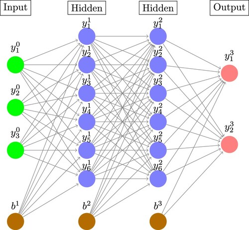
Artificial neural networks (ANNs) are collections of activation functions, or neurons, which are composited together into layers in order to approximate a given function of interest [112]. Their utility and power can be largely attributed to the universal approximation theorem, [113,114], which states that, under mild assumptions, there exists a finite-size neural network that is capable of approximating any continuous function to arbitrary precision. In a fully-connected ANN, the neurons in each layer take as their inputs the outputs from the previous layer, apply a nonlinear activation function, and pass on their outputs to the next layer. A schematic diagram of a three-layer feed-forward fully-connected neural network in Figure 1. Mathematically, the output $y_i^k$ from neuron i of fully connected layer k is given by, (1) $y_i^k=f(\sum _{j=1}^N{w}_{ji}^k{y}_j^{k-1}+b_i^k),$(1) where $w_{ji}^k$ and $b_i$ define the layer weights and biases, respectively. The activation function $f(x)$ is an arbitrary nonlinear function but is often taken to be $\tanh (x)$ or some form of rectified linear unit (ReLU) and is applied element-wise to the input. ANNs are typically trained by minimising an objective function (also called loss function) using some variant of stochastic gradient descent through a process known as backpropagation [115–117].

Figure 1. Schematic diagram of a three-layer fully-connected feed-forward neural network. The output of neuron i from layer k is denoted $y_i^k$ and the bias node for layer k denoted $b^k$. The arrows connecting pairs of neurons are the trainable weights $w_{ji}$. The output of each layer is computed from a weighted sum of outputs of the previous layer passed through a nonlinear activation function (Equation (1(1) $y_i^k=f(\sum _{j=1}^N{w}_{ji}^k{y}_j^{k-1}+b_i^k),$(1) )). (Image constructed using code downloaded from http://www.texample.net/tikz/examples/neural-network with the permission of the author Kjell Magne Fauske.)

Many of the advances in deep learning have been driven by novel network topologies, activation functions, and loss functions adapted to particular tasks. For example, convolutional neural networks capture spatial invariance of local features, a useful feature for image analysis [118–120]. Autoassociative neural networks perform non-linear dimensionality reduction [121]. Generative models, such as variational autoencoders [122] and generative adversarial networks (GANs) [123], are capable of synthesising new, unobserved examples that resemble existing training data. In applications to molecular systems, ANNs have been used to build biasing potentials for enhanced sampling [124–128], fit ab initio potential energy surfaces [129,130] and determine quantum mechanical forces in MD simulations [131], perform coarse graining [132], and generate realistic molecular configurations [133–135]. To highlight a few specific examples, PotentialNet is a novel neural network architecture which uses graph convolutions to encode molecular structures, accommodating permutation invariance and molecular symmetries [136]. SchNet is a variant of a deep tensor neural network that eliminates rotational, translational, and permutational atomic symmetries by construction and has been used to fit molecular potential energy landscapes and molecular force fields [137]. PointNet [138] is a network designed to ingest and process point cloud data for object classification and part segmentation that eliminates permutational invariances by max pooling, and which recently found applications in local molecular structure analysis and crystal structure classification [139]. CGnets learn free energy functions and force fields for coarse-grained molecular representations by fitting against all-atom force data [132]. Boltzmann Generators (BG) employ a synthesis of deep learning, normalising flows, and statistical mechanics to train an invertible network capable of efficiently sampling molecular configurations from the equilibrium distribution [133]. As we will see below, many cutting-edge ML approaches rely upon some form of ANN, and, with increasing frequency, deep neural networks (DNN) comprising many hidden layers.

We note that Boltzmann Generators [133] represent a particularly promising and powerful enhanced sampling technique for molecular systems, and although they do not inherently rely upon the discovery or definition of CVs for their operation we identify strong synergies between these techniques. First, training of BGs generally requires a number of examples of molecular structures from metastable states of the system and CV enhanced sampling techniques may be used to efficiently furnish these training examples starting from nothing more than a single structure and a molecular force field. Second, since BGs can efficiently sample and estimate free energy differences between distantly separated states of the molecular system they may be used to efficiently generate physically realistic transition pathways between metastable states identified by CV enhanced sampling. Third, one mode of BG deployment augments the network loss function with a “reaction-coordinate loss” to promote sampling along a particular direction in phase space. CV discovery techniques can identify good reaction coordinates linking important metastable states of the system. Fourth, CV discovery and enhanced sampling may be conducted within the BG latent space to augment the power of BGs to explore previously unsampled regions of configurational space through the invertible transformation to molecular coordinates.

2.2. Diffusion maps (DMAPS)

Diffusion maps are a dimensionality reduction technique originally proposed by Coifman and Lafon that performs nonlinear dimensionality reduction by harmonic analysis of a discrete diffusion process (random walk) constructed over a high-dimensional dataset [57,140]. The first application of DMAPS to molecular simulations demonstrated its capacity to extract dynamically-relevant collective molecular motions [41], and it has since seen widespread adoption as a method for the analysis of molecular trajectories [28,58,141] and as a component of adaptive biasing methods [43,44,56,63]. Mathematically, DMAPS construct a random walk over the space of molecular configurations recorded over the course of a molecular simulation, which, in the continuum limit, can be shown to correspond to a Fokker-Plank (FP) diffusion process in the presence of potential wells [142]. The leading eigenvectors of the Markov matrix describing the dynamics of the discrete random walk approximate the leading eigenfunctions of the associated backward FP operator describing the most slowly relaxing modes of the diffusion process [140]. The algorithm proceeds by constructing a kernel matrix K defined as, (2) $K_{ij}=\exp (-\frac{d(i,j{)}^2}{2ϵ}).$(2) where i and j index over molecular configurations, $d(i,j)$ is a user-defined distance metric such as the translationally and rotationally aligned root mean squared deviation (RMSD) between atomic coordinates, and ε is the user-defined kernel bandwidth which represents the characteristic step size of the random walk over the data [42]. After row-normalising the kernel matrix to conserve hopping probabilities, a spectral decomposition gives eigenvector/eigenvalue pairs that are truncated at a gap in the eigenvalue spectrum. The resultant top k eigenvectors define the CVs spanning the low-dimensional embedding and which parameterise the intrinsic manifold upon which the diffusion process is effectively restrained. The naïve implementation of DMAPS scales quadratically in the number of data points, and so variants with reducted memory and computational costs have been developed, including landmark diffusion maps (L-DMAPS) [143] and pivot diffusion maps (P-DMAPS) [144].

Although a powerful nonlinear dimensionality reduction technique, DMAPS possess at least two limitations in its applications to molecular systems. The first is the assumption of diffusive dynamics over the high-dimensional data, which may or may not be a good approximation of the true molecular dynamics. The second is the absence of an explicit mapping from the atomic coordinates to the low-dimensional CVs. As a result, out of sample extension to new data points outside of the training set require the use of approximate interpolation techniques such as the Nyström extension, Laplacian pyramids, or kriging [145–147]. Further, although the existence of an explicit function mapping is no guarantee of interpretability (consider ANNs), its absence can frustrate interpretability of the CVs. A degree of interpretability can be recovered by correlating the DMAPS CVs with candidate physical variables [41,56], perhaps within an automated search procedure [27, 148, 149], by projecting representative molecular configurations over the low-dimensional embedding, or by visualising the collective modes in the high-dimensional space [150, 151]. The absence of an explicit mapping also precludes the calculation of exact derivates of this expression, which renders diffusion maps incompatible with enhanced sampling methods such as umbrella sampling [152] or metadynamics [23] that require the gradients of the collective variables with respect to the atomic coordinates.

2.3. Markov state models (MSMs)

Markov state models (MSMs) are a powerful framework to gain insight from molecular simulation trajectories, and guide efficient simulations [20,153]. MSMs are widely used for studying many biomolecular processes including protein folding, protein association, ligand binding, and forging connections with experiment [154, 155]. Constructing MSMs typically follows the following steps: feature extraction from the molecular simulation trajectory, feature transformation, engineering, and elimination of symmetries (e.g. translation, rotation, permutation), projection of engineered features into a low-dimensional subspace, clustering low-dimensional projections of configurations into microstates, construction of a microstate transition matrix, coarse-graining into macrostates, validation and analysis of the microstate and macrostate kinetic models for thermodynamic and dynamic properties. A schematic illustration of this pipeline is presented in Figure 2.

Figure 2. Schematic diagram of the Markov state model (MSM) construction and analysis pipeline. (a) Many short molecular dynamics trajectories are collected. (b) The snapshots constituting each trajectory are featurized, projected into a low-dimensional space, and clustered into microstates. Each frame in each trajectory is assigned to a microstate. For illustrative purposes, four microstates are considered and coloured green, blue, purple, and pink. (c) Counting the number of transitions between microstates furnishes the transition counts matrix. (d) Assuming the system is at equilibrium and therefore follows detailed balance, the count matrix is symmetrised and normalised to generate the reversible transition matrix defining the conditional transition probabilities between microstates. (e) The equilibrium distribution over microstates is furnished by the leading eigenvector of the transition probability matrix, here illustrated in a pie chart. States with greater populations are more thermodynamically stable. (f) The higher eigenvectors correspond to a hierarchy of increasingly fast dynamical relaxations over the microstates. The first of these possess a negative entry corresponding to the green state and positive entries for the other states, therefore characterising the net transport of probability distribution out of the green microstate and into the blue, purple, and pink. If desired, the microstates can be further coarse grained into macrostates, typically by clustering of the microstate transition matrix. Image reprinted with permission from Ref. [20]. Copyright (2018) American Chemical Society.

There are many important aspects in each of these steps, a detailed discussion of which can be found in Refs. [20,153,156]. Here we observe a few key points. The chief advantage of MSMs in furnishing long-time kinetic models, is that the simulation data required for their construction need only have reached local equilibrium, in the sense that the transition probabilities between neighbouring microstates are memoryless, allowing the MSM to be constructed exclusively from conditional probabilities that the system appears in state j at time $(t+\tau )$ given that system appears in state i at time t [155–158]. This is an extremely valuable property since it alleviates the need for globally equilibrated simulation trajectories that can be exceedingly expensive to generate. As such, MSMs can be constructed from multiple relatively short trajectories that can be performed in parallel and initialised adaptively to provide good sampling of all relevant transitions [156,158]. We also observe that many steps in the MSM construction pipeline profitably employ other machine learning methods. In particular, TICA, SRVs, and VDEs are frequently used in the featurization and dimensionality reduction steps [87,107,110] (see Sections 2.4 and 3.7), spectral clustering is employed to lump microstates into macrostates [159], maximum likelihood estimation used to enforce reversibility [156], and active learning used to adaptively direct sampling of undersampled microstate transitions [153]. VAMPnets and Deep Generative Markov State Models are two recently-proposed approaches that employ deep learning to replace some or all of the MSM parameterisation pipeline for the construction of discrete kinetic models. We discuss these approaches in Section 3.8.

2.4. Time-lagged independent component analysis (TICA)

Time-lagged independent component analysis (TICA) (also known as second order ICA or time-structure based ICA, and equivalent to CCA employing time-lagged data for reversible processes [104,105,108]) is a linear dimensionality reduction method that takes as input a featurization of a molecular simulation trajectory and identifies maximally autocorrelated linear projections along which the dynamical evolution of the system relaxes most slowly [71,84–87,160–164]. This stands in contrast to PCA, which identifies linear projections along which the configurational variance in the simulation trajectory is maximal [45,46,165]. The leading TICA components can be interpreted, within the linear approximation, as the leading ‘slow modes’ whereas the PCA components are the leading ‘high variance modes’. It can be shown that given a (possibly nonlinear) mean-zeroed featurization $\mathit{\xi }(\mathbf{x})=\{{\xi }_k(\mathbf{x})\}$ of the snapshots of a molecular simulation trajectory $\mathbf{x}$ with frames recorded at a time interval τ, the expansion coefficients $\mathbf{u}$ defining the hierarchy of TICA modes defined by the linear projections ${\nu }_i(\mathbf{x})=\sum _k{u}_{ik}{\xi }_k(\mathbf{x})$ follow from the solution of the following generalised eigenvalue problem [30,84–86], (3) ${\mathbf{C}}_{\tau }\mathbf{U}={\mathbf{C}}_0\mathbf{U}\mathbf{\Lambda },$(3) where $\mathbf{\Lambda }$ is a diagonal matrix of ordered eigenvalues $\{{\lambda }_i\}$ that rank order the corresponding eigenvectors according to an implied time scale $t_i=-\tau /\ln {\lambda }_i$, ${\mathbf{C}}_0$ is the covariance matrix with elements $C_{ij}^0=\mathbb{E}[{\xi }_i(t){\xi }_j(t)]$, ${\mathbf{C}}_{\tau }$ is the time-lagged covariance matrix with elements $C_{ij}^{\tau }=\mathbb{E}[{\xi }_i(t){\xi }_j(t+\tau )]$, and the columns of $\mathbf{U}$ corresponding to the $\{{\mathbf{u}}_i\}$ hold the expansion coefficients.

The identification of slow modes is particularly important when we are interested in understanding or accelerating kinetic process in molecular systems, for example in protein folding [10] or ligand binding [166]. TICA is commonly used within the MSM pipeline to define slow low-dimensional projections of simulation trajectory data for microstate clustering (Section 2.3). It is known that MSM models built on top of TICA components are generally much better performing than those built upon structural metrics (e.g. root-mean-square deviation of atomic positions) [87]. TICA coordinates have also been used as collective variables in which to conduct enhanced sampling using metadynamics [167, 168].

3. Machine learning-enabled advances in collective variable discovery and enhanced sampling

We now proceed to detail a selection of recent advances in collective variable (CV) discovery and enhanced sampling in biomolecular simulations that have been enabled by modern machine learning techniques. The selected applications are mainly taken from the field of biomolecular simulation and largely build upon the foundations established in Section 2.

3.1. Diffusion maps-based enhanced sampling

A number of enhanced sampling techniques have emerged that rely on DMAPS to learn a low dimensional intrinsic manifold characterising the slowest motions of a macromolecular system, then use various schemes to expand the boundaries of the manifold into unexplored regions. One such method is known as diffusion-map-directed molecular dynamics (DM-d-MD). In DM-d-MD, an initial short simulation is carried out, after which the locally-scaled variant of diffusion maps is used to construct the intrinsic manifold [58]. The configuration with the largest value of the first diffusion coordinate is chosen as the new frontier, and a new short simulation is started from that state. This process is repeated until no new regions are discovered. Selection bias towards frontier points perturbs sampling away from the unbiased Boltzmann distribution. In order to reconstruct accurate free energies and sample densities, additional rounds of umbrella sampling are performed at the frontier points and reweighting is employed to recover equilibrium statistics. An extended version of DM-d-MD was subsequently proposed to eliminate the need for the additional umbrella sampling and improve the selection of frontier points [44]. In this extended version, swarms of simulations are initialised, terminated, and restarted over the course of the landscape exploration process to maintain an approximately uniform distribution in the first two DMAPS coordinates. By updating the statistical weights of the trajectories within this kill/spawn process the necessary reweighting factors are available to correct for the bias introduced in the selection of simulation starting points and recover estimates of the unbiased free energy landscape. An application of extended DM-d-MD to alanine-12 demonstrated impressive speedups in exploring the thermally accessible phase space compared to unbiased calculations [44]. The heart of the DM-d-MD method is to accelerate sampling by the smart initialisation of unbiased simulations at the frontier of the explored phase space rather than through the imposition of artificial bias. On the one hand, this is advantageous in that all simulation trajectories evolve under the unbiased system Hamiltonian and therefore obey the true dynamics of the system. On the other hand, the absence of artificial bias means that simulations are reliant on favourable initialisation and thermal fluctuations to drive barrier crossing, so trajectories can be prone to tumble down steep free energy gradients and limit the efficiency of barrier crossing.

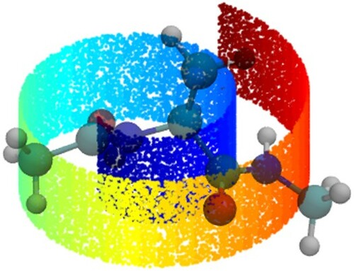
A second approach termed intrinsic map dynamics (iMapD) is due to Chiavazzo et al. [63]. Similar to DM-d-MD, short simulations are conducted and embedded using DMAPS. The boundary of this ‘intrinsic map’ is detected and extended outwards by a certain amount using local PCA. This step is critical to iMapD, as it involves the projection of points on the intrinsic manifold into unexplored regions, effectively allowing the system to tunnel through free energy barriers. Since the projected points may lie off-manifold, a lifting step is performed where the new configurations are restrained and the remaining degrees of freedom are relaxed. Once lifting is complete, new rounds of unbiased simulation are initialised from the projected boundary points and the procedure repeated until convergence. An illustration of the operation of iMapD is presented in Figure 3. An application of iMapD to computationally challenging simulations of the dissociation of the Mga2 dimer demonstrated its capacity to efficiently drive dissociation in just three iterations of the technique where millisecond-long unbiased simulations failed to do so [63]. Whereas DM-d-MD initialised new simulations at the frontier of the currently sampled phase space, iMapD performs a local extrapolation to seed new points beyond the current frontier, offering improved sampling efficiency and the possibility to tunnel through free energy barriers. The optimal size of the outward step can, however, be difficult to determine and, like DM-d-MD, the absence of artificial bias can impair barrier crossing efficiency.

Figure 3. Schematic illustration of iMapD. The curved teal sheet is a cartoon representation of a low-dimensional manifold residing within the high-dimensional coordinate space of the molecular system (black background) and to which the system dynamics are effectively restrained. This manifold supports the low-dimensional molecular free energy surface of system (red contours denote potential wells). The dimensionality of the manifold, good collective variables with which to parameterise it, and topography of the free energy surface are a priori unknown. iMapD commences by running short unbiased simulations to perform local exploration of the underlying manifold and which define an initial cloud of points $C^{(1)}$. Boundary points are identified, here $B{P}_1^{(1)}$ and $B{P}_2^{(1)}$, and local PCA applied to define a locally-linear approximation to the manifold geometry that is locally valid in the vicinity of each point. An outward step is then taken within these linear subspaces, here from $B{P}_1^{(1)}$ to expand the exploration frontier. The projected point may lie off the manifold due to the linear approximation inherent in the outward projection and so a short ‘lifting’ operation is employed to relax it back to the manifold. This point then seeds a new unbiased simulation that generates a new cloud of points $C^{(2)}$ and the process is repeated until the manifold is fully explored. In this manner iMapD explores the manifold by ‘walking on clouds’. Image adapted with permission from Ref. [63].

The application of artificial biasing potentials in the collective variables identified by DMAPS is made challenging by the absence of an explicit and differentiable mapping between the atomic coordinates and the DMAPS CVs. The out-of-sample extension techniques discussed in Section 2.2 furnish approximate projections for new data and enable energy biases to be applied in Monte-Carlo simulations as perturbations to the unbiased Hamiltonian conditioned on the current value of the DMAPS CVs [169–171]. The approximations introduced by these extrapolations, however, typically render them too numerically unstable for reliable derivative calculation and the implementation of force biases in molecular dynamics simulation. One solution to this problem is offered by the diffusion nets (DNETS) approach of Mishne et al., who train an ANN encoder to learn a functional map from the atomic coordinates to the low-dimensional DMAPS embeddings [172]. By construction, this map is both explicit and differentiable, opening the door to its use within off-the-shelf molecular dynamics enhanced sampling techniques such as umbrella sampling or metadynamics. The authors also train a ANN decoder to reconstruct molecular configurations from the DMAPS manifold, which may also be useful in ‘hallucinating’ new molecular configurations outside the currently explored phase space that may then be lifted and used to initialise new simulations in the mould of iMapD.

3.2. Smooth and nonlinear data-driven CVs (SandCV)

In a similar spirit to the DNETS approach of Mishne et al. (Section 3.1), Hashemian et al. developed an approach termed smooth and nonlinear data-driven collective variables (SandCV) to estimate explicit and differentiable expressions for CVs discovered by nonlinear dimensionality reduction and then apply bias in these CVs to perform enhanced sampling [39]. In principle, SandCV is compatible with any nonlinear dimensionality technique and enhanced sampling protocol, but it was originally developed to operate with Isomap [50] and adaptive biasing force (ABF) [173]. The heart of SandCV is estimation of the explicit and differentiable function $\mathcal{C}:\mathbf{r}\in {\mathbb{R}}^D\to \mathit{\xi }=\mathcal{C}(\mathbf{r})\in {\mathbb{R}}^d$ that projects a D-dimensional all-atom Cartesian configuration $\mathbf{r}$ into a point $\mathit{\xi }$ in the d-dimensional Isomap manifold, and d<<D. The mapping $\mathcal{C}(\mathbf{r})$ can be conceived of as the composition of three functional maps, (4) $\mathcal{C}(\mathbf{r})={\mathcal{M}}^{-1}\circ \mathcal{P}\circ \mathcal{A}(\mathbf{r}),$(4) as illustrated in Figure 4. $\mathcal{A}(\mathbf{r})$ performs alignment of the atomic configuration to (some subset of) the atoms $\mathbf{x}$ of a reference structure, $\mathcal{P}(\mathbf{x})$ performs a projection of the aligned configuration to the nearest neighbour point within the previously constructed Isomap manifold, and ${\mathcal{M}}^{-1}(\mathbf{x})$ performs projection of this point into the manifold and is itself the inverse of a function $\mathcal{M}(\mathit{\xi })$ that is a mapping from the points in the manifold back to the aligned molecular configurations achieved through a basis function expansion in a small number of landmark points. Enhanced sampling is effected by applying biasing forces over the manifold $\mathbf{F}(\mathit{\xi })$ and propagating these to forces on atoms $\mathbf{F}(\mathbf{r})$ through the Jacobian of the mapping function $\mathbf{D}\mathcal{C}(\mathbf{r})$. SandCV is demonstrated in applications to alanine dipeptide in vacuum and explicit water. In an instance of transfer learning, it is shown that data-driven CVs computed for a simpler system (alanine dipeptide in vacuum) can be applied to a more complex system (alanine dipeptide in water). In a followup publication, the authors propose an extension to SandCV that builds an atlas of locally-valid CVs that are subsequently stitched together, which can be valuable in parameterising complex free energy topologies where different regions of conformational space may require different CVs for their parameterisation [174].

Figure 4. Schematic illustration of SandCV. Molecular configurations $\mathbf{r}$ are aligned to a reference configuration $\mathcal{A}(\mathbf{r})$ then projected onto the Isomap manifold using a nearest neighbour projection and a basis function expansion in a number of landmark points ${\mathcal{M}}^{-1}\circ \mathcal{P}(\mathbf{x})$. Enhanced sampling using adaptive biasing force (ABF) is effected by propagating biasing forces over the manifold $\mathbf{F}(\mathit{\xi })$ into forces on atoms $\mathbf{F}(\mathbf{r})$ through the Jacobian of the explicit and differentiable composite mapping function $\mathcal{C}(\mathbf{r})={\mathcal{M}}^{-1}\circ \mathcal{P}\circ \mathcal{A}(\mathbf{r})$. Image reprinted from Ref. [39], with the permission of AIP Publishing.

SandCV relies on the availability of representative configurations covering the region of configurational phase space of interest since the projection of points onto the manifold is through projection onto nearest neighbours. When no such data are available, SandCV uses initial high-temperature simulations to provide seed configurations for the manifold learning. The subsequent enhanced sampling is then able to interpolatively bridge the gaps between the sparse initial landscape, but it remains undemonstrated as to whether the algorithm can extrapolatively drive sampling into new regions of configuration space.

3.3. Molecular enhanced sampling with autoencoders (MESA)

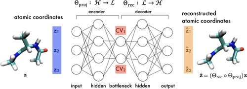
DNETS (Section 3.1) and SandCV (Section 3.2) furnish explicit and differentiable approximations linking the atomic coordinates to the low-dimensional CVs furnished by nonlinear dimensionality reduction, which can subsequently be used to conduct enhanced sampling. Chen et al. proposed an alternative nonlinear dimensionality approach based on deep learning that learns nonlinear CV that possess explicit and differentiable mappings by construction [37,64]. In doing so, the functional estimation step is eliminated and enhanced sampling may be conducted directly in the learned CVs without approximation error. This approach, termed molecular enhanced sampling with autoencoders (MESA), employs an deep neural network (DNN) with an autoencoding architecture or ‘autoencoder’ (AE) comprising an encoder ${\mathrm{\Theta }}_{\mathrm{proj}}:\mathbf{z}\in \mathcal{H}\to \mathit{\xi }\in \mathcal{L}$ that maps molecular configurations $\mathbf{z}$ in a high-dimensional coordinate space $\mathcal{H}$ to a nonlinear projection $\mathit{\xi }$ in a low-dimensional latent space $\mathcal{L}$, and a decoder ${\mathrm{\Theta }}_{\mathrm{rec}}:\mathit{\xi }\in \mathcal{L}\to \hat{\mathbf{z}}\in \mathcal{H}$ that approximates the reverse mapping (Figure 5). The network is trained to reconstruct its own inputs (i.e. autoencode) such that $\mathbf{z}\approx \hat{\mathbf{z}}$ and therefore discover a low-dimensional latent space $\mathit{\xi }$ defined by the ANN activations in a bottleneck layer that preserves the salient information necessary to perform an approximate reconstruction. The appropriate dimensionality of the latent space, and therefore number of nonlinear CVs required for reconstruction, can be tuned on-the-fly. Since the encoding $\mathit{\xi }={\mathrm{\Theta }}_{\mathrm{proj}}(\mathbf{z})$ is furnished by a ANN it is explicit and differentiable by construction and can be used to propagate biasing forces in the CVs $\mathbf{F}(\mathit{\xi })$ to forces on atoms $\mathbf{F}(\mathbf{z})$.

Figure 5. Molecular enhanced sampling with autoencoders (MESA). An autoencoding neural network (autoencoder) is trained to reconstruct molecular configurations via a low-dimensional latent space where the CVs are defined by neuron activations within the bottleneck layer. The encoder ${\mathrm{\Theta }}_{\mathrm{proj}}$ performs the low-dimensional projection from molecular coordinates $\mathbf{z}$ in the high dimensional atomic coordinate space $\mathcal{H}$ into the low-dimensional latent space $\mathcal{L}$ and the decoder ${\mathrm{\Theta }}_{\mathrm{rec}}$ performs the approximate reconstruction back to $\hat{\mathbf{z}}$. The encoder furnishes, by construction, an exact, explicit, and differentiable mapping from the atomic coordinates to CVs that can be modularly incorporated into any off-the-shelf CV biasing enhanced sampling technique.

To encourage complete sampling of phase space and improvement of the data-driven CVs, rounds of CV discovery and enhanced sampling are interleaved in an iterative framework comprising successive: (i) learning CVs from simulation trajectories (either the initial unbiased trajectory or biased trajectories obtained from previous iterations of CV biasing) and (ii) applying CV biasing with the learned CV to push the frontier outwards and drive exploration of new regions of phase space using umbrella sampling (but arbitrary CV biasing approaches may be employed). The process is terminated when CVs stabilise between successive rounds and the volume of phase space explores converges. Applications to alanine dipeptide and Trp-cage demonstrate the capacity of the technique to discover, sample, and determine free energy surfaces in nonlinear CVs starting from no prior knowledge of the system [37]. The iterative expansion of the frontier and refinement of CVs as a function of location in phase space is analogous to that in iMapD and DM-d-MD but the application of accelerating biasing forces greatly enhances barrier crossing. The use of the explicit and differentiable mapping to perform enhanced sampling is similar to SandCV but the mathematical framework enabled by ANNs is much simpler and the functional mapping is exact by construction. The use of biasing forces does, of course, corrupt the true dynamics of the system and so dynamical observables (e.g. Markov state models) cannot be straightforwardly extracted from the simulation data. A followup paper shows that tailoring the autoencoder architecture and error functions can help discover better CVs, improve sampling efficiency, and favour the discovery of more stable and interpretable CVs [64].

3.4. Reweighted autoencoded variational Bayes for enhanced sampling (RAVE)

Akin to MESA (Section 3.3), reweighted autoencoded variational Bayes for enhanced sampling (RAVE) due to Ribeiro et al. uses DNNs to learn nonlinear CVs for enhanced sampling [175]. It differs from MESA in that it makes use of variational autoencoders (VAEs) [122], seeks a 1D latent space encoding only the leading CV, and conducts sampling not directly in the discovered CV but in a proxy physical variable (or linear combinations thereof) that maximally resembles that of the CV. The use of VAEs compared to AEs conveys advantages in producing better regularised and continuous latent space embeddings. Identification of a physical variable χ in which to perform sampling is very attractive from an interpretability standpoint, but means sampling is necessarily performed in a proxy for the data-driven CV. The quality of the proxy variable in approximating the discovered CV is contingent on the space of candidate physical variables considered. The probability distribution in the optimal physical variable $P(\chi )$ is then turned into a biasing potential $V_{\mathrm{bias}}(\chi )=k_{B}T\ln P(\chi )$ from which, by virtue of the physical nature of χ for which an explicit relation to the atomic coordinates is known, is straightforwardly converted into biasing forces. An iterative procedure very similar to MESA is then applied to drive system exploration by interleaving rounds of biased simulation and CV learning.

The restriction to single CVs is limiting, but the framework can, in principle, be extended to multidimensional CVs. One way to do so may be to employ β-VAEs to encourage independence of the various CVs [176,177], but an alternative approach is adopted in an extension of the framework known as Multi-RAVE in which a set of locally valid one-dimensional CVs are constructed and the piecewise sum of these position-dependent components is a single-nonlinear CVs spanning relevant configurational space [178]. Numerical experiments with the disassociation of benzene from L99A lysozome predict unbinding free energies in good agreement with experiment.

3.5. Reinforcement learning based adaptive sampling (REAP)

The CVs parameterising configurational space may vary substantially as a function of location over that space. For example, those CVs appropriate to parameterise and enhance configurational sampling in the vicinity of the native fold of a protein may differ significantly from those appropriate for the unfolded ensemble, and protein activation frequently involves two (or more) distinct molecular events parameterised by different CVs that occur in series and result in characteristic ‘L-shaped’ landscapes. By maintaining a sufficiently large ensemble of CVs, one may determine on-the-fly which subset of CVs constitute the active space for enhanced sampling at any given location in phase space. This is the approach taken by reinforcement learning based adaptive sampling (REAP) introduced by Shamsi et al., which employs reinforcement learning (RL) to determine the relative importance of different candidate CVs as a system explores phase space [36]. REAP proceeds by running an initial round of short molecular simulations. The resulting configurations are then clustered, the least-populated clusters identified, and a reward function measuring the normalised absolute distance from the ensemble mean evaluated for each candidate CV for each cluster. An optimisation problem is solved to maximise the overall reward function as a weighted sum of the candidate CVs, and the clusters that offer the highest rewards selected as those from which to harvest configurations to seed a new round of simulations. This process is repeated until sufficient sampling of the phase space is achieved. The key feature of any RL approach is the reward function, which in the case of REAP is designed to maximise discovery of new conformational states. Like RAVE, the success of REAP is contingent on the quality and size of the space of candidate CVs. RL remains one of the less explored areas of ML in applications to molecular simulation, and it remains to be seen what advantages it can bring to adaptive sampling relative to the unsupervised approaches discussed in Sections 3.1–3.4.

3.6. Determining collective variables through supervised learning

Supervised learning is also relatively under-explored in molecular CV discovery relative to unsupervised techniques since the output variables (a.k.a. dependent variables, labels) for which we wish to construct a model in terms of our input variables (a.k.a. independent variables, descriptors, features) are often not obvious or available. Sultan and Pande recently proposed that the (pre-defined) metastable states of a molecular system may be adopted as output variables and supervised learning deployed to construct a pairwise or one-vs-all decision function to discriminate between the states and serve as a CV for enhanced sampling [179]. Such a situation may arise in protein activation where crystal structures for the active and inactive states are available but the activation pathway and mechanism is unknown. The supervised learning task is cast as a classification problem taking as input the atomic coordinates of the molecule in the various states and output as the labels of the states, and which is solved by support vector machines (SVM), logistic regression, and ANNs. The resulting decision function – distance to separating hyperplane for SVM, probability or odds ratio for logistic regression, unnormalised network output for ANN – provides an explicit and differentiable CV that is deployed in metadynamics simulations to drive sampling between states. The approach is demonstrated in applications to alanine dipeptide and chignolin, where it is shown to effectively drive reactive transitions [179]. Success of the approach is predicated on prior knowledge of the relevant states, and, like path sampling, the decision function CVs are inherently interpolative and so can have difficulty driving sampling into unexplored regions of phase space.

Mendels et al. independently developed harmonic linear discriminant analysis (HLDA) and multi class HLDA (MC-HLDA) as a supervised learning approach based on a generalisation of Fisher's linear discriminant [180,181]. The method takes as input the means and covariance matrices within a predefined set of descriptors for K metastable states as measured by short molecular simulations. An optimisation problem is formulated to find the $(K-1)$ linear projections within the descriptor space that maximise the ratio between the between-state and within-state scatter matrices, which corresponds to maximisation of a Fisher ratio and can be solved via a generalised eigenvalue problem. The linear projections within the descriptor space furnish CVs in which to perform metadynamics enhanced sampling. An application to chignolin demonstrates that the method successfully generates reactive pathways between the folded and unfolded states, although the efficiency of the approach can be sensitive to the user-defined selection of descriptors [182]. Again, this approach requires prior knowledge of the relevant metastable states, and is not designed to drive sampling into new configurational states.

3.7. Transfer operator theory and variational approaches to conformational dynamics

The CV discovery approaches discussed thus far have largely sought to discover high-variance CVs within the configurational phase space using some form of unsupervised, supervised, or reinforcement learning. We now proceed to discuss some recent developments in the data-driven discovery of slow (i.e. maximally autocorrelated) CVs that can often be more mechanistically meaningful and provide superior coordinates for the direct acceleration of the slowest dynamical processes. The theoretical foundations for the determination of these CVs is founded in spectral analysis of the transfer operator that propagates probability distributions over molecular microstates through time [84,85,88,106,162,163]. In an important theoretical development, Noé and Nuske showed that the spectral analysis of the operator can be performed in a data-driven fashion within the variational approach to conformational dynamics (VAC) in the case of equilibrium systems [84,85] or variational approach to Markov processes (VAMP) in the case of non-reversible and non-stationary dynamics [80,81]. These frameworks possess a pleasing parallel with the variational approach to approximate electronic wavefunctions within a given basis set through solution of the quantum mechanical Roothan-Hall equations [183,184]. Full details of the VAC and VAMP can be found in Refs. [80,81,84,85,88,106,185]. Here we briefly survey a number of recently developed machine learning approaches for slow CV discovery that seek to perform data-driven diagonalisation of the transfer operator.

As discussed in Section 2.4, TICA adopts as a basis set a featurization $\mathit{\xi }(\mathbf{x})$ of the atomic coordinates $\mathbf{x}$ (in the original TICA formulation $\mathit{\xi }(\mathbf{x})=\mathbf{x}$) and solves a generalised eigenvalue problem (Equation (3(3) ${\mathbf{C}}_{\tau }\mathbf{U}={\mathbf{C}}_0\mathbf{U}\mathbf{\Lambda },$(3) )) to define maximally autocorrelated linear projections within this basis. Kernel TICA (kTICA) is a generalisation of the TICA algorithm described in Section 2.4 that employs the kernel trick to apply the TICA machinery within a nonlinear transformation of the feature space [88]. The nonlinearity of the kernel function provides kTICA with greater expressive power, and the capacity to learn nonlinear slow modes from time-series data with higher fidelity than TICA [88]. As is typical of kernel-based methods, kTICA is computationally expensive and sensitive to kernel selection and hyperparameter choice [88, 89, 106, 110].

Time-lagged autoencoders (TAE) approximate slow CVs by performing nonlinear time-lagged regression using deep learning. Applied in the context of molecular simulation by Wehmeyer and Noé, TAEs employ an autoencoder architecture in which the encoder maps a configuration ${\mathbf{z}}_t$ at time t to a latent encoding ${\mathbf{e}}_t$, and the decoder maps ${\mathbf{e}}_t$ to a time-lagged output ${\mathbf{z}}_{t+\tau }=D({\mathbf{e}}_t)$ that minimises the time-lagged reconstruction loss to the true time-lagged configuration $\mathcal{L}=\mathbb{E}\left[{\Vert D({\mathbf{e}}_t)-{\mathbf{z}}_{t+\tau }^{\mathrm{true}}\Vert }^2\right]$ [108] (Figure 6). The underlying principle of operation is that minimisation of this time-lagged reconstruction loss promotes the discovery of slow CVs as the latent space variables ${\mathbf{e}}_t$ [109]. The technique is demonstrated in applications to alanine dipeptide and villin protein, and is shown to perform favourably against TICA, particularly when suboptimal molecular featurizations are employed.

Figure 6. Block diagram of a time-lagged autoencoder (TAE). The encoder projects a molecular configuration ${\mathbf{z}}_t$ at time t into a low-dimensional latent embedding ${\mathbf{e}}_t$ from which a time-lagged molecular configuration ${\mathbf{z}}_{t+\tau }$ at time $(t+\tau )$ is subsequently reconstructed. For τ = 0 the TAE reduces to a standard AE and the CV discovery process is equivalent to MESA (Section 3.3). Image reprinted from Ref. [108], with the permission of AIP Publishing.

Variational dynamics encoders (VDEs) are a deep learning approach for slow CV discovery first introduced by Hernández et al. [110]. VDEs employ a similar DNN autoencoding architecture as TAEs, but differ in their use of a VAE, as opposed to a standard AE, and a mixed loss function, (5) $\mathcal{L}=\lambda (\mathbb{E}\left[{\Vert D({\mathbf{e}}_t)-{\mathbf{z}}_{t+\tau }\Vert }^2\right]+L_{KL})-(1-\lambda )A({\mathbf{e}}_t),$(5) where $\mathbb{E}\left[{\Vert D({\mathbf{e}}_t)-{\mathbf{z}}_{t+\tau }\Vert }^2\right]$ is the time-lagged reconstruction loss, $A({\mathbf{e}}_t)$ is the autocorrelation of the learned 1D latent space CV ${\mathbf{e}}_t$, $L_{KL}$ is a regularisation term that measures the similarity of the distribution of ${\mathbf{e}}_t$ in the latent space to a Gaussian distribution, and $0\le \lambda \le 1$ is a linear mixing parameter [109]. In an application to the folding of villin protein, VDEs were shown to outperform TICA in the discovery of CVs capable of resolving metastable states and that the VDE latent coordinates produced superior MSMs with slower implied timescales [110].

TAEs and VDEs possess two key limitations. First, they are restricted to the discovery of 1D latent spaces and cannot be applied to learn multiple hierarchical slow modes due to the absence of orthogonality constraints in latent space [109]. Second, the incorporation of the time-lagged reconstruction loss within the loss function compromises the ability of the networks to discover the highly autocorrelated (i.e. slow) modes at the expense of high-variance modes [109]. In general, TAEs and VDEs discover mixtures of maximum variance modes and slow modes [109].

State-free reversible VAMPnets (SRVs) solve both of the deficiencies of TAEs and VDEs for equilibrium systems by employing a variational minimisation of a loss function that maximises the VAMP-2 (or more generally VAMP-r) score measuring the cumulative kinetic variance explained within the subspace of data-driven slow CVs [106]. The VAMP-2 score can be interpreted as the squared sum of the exponentials of the implied timescales of the slow CVs discovered by SRVs, and is guaranteed by the VAC to reach a maximum when the approximated slow CVs are coincident with the true slow CVs of the transfer operator [20,81,162]. SRVs can be conceived of as an application of TICA in which DNNs are employed to learn optimal nonlinear featurizations of the atomic coordinates as a learned basis set that is subsequently passed to the generalised eigenvalue problem (Equation (3(3) ${\mathbf{C}}_{\tau }\mathbf{U}={\mathbf{C}}_0\mathbf{U}\mathbf{\Lambda },$(3) )) [106]. The idea of learning an optimal basis to pass to a linear variational approach was first proposed by Andrew et al. in the context of deep CCA [104] and first applied to molecular simulations in Mardt et al.'s VAMPnets [81].

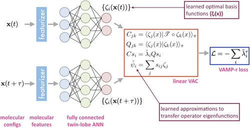
SRVs employ a twin-lobe neural network that transform pairs of time-lagged molecular configurations $\{\mathbf{x}(t),\mathbf{x}(t+\tau )\}$ into a space of d learned nonlinear basis functions $\{\mathit{\zeta }(\mathbf{x}(t)),\mathit{\zeta }(\mathbf{x}(t+\tau ))\}$ (Figure 7). These basis functions are passed to the linear VAC where solution of the generalised eigenvalue problem furnishes approximations to the transfer operator eigenfunctions as orthogonal linear projections within this basis. The key to the entire approach is the definition of the negative VAMP-r score as a loss function under which the twin-lobed ANN is iteratively trained to learn the nonlinear basis within which linear approximations of the d leading transfer operator eigenfunctions $\tilde{\mathit{\psi }}=\{{\psi }_1,{\psi }_2,\dots ,{\psi }_d\}$ are computed. Once trained, the ANN and generalised eigenvalue problem define an explicit and differentiable mapping between the atomic coordinates and slow CVs that can be straightforwardly deployed in CV biasing enhanced sampling routines [106]. SRVs have been demonstrated in applications to alanine dipeptide, WW domain, and Trp-cage, and proven to be a simple, efficient, and robust means for slow CV determination that possesses strong theoretical guarantees [106,107]. Moreover, SRVs have been shown to present an excellent and modular replacement for TICA within MSM construction pipelines. The nonlinear SRV latent space presents a kinetically superior latent space for microstate clustering than the linear embeddings furnished by TICA, with the resulting MSMs exhibiting faster implied timescale convergence and higher kinetic resolution than current state-of-the art approaches [107]. Replacement of the VAC within the SRV with the more general VAMP principle serves to extend the approach to non-stationary and non-reversible processes resulting in the more general state-free non-reversible VAMPnets (SNRV).

Figure 7. State-free reversible VAMPnets. Pairs of time-lagged molecular configurations $\{\mathbf{x}(t),\mathbf{x}(t+\tau )\}$ are featurized and transformed by a twin-lobe ANN into a space of nonlinear basis functions $\{\mathit{\zeta }(\mathbf{x}(t)),\mathit{\zeta }(\mathbf{x}(t+\tau ))\}$. These basis functions are employed within a linear VAC to furnish approximations $\tilde{\mathit{\psi }}$ to the leading eigenfunctions of the transfer operator. The twin-lobed ANN is trained to maximise a VAMP-r score measuring the cumulative kinetic variance explained and which reaches a maximum when the eigenfunction approximations are coincident with the true eigenfunctions of the transfer operator.

3.8. Deep learning based MSMs

Noé and co-workers recently proposed two variants of MSMs based on deep learning: VAMPnets [81] and deep generative MSMs (DeepGenMSM) [135]. SRVs (Section 3.7, Figure 7) were inspired by VAMPnets and both approaches share a similar twin-lobe network architecture to apply deep CCA [81,104,106]. They differ in two main respects. First, whereas SRVs pass these basis functions to a VAC analysis that is appropriate for approximating the transfer operator eigenfunctions for equilibrium data, VAMPnets pass them to a more general VAMP analysis to approximate the transfer operator singular functions for non-stationary and non-reversible data [81,105]. Second, whereas it is the goal of SRVs to furnish approximations to the leading modes of the transfer operator, it is the goal of VAMPnets to offer an end-to-end replacement for the entire MSM pipeline of featurization, dimensionality reduction, clustering, and kinetic model construction [81]. Integration of these steps within a single framework can be advantageous in helping to avoid the extensive parameter tuning that can plague the various steps in MSM model construction (Section 2.3). VAMPnets achieve this goal by employing softmax activations in the terminal layer of the twin ANN lobes that map a time-lagged pair of molecular configurations $\{{\mathbf{x}}_t,{\mathbf{x}}_{t+\tau }\}$ to fuzzy state assignments $({\mathit{\chi }}_0({\mathbf{x}}_t),{\mathit{\chi }}_1({\mathbf{x}}_{t+\tau }))$, where ${\mathit{\chi }}_0$ and ${\mathit{\chi }}_1$ are k-dimensional vectors defined over the k softmax output nodes of the two ANN lobes, and which assign a probability that the molecular configuration should be assigned to one of k metastable macrostates. The instantaneous and time-lagged covariance matrices ${\mathbf{C}}_{00}=\mathbb{E}[{\mathit{\chi }}_0({\mathbf{x}}_t){\mathit{\chi }}_0({\mathbf{x}}_t{)}^{\mathrm{T}}]$ and ${\mathbf{C}}_{01}=\mathbb{E}[{\mathit{\chi }}_0({\mathbf{x}}_t){\mathit{\chi }}_1({\mathbf{x}}_{t+\tau }{)}^{\mathrm{T}}]$ are then computed and used to estimate the MSM transition matrix between states $\mathbf{K}={\mathbf{C}}_{00}^{-1}{\mathbf{C}}_{01}$ [81]. VAMPnets are illustrated in an application to NTL9 where they discovers a 5-state model with kinetic properties on par with a 40-state conventional MSM, thereby illustrating the value of the approach in furnishing more parsimonious, efficient, and interpretable models without compromising kinetic accuracy [81].

DeepGenMSMs are a deep learning approach to not only learn a MSM defined by a discrete transition matrix between metastable states, but also a means to generate realistic molecular trajectories including previously unseen configurations not included in the training data [105,135]. DeepGenMSMs are based on the following representation of the transition density between a configuration $({\mathbf{x}}_t=\mathbf{x})$ at time t and $({\mathbf{x}}_{t+\tau }=\mathbf{z})$ at time $(t+\tau )$, (6) $\begin{array}{rl}\mathbb{P}({\mathbf{x}}_{t+\tau }& =\mathbf{z}|{\mathbf{x}}_t=\mathbf{x})=\mathit{\chi }(\mathbf{x}{)}^{\mathrm{T}}\mathbf{q}(\mathbf{z};\tau )\\ & =\sum _{i=1}^m{\chi }_i(\mathbf{x})q_i(\mathbf{z};\tau ),\end{array}$(6) where $\mathit{\chi }(\mathbf{x})=[{\chi }_1(\mathbf{x}),\dots ,{\chi }_m(\mathbf{x})]$ is a normalised vector representing the probability that configuration $\mathbf{x}$ exists within each of the $i=1\cdots m$ metastable macrostates, $\mathbf{q}(\mathbf{z};\tau )=[q_1(\mathbf{z};\tau ),\dots ,q_m(\mathbf{z};\tau )]$ is the vector of ‘landing densities’ where $q_i(\mathbf{z};\tau )=\mathbb{P}({\mathbf{x}}_{t+\tau }=\mathbf{z}|{\mathbf{x}}_t\in \mathrm{state}i)$ defines the probability that a system in macrostate i at time t lands in molecular configuration $\mathbf{z}$ at time $(t+\tau )$. The membership probabilities $\mathit{\chi }(\mathbf{x})$ and landing densities $\mathbf{q}(\mathbf{z};\tau )$ are learned by training a two-lobe ANN architecture similar to VAMPnets to maximise the likelihood of time-lagged pairs $({\mathbf{x}}_t,{\mathbf{x}}_{t+\tau })$ observed in simulation trajectories (Figure 8). The MSM transition matrix $\mathbf{K}$ between the m metastable states is furnished by the ‘rewiring trick’ wherein $\mathbf{K}=\mathbb{E}[\mathbf{q}(\mathbf{x};\tau )\mathit{\chi }(\mathbf{x}{)}^{\mathrm{T}}]$. In order to generate molecular configurations outside of the training data, it is additionally necessary to train a generator to sample from the density specified by the learned landing densities $\mathbf{q}(\mathbf{z};\tau )$, (7) $G(i,ϵ;\tau )=\mathbf{y}\sim q_i(\mathbf{y};\tau ),$(7) where i indexes over the states and ε is i.i.d. random noise sampled from a Gaussian distribution that powers the generator. Applications of DeepGenMSM to alanine dipeptide demonstrate its ability to accurately estimate the long-time kinetics and stationary distributions and also generate molecularly realistic structures including in regions of phase space where no training data was supplied [135].

Figure 8. Deep Generative MSM (DeepGenMSM) and the ‘rewiring trick’. (left) The encoder $\mathit{\chi }(\mathbf{x})$ within the twin-lobe ANN is trained to learn mappings of molecular configurations $\mathbf{x}$ to probabilistic memberships $\mathbf{y}$ of one of m macrostates. The generator is trained against the learned ‘landing probabilities’ $q_i(\mathbf{z};\tau )$ that a system prepared in macrostate i will transition to molecular configuration $\mathbf{z}$ after a time τ. (right) The rewiring trick reconnects the generator and encoder to furnish a valid estimate $\tilde{\mathbf{K}}$ for the MSM transition matrix between the embedding into the m discrete states learned by the encoder. Image adapted from Ref. [135], with permission from the author Prof. Frank Noé (Freie Universität Berlin).

3.9. Software

We list in Table 1 software packages and libraries implementing some of the CV discovery and enhanced sampling methods discussed in this review.

Table 1. Software packages and libraries available for some of the collective variable discovery and enhanced sampling techniques discussed in this review.

Method	Software Packages
ANNs	Keras (keras.io)
	TensorFlow (www.tensorflow.org)
	PyTorch (pytorch.org)
DMAPS	github.com/hsidky/dmaps
	github.com/DiffusionMapsAcademics/ pyDiffMap
MSM, TICA	PyEmma (www.emma-project.org/latest/)
	MSMBuilder (msmbuilder.org/)
MESA	github.com/weiHelloWorld/accelerated_ sampling_with_autoencoder
TAE, VAMPnets	github.com/markovmodel/deeptime
VDE	github.com/msmbuilder/vde
SRV	github.com/hsidky/srv
DeepGenMSM	github.com/markovmodel/deep_gen_msm
Enhanced Sampling Suites	SSAGES (github.com/MICCoM/SSAGES-public)
	PLUMED (www.plumed.org)
	Colvars (colvars.github.io)

4. Conclusion and outlook

It has been the goal of this review to offer a survey of some of the most exciting recent developments and applications of machine learning to collective variable discovery and enhanced sampling in biomolecular simulation. We sought to expose the essence of each method, its advantages and drawbacks, the systems in which it has been applied and demonstrated, and the availability of software implementations. We close with a retrospective assessment of the key milestones in the field and our outlook on emerging challenges and opportunities.

The origins of machine learning for CV discovery can be traced back to pioneering applications of linear dimensionality reduction techniques in the early 1990s. The first major development arrived in the early 2000s with the debut of powerful nonlinear dimensionality reduction tools. The mid-2000s witnessed the emergence of MSMs in the field. The late 2000s and early 2010s saw the introduction of techniques focussed on the discovery of slow as opposed to high-variance CVs. Advances in the past several years have been propelled in large part by deep learning methodologies coming to the fore. ANNs themselves are, of course, not a new idea, with roots dating back to Rosenblatt's perceptron in 1958 [186], but the availability of fast simulation codes (e.g. Gromacs, HOOMD, LAMMPS, NAMD, OpenMM), cheap storage, inexpensive high-performance GPU hardware, and user-friendly neural network libraries (e.g. PyTorch, TensorFlow, Keras) created ideal conditions for this flare of creative new applications and has supercharged the field. There has been a tandem development of enhanced sampling techniques for accelerated sampling of configurational space. Umbrella sampling is one of the earliest techniques that is still in use today [152] and which is itself based on ideas some 10 years prior by McDonald and Singer [187]. There has been an enormous proliferation of techniques since that time, based on a variety of approaches to enhance sampling [188]. Metadynamics [23], itself based on ideas from local elevation [189] and conformational flooding [190], has emerged as one of the most popular, flexible, and robust enhanced sampling techniques [191]. Enhanced sampling approaches have also benefited from the proliferation of deep learning technologies, and there are now a number of examples of ANN-based approaches to build biasing potentials for enhanced sampling [124–128].

Looking forward, we see a number of new frontiers and important challenges for machine learning-enabled CV discovery and enhanced sampling. First, with relatively few exceptions, many of the new tools are developed and tested for relatively small systems, and tend not to be tested in applications to larger systems. Of course it is vital to validate new tools in testbed problems where the ground truth is known a priori, but demonstrating the efficacy of these approaches in applications to large biomolecules of technological, biological, or biomedical import is crucial in proving their potential in the context of impactful and challenging problems.

Second, applications of these approaches tend to focus on single protein molecules (e.g. peptide folding, membrane protein activation). There are very good reasons for this privileging of protein folding from historical – the protein folding problem is a long-standing and alluring challenge [192,193] – biological – there are unquestionably critical problems in protein folding of great biological, biotechnological, and therapeutic value [194,195] – and practical – the best-validated computational force fields and experimental crystal structures are available for proteins – perspectives, but there are also compelling and important problems in related areas such as peptide assembly, peptoid engineering, and nucleic acid folding. It is important to develop methods in the context of diverse applications since it is not always the case that methods developed for proteins may be directly transferable and must be adapted to the specific vicissitudes of each system. For example, peptoid amide bonds occupy both cis and trans configurations (in contrast to those of peptides that are almost exclusively trans) but the transitions between them is a notoriously high-free energy barrier rare event [196]. To paraphrase the Persian poet Ibn Yamin (1286–1367), these slow CVs are ‘known unknowns’ and CV discovery and acceleration must explicitly account for these effects to achieve good sampling and enable CV discovery to identify the ‘unknown unknowns’.

Third, recent years have witnessed the convergence of CV discovery and enhanced sampling into integrated frameworks that are not beholden to the initial choice of CVs, but perform iterative CV refinement in tandem with accelerated phase space exploration either through judicious initialisation of unbiased simulations [44,58, 63] or the direct application of artificial bias [37,64]. These approaches have only been demonstrated for high-variance CVs, and it remains to demonstrate these iterative strategies for slow CVs. In the case of the unbiased sampling, the challenge is to recover estimates of CVs for the equilibrium system from many short non-equilibrium runs, which may be possible using Koopman reweighting [79]. In the case of biased sampling, the challenge is to estimate unbiased CVs from biased trajectories, which may be possible using Girsanov reweighting [65,66]. It may also be beneficial to ‘deflate’ out undesired slow modes [197].

Fourth, the field can benefit from two current waves in machine learning that have come to be referred to as eXplainable Artificial Intelligence (XAI) and Physics-aware Artificial Intelligence (PAI) [198,199]. The degree of interpretability that we require of our CVs is largely a matter of context and taste: interpretability may not be a primary concern if our CVs are simply viewed as a means to enhance sampling, but it may be extremely desirable if we wish to understand mechanisms or learn transferable CVs appropriate for larger classes of systems. One way to achieve interpretability is to use simple (usually linear) models that are interpretable by construction (e.g. linear regression, linear SVMs), but frequently we wish to exploit the power and flexibility of modern tools (e.g. ANNs) without sacrificing interpretability. Very recently developed XAI tools such as layer-wise relevance propagation offer a means to achieve this goal and simultaneously detect and avoid so-called ‘clever Hans’ solutions that formulate a seemingly correct answer but for the wrong reasons [200,201]. PAI seeks to incorporate physical constraints and knowledge into the CV discovery process, and is an extremely attractive for many reasons: the machine learning algorithms are given a ‘warm start’ by build upon prior understanding and knowledge of the system, the algorithms can function more robustly and work with noisier and smaller quantities of data since the model space is physically constrained, discovered CVs may be made more transferable to related systems, and the CV predictions can be guaranteed to satisfy particular physical constraints. PAI has proven somewhat difficult to realise in a generalisable way, but there have been recent successes in particular applications [202]. The rigorous enforcement of particular constraints and symmetries can be attractive in guaranteeing that the discovered CVs are consistent with the invariances, equivariances, and symmetries of the physical system (e.g. translational invariance, permutational invariance, rotational equivariance, energy conservation) [203,204].

Fifth, in a similar vein to PAI it can be valuable to incorporate experimental constraints within the CV discovery process. One may wish to promote CVs consistent with some physical prior knowledge (e.g. burial of hydrophobic residues, known tertiary contact pairs) or ensemble averages over the sampled phase space should be consistent with measured experimental observables. Unlike hard physical constraints that should be rigorously obeyed, it is likely that these experimental constaints may be incorporated in a softer manner through, for example, regularising Bayesian priors [205].

Sixth, the implementation and dissemination of open-source software and libraries implementing the CV discovery and sampling methods is critical in lowering the barrier to adoption by new users, guaranteeing reproducibility, promoting transparency, enabling community development and collaboration, and offering valuable pedagogical materials for new entrants into the field. The rising popularity of user-friendly Jupyter notebooks (https://jupyter.org/) and repository hosting sites such as GitHub (https://github.com) and Bitbucket (https://bitbucket.org/) has made code sharing simpler and easier than ever, and there are encouraging trends that doing so is becoming a cultural norm within the field.

In closing, we see many exciting and innovative challenges and opportunities on the horizon for this fast moving field, and we look forward to the exciting new developments that are sure to emerge in the coming years.

Disclosure statement

A.L.F. is a consultant of Evozyne and a co-author of US Provisional Patents 62/853,919 and 62/900,420.

Additional information

Funding

This work was supported by MICCoM (Midwest Center for Computational Materials), as part of the Computational Materials Science Program funded by the U.S. Department of Energy, Office of Science, Basic Energy Sciences, Materials Sciences and Engineering Division, and by the National Science Foundation under Grant No. CHE-1841805. H.S. acknowledges support from the National Science Foundation Molecular Software Sciences Institute (MolSSI) Software Fellows program (Grant No. ACI-1547580) [206,207].

References

- D. Frenkel and B. Smit, Understanding Molecular Simulation: From Algorithms to Applications (Academic Press, San Diego, 2001).
- E.H. Lee, J. Hsin, M. Sotomayor, G. Comellas and K. Schulten, Structure 17 (10), 1295–1306 (2009).
- P.S. de Laplace, Introduction to Oeuvres, Vol. VII, Theorie Analytique de Probabilites (Gauthier-Villars, Paris, 1812).
- B. Alder and T. Wainwright, J. Chem. Phys. 27 (5), 1208–1209 (1957).
- B.J. Alder and T.E. Wainwright, J. Chem. Phys. 31 (2), 459–466 (1959).
- F.F. Abraham, R. Walkup, H. Gao, M. Duchaineau, T.D. De La Rubia and M. Seager, Proceedings of the National Academy of Sciences 99 (9), 5777–5782 (2002).
- F.F. Abraham, R. Walkup, H. Gao, M. Duchaineau, T.D. De La Rubia and M. Seager, Proc. Natl. Acad. Sci. 99 (9), 5783–5787 (2002).
- N. Tchipev, S. Seckler, M. Heinen, J. Vrabec, F. Gratl, M. Horsch, M. Bernreuther, C.W. Glass, C. Niethammer, N. Hammer, B. Krischok, M. Resch, D. Kranzlmüller, H. Hasse, H.J. Bungartz and P. Neumann, Int. J. High Perform. Comput. Appl. 33 (5), 838–854 (2019).
- D.E. Shaw, P. Maragakis, K. Lindorff-Larsen, S. Piana, R.O. Dror, M.P. Eastwood, J.A. Bank, J.M. Jumper, J.K. Salmon, Y. Shan and W. Wriggers, Science 330 (6002), 341–346 (2010).
- K. Lindorff-Larsen, S. Piana, R.O. Dror and D.E. Shaw, Science 334 (6055), 517–520 (2011).
- F. Noé, Biophys. J. 108 (2), 228 (2015).
- M. Karplus and G.A. Petsko, Nature 347 (6294), 631–639 (1990).
- C. Abrams and G. Bussi, Entropy 16 (1), 163–199 (2013).
- Y. Miao and J.A. McCammon, Mol. Simul. 42 (13), 1046–1055 (2016).
- C. Chipot and A. Pohorille, Free Energy Calculations (Springer, Berlin, 2007).
- J. Wang and A.L. Ferguson, Mol. Simul. 44 (13-14), 1090–1107 (2018).
- R.J. Allen, C. Valeriani and P.R. ten Wolde, J. Phys. 21 (46), 463102 (2009).
- E.E. Borrero and F.A. Escobedo, J. Chem. Phys. 127 (16), 164101 (2007).
- C. Wehmeyer, M.K. Scherer, T. Hempel, B.E. Husic, S. Olsson and F. Noé, Living J. Comput. Mol. Sci. 1 (1), 5965 (2018).
- B.E. Husic and V.S. Pande, J. Am. Chem. Soc. 140 (7), 2386–2396 (2018).
- J. Rogal, W. Lechner, J. Juraszek, B. Ensing and P.G. Bolhuis, J. Chem. Phys. 133 (17), 174109 (2010).
- A. Laio and M. Parrinello, Proc. Natl. Acad. Sci. 99 (20), 12562–12566 (2002).
- A. Laio and F.L. Gervasio, Rep. Prog. Phys. 71 (12), 126601 (2008).
- O. Valsson, P. Tiwary and M. Parrinello, Annu. Rev. Phys. Chem. 67, 159–184 (2016).
- S. Singh, M. Chopra and J.J. de Pablo, Annu. Rev. Chem. Biomol. Eng. 3 (1), 369–394 (2012).
- A. Ma and A.R. Dinner, J. Phys. Chem. B 109 (14), 6769–6779 (2005).
- S.B. Kim, C.J. Dsilva, I.G. Kevrekidis and P.G. Debenedetti, J. Chem. Phys. 142 (8), 02B613_1 (2015).
- F. Noé, A. Tkatchenko, K.R. Müller and C. Clementi, arXiv preprint arXiv:1911.02792 (2019).
- A.L. Ferguson, J. Phys. 30 (4), 043002 (2018).
- N.E. Jackson, M.A. Webb and J.J. de Pablo, Curr. Opin. Chem. Eng. 23, 106–114 (2019).
- K.T. Butler, D.W. Davies, H. Cartwright, O. Isayev and A. Walsh, Nature 559 (7715), 547–555 (2018).
- M.A. Rohrdanz, W. Zheng and C. Clementi, Annu. Rev. Phys. Chem. 64, 295–316 (2013).
- P. Tiwary and B.J. Berne, Proc. Natl. Acad. Sci. 113 (11), 2839–2844 (2016).
- M.M. Sultan and V.S. Pande, J. Chem. Phys. 149 (9), 094106 (2018).
- Z. Shamsi, K.J. Cheng and D. Shukla, arXiv preprint arXiv:1710.00495 (2017).
- W. Chen and A.L. Ferguson, J. Comput. Chem. 39 (25), 2079–2102 (2018).
- G.A. Tribello, M. Ceriotti and M. Parrinello, Proc. Natl. Acad. Sci. 109 (14), 5196–5201 (2012).
- B. Hashemian, D. Millán and M. Arroyo, J. Chem. Phys. 139 (21), 12B601_1 (2013).
- A.L. Ferguson, J. Comput. Chem. 38 (18), 1583–1605 (2017).
- A.L. Ferguson, A.Z. Panagiotopoulos, P.G. Debenedetti and I.G. Kevrekidis, Proc. Natl. Acad. Sci.107 (31), 13597–13602 (2010).
- A.L. Ferguson, A.Z. Panagiotopoulos, I.G. Kevrekidis and P.G. Debenedetti, Chem. Phys. Lett. 509 (1), 1–11 (2011).
- W. Zheng, M.A. Rohrdanz and C. Clementi, J. Phys. Chem. B 117 (42), 12769–12776 (2013).
- J. Preto and C. Clementi, Phys. Chem. Chem. Phys. 16 (36), 19181–19191 (2014).
- T. Ichiye and M. Karplus, Proteins 11 (3), 205–217 (1991).
- A.E. García, Phys. Rev. Lett. 68 (17), 2696 (1992).
- S.T. Roweis and L.K. Saul, Science 290 (5500), 2323–2326 (2000).
- Z. Zhang and J. Wang, 2006, in Proceedings of the 19th International Conference on Neural Information Processing Systems, pp. 1593–1600.
- P. Das, M. Moll, H. Stamati, L.E. Kavraki and C. Clementi, Proc. Natl. Acad. Sci. 103 (26), 9885–9890 (2006).
- J.B. Tenenbaum, V. De Silva and J.C. Langford, Science 290 (5500), 2319–2323 (2000).
- K.Q. Weinberger and L.K. Saul, Int. J. Comput. Vis. 70 (1), 77–90 (2006).
- C.G. Li, J. Guo, G. Chen, X.F. Nie, and Z. Yang, 2006, in 2006 International Conference on Machine Learning and Cybernetics, pp. 3201–3206.
- J. Wang, Geometric Structure of High-Dimensional Data and Dimensionality Reduction (Springer, Berlin, 2011).
- D.L. Donoho and C. Grimes, Proc. Natl. Acad. Sci. 100 (10), 5591–5596 (2003).
- M. Belkin and P. Niyogi, 2002, in Advances in Neural Information Processing Systems, pp. 585–591.
- A.L. Ferguson, A.Z. Panagiotopoulos, P.G. Debenedetti and I.G. Kevrekidis, J. Chem. Phys. 134 (13), 04B606 (2011).
- R.R. Coifman and S. Lafon, Appl. Comput. Harmon. Anal. 21 (1), 5–30 (2006).
- M.A. Rohrdanz, W. Zheng, M. Maggioni and C. Clementi, J. Chem. Phys. 134 (12), 03B624 (2011).
- M. Ceriotti, G.A. Tribello and M. Parrinello, Proc. Natl. Acad. Sci. 108 (32), 13023–13028 (2011).
- M. Ceriotti, G.A. Tribello and M. Parrinello, J. Chem. Theory Comput. 9 (3), 1521–1532 (2013).
- L.v.d. Maaten and G. Hinton, J. Mach. Learn. Res. 9 (Nov), 2579–2605 (2008).
- G.a. Tribello, M. Ceriotti and M. Parrinello, Proc. Natl. Acad. Sci. 107 (41), 17509–17514 (2010).
- E. Chiavazzo, R. Covino, R.R. Coifman, C.W. Gear, A.S. Georgiou, G. Hummer and I.G. Kevrekidis, Proc. Natl. Acad. Sci. 114 (28), E5494–E5503 (2017).
- W. Chen, A.R. Tan and A.L. Ferguson, J. Chem. Phys. 149 (7), 072312 (2018).
- L. Donati, C. Hartmann and B.G. Keller, J. Chem. Phys. 146 (24), 244112 (2017).
- L. Donati and B.G. Keller, J. Chem. Phys. 149 (7), 072335 (2018).
- J. Quer, L. Donati, B.G. Keller and M. Weber, SIAM J. Sci. Comput. 40 (2), A653–A670 (2018).
- H. Wu, F. Paul, C. Wehmeyer and F. Noé, Proc. Natl. Acad. Sci. 113 (23), E3221–E3230 (2016).
- J.D. Chodera, W.C. Swope, F. Noé, J.H. Prinz, M.R. Shirts and V.S. Pande, J. Chem. Phys. 134 (24), 06B612 (2011).
- J.H. Prinz, J.D. Chodera, V.S. Pande, W.C. Swope, J.C. Smith and F. Noé, J. Chem. Phys. 134 (24), 06B613 (2011).
- S. Klus, F. Nüske, P. Koltai, H. Wu, I. Kevrekidis, C. Schütte and F. Noé, J. Nonlinear Sci. 28 (3), 985–1010 (2018).
- S. Klus, P. Koltai and C. Schütte, arXiv preprint arXiv:1512.05997 (2015).
- M.O. Williams, C.W. Rowley and I.G. Kevrekidis, arXiv preprint arXiv:1411.2260 (2014).
- K.K. Chen, J.H. Tu and C.W. Rowley, J. Nonlinear Sci. 22 (6), 887–915 (2012).
- C.W. Rowley, I. Mezić, S. Bagheri, P. Schlatter, and D.S. Henningson, 2010, in Seventh IUTAM Symposium on Laminar-Turbulent Transition, pp. 43–50.
- M.S. Hemati, C.W. Rowley, E.A. Deem and L.N. Cattafesta, Theor. Comp. Fluid Dyn. 31 (4), 349–368 (2017).
- M.O. Williams, M.S. Hemati, S.T. Dawson, I.G. Kevrekidis and C.W. Rowley, IFAC-PapersOnLine 49 (18), 704–709 (2016).
- M.O. Williams, I.G. Kevrekidis and C.W. Rowley, J. Nonlinear Sci. 25 (6), 1307–1346 (2015).
- H. Wu, F. Nüske, F. Paul, S. Klus, P. Koltai and F. Noé, J. Chem. Phys. 146 (15), 154104 (2017).
- H. Wu and F. Noé, arXiv preprint arXiv:1707.04659 (2017).
- A. Mardt, L. Pasquali, H. Wu and F. Noé, Nat. Commun. 9 (1), 5 (2018).
- S. Hanke, S. Peitz, O. Wallscheid, S. Klus, J. Böcker and M. Dellnitz, arXiv preprint arXiv:1804.00854 (2018).
- S. Peitz and S. Klus, Automatica 106, 184–191 (2019).
- F. Noé and F. Nuske, Multiscale. Model. Simul. 11 (2), 635–655 (2013).
- F. Nüske, B.G. Keller, G. Pérez-Hernández, A.S.J.S. Mey and F. Noé, J. Chem. Theory Comput. 10 (4), 1739–1752 (2014).
- G. Pérez-Hernández, F. Paul, T. Giorgino, G. De Fabritiis and F. Noé, J. Chem. Phys. 139 (1), 07B604_1 (2013).
- C.R. Schwantes and V.S. Pande, J. Chem. Theory Comput. 9 (4), 2000–2009 (2013).
- C.R. Schwantes and V.S. Pande, J. Chem. Theory Comput. 11 (2), 600–608 (2015).
- M.P. Harrigan and V.S. Pande, bioRxiv p. 123752 (2017).
- J.H. Tu, C.W. Rowley, D.M. Luchtenburg, S.L. Brunton and J.N. Kutz, arXiv preprint arXiv:1312.0041 (2013).
- M.S. Hemati, M.O. Williams and C.W. Rowley, Phys. Fluids 26 (11), 111701 (2014).
- J.L. Proctor, S.L. Brunton and J.N. Kutz, SIAM J. Appl. Dyn. Syst. 15 (1), 142–161 (2016).
- J.N. Kutz, S.L. Brunton, B.W. Brunton and J.L. Proctor, Dynamic Mode Decomposition: Data-Driven Modeling of Complex Systems (SIAM, Philadelphia, 2016).
- J.N. Kutz, X. Fu and S.L. Brunton, SIAM J. Appl. Dyn. Syst. 15 (2), 713–735 (2016).
- J.N. Kutz, X. Fu, S.L. Brunton, and N.B. Erichson, 2015, in 2015 IEEE International Conference on Computer Vision Workshop (ICCVW), pp. 921–929.
- S. Klus, P. Gelß, S. Peitz and C. Schütte, Nonlinearity 31 (7), 3359 (2018).
- Q. Li, F. Dietrich, E.M. Bollt and I.G. Kevrekidis, Chaos 27 (10), 103111 (2017).
- M. Korda and I. Mezić, J. Nonlinear Sci. 28 (2), 687–710 (2018).
- H. Hotelling, Biometrika 28, 321–377 (1936).
- G. Froyland, Nonlinearity 12 (1), 79 (1999).
- J. Ding and A. Zhou, Physica D 92 (1–2), 61–68 (1996).
- S.M. Ulam, A Collection of Mathematical Problems, 8 vols. (Interscience Publishers, Geneva, 1960).
- G. Froyland, G.A. Gottwald and A. Hammerlindl, SIAM J. Appl. Dyn. Syst. 13 (4), 1816–1846 (2014).
- G. Andrew, R. Arora, J. Bilmes, and K. Livescu, 2013, in International Conference on Machine Learning, pp. 1247–1255.
- F. Noé, arXiv preprint arXiv:1812.07669 (2018).
- W. Chen, H. Sidky and A.L. Ferguson, J. Chem. Phys. 150 (21), 214114 (2019).
- H. Sidky, W. Chen and A.L. Ferguson, J. Phys. Chem. B 123 (123), 7999–8009 (2019).
- C. Wehmeyer and F. Noé, J. Chem. Phys. 148 (24), 241703 (2018).
- W. Chen, H. Sidky and A.L. Ferguson, J. Chem. Phys. 151, 064123 (2019).
- C.X. Hernández, H.K. Wayment-Steele, M.M. Sultan, B.E. Husic and V.S. Pande, Phys. Rev. E 97 (6), 062412 (2018).
- M.M. Sultan, H.K. Wayment-Steele and V.S. Pande, J. Chem. Theory Comput. 14 (4), 1887–1894 (2018).
- K.L. Priddy and P.E. Keller, Artificial Neural Networks: An Introduction, 68vols. (SPIE Press, Bellingham, 2005).
- M.H. Hassoun, Fundamentals of Artificial Neural Networks (MIT Press, Cambridge, MA, 1995).
- T. Chen and H. Chen, IEEE Trans. Neural Netw. 6 (4), 911–917 (1995).
- R. Hecht-Nielsen, Neural Networks for Perception (Elsevier, Amsterdam, 1992). pp. 65–93.
- L. Bottou, Neural Networks: Tricks of the Trade (Springer, Berlin, 2012). pp. 421–436.
- D.P. Kingma and J. Ba, arXiv preprint arXiv:1412.6980 (2014).
- A. Krizhevsky, I. Sutskever, and G.E. Hinton, 2012, in Advances in Neural Information Processing Systems, pp. 1097–1105.
- Y. LeCun, P. Haffner, L. Bottou and Y. Bengio, Shape, Contour and Grouping in Computer Vision (Springer, Berlin, 1999). pp. 319–345.
- I. Goodfellow, Y. Bengio and A. Courville, Deep Learning (MIT Press, Cambridge, MA, 2016).
- M.A. Kramer, AIChE J. 37 (2), 233–243 (1991).
- D.P. Kingma and M. Welling, arXiv preprint arXiv:1312.6114 (2014).
- I. Goodfellow, J. Pouget-Abadie, M. Mirza, B. Xu, D. Warde-Farley, S. Ozair, A. Courville and Y. Bengio, in Advances in Neural Information Processing Systems 27, edited by Z. Ghahramani, M. Welling, C. Cortes, N. D. Lawrence and K. Q. Weinberger (Curran Associates, Inc., Red Hook, 2014), pp. 2672–2680.
- H. Sidky and J.K. Whitmer, J. Chem. Phys. 148 (10), 104111 (2018).
- R. Galvelis and Y. Sugita, J. Chem. Theory Comput.13 (6), 2489–2500 (2017).
- E. Schneider, L. Dai, R.Q. Topper, C. Drechsel-Grau and M.E. Tuckerman, Phys. Rev. Lett. 119 (15), 150601 (2017).
- A.Z. Guo, E. Sevgen, H. Sidky, J.K. Whitmer, J.A. Hubbell and J.J. de Pablo, J. Chem. Phys. 148 (13), 134108 (2018).
- L. Bonati, Y.Y. Zhang and M. Parrinello, arXiv preprint arXiv:1904.01305 (2019).
- J. Behler and M. Parrinello, Phys. Rev. Lett. 98, 146401 (2007).
- R.Z. Khaliullin, H. Eshet, T.D. Kühne, J. Behler and M. Parrinello, Phys. Rev. B 81, 100103 (2010).
- Z. Li, J.R. Kermode and A. De Vita, Phys. Rev. Lett. 114, 096405 (2015).
- J. Wang, S. Olsson, C. Wehmeyer, A. Pérez, N.E. Charron, G. de Fabritiis, F. Noé and C. Clementi, ACS Cent. Sci. 5 (5), 755–767 (2019).
- F. Noé, S. Olsson, J. Köhler and H. Wu, Science 365 (6457), eaaw1147 (2019).
- D. Bhowmik, S. Gao, M.T. Young and A. Ramanathan, BMC Bioinformatics 19 (S18), 429 (2018).
- H. Wu, A. Mardt, L. Pasquali, and F. Noé, 2018, in Advances in Neural Information Processing Systems, pp. 3975–3984.
- E.N. Feinberg, D. Sur, Z. Wu, B.E. Husic, H. Mai, Y. Li, S. Sun, J. Yang, B. Ramsundar and V.S. Pande, ACS Cent. Sci. 4 (11), 1520–1530 (2018).
- K.T. Schütt, H.E. Sauceda, P.J. Kindermans, A. Tkatchenko and K.R. Müller, J. Chem. Phys. 148 (24), 241722 (2018).
- C.R. Qi, H. Su, K. Mo, and L.J. Guibas, 2017, in Proceedings of the IEEE Conference on Computer Vision and Pattern Recognition, pp. 652–660.
- R.S. DeFever, C. Targonski, S.W. Hall, M.C. Smith and S. Sarupria, Chem. Sci. 10 (32), 7503–7515 (2019).
- R.R. Coifman, S. Lafon, A.B. Lee, M. Maggioni, B. Nadler, F. Warner and S.W. Zucker, Proc. Natl. Acad. Sci. 102 (21), 7426–7431 (2005).
- A.W. Long and A.L. Ferguson, J. Phys. Chem. B 118 (15), 4228–4244 (2014).
- R.R. Coifman, Y. Shkolnisky, F.J. Sigworth and A. Singer, IEEE Trans. Image Process. 17 (10), 1891–1899 (2008).
- A.W. Long and A.L. Ferguson, Appl. Comput. Harmon. Anal. 47 (1), 190–211 (2019).
- J. Wang and A.L. Ferguson, Macromolecules 51 (2), 598–616 (2018).
- E.J. Nyström, Über die Praktische Auflösung von Linearen Integralgleichungen mit Anwendungen auf Randwertaufgaben der Potentialtheorie (Akademische Buchhandlung, Freiberg, 1929).
- N. Rabin and R.R. Coifman, 2012, in Proceedings of the 2012 SIAM International Conference on Data Mining, pp. 189–199.
- E. Chiavazzo, C. Gear, C. Dsilva, N. Rabin and I. Kevrekidis, Processes 2 (1), 112–140 (2014).
- B. Peters and B.L. Trout, J. Chem. Phys. 125 (5), 054108 (2006).
- B. Peters, G.T. Beckham and B.L. Trout, J. Chem. Phys. 127 (3), 034109 (2007).
- T. Berry, J.R. Cressman, Z. Greguric-Ferencek and T. Sauer, SIAM J. Appl. Dyn. Syst. 12 (2), 618–649 (2013).
- R.A. Mansbach and A.L. Ferguson, J. Chem. Phys. 142 (10), 03B607_1 (2015).
- G.M. Torrie and J.P. Valleau, J. Comput. Phys. 23 (2), 187–199 (1977).
- V.S. Pande, K. Beauchamp and G.R. Bowman, Methods 52 (1), 99–105 (2010).
- G.R. Bowman, V.S. Pande and F. Noé, An Introduction to Markov State Models and Their Application to Long Timescale Molecular Simulation, 797vols. (Springer Science & Business Media, Berlin, 2013).
- J.D. Chodera and F. Noé, Curr. Opin. Struct. Biol. 25, 135–144 (2014).
- J.H. Prinz, H. Wu, M. Sarich, B. Keller, M. Senne, M. Held, J.D. Chodera, C. Schütte and F. Noé, J. Chem. Phys. 134 (17), 174105 (2011).
- A.S. Mey, H. Wu and F. Noé, Phys. Rev. X 4 (4), 041018 (2014).
- F. Nüske, H. Wu, J.H. Prinz, C. Wehmeyer, C. Clementi and F. Noé, J. Chem. Phys. 146 (9), 094104 (2017).
- S. Röblitz and M. Weber, Adv. Data Anal. Classif.7 (2), 147–179 (2013).
- L. Molgedey and H.G. Schuster, Phys. Rev. Lett. 72 (23), 3634 (1994).
- T. Blaschke, P. Berkes and L. Wiskott, Neural. Comput. 18 (10), 2495–2508 (2006).
- F. Noé and C. Clementi, J. Chem. Theory Comput.11 (10), 5002–5011 (2015).
- F. Noé, R. Banisch and C. Clementi, J. Chem. Theory Comput. 12 (11), 5620–5630 (2016).
- G. Pérez-Hernández and F. Noé, J. Chem. Theory Comput. 12 (12), 6118–6129 (2016).
- K. Pearson, Lond. Edinb. Dubl. Phil. Mag. J. Sci. 2 (11), 559–572 (1901).
- H.J. Woo and B. Roux, Proc. Natl. Acad. Sci. 102 (19), 6825–6830 (2005).
- M.M. Sultan and V.S. Pande, J. Chem. Theory Comput. 13 (6), 2440–2447 (2017).
- J. McCarty and M. Parrinello, J. Chem. Phys. 147 (20), 204109 (2017).
- C.R. Laing, T.A. Frewen and I.G. Kevrekidis, Nonlinearity 20 (9), 2127 (2007).
- A.W. Long and A.L. Ferguson, Mol. Syst. Des. Eng. 3 (1), 49–65 (2018).
- Y. Ma and A.L. Ferguson, Soft. Matter 15 (43), 8808–8826 (2019).
- G. Mishne, U. Shaham, A. Cloninger and I. Cohen, Appl. Comput. Harmon. Anal. 1, 1–27 (2017).
- E. Darve, D. Rodríguez-Gómez and A. Pohorille, J. Chem. Phys. 128 (14), 144120 (2008).
- B. Hashemian, D. Millán and M. Arroyo, J. Chem. Phys. 145 (17), 174109 (2016).
- J.M.L. Ribeiro, P. Bravo, Y. Wang and P. Tiwary, J. Chem. Phys. 149 (7), 072301 (2018).
- I. Higgins, L. Matthey, A. Pal, C. Burgess, X. Glorot, M. Botvinick, S. Mohamed and A. Lerchner, ICLR 2 (5), 6 (2017).
- C.P. Burgess, I. Higgins, A. Pal, L. Matthey, N. Watters, G. Desjardins and A. Lerchner, arXiv preprint arXiv:1804.03599 (2018).
- J.M.L. Ribeiro and P. Tiwary, J. Chem. Theory Comput. 15 (1), 708–719 (2018).
- M.M. Sultan and V.S. Pande, arXiv preprint arXiv:1802.10510 (2018).
- D. Mendels, G. Piccini and M. Parrinello, J. Phys. Chem. Lett. 9 (11), 2776–2781 (2018).
- G. Piccini, D. Mendels and M. Parrinello, J. Chem. Theory Comput. 14 (10), 5040–5044 (2018).
- D. Mendels, G. Piccini, Z.F. Brotzakis, Y.I. Yang and M. Parrinello, J. Chem. Phys. 149 (19), 194113 (2018).
- D.J. Griffiths and D.F. Schroeter, Introduction to Quantum Mechanics (Cambridge University Press, Cambridge, 2018).
- A. Szabo and N.S. Ostlund, Modern Quantum Chemistry: Introduction to Advanced Electronic Structure Theory (Courier Corporation, Chelmsford, MA, 2012).
- M.K. Scherer, B.E. Husic, M. Hoffmann, F. Paul, H. Wu and F. Noé, arXiv preprint arXiv:1811.11714 (2018).
- F. Rosenblatt, Psychol. Rev. 65 (6), 386 (1958).
- I. McDonald and K. Singer, J. Chem. Phys. 47 (11), 4766–4772 (1967).
- Y.I. Yang, Q. Shao, J. Zhang, L. Yang and Y.Q. Gao, J. Chem. Phys. 151 (7), 070902 (2019).
- T. Huber, A.E. Torda and W.F. van Gunsteren, J. Comput. Aided Mol. Des. 8 (6), 695–708 (1994).
- H. Grubmüller, Phys. Rev. E 52 (3), 2893 (1995).
- A. Barducci, M. Bonomi and M. Parrinello, Wiley Interdiscip. Rev. Comput. Mol. Sci. 1 (5), 826–843 (2011).
- K.A. Dill, S.B. Ozkan, M.S. Shell and T.R. Weikl, Annu. Rev. Biophys.37, 289–316 (2008).
- K.A. Dill and J.L. MacCallum, Science 338 (6110), 1042–1046 (2012).
- G.A. Khoury, J. Smadbeck, C.A. Kieslich and C.A. Floudas, Trends Biotechnol. 32 (2), 99–109 (2014).
- N. Chennamsetty, V. Voynov, V. Kayser, B. Helk and B.L. Trout, Proc. Natl. Acad. Sci. 106 (29), 11937–11942 (2009).
- L.J. Weiser and E.E. Santiso, AIMS Mat. Sci. 4 (5), 1029–1051 (2017).
- B.E. Husic and F. Noé, J. Chem. Phys. 151 (5), 054103 (2019).
- A.L. Ferguson, ACS Cent. Sci. 4 (8), 938–941 (2018).
- W. Samek, Explainable AI: Interpreting, Explaining and Visualizing Deep Learning (Springer Nature, London, 2019).
- S. Bach, A. Binder, G. Montavon, F. Klauschen, K.R. Müller and W. Samek, PloS One 10 (7), e0130140 (2015).
- S. Lapuschkin, S. Wäldchen, A. Binder, G. Montavon, W. Samek and K.R. Müller, Nat. Commun. 10 (1), 60 (2019).
- T. Beucler, M. Pritchard, S. Rasp, P. Gentine, J. Ott and P. Baldi, arXiv preprint arXiv:1909.00912 (2019).
- M. Weiler, M. Geiger, M. Welling, W. Boomsma, and T. Cohen, 2018, in Advances in Neural Information Processing Systems, pp. 10381–10392.
- B. Anderson, T.S. Hy and R. Kondor, arXiv preprint arXiv:1906.04015 (2019).
- J.W. Pitera and J.D. Chodera, J. Chem. Theory Comput. 8 (10), 3445–3451 (2012).
- A. Krylov, T.L. Windus, T. Barnes, E. Marin-Rimoldi, J.A. Nash, B. Pritchard, D.G. Smith, D. Altarawy, P. Saxe, C. Clementi, T.D. Crawford, R.J. Harrison, S. Jha, V.S. Pande and T. Head-Gordon, J. Chem. Phys. 149 (18), 180901 (2018).
- N. Wilkins-Diehr and T.D. Crawford, Comput. Sci. Eng. 20 (5), 26–38 (2018).