A case study of density functional theory and domain-based local pair natural orbital coupled cluster for vibrational effects on EPR hyperfine coupling constants: vibrational perturbation theory versus ab initio molecular dynamics

Abstract

Local approximations of high-level ab initio methods make superior accuracy in the computation of molecular properties accessible by drastically decreasing computational times. As a consequence, these methods become applicable not only for large systems but also in schemes for which large numbers of calculations are necessary. In this work, we apply a recently developed open-shell implementation of the domain-based pair natural orbital coupled cluster singles doubles (DLPNO-CCSD) approach for the computation of vibrational corrections to the isotropic values of electron paramagnetic resonance (EPR) hyperfine coupling constants. We assess density functional theory (DFT) and DLPNO-CCSD approaches using two common but very different schemes: (1) vibrational perturbation theory based on equilibrium geometries, and (2) explicit canonical ensemble averages using configuration snapshots sampled from revPBE0-D3(0) ab initio molecular dynamics simulations. Both approaches are found to yield very similar results for the spin probe 2,2,3,4,5,5-hexamethylperhydroimidazol-1-oxyl (HMI) and are both feasible for systems of around 30 atoms. However, the numerical stability required for higher derivatives can become a limitation for local correlation methods in the case of vibrational perturbation theory.

GRAPHICAL ABSTRACT

Keywords:

• Electron paramagnetic resonance
• hyperfine coupling constants
• ab initio calculations
• vibrational corrections
• ab initio molecular dynamics

1. Introduction

For paramagnetic molecular systems, electron paramagnetic resonance (EPR) spectroscopy is an indispensable tool, as it allows one to obtain a detailed picture of the electronic structure of the compound, using the electronic spin as a sensitive probe [1]. The coupling of the electronic spin to the nuclear spins results in a fine structure of the EPR spectrum and is expressed in terms of the hyperfine coupling constant (HFCC), or A-tensor. While the A-tensor is a tensorial quantity, in liquid solution one typically only observes the isotropic components of the tensor (one third of its trace) due to rapid tumbling. The isotropic HFCC is a very local property that is directly related to the spin-density at the nucleus in question. Consequently, a detailed analysis of the potentially many HFCCs provides a detailed map of the spin distribution throughout the investigated system. Given the large amount of electronic structure information in HFCCs, their detailed and quantitative interpretation have been one of the most important goals in the quantum chemistry of EPR parameters. In fact, electronic structure simulations are often instrumental in developing the full information content of the observed spectra in terms of the systems geometric and electronic structure [2–4].

There are numerous benchmark studies in the literature that assess the accuracy of computational methods for HFCCs on a broad variety of systems. While in general, coupled cluster methods such as coupled cluster singles and doubles (CCSD) [5–10] or coupled cluster singles and doubles with perturbative triples (CCSD(T)) [11] are accepted as most robust and accurate but computationally demanding, double hybrid density functional theory (DFT) and standard hybrid DFT perform reasonably well. In particular, the ability to compute HFCCs using coupled cluster theory has been a significant step towards high accuracy for the interpretation and prediction of spectra and results at the CCSD or CCSD(T) level of theory typically yield quantitative accuracy [12–15]. Having essentially converged the accuracy of the electronic structure method reveals other shortcomings in the standard quantum chemical protocols that mostly rely on computing EPR properties using equilibrium structures. Notably, neglecting averaging effects due to vibrational motion as well as the impact of solvation prevents such calculations to reach ultimate overall accuracy relative to experimental data that are necessarily obtained at finite temperatures mostly in liquid or frozen solution.

Given this situation, the focus of the methodological investigations is currently shifting towards eliminating these sources of errors. For strongly geometry-dependent properties the most important missing contribution is often the vibrational motion of the nuclei. In fact, several detailed studies on small- to medium-sized organic radicals have demonstrated the importance of vibrational corrections to HFCCs. For some compounds, vibrational effects can account for as much as 50 $\mathrm{\%}$ of the HFCC [16–21]. Comparing results obtained at the DFT and coupled cluster levels of theory, Chen et al. even conclude that ‘···  the neglect of these corrections can lead to an artificially better agreement between the theoretical and experimental data, (··· ), that would hide real physical contributions to the HFCCs ’ [22]. Hence, it is now generally accepted that using sufficiently robust electron correlation methods and the inclusion of vibrational corrections can efficiently close the gap between experiment and theory for isolated molecules [23].

Many studies that include vibrational corrections have been carried out using perturbative schemes starting from the harmonic approximation, while another common approach is to evaluate ensemble averages using configuration snapshots that have been sampled from molecular dynamics trajectories. However, no matter whether perturbative approaches or sampling based on molecular dynamics is used to compute vibrational corrections, all such schemes obviously lead to a significant increase of the computational cost compared to a single-point calculation using some reference geometry. Hence, while both approaches have advantages and disadvantages, the application of high-level methods to vibrational corrections has so far been mostly limited to rather small systems.

When it comes to the underlying electronic structure method, the advent of local correlation approximations has alleviated the most prominent bottleneck of post-HF correlation methods, namely the high computational scaling with system size [24–31]. As a consequence, modern approximations for coupled cluster methods are now applicable in cases where a few years ago only DFT was available [32]. The ability to compute single-point energies and molecular properties very efficiently using local coupled cluster methods also allows these to be applied in schemes that do not require calculations on very large systems but require a large number of calculations. This includes the computation of HFCC, for which an efficient implementation has recently been reported in the framework of the domain-based local pair natural orbital approximation (DLPNO) to CCSD [33,34].

In this work, we apply DLPNO-CCSD calculations for the evaluation of vibrational corrections to isotropic HFCCs, $A_{\mathrm{iso}}$. In order to assess advantages and differences of different approaches, we follow two alternative strategies. On one hand, we use ab initio molecular dynamics (AIMD) [35] simulations to generate a canonical ensemble of snapshots of an important EPR probe molecule in the gas phase using a suitable hybrid functional, revPBE0-D3(0) and evaluate its EPR properties by performing single-point calculations on this set of configurations using both DLPNO-CCSD theory and the same hybrid DFT method. On the other hand, we apply second-order vibrational perturbation theory (VPT2) with DFT force fields (FFs) and property calculations at the DFT and DLPNO-CCSD level of theory. Note that ‘force field’ in the context of VPT refers to a Taylor expansion of the potential energy surface with respect to the molecular equilibrium structure (mostly obtained by using electronic structure theory such as hybrid DFT here), whereas the same term is used in the molecular dynamics community to denote the parameterised (molecular mechanics or MM) interaction potential. We compare both approaches and discuss the influence of sampling, the quality of the FF used for VPT2, and the relevance of using high-level electronic structure methods for molecular properties i.e. $A_{\mathrm{iso}}$ in the present case. Note that especially within perturbative approaches, numerical derivatives are typically used to compute the required higher-order FFs or property derivatives, which can cause problems for local correlation schemes [36] as will be discussed in detail.

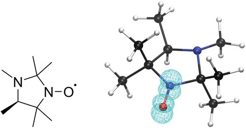
We focus the application of the different schemes on the 2,2,3,4,5,5-hexamethylperhydroimidazol-1-oxyl molecule, which we will simply denote as HMI in the following (see Figure 1). HMI provides a perfect test case with well characterised properties, high relevance for the experiment, and a size which renders the computations challenging for benchmarking. HMI belongs to a class of nitroxide radical spin labels which are widely used in EPR spectroscopic studies [37–42]. HMI itself is a pH-sensitive imidazole nitroxyl radical-based spin probe that has a variety of interesting properties and has been proposed, for example, for pH-monitoring inside chloroplasts [43,44]. It is well-known, that in such systems, the unpaired electron is mostly localised in a π* orbital involving the nitrogen in the 1 position and the adjacent oxygen with various degrees of delocalisation into the ring system depending on its chemical nature, in particular on the presence of conjugated double bonds.

Figure 1. Lewis structure and ball-and-stick representation of 2,2,3,4,5,5-hexamethylperhydroimidazol-1-oxyl (HMI) with the spin density (DLPNO-CCSD/def2-TZVPP-decS level of theory, iso-value=0.01) of the radical included in wireframe representation.

2. Theory

In order to assess advantages and drawbacks of both approaches for the computation of vibrational corrections to HFCCs, we shall first discuss some aspects of the theoretical background in the following before comparing them for the HMI molecule.

2.1. Second-order vibrational perturbation theory

The typical approach for perturbative vibrational corrections to molecular properties builds upon the harmonic approximation. A perturbative expansion yields a correction that depends on the cubic FF as well as the derivatives of the property in question with respect to all normal mode displacements.

Ruud et al. apply a perturbative treatment, using a cubic FF and effective reference geometries, to second-order properties such as chemical shieldings, magnetisabilities, and rotational g-tensors. They conclude that the approach is well suited for the computation of vibrational corrections to properties but can be sensitive to electron correlation effects [45]. Gauss and Stanton have applied a very similar approach, however based on equilibrium geometries ($R_e$) and VPT2 including a semi-numerical cubic FF and property derivatives. Several studies have shown that this scheme yields results in good agreement with related approaches and significantly increases the accuracy of high-level calculations in comparison to gas-phase experiments [46].

As we have adopted the latter approach in the following, we will reiterate the basic expressions of the VPT2 framework used to compute vibrational averages (see Equation 1(1) $\begin{array}{rl}⟨A⟩& =A_e+\sum _r{\left(\frac{\mathrm{\partial }A}{\mathrm{\partial }{Q}_r}\right)}_{Q_r=0}⟨Q_r⟩\\ & +\frac{1}{2}\sum _{r,s}{\left(\frac{{\mathrm{\partial }}^{2}A}{\mathrm{\partial }{Q}_r\mathrm{\partial }{Q}_s}\right)}_{Q_r,Q_s=0}⟨Q_r{Q}_s⟩\end{array}$(1) ) [47–49]. (1) $\begin{array}{rl}⟨A⟩& =A_e+\sum _r{\left(\frac{\mathrm{\partial }A}{\mathrm{\partial }{Q}_r}\right)}_{Q_r=0}⟨Q_r⟩\\ & +\frac{1}{2}\sum _{r,s}{\left(\frac{{\mathrm{\partial }}^{2}A}{\mathrm{\partial }{Q}_r\mathrm{\partial }{Q}_s}\right)}_{Q_r,Q_s=0}⟨Q_r{Q}_s⟩\end{array}$(1) (2) $\begin{array}{rl}⟨Q_r⟩& =\sqrt{\frac{1}{2\hslash {\omega }_r^3}}\sum _s{\varphi }_{\mathrm{rss}}\end{array}$(2) (3) $\begin{array}{rl}⟨Q_r{Q}_s⟩& ={\delta }_{\mathrm{rs}}\frac{\hslash }{4{\omega }_r}\end{array}$(3) The vibrational average of any given property $⟨A⟩$ can be evaluated by inclusion of two correction terms that appear in the same order of perturbation theory and are added to the property computed at the equilibrium geometry, $A_{\mathrm{e}}$. The first correction term depends on the derivative of the property and the expectation value of a normal mode displacement $⟨Q_r⟩$ with associated harmonic frequency ${\omega }_r$, which requires the evaluation of elements of the cubic FF φ (second term in Equation 1(1) $\begin{array}{rl}⟨A⟩& =A_e+\sum _r{\left(\frac{\mathrm{\partial }A}{\mathrm{\partial }{Q}_r}\right)}_{Q_r=0}⟨Q_r⟩\\ & +\frac{1}{2}\sum _{r,s}{\left(\frac{{\mathrm{\partial }}^{2}A}{\mathrm{\partial }{Q}_r\mathrm{\partial }{Q}_s}\right)}_{Q_r,Q_s=0}⟨Q_r{Q}_s⟩\end{array}$(1) and Equation 2(2) $\begin{array}{rl}⟨Q_r⟩& =\sqrt{\frac{1}{2\hslash {\omega }_r^3}}\sum _s{\varphi }_{\mathrm{rss}}\end{array}$(2) ). The second correction term consists of the second derivative of the property and the expectation value of the square normal mode displacement $⟨Q_r{Q}_s⟩$ which only requires the harmonic FF (Equation 3(3) $\begin{array}{rl}⟨Q_r{Q}_s⟩& ={\delta }_{\mathrm{rs}}\frac{\hslash }{4{\omega }_r}\end{array}$(3) ). Together, these two terms are denoted as the zero-point vibrational correction (ZPVC) of property A. The necessary property derivatives are typically evaluated by numerical differentiation using central finite differences. Note that in the well-established framework of perturbative treatments of vibrational corrections, these ZPVCs corresponding to the quantum vibrational ground state contribute the majority of the effects with respect to $R_{\mathrm{e}}$, while additional contributions due to the thermal population of excited vibrational quantum states and classical rigid-body rotation (collectively denoted as the ‘temperature correction’ (TC)) are found to be typically one order of magnitude smaller at room temperature [50,51]. Hence, the majority of vibrational effects should be captured by the ZPVCs from VPT2 considering only the quantum-mechanical ground vibrational state formally corresponding to 0 K.

In the present work, the harmonic FF and the molecular property are evaluated analytically, while the cubic FF and the property derivatives are evaluated by double-sided numerical differentiation. Hence, the calculation of the vibrational contribution to the HFCC of HMI, which has 87 vibrational degrees of freedom, requires 175 Hessian and HFCC calculations. It therefore becomes immediately obvious that a central aspect of computing vibrational corrections using VPT2 is to find a good compromise between obtaining accurate FF parameters and property values, and computational efficiency. Note that in the framework of VPT2, it is also possible to mix and match the level of theory for FF, property, and property derivatives easily. A combination of DFT and CCSD seems especially appealing in this case, as DFT typically yields fairly good results for force fields and CCSD is known for providing accurate results for HFCCs. However, perturbative approaches are limited to cases where anharmonicity can be considered a small perturbation with respect to some reference (e.g. equilibrium) geometry and cannot be applied to systems with soft degrees of freedom.

2.2. Ab initio molecular dynamics

Generation of sufficiently long trajectories by molecular dynamics (MD) propagation allows one to rigorously compute statistical-mechanical ensemble averages from the time averages of the respective observables computed along these trajectories if sampling has been ergodic. Thus, the usual microcanonical (NVE) simulations generate microcanonical averages, whereas proper thermostatting and barostatting at the desired temperature and pressure are required to generate the more relevant canonical (NVT) or isothermal-isobaric (NpT) thermal averages (according to Helmholtz or Gibbs free energies, respectively). An efficient way to easily generate such sufficiently long trajectories is to use pre-parameterised (a.k.a. MM) force fields in the framework of MD simulations. However, standard force fields are certainly not optimised to simulate open-shell species such as the vast set of spin probe molecules in particular.

An alternative to such pre-parameterised MD simulations is ab initio or AIMD simulations where the electronic structure problem is solved on-the-fly at each AIMD step, i.e. in conjunction with moving the nuclei using forces that have been computed based on analytical gradients [35]. Although AIMD is enormously more demanding compared to force field MD at the level of the computational effort, simulating molecules of the size of HMI in vacuum is routine if the interactions are computed from the generalised gradient approximation (GGA) to DFT. Unfortunately, GGA functionals are known to suffer from the self interaction error (SIE), which in effect leads to artificial spin-density delocalisation in case of open-shell species, possibly even beyond the molecule itself, for example into aqueous solution [52]. Various remedies have been introduced to counteract or fully cure the SIE, as shown in a pioneering study where an approximate self interaction correction has been applied to properly localise the unpaired electron [52]. Here, instead, we have opted to employ a specific hybrid functional without adjustment, namely revPBE0-D3(0) for reasons to be outlined below, to carry out the AIMD simulations of HMI.

3. Computational details

3.1. Single-point property calculations

All single-point property calculations on the AIMD snapshots and for the computation of the VPT2 corrections were done by means of the current development version of ORCA which is based on the released version ORCA 4.2 [53]. The def2-TZVPP basis set with decontracted s-functions was used [54] and TightSCF, convergence thresholds were applied for both levels of theory - revPBE0 and DLPNO-CCSD. For all calculations with revPBE0 a larger grid including an increased radial integral accuracy was chosen (Grid4, IntAcc 7). Note that the dispersion correction is excluded, as it does not contribute to the HFCC. The RIJK two-electron integral approximation with a decontracted auxiliary basis set (def2/JK) [55] for the calculation with revPBE0 whereas the correlation consistent auxiliary basis set with core polarisation functions (cc-pwCVTZ/C) [56] was used for the DLPNO-CCSD calculations and no approximation was used for the preceding HF calculation. For the DLPNO-CCSD HFCC computation, the settings for the construction and screening of PNOs had to be adjusted according to the Default2 setting resulting from the elaborate study on accurate DLPNO-CC spin densities for HFCCs by Saitow et. al. [34]

3.2. Second-order vibrational perturbation theory

For the perturbative approach, geometry optimisations, HFCC, and VPT2 calculations were carried out at several different levels of theory. All calculations in this section were performed with ORCA. For closest possible comparison with the AIMD results, the geometry was optimised at the revPBE0-D3(0)/def2-TZVPP level (without three-body dispersion terms, which is also the default in ORCA) [54,57,58]. Alternative optimisations were performed at the B97-3c [59], BP86-D3(BJ)/def2-TZVPP [54,60–62] and RI-MP2/cc-pVTZ[63–65], levels. The VeryTightOpt convergence settings were used, the RI approximation for Coulomb integrals (RI-J) was used with the def2/J fitting basis for the DFT calculations and the larger def2/JK for the RI-MP2 calculation [55,66], while the matching cc-pVTZ/C auxiliary basis set was used for the RI-MP2 approximation [67]. For B97-3c the default basis sets were used (def2-mTZVP and def2-mTZVP/J) [59]. Grid7 was used for BP86-D3(BJ) and revPBE0-D3(0) and Grid5 for B97-3c.

The Hessians for the VPT2 FFs were calculated using B97-3c and revPBE0-D3(0)/def2-TZVPP, starting from the respective optimised geometries. VeryTightSCF was chosen. For the latter method, the RIJCOSX approximation with dense grid settings (GridX8, %Method GridX 2) and a smaller DFT grid (Grid4 NoFinal Grid) were used [68]. This was found to introduce only minor deviations in the calculated vibrational frequencies, compared to the settings used for the optimisation (mean absolute deviation 0.2 cm${}^{-1}$, maximum 1.5 cm${}^{-1}$ or 0.6%), while speeding up the Hessian calculation by a factor of 10.

HFCC calculations at the optimised and displaced geometries were performed with revPBE0, RI-MP2, and DLPNO-CCSD, using the same settings as for the snapshot structures, except that an even larger integration grid was chosen (Grid6, IntAcc 7) to minimise numerical noise when calculating numerical derivatives. A step size of 0.05 in unitless normal coordinate displacements was used for numeric differentiation of both the force constants and the HFCCs. To confirm the stability of the results a second, larger step size (0.1 or 0.2) was used to evaluate the HFCC derivatives (see discussion below). We found that to achieve consistent results with both step sizes, it was necessary for some methods (RI-MP2 and revPBE0) to strictly enforce convergence of the density matrix elements during the SCF, using the flag ConvCheckMode=0.

3.3. Ab initio molecular dynamics and canonical averages of properties

For averaging the HFCCs of HMI based on MD snapshots, we have generated an ensemble of structures of a single HMI molecule in vacuum by means of Born–Oppenheimer AIMD simulations [35]. This means that the nuclei are propagated according to classical mechanics on the potential energy surface that is generated on-the-fly by unrestricted Kohn–Sham DFT in every step.

Due to the self interaction error in the GGA approach to DFT, widely used functionals in AIMD simulations such as PBE [69,70] or BLYP [71,72] are not good candidates for open-shell systems. Standard hybrid functionals, fortunately, are known to perform much more reliably in such cases since a proper admixture of nonlocal HF exchange on top of the semilocal GGA exchange approximately counteracts spin delocalisation artefacts. Specifically the PBE0 functional in conjunction with a suitable basis set ‘$\dots$ provides remarkably accurate magnetic properties at reasonable computational costs $\dots$’ [73] in vacuum (together with yielding the corresponding molecular equilibrium structures) as well as in aqueous solution [74]. Next, it has been found out that the revPBE0-D3 functional provides a very accurate description of the full-dimensional many-body potential energy surface for AIMD simulations of liquid bulk water as confirmed by adding nuclear quantum effects and comparing thereafter important observables to experimental data that quantify the structural, dynamical, and vibrational properties of water at ambient conditions [75].

Given these findings and having future applications to aqueous solutions in mind, as alluded to in the outlook, we have decided to use the hybrid version of a revised PBE functional, namely revPBE [57], along with the empirical D3 dispersion correction [58]. Here, following earlier work by others and us on liquid water [75,76] and aqueous solutions, [76] we only consider the two-body terms of the D3 correction and apply zero-damping in our present revPBE0-D3(0) AIMD simulations of HMI; note in the present context that all D3 terms are largely suppressed within small molecules such as HMI but that they will contribute in case of aqueous HMI solutions.

We have used the CP2K [77,78] package for the AIMD simulation. The bare HMI molecule was put inside a cubic box of dimension 15.9 Å and the electronic structure was solved using the Quickstep module [79,80] in CP2K, which uses an atom-centred Gaussian basis set to represent the Kohn–Sham orbitals, a plane-wave auxiliary basis set for the electron density and pseudo-potentials for core electrons. In the current study, we have employed the TZV2P Gaussian basis set in conjunction with Goedecker–Teter–Hutter (GTH) separable dual-space Gaussian pseudopotentials [81–83]. The auxiliary plane wave basis was truncated at a cutoff of 500 Ry. Since a single HMI molecule in vacuum is the system of current interest, the AIMD simulations were carried out using non-periodic cluster boundary conditions where the Poisson equation was solved using the CP2K wavelet scheme [84,85].

The simulations were performed in the NVT ensemble at 300 K as established by massive Nosé–Hoover chain (NHC) [86] thermostatting where every classical degree of freedom (meaning all three Cartesian coordinates of each atom) gets thermostatted individually by a separate NHC. A timestep of 0.5 fs was used to integrate the equations of motions to generate a trajectory for 54 ps, where the first 3 ps were sufficient to equilibrate the molecule given the usage of massive NHCs which are known to most efficiently and ergodically equipartition the kinetic energy even within stiff molecules such as HMI in vacuum. Thus, the remaining 51 ps of the trajectory were considered for extracting the canonical ensemble of snapshots to eventually compute EPR properties by single-point calculations. In order to compute the canonical averages of such properties, we have extracted snapshots from that thermalised trajectory every 200 fs as to provide largely uncorrelated configurations. These altogether 255 configurations were used subsequently to compute thermal averages from quantum-chemical property calculations.

4. Results and discussion

4.1. Calibration of electronic structure methods

In the following, we intend to study how DLPNO-CCSD calculations can be applied for the evaluation of vibrational corrections for molecular properties of open-shell species. But first, we need to assess how the choice of basis set, electronic structure method, and reference geometry affect the results for computed isotropic HFCCs.

We have chosen to use the def2-TZVPP [54] basis set for the computation of the HFCC of HMI after an extensive screening of Ahlrichs and Dunning basis sets including the def2 [54,87], cc-pVXZ [65], and cc-pCVXZ [88] families. Table 1 lists the HFCC values of N and O for def2-XVP(P) and cc-pCVXZ (X=S/D,T,Q) using the corresponding cc-pwCXZ/C auxiliary basis set and no frozen core approximation. Different contraction schemes were studied as given in the table for each basis set. As the HFCCs are very sensitive to the description of the core region, changes in the order of 2 and 6 MHz for nitrogen and oxygen, respectively, are observable when decontracting the triple-ζ basis set. For the double-ζ basis sets the change is much larger whereas for the quadruple-ζ basis sets the change is negligible. However, only small changes are observed when going from decontracting solely the s-functions (decS) to decontracting the whole basis set (decAll). Note that the cc-pCVTZ basis set already treats the core region more rigorously by including core polarisation basis functions. Therefore, the difference between the contracted and decontracted basis set is smaller for cc-pCVTZ ($\sim 0.6$ and 0.5 MHz) than for def2-TZVPP ($\sim 2.1$ and 6.7 MHz). Our results indicate that the residual basis set error at this level is smaller than 1 MHz, which renders the quality of the decontracted def2-TZVPP and cc-pCVTZ equally good for our purposes. The best efficiency is therefore obtained if the def2-TZVPP basis is employed and all s-functions are decontracted. We will denote this basis set as def2-TZVPP-decS in the following. Note that for the DLPNO-CCSD calculations it is absolutely essential to include all electrons in the correlation treatment as the HFCC includes operators like the Fermi-contact contribution, which emphasise the core region [89,90]. Hence, it is not surprising that using the frozen core approximation for CCSD, one essentially obtains the HF result: For the def2-TVZPP-decS basis set the corresponding DLPNO-CCSD result for the nitrogen HFCC is 61.13 MHz while the HF value is 59.96 MHz. In comparison to those values, the all-electron correlation treatment gives 30.09 MHz (see Tables 1 and 2).

Table 1. Dependence of the HFCCs of the nitroxy-N on the chosen basis set and decontraction scheme (decAll = decontraction of the whole basis set, decS = decontraction of the s-functions).

Basis set	Decontraction scheme	$A_{\mathrm{iso}}$(N) (MHz)	$A_{\mathrm{iso}}$(O) (MHz)
def2-SVP	Contracted	65.93	−164.89
	decS	25.81	−48.69
	decAll	25.37	−46.54
def2-TZVPP	Contracted	28.03	−49.26
	decS${}^{\mathrm{a}}$	30.09	−55.82
	decAll	30.11	−55.96
def2-QZVPP	Contracted	30.35	−54.73
	decS	30.25	−54.16
	decAll	30.43	−54.51
cc-pCVDZ	Contracted	24.70	−39.56
	decS	30.17	−56.12
	decAll	29.47	−53.78
cc-pCVTZ	Contracted	29.40	−55.70
	decS${}^{\mathrm{b}}$	30.00	−55.91
	decAll	30.04	−56.22
cc-pCVQZ	Contracted	30.57	−56.17
	decS	30.65	−55.91
	decAll	30.53	−56.61

Note: The calculations were done at DLPNO-CCSD level without the frozen core approximation and using the corresponding cc-pwCXZ/C auxiliary basis set (Geometry: revPBE0-D3(0)/def2-TZVPP.)

${}^{\mathrm{a}}$ Corresponding values (for N and O, respectively) with frozen core approximation: 61.13/–136.36 MHz, at HF-level: 59.96/–126.66 MHz, all-electron correlation treatment: 30.09/–55.82 MHz.

${}^{\mathrm{b}}$ Corresponding values with frozen core approximation: 59.92/–134.46 MHz, at HF-level: 58.93/–125.16 MHz, all-electron correlation treatment: 30.00/–55.91 MHz.

Table 2. Dependence of the HFCCs on the level of theory.${}^{\mathrm{a}}$

Method${}^{\mathrm{b}}$	$A{}_{\mathrm{iso}}(\mathrm{O})$ (MHz)	$A{}_{\mathrm{iso}}(\mathrm{N})$ (MHz)
HF	−126.66	59.96
revPBE	−21.25	18.85
revPBE0	−41.26	27.48
B3LYP	−41.88	26.67
TPSS	−32.29	23.64
TPSSh	−39.05	26.71
RI-MP2	−29.70	34.60
RI-SCS-MP2	−35.33	33.93
RI-DSD-BLYP	−50.76	32.57
RI-DSD-PBEP86	−48.27	31.91
DLPNO-CCSD	−55.82	30.09
DLPNO-CCSD frozen core	−136.36	61.13

${}^{\mathrm{a}}$ Geometry: revPBE0-D3(0)/def2-TZVPP.

${}^{\mathrm{b}}$ HFCC: def2-TZVPP-decS, cc-pwCVTZ/C (where applicable).

Table 2 summarises the computed values for the relevant nitrogen and oxygen atom in HMI at different levels of theory. In agreement with previous studies on the accuracy of results from DFT and post-HF methods, the treatment of electron correlation is the most important influence on the isotropic HFCCs. While the HF results deviate from all other results by more than 100$\mathrm{\%}$ and MP2 still shows significant deviations from the DLPNO-CCSD results, standard hybrid functionals like revPBE0 and B3LYP outperform both MP2 and SCS-MP2 and yield results reasonably close to CCSD, whereas related GGA functionals such as revPBE clearly fail. In contrast to MP2, double hybrid DFT methods actually yield results fairly close to the CCSD values. Thus, in what follows, we will employ mostly revPBE0 and DLPNO-CCSD (and MP2 for comparison) for computing vibrational corrections to the HFCCs in HMI. Note that for these methods, one has to account for deviations of more than 10 MHz between DFT and CCSD for oxygen and up to 3 MHz for nitrogen.

As we are going to compare vibrational corrections from a perturbative treatment based on a cubic FF and an average over snapshots of an AIMD simulation, the dependence of the property on the reference geometry in the former approach, e.g. the method that has been used to obtain the equilibrium geometry of the system, can yield an insight of how sensitive the property is to small changes in the structure. Table 3 summarises the results for isotropic HFCCs obtained at the revPBE0, RI-MP2, and DLPNO-CCSD levels of theory for different choices of reference geometries. From these, it becomes obvious that the results are fairly robust with respect to the reference geometry and the observed differences of up to 1 MHz are smaller than in the comparison of different electronic structure methods.

Table 3. Dependence of the HFCCs, calculated at different levels of theory, on the method used for geometry optimisation.

Geometry∖HFCC${}^{\mathrm{a}}$	revPBE0	RI-MP2	DLPNO-CCSD
$A{}_{\mathrm{iso}}(\mathrm{O})$ (MHz)
B97-3c	−41.27	−29.00	−56.01
BP86-D3(BJ)${}^{\mathrm{b}}$	−41.39	−29.00	−56.21
revPBE0-D3(0)${}^{\mathrm{b}}$	−41.26	−29.70	−55.82
RI-MP2${}^c$	−40.91	−28.94	−55.46
$A{}_{\mathrm{iso}}(\mathrm{N})$ (MHz)
B97-3c	27.61	35.94	30.17
BP86-D3(BJ)${}^{\mathrm{b}}$	28.14	37.02	30.70
revPBE0-D3(0)${}^{\mathrm{b}}$	27.48	34.60	30.09
RI-MP2${}^c$	26.76	33.60	29.37

${}^{\mathrm{a}}$ def2-TZVPP-decS, cc-pwCVTZ/C (where applicable).

${}^{\mathrm{b}}$ def2-TZVPP, RIJONX, def2/J.

${}^{\mathrm{c}}$ cc-pVTZ, cc-pVTZ/C, RIJONX, def2/JK.

From single-point calculations at equilibrium geometries we conclude that the level of theory applied for the computation of the HFCCs has a major influence, reference geometry effects are small, and the inclusion of core correlation is essential for post-HF schemes. Basis sets are sufficiently converged at the triple zeta level of theory, provided augmentation and/or decontraction of the basis sets in the core region to ensure sufficient flexibility for operators like in the Fermi-contact term.

4.2. Vibrational averages from VPT2

In order to be able to compare to the AIMD results, the VPT2 anharmonic FF was calculated with the same functional (revPBE0-D3(0)) and the def2-TZVPP basis set (which is similar but not strictly identical to the pseudopotential-based TZV2P-GTH basis that is used in these AIMD simulations). For comparison, the B97-3c method proposed by Grimme et al. was used, which combines a GGA functional with a ‘minimal’ triple-ζ basis set and semi-empirical corrections and represents a very cost-efficient approximation to full DFT treatments, such as revPBE0 [59,91]. Due to the lack of exact exchange and the smaller basis set, the analytic Hessian calculations with B97-3c were about 5 times faster than with revPBE0-D3(0). Different step sizes were used for the HFCC derivatives, in order to access the numerical stability of the results.

Results for the nitrogen and oxygen atoms are presented in Table 4. With the notable exception of DLPNO-CCSD, which will be discussed below, the ZPVCs do not change significantly when a different step size is used for the HFCC derivatives, which indicates they are numerically stable. There is also a decent agreement between the revPBE0 results (with both FFs) and the RI-MP2 ones, with ZPVCs in the range of 2.5–5.2 MHz for nitrogen and 0.5–0.8 MHz for oxygen. Out of the DLPNO-CCSD ZPVCs, the one obtained for nitrogen with a step size of 0.2 is the only one we consider reasonably accurate (for reasons discussed below), and it also falls in the same range at 3.5 MHz. This resembles what has been found for example for ZPVC of NMR shieldings -- it is often sufficient to evaluate the ZPVCs at a lower level of theory than the equilibrium property [92].

Table 4. Vibrational corrections to the HFCCs of HMI, calculated using VPT2 and different methods for the FF and HFCCs.

		Equilibrium		ZPVC		Total
FF	HFCC/step size	N	O	N	O	N	O
revPBE0-D3(0)${}^{\mathrm{a}}$	revPBE0${}^{\mathrm{b}}$/0.05	27.6	−41.1	2.5	0.5	30.1	−40.5
revPBE0-D3(0)${}^{\mathrm{a}}$	revPBE0${}^{\mathrm{b}}$/0.10			2.5	0.6	30.1	−40.5
revPBE0-D3(0)${}^{\mathrm{a}}$	RI-MP2${}^{\mathrm{c}}$/0.05	34.6	−29.7	5.3	0.8	39.9	−28.9
revPBE0-D3(0)${}^{\mathrm{a}}$	RI-MP2${}^{\mathrm{c}}$/0.10			5.2	0.8	39.8	−28.9
revPBE0-D3(0)${}^{\mathrm{a}}$	DLPNO-CCSD${}^{\mathrm{c}}$/0.05	30.1	−55.8	10.4	−7.4
revPBE0-D3(0)${}^a$	DLPNO-CCSD${}^{\mathrm{c}}$/0.20			3.5	−1.4	33.6
B97-3c	revPBE0${}^{\mathrm{b}}$/0.05	27.6	−41.3	3.4	0.6	31.0	−40.6
B97-3c	revPBE0${}^{\mathrm{b}}$/0.10			3.2	0.5	30.8	−40.8

Notes: All values in MHz. Total HFCCs are not given where the ZPVC is considered inaccurate (see text).

${}^{\mathrm{a}}$ def2-TZVPP, RIJONX, def2/J.

${}^{\mathrm{b}}$ def2-TZVPP-decS, RIJK, def2/JK.

${}^{\mathrm{c}}$ def2-TZVPP-decS, cc-pwCVTZ/C.

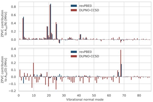
One advantage of the VPT2 approach is that it allows one to dissect the total ZPVCs of isotropic HFCCs in terms of the contributions due to the individual harmonic vibrational modes in the quantum ground state. HMI comprises 31 atoms and has 87 vibrational modes, so in total 175 Hessian and HFCC calculations are required to obtain the ZPVCs with VPT2. However, even for this relatively small molecule, not all normal modes have significant contributions to the corrections of the studied HFCCs (see Figure 2). For example, selecting the 20 normal modes with the largest contributions provides over 95% of the ZPVC for the nitrogen atom. From the figure, it is also apparent that the major ZPVC contributions to the nitrogen HFCC are in very good agreement between revPBE0 and DLPNO-CCSD (with a step size of 0.2 in the latter case). For the oxygen atom, the overall correction is an order of magnitude smaller and especially contributions which are very small at the revPBE0 level of theory appear to be very large at the DLPNO-CCSD level of theory. The source of this discrepancy will be investigated in the following paragraphs.

Figure 2. Contributions of each normal mode to the VPT2 ZPVCs of the nitrogen (top) and oxygen (bottom) HFCCs. A step size of 0.05 and 0.2 was used at the revPBE0 and DLPNO-CCSD levels, respectively. In both cases, the revPBE-D3(0) FF was used.

The fact that the DLPNO-CCSD ZPVCs in Table 4 change dramatically with the step size is a strong indication of numerical noise in the calculation of the HFCC derivatives. Recall that the latter are estimated using finite differences formulae, and are therefore very sensitive to small errors in the computed property. In order to pinpoint the source of these errors, we performed a series of HFCC calculations at displaced geometries along a single problematic normal mode of the revPBE0-D3(0) FF. The chosen mode is number 68, with a harmonic frequency of 1531 ${}^{-1}$, and is a combination of CH${}_3$ ‘scissoring’ and O–N stretching motions. At a step length of 0.05, the ZPVC contributions from this mode are $+0.78$ MHz for nitrogen and $-1.34$ MHz for oxygen with DLPNO-CCSD, and $-0.04$ MHz and $+0.18$ MHz, respectively, with revPBE0.

The additional results are given in Table 5. First, canonical CCSD calculations were performed with a smaller basis set, cc-pCVDZ-decS. The ZPVCs obtained from these are stable at different step sizes and in remarkable agreement with the revPBE0 results. The CCSD values with the fully contracted cc-pCVDZ basis were also practically identical, despite differences of ∼10 MHz in the absolute HFCCs. Hence, we consider these as reliable reference values, with which to compare the DLPNO-CCSD results. Note that the RI-MP2 ZPVC contributions for this mode are very different, which suggests that the total ZPVCs may only fortuitously be similar to the revPBE0 values.

Table 5. Comparison of ZPVC contributions from a single vibrational mode, calculated using different methods for the HFCCs, and different displacement step sizes.

HFCC method${}^{\mathrm{a}}$	Step	$A(0)$	$A(+x)$	$A(-x)$	ZPVC 1	ZPVC 2
$A_{\mathrm{iso}}(\text{N})$ (MHz)
DLPNO-CCSD${}^{\mathrm{b}}$	0.05	30.0925	30.1202	30.0724	0.02	0.76
	0.10		30.1404	30.0485	0.02	0.10
	0.15		30.1598	30.0276	0.02	0.03
	0.20		30.1714	30.0001	0.02	−0.08
	0.25		30.1876	29.9757	0.02	−0.09
DLPNO-CCSD+PNO${}^{\mathrm{c}}$	0.05	30.6543	30.6752	30.6294	0.02	−0.40
	0.10		30.6937	30.6074	0.02	−0.19
DLPNO-CCSD+DO${}^{\mathrm{d}}$	0.05	30.0914	30.1192	30.0703	0.02	0.67
	0.10		30.1394	30.0504	0.02	0.17
CCSD${}^{\mathrm{e}}$	0.05	32.0314	32.0656	31.9965	0.02	−0.08
	0.10		32.0991	31.9607	0.02	−0.08
revPBE0	0.05	27.5571	27.5707	27.5430	0.01	−0.05
	0.10		27.5838	27.5286	0.01	−0.04
RI-MP2	0.05	34.5783	34.1651	35.0042	−0.30	1.27
	0.10		33.7642	35.4434	−0.30	1.27
$A_{\mathrm{iso}}(\text{O})$ (MHz)
DLPNO-CCSD${}^{\mathrm{b}}$	0.05	−55.8170	−55.7931	−55.8545	0.02	−1.36
	0.10		−55.7611	−55.8803	0.02	−0.19
	0.15		−55.7231	−55.8831	0.02	0.31
	0.20		−55.6835	−55.8919	0.02	0.37
	0.25		−55.6487	−55.9135	0.02	0.29
DLPNO-CCSD+PNO${}^{\mathrm{c}}$	0.05	−56.2297	−56.1951	−56.2606	0.02	0.37
	0.10		−56.1611	−56.2891	0.02	0.23
DLPNO-CCSD+DO${}^{\mathrm{d}}$	0.05	−55.8192	−55.7952	−55.8635	0.02	−2.04
	0.10		−55.7637	−55.8822	0.02	−0.19
CCSD${}^{\mathrm{e}}$	0.05	−57.8043	−57.7845	−57.8226	0.01	0.16
	0.10		−57.7629	−57.8392	0.01	0.16
revPBE0	0.05	−41.0533	−41.0145	−41.0906	0.03	0.15
	0.10		−40.9742	−41.1263	0.03	0.15
RI-MP2	0.05	−29.6829	−29.7944	−29.5707	−0.08	0.06
	0.10		−29.9052	−29.4582	−0.08	0.06

Note: Given are the HFCCs at the equilibrium geometry ($A(0)$) and at positive and negative displacements along the normal mode ($A(+x)$ and $A(-x)$, respectively), as well as the first- and second-order contributions to the ZPVC (denoted ‘ZPVC 1’ and ‘ZPVC 2’).

${}^{\mathrm{a}}$ Unless otherwise noted: def2-TZVPP-decS, cc-pwCVTZ/C (where applicable). Geometry: revPBE0-D3(0)/def2-TZVPP.

${}^{\mathrm{b}}$ DLPNO-HFC2 thresholds.

${}^{\mathrm{c}}$ DLPNO-HFC2 thresholds with $T_{\mathrm{CutPNO}}={10}^{-9}$.

${}^{\mathrm{d}}$ DLPNO-HFC2 thresholds with $T_{\mathrm{CutDO}}={10}^{-3}$.

${}^{\mathrm{e}}$ cc-pCVDZ-decS.

Understandably, the biggest deviations in the DLPNO-CCSD results are in the second derivative contributions to the ZPVC, which are more sensitive to numerical noise. With increasing step size, the ZPVC changes sign and seems to converge at a step size of 0.2 (which is why it was chosen above) to a value close to the reference, especially for nitrogen. However, for oxygen, it is apparent that the larger step size does not result in a meaningful result for the total ZPVC, which shows that the remaining deviation at step size 0.2, for this and other modes, is still significant. Thus, it is not sufficient to decrease the denominator in the finite difference formula, but also the numerator, $A(+x)+A(-x)-2A(0)$, must be evaluated more precisely. Having confirmed sufficient convergence of the SCF and CCSD equations (see Supplemental Data), the obvious source of error in the DLPNO-CCSD calculations are the various local approximations, such as the domain and PNO truncations, controlled by the thresholds $T_{\mathrm{CutDO}}$ and $T_{\mathrm{CutPNO}}$, respectively, with values $5\times {10}^{-3}$ and ${10}^{-8}$ given by the DLPNO-HFC2 setting. 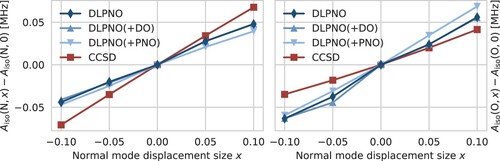Separately tightening them to $1\times {10}^{-3}$ and ${10}^{-9}$, respectively, results in the values denoted by ‘+DO’ and ‘+PNO’ in Table 5. Increasing the domain sizes has a minor effect on the HFCCs and does not improve the ZPVCs. On the other hand, tightening the PNO threshold has a larger effect and produces ZPVCs with the correct sign, although these are still not consistent between both step sizes. The changes of the HFCCs upon displacement are visualised in Figure 3. The first- and second-order ZPVCs are proportional to the first and second derivatives of the plotted curves. The kinks in the DLPNO and DLPNO(+DO) curves are visible, especially for the oxygen atom, while the DLPNO(+PNO) curves are noticeably smoother.

Figure 3. Change of the nitrogen (left) and oxygen (right) HFCC upon displacement along normal mode 68 (see text for details). Calculations performed with DLPNO-CCSD/def2-TZVPP-decS and DLPNO-HFC2 thresholds (denoted simply ‘DLPNO’), same with tighter $T_{\mathrm{CutDO}}={10}^{-3}$ (‘DLPNO(+DO)’) or with tighter $T_{\mathrm{CutPNO}}={10}^{-9}$ (‘DLPNO(+PNO)’), and canonical CCSD/cc-pCVDZ-decS (‘CCSD’).

It is important to note that the discontinuities in the DLPNO-CCSD HFCC surfaces are likely not due to the local approximations themselves but to the changes in the correlation domains, strong/weak pair lists, etc., upon distortion of the geometry. Tightening the thresholds does not remove the discontinuities, it only reduces their magnitude. A better approach would be to keep the correlation domains fixed upon displacement, as done by Werner and coworkers for numerical derivatives and potential energy surfaces using local correlation methods [93–95]. However, this requires rather significant code modifications and thus falls outside the scope of the current work.

4.3. Thermal averages based on AIMD simulations

From the revPBE0-D3(0)/TZV2P-GTH AIMD trajectory of a single HMI molecule in vacuum, a set of altogether 255 snapshot configurations, representing a statistical-mechanical sample in the canonical ensemble at 300 K, was extracted as described above and used to compute the classical canonical average of isotropic HFCCs as obtained from single-point electronic structure calculations in a post-processing mode. 85 subsets were created in order to monitor the convergence of the averaged values obtained from snapshot calculations by picking 3, 6, 9, $\dots$, 255 random snapshots out of the total amount of 255 snapshots. The average value and the corresponding standard deviation for each subset was then calculated. The required single-point property calculations were carried out for all snapshots at the revPBE0/def2-TZVPP-decS and DLPNO-CCSD/def2-TZVPP-decS level of theory. Note that revPBE0 and revPBE0-D3(0) single-point properties are identical since the D3 dispersion correction does not affect the electronic structure of a frozen configuration. Figure 4 depicts the convergence of the average value of the isotropic HFCC, $A_{\mathrm{iso}}$, for the nitrogen and oxygen atoms of HMI as a function of the number of snapshots considered in the average. In line with previous studies [96], the average values stabilise after considering roughly 100 configurations in the statistical sample and are practically converged beyond that, whereas less than 50 snapshots are clearly insufficient to compute trustworthy thermal averages even for a quasi-rigid molecule such as HMI.

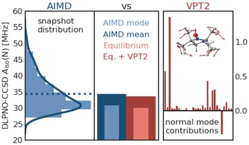
Figure 4. Convergence of the thermal averages of the isotropic HFCCs for the relevant nitrogen (left) and oxygen (right) atoms in HMI computed from single-point revPBE0 (top) and DLPNO-CCSD (bottom) property calculations shown as a function of the number of underlying configuration snapshots used to compute these averages. The snapshots have been extracted from the revPBE0-D3(0) AIMD simulation of HMI in vacuum in the canonical ensemble at 300 K, see text. The average values are shown as dots while the standard deviations given the respective sample size are shown as vertical lines. The red horizontal lines denote the final average using all 255 snapshots.

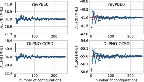
Figure 5 depicts a histogram of the distribution of the computed HFCCs from all snapshots. Interestingly, we observe that the maxima of the distributions (obtained as the modes of the depicted kernel density estimations) – corresponding to the most probable HFCC values – are with about $-41$ MHz (revPBE0) and $-56$ MHz (DLPNO-CCSD) for oxygen and 28 MHz (revPBE0) and 31 MHz (DLPNO-CCSD) for nitrogen very close to the values obtained when only using the equilibrium geometry, namely $-41$, $-56$, 27, and 30 MHz in that order. This is expected for a stiff quasi-rigid molecule, such as HMI, subject to only small-amplitude vibrations at the temperature of interest (to be analysed in significant detail in what follows below). Yet, the average isotropic HFCC value (see Figure 5), which is the experimental observable, can deviate from the corresponding most probable value, and thus from the equilibrium value, if the underlying canonical distribution function is sufficiently skewed as found here in case of $A_{\mathrm{iso}}$(N).

Figure 5. Histograms of the isotropic HFCCs for the relevant nitrogen (left) and oxygen (right) atoms in HMI computed from single-point revPBE0 (top) and DLPNO-CCSD (bottom) property calculations based on all configuration snapshots sampled from the revPBE0-D3(0) AIMD simulation of HMI in vacuum in the canonical ensemble at 300 K. The solid line displays the kernel density estimation curves which were used to determine the most probable $A_{\mathrm{iso}}$ values from the respective modes (upper value close to the maximum of each subplot), whereas the vertical dashed lines are the corresponding averages neither obtained from the histograms nor kernel densities approximations but on the full sample (lower value of each subplot), thus being identical to the red horizontal lines in Figure 4.

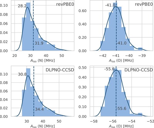
For the oxygen atom of HMI we reach converged average values of $-41.0$ MHz (revPBE0) and $-55.6$ MHz (DLPNO-CCSD). For the nitrogen atom in 1 position, the corresponding values are 31.9 MHz (revPBE0) and 34.4 MHz (DLPNO-CCSD). Note that the values obtained from single-point calculations using the revPBE0-D3(0) equilibrium geometry are $-41.3$ MHz (revPBE0) and $-55.8$ MHz (DLPNO-CCSD) for oxygen and 27.5 MHz (revPBE0) and 30.1 MHz (DLPNO-CCSD) for the nitrogen, respectively (see Table 3). Subtraction from the thermal averages yields correction values of 0.3 MHz (revPBE0) and 0.2 MHz (DLPNO-CCSD) for oxygen and 4.4 MHz (revPBE0) and 4.3 MHz (DLPNO-CCSD) for nitrogen, respectively. These are what we call the ‘thermal fluctuations corrections’ (TFCs) which transform the isotropic HFCC values computed based on a single property calculation at the equilibrium geometry, $A_{\mathrm{iso}}(R_{\mathrm{e}})$, to the corresponding thermal average at the desired temperature, ${⟨A_{\mathrm{iso}}⟩}_{>T}$, which is the observable that should better be compared to experimental data.

4.4. Comparison of VPT2 corrections and AIMD-based averages

A summary of the equilibrium, VPT2, and AIMD results is depicted in Figure 6 with the values given in Table 6. The first thing to note is that the ZPVCs obtained with revPBE0 HFCCs and the revPBE0-D3(0) FF – 2.5 MHz for nitrogen and 0.5 MHz for oxygen – agree rather well with the TFCs obtained from the AIMD, namely 4.4 and 0.3 MHz, respectively. Likewise, the DLPNO-CCSD ZPVC of 3.5 MHz for nitrogen is close to the TFC of 4.3 MHz.

Figure 6. Isotropic HFCCs, $A_{\mathrm{iso}}$, for the nitrogen (left) and oxygen (right) atoms of HMI in vacuum according to DLPNO-CCSD (top) and revPBE0 (bottom) electronic structure computed from VPT2 at the revPBE0-D3(0) equilibrium geometry of HMI without (‘Eq.’: light blue) and with (‘Eq + ZPVC’: dark blue) ZPVCs and those obtained from DLPNO-CCSD (top) and revPBE0 (bottom) single-point property calculations based on the configuration snapshots sampled from the revPBE0-D3(0) AIMD simulation of HMI in vacuum in the canonical ensemble at 300 K where the most probable value (‘AIMD mode’: light red) and the thermal average (‘AIMD mean’: dark red), thus including the TFCs at 300 K, are depicted, see text for background. Note that the ‘Eq + ZPVC’ value for the oxygen atom from DLPNO-CCSD VPT2 calculations is not reported for reasons explained in the text.

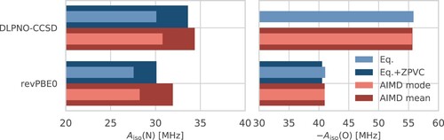
Table 6. ZPVCs and TFCs given for the HFCCs of nitrogen and oxygen in MHz at DLPNO-CCSD and revPBE0 level as depicted in Figure 6.

	$A_{\mathrm{iso}}$(N) (MHz)		$A_{\mathrm{iso}}$(O) (MHz)
	ZPVC	TFC	ZPVC	TFC
DLPNO-CCSD	3.5	4.3	–	0.2
revPBE0	2.5	4.4	0.5	0.3

Here, it is worth noting that the ZPVCs of VPT2 and the TFCs obtained from AIMD are, in principle, conceptually very different (Note that we also distinguish this strictly in our nomenclature by using the terms ZPVC and TFC). In VPT2, the expectation values for nuclear displacements and the corresponding corrections are purely quantum mechanical in nature, and it has been demonstrated for several properties that zero-point vibrational effects contribute the majority of the corrections [23,50,97]. In contrast to this, the AIMD simulates the classical motion of the freely rotating and vibrating molecule at 300 K. Hence, the TFCs obtained from averages over the trajectory can be considered a ”classical mechanics” correction. Furthermore, AIMD describes the ro-vibrational motion of HMI without separating its vibrations and rotations and also accounts for full anharmonicities and ro-vibrational couplings as described by classical statistical mechanics at 300 K on the full-dimensional global revPBE0-D3(0) potential energy surface (as generated on-the-fly).

Given the fundamentally different physics captured by the HFCC corrections provided by VPT2 and AIMD (evidently using the same DFT method), their above-mentioned similarity might appear puzzling at first glance. Yet, our finding that the quantum ZPVCs and the classical TFCs at 300 K are similar for HMI can be qualitatively explained as follows: HMI is a quasi-rigid molecule, as is the molecular core of most EPR spin probes, which implies that its heavy-atom cyclic skeleton undergoes only small-amplitude motion w.r.t. to its equilibrium geometry, both quantum-mechanically at 0 K and classically at 300 K. Being stiff, excited vibrational quantum levels of HMI are barely Boltzmann-populated at 300 K, meaning that the molecule essentially resides in its vibrational ground state at such temperatures. Next, small-amplitude vibrations are not expected to couple strongly to rotational motion and, for this reason, should not affect much the moment of inertia tensor of a rotating flexible but quasi-rigid molecule compared to its value at the equilibrium geometry. Last but not least, the harmonic oscillator approximation is fundamentally expected to work rather well for molecules which are subject to small-amplitude vibrational motion in the vibrational ground state. As a consequence, anharmonic corrections are small and second-order perturbation theory is very appropriate.

These general considerations now need to be connected to what is already known about temperature effects on top of ground state ZPVCs computed from VPT2 in the realm of magnetic properties of quasi-rigid molecules [50]. At 300 K, these TCs have been shown to be one order of magnitude smaller than the ZPVCs, meaning that corrections due to thermally populated excited vibrational states and changes of the moment of inertia tensor due to rotational motion are essentially negligible in view of the underlying relations as reported in Equations (4) and (5) of Ref. [50]. Given that we consistently use the same DFT methodology within VPT2 and AIMD, we conclude that VPT2 is a valid method to estimate the thermal average of HFCCs of quasi-rigid spin probe molecules, such as HMI, at ambient gas-phase conditions as provided by solving Equations 1(1) $\begin{array}{rl}⟨A⟩& =A_e+\sum _r{\left(\frac{\mathrm{\partial }A}{\mathrm{\partial }{Q}_r}\right)}_{Q_r=0}⟨Q_r⟩\\ & +\frac{1}{2}\sum _{r,s}{\left(\frac{{\mathrm{\partial }}^{2}A}{\mathrm{\partial }{Q}_r\mathrm{\partial }{Q}_s}\right)}_{Q_r,Q_s=0}⟨Q_r{Q}_s⟩\end{array}$(1) –3(3) $\begin{array}{rl}⟨Q_r{Q}_s⟩& ={\delta }_{\mathrm{rs}}\frac{\hslash }{4{\omega }_r}\end{array}$(3) for the molecular equilibrium geometry.

4.5. Computational cost

Considering that very similar results are obtained from the AIMD and the VPT2 calculations, it is worth comparing the computational time required for both approaches. The cost of a Born–Oppenheimer AIMD calculation is dominated by the SCF energy and gradient computed at every timestep. The simulation in the current work was performed on 8 nodes (each with 16 Intel Xeon E5-2630 v4 @ 2.20 GHz CPU cores) and took 571 h of wall clock time or about 73.000 core hours. On the other hand, the computational bottleneck in the VPT2 calculation is the 3N−11 Hessian calculations (175 for this system). At the revPBE0-D3(0) level of theory, these took about 2.5 h each, on 6 Intel Xeon E5-2687W v4 @ 3.00 GHz cores, or 2644 core hours in total, about 27 times less than the AIMD simulation.

When it comes to the single-point HFCC calculations, the revPBE0 ones took about 40 core minutes each, compared to 9500 core minutes (158 core hours) for DLPNO-CCSD. Considering the sample of 255 snapshot configurations, the additional single-point calculation cost is certainly negligible when using revPBE0, but adds up to 40.000 core hours when using DLPNO-CCSD. Note that the latter effort is already half of that invested into the hybrid AIMD simulations which were required to provide a statistically meaningful canonical sample of configuration snapshots of the quasi-rigid HMI molecule. While the computational effort is certainly not prohibitive, the analysis shows that the generation of sufficiently long trajectories and the large number of single-point calculations for snapshot calculations or property derivatives dominate the overall computational time. One should also point out that both, the AIMD and DLPNO-CCSD calculations exhibit an overall low scaling with system size, which should make similar simulations for larger systems feasible up to a certain point.

5. Conclusions

We have computed the HFCCs for the HMI molecule using DFT and DLPNO-CCSD, focusing on how modern local correlation methods can be used not only to provide equilibrium geometry properties but also vibrational and thermal corrections to the latter. For this purpose, we have tested two very different approaches: computing classical statistical-mechanical thermal averages at 300 K using AIMD simulations in the canonical ensemble in conjunction with single-point electronic structure-based property calculations versus directly computing quantum-mechanical ZPVCs using VPT2.

In agreement with previous studies, we found that correlation effects are essential for obtaining robust results for HFCC and that vibrational corrections can be sizeable. For a system of 31 atoms, DLPNO-CCSD calculations of HFCCs are perfectly feasible and a larger number of these can be carried out either in order to obtain vibrational corrections within VPT2 or to perform the thermal averages within AIMD based on many single-point property calculations.

In line with earlier findings by others when using the PBE0 hybrid density functional to compute EPR properties, we find that also the revPBE0-D3 functional, which is known to provide a very accurate full-dimensional global potential energy surface to describe liquid bulk water at 300 K, provides similar accuracy for open-shell molecules such as the HMI spin probe, albeit at an AIMD cost that is significantly increased compared to using the semilocal GGA cousin, namely revPBE-D3.

Convergence of the thermal property averages, based on a canonical sample of configurations to carry out the single-point electronic structure calculations in post-processing mode, is seen to set in at about 100 sufficiently uncorrelated snapshots in case of the small, stiff, and quasi-rigid HMI molecule in vacuum at 300 K.

For VPT2, 175 property calculations are required and overall the VPT2 route to vibrational corrections, also using revPBE0-D3(0), is less demanding computationally by one order of magnitude compared to hybrid AIMD. Comparing the canonical thermal averages of $A_{\mathrm{iso}}$, obtained from canonical AIMD simulations at 300 K, to the zero-point vibration-corrected equilibrium values of $A_{\mathrm{iso}}$ from VPT2, close agreement is observed for revPBE0-D3(0). This seems surprising at first sight since AIMD yields a finite-temperature classical-mechanical average that accounts for all ro-vibrational fluctuations, whereas VPT2 provides a zero-temperature quantum-mechanical average that considers vibrational motion in the quantum ground state. As explained in detail in the main part, this can be understood because HMI is a quasi-rigid molecule where the heavy-atom cyclic skeleton undergoes only small-amplitude motion w.r.t. to its equilibrium geometry, both classically at 300 K and quantum-mechanically at 0 K.

However, perturbative schemes typically require the computation of numerical derivatives, which limits the applicability of the DLPNO approximation in our case. Especially for small vibrational corrections, the numerical noise deteriorates the results for VPT2, while the averaging of snapshot results is much more robust as the procedure works in favour of filtering out statistical noise in the results.

Comparing DFT and DLPNO-CCSD vibrational corrections, we find that differences are much less pronounced than for the property itself, in agreement with previous studies on vibrational corrections of molecular properties. Given that a more sophisticated method is applied for the property calculation, the application of a more cost-effective electronic structure method for the vibrational corrections will be sufficient in many cases. Furthermore, VPT2 offers an efficient way to combine cost-effective methods for the evaluation of vibrational corrections as even very approximate methods like B97-3c seem to yield satisfactory anharmonic corrections and can at least be used to assess the magnitude of vibrational effects. These can in turn be used to estimate the thermal averages at 300 K for reasons just explained, thus connecting more directly to experimental data recorded at finite temperatures.

While there are no experimental reference values for the gas-phase HFCC of HMI, experimental studies on a nitroxide spin label belonging to the same heterocycle family as HMI by Smirnov et al. report the isotropic HFCC value for nitrogen to be about 40.0 MHz in an aprotic solvent like toluene [98]. Experiments have also shown that the isotropic HFCC increases for protic solvents and that explicit solvent interactions can have a large impact on the HFCCs [98–101]. An experimental study by Bobko et al. on the pH-sensitivity of nitroxide spin labels including HMI reports an isotropic nitrogen HFCC value in water of 44.8 MHz [102]. Considering the fact that no solvation effects were taken into account, the computed values in this work fall in a similar range, and the DLPNO-CCSD result (34.4 MHz) is closer to the experimental values than the revPBE0 one (31.9 MHz).

As an outlook, we therefore want to mention that AIMD simulations followed by DLPNO-CCSD property calculations allow one to not only compute thermal effects, but also solvent effects on EPR properties, such as $A_{\mathrm{iso}}$, at the identical level of accuracy as used in the present gas-phase study without resorting to common approximations such as microsolvation, continuum solvation, QM/MM, or MM solvation, which is essential for predictively bridging the theory-experiment gap in many cases. To this end, a very similar strategy can be followed, meaning the sampling of sufficiently many uncorrelated configuration snapshots of the solution, which faithfully represents the canonical ensemble of the spin probe in the liquid phase, thus including the thermal solvent fluctuations. In the subsequent step, single-point DLPNO-CCSD property calculations can be performed on this snapshot ensemble where, in stark contrast to the gas-phase case, a protocol for reducing the associated computational effort must be established and validated without sacrificing the desired DLPNO-CCSD accuracy. Such a controlled dimensional reduction step is necessary since – although non-periodic single-point DLPNO-CCSD property calculations are certainly feasible at the cutting-edge even when using about 100 water molecules as in periodic revPBE0-D3 AIMD simulations – the required DLPNO-CCSD calculations currently cannot be carried out routinely for many hundreds of such configuration snapshots. Joint research efforts in this direction are currently under way in our labs.

Acknowledgments

AAA would like to acknowledge Jürgen Gauss as mentor, supporter, and friend. FN thanks Jürgen Gauss for many years of support, friendship, and guidance. With his rigorous, careful, and unbiased approach to science, he has always been a role model and his work stands out as a great inspiration for thoroughness and the spirit of right-for-the-right-reason. We would like to acknowledge the Max-Planck Society and the IMPRS ‘Recharge’ for financial support. We would also like to acknowledge Marcus Kettner for initial work on the ORCA VPT2 module which has been extended to the computation of vibrational averages in this work. Funded by the Deutsche Forschungsgemeinschaft (DFG, German Research Foundation) under Germany's Excellence Strategy –EXC 2033 – 390677874 – RESOLV.

Disclosure statement

No potential conflict of interest was reported by the author(s).

Correction Statement

This article has been corrected with minor changes. These changes do not impact the academic content of the article.

Additional information

Funding

Funded by the Deutsche Forschungsgemeinschaft (DFG, German Research Foundation) under Germany's Excellence Strategy [grant number EXC 2033 – 390677874 – RESOLV] the Max Planck Society and the International Max Planck Research School on Reactive Structure Analysis for Chemical Reactions (IMPRS-RECHARGE).

References

- A. Schweiger and G. Jeschke, Principles of Pulse Electron Paramagnetic Resonance (Oxford University Press, New York, 2001).
- M. Kaupp, M. Bühl and V.G. Malkin, The Quantum Chemical Calculation of NMR and EPR Parameters. Theory and Applications (Wiley-VCH, Weinheim, Germany, 2004).
- F. Neese, Electron Paramagnetic Resonance (The Royal Society of Chemistry, Cambridge, 2007).
- F. Neese, Quantum Chemistry and EPR Parameters (American Cancer Society, Wiley, Chichester, 2017). pp. 1–22.
- J. Cížek and J. Paldus, J. Chem. Phys. 47, 3976 (1967).
- J. Cížek, J. Chem. Phys. 45, 4256 (1966).
- J. Cížek and J. Paldus, Int. J. Quantum Chem. 5, 359 (1971).
- J. Cížek, Adv. Chem. Phys. 14, 35 (1969).
- J. Paldus and J. Cížek, Chem. Phys. Lett. 3, 1 (1969).
- J. Paldus and J. Cížek, J. Chem. Phys. 52, 2919 (1970).
- K. Raghavachari, G.W. Trucks, J.A. Pople and M. Head-Gordon, Chem. Phys. Lett. 157, 479 (1989).
- S.A. Perera, J.D. Watts and R.J. Bartlett, J. Chem. Phys. 100, 1425 (1994).
- R. Improta and V. Barone, Chem. Rev. 104 (3), 1231–1254 (2004).
- S. Kossmann, B. Kirchner and F. Neese, Mol. Phys. 105 (15-16), 2049–2071 (2007).
- P. Verma, A. Perera and J.A. Morales, J. Chem. Phys. 139 (17), 174103 (2013).
- N. Rega, M. Cossi and V. Barone, J. Chem. Phys. 105 (24), 11060–11067 (1996).
- B. Fernndez, O. Christiansen, O. Bludsky, P. Jørgensen and K.V. Mikkelsen, J. Chem. Phys. 104 (2), 629–635 (1996).
- V. Barone and A. Polimeno, Phys. Chem. Chem. Phys. 8 (40), 4609–4629 (2006).
- J.R. Asher and M. Kaupp, ChemPhysChem 8 (1), 69–79 (2007).
- X. Chen, Z. Rinkevicius, Z. Cao, K. Ruud and H. Ågren, Phys. Chem. Chem. Phys. 13, 696–707 (2011).
- F. Egidi, J. Bloino, C. Cappelli, V. Barone and J. Tomasi, Mol. Phys. 111 (9–11), 1345–1354 (2013).
- X. Chen, Z. Rinkevicius, K. Ruud and H. Ågren, J. Chem. Phys.138 (5), 054310 (2013).
- A.Y. Adam, A. Yachmenev, S.N. Yurchenko and P. Jensen, J. Chem. Phys. 143 (24), 244306 (2015).
- F. Neese, F. Wennmohs and A. Hansen, J. Chem. Phys. 130 (11), 114108 (2009).
- F. Neese, A. Hansen and D.G. Liakos, J. Chem. Phys. 131 (6), 064103 (2009).
- C. Riplinger and F. Neese, J. Chem. Phys. 138 (3), (2013).
- C. Riplinger, P. Pinski, U. Becker, E.F. Valeev and F. Neese, J. Chem. Phys. 144 (2), 024109 (2016).
- Y. Guo, C. Riplinger, U. Becker, D.G. Liakos, Y. Minenkov, L. Cavallo and F. Neese, J. Chem. Phys.148 (1), 011101 (2018).
- P.R. Nagy, G. Samu and M. Kllay, J. Chem. Theory. Comput. 14 (8), 4193–4215 (2018). doi:10.1021/acs.jctc.8b00442.
- Q. Ma and H.J. Werner, J. Chem. Theory. Comput.14 (1), 198–215 (2018). doi:10.1021/acs.jctc.7b01141.
- C. Krause and H.J. Werner, J. Chem. Theory. Comput.15 (2), 987–1005 (2019). doi:10.1021/acs.jctc.8b01012.
- D.G. Liakos, Y. Guo and F. Neese, J. Phys. Chem. A 124 (1), 90–100 (2020).
- M. Saitow, U. Becker, C. Riplinger, E.F. Valeev and F. Neese, J. Chem. Phys. 146 (16), 164105 (2017).
- M. Saitow and F. Neese, J. Chem. Phys. 149 (3), 034104 (2018).
- D. Marx and J. Hutter, Ab Initio Molecular Dynamics: Basic Theory and Advanced Methods (Cambridge University Press, Cambridge, 2009).
- N.J. Russ and T.D. Crawford, J. Chem. Phys. 121 (2), 691–696 (2004).
- J.F.W. Keana, Chem. Rev. 78 (1), 37–64 (1978). doi:10.1021/cr60311a004.
- L.J. Berliner and J. Reuben, Spin Labeling Theory and Applications (Springer, US, 1989).
- N. Kocherginsky and H.M. Swartz, Nitroxide Spin Labels: Reactions in Biology and Chemistry (Taylor & Francis Inc, United States, 1995).
- V. Barone, Chem. Phys. Lett. 262 (3), 201–206 (1996).
- E. Bordignon, EPR Spectroscopy of Nitroxide Spin Probes (American Cancer Society, Wiley, Chichester, 2017). pp. 235–254.
- D. Marsh, Spin-Label Electron Paramagnetic Resonance Spectroscopy (Taylor & Francis, CRC Press, Boca Raton, Florida, 2019).
- V.V. Ptushenko, L.N. Ikryannikova, I.A. Grigor'ev, I.A. Kirilyuk, B.V. Trubitsin and A.N. Tikhonov, Appl. Magn. Reson. 30 (3), 329 (2006).
- A.N. Tikhonov, R.V. Agafonov, I.A. Grigor'ev, I.A. Kirilyuk, V.V. Ptushenko, and B.V. Trubitsin, Et Biophysica Acta, Biochim. Biophys. Acta. 1777 (3), 285–294 (2008).
- K. Ruud, P.O.A. strand and P.R. Taylor, J. Chem. Phys. 112, 2668 (2000).
- A.A. Auer, J. Gauss and J. Stanton, J. Chem. Phys. 118, 10407 (2003).
- I. Mills, J. Mol. Spectrosc. 5, 334–340 (1961).
- J. Geratt and I.M. Mills, J. Chem. Phys. 49, 1719 (1968).
- I.M. Mills, J. Phys. Chem. 80, 1187 (1976).
- M.E. Harding, M. Lenhart, A.A. Auer and J. Gauss, J. Chem. Phys. 128 (24), 244111 (2008).
- A.A. Auer, Chem. Phys. Lett. 467 (4), 230–232 (2009).
- J. VandeVondele and M. Sprik, Phys. Chem. Chem. Phys. 7, 1363–1367 (2005).
- F. Neese, Wiley Interdiscip. Rev. Comput. Mol. Sci. p. e1327 (2017).
- F. Weigend and R. Ahlrichs, Phys. Chem. Chem. Phys. 7 (18), 3297 (2005).
- F. Weigend, J. Comput. Chem. 29 (2), 167–175 (2008).
- C. Hättig, Phys. Chem. Chem. Phys. 7 (1), 59–66 (2005).
- Y. Zhang and W. Yang, Phys. Rev. Lett. 80, 890–890 (1998).
- S. Grimme, J. Antony, S. Ehrlich and H. Krieg, J. Chem. Phys. 132 (15), 154104 (2010).
- J.G. Brandenburg, C. Bannwarth, A. Hansen and S. Grimme, J. Chem. Phys. 148 (6), 064104 (2018).
- A.D. Becke, Phys. Rev. A 38 (6), 3098–3100 (1988).
- J.P. Perdew, Phys. Rev. B 33, 8822 (1986).
- S. Grimme, S. Ehrlich and L. Goerigk, J. Comput. Chem. 32 (7), 1456–1465 (2011).
- F. Weigend and M. Häser, Theor. Chem. Acc. 97 (1–4), 331–340 (1997).
- F. Weigend, M. Häser, H. Patzelt and R. Ahlrichs, Chem. Phys. Lett. 294 (1), 143–152 (1998).
- T.H. Dunning, J. Chem. Phys. 90 (2), 1007–1023 (1989).
- F. Weigend, Phys. Chem. Chem. Phys. 8 (9), 1057–65 (2006).
- F. Weigend, J. Chem. Phys. 116 (8), 3175–3183 (2002).
- D. Bykov, T. Petrenko, R. Izsák, S. Kossmann, U. Becker, E. Valeev and F. Neese, Mol. Phys.113, 1961–1977 (2015).
- J.P. Perdew, K. Burke and M. Ernzerhof, Phys. Rev. Lett. 77, 3865–3868 (1996).
- J.P. Perdew, K. Burke and M. Ernzerhof, Phys. Rev. Lett. 78, 1396–1396 (1997).
- A.D. Becke, Phys. Rev. A 38, 3098–3100 (1988).
- C. Lee, W. Yang and R.G. Parr, Phys. Rev. B 37, 785–789 (1988).
- V. Barone and P. Cimino, Chem. Phys. Lett. 454 (1–3), 139–143 (2008).
- T. Giovannini, P. Lafiosca, B. Chandramouli, V. Barone and C. Cappelli, J. Chem. Phys. 150 (12), 124102 (2019).
- O. Marsalek and T.E. Markland, J. Phys. Chem. Lett. 8 (7), 1545–1551 (2017).
- S. Imoto, H. Forbert and D. Marx, Phys. Chem. Chem. Phys. 17, 24224–24237 (2015).
- See https://www.cp2k.org.
- J. Hutter, M. Iannuzzi, F. Schiffmann and J. VandeVondele, WIREs Comput. Mol. Sci. 4 (1), 15–25 (2014).
- G. Lippert, J. Hutter and M. Parrinello, Mol. Phys. 92 (3), 477–488 (1997).
- J. VandeVondele, M. Krack, F. Mohamed, M. Parrinello, T. Chassaing and J. Hutter, Comput. Phys. Commun. 167 (2), 103–128 (2005).
- S. Goedecker, M. Teter and J. Hutter, Phys. Rev. B 54, 1703–1710 (1996).
- C. Hartwigsen, S. Goedecker and J. Hutter, Phys. Rev. B 58, 3641–3662 (1998).
- M. Krack, Theor. Chem. Acc. 114 (1), 145–152 (2005).
- L. Genovese, T. Deutsch, A. Neelov, S. Goedecker and G. Beylkin, J. Chem. Phys. 125 (7), 074105 (2006).
- L. Genovese, T. Deutsch and S. Goedecker, J. Chem. Phys. 127 (5), 054704 (2007).
- G.J. Martyna, M.L. Klein and M. Tuckerman, J. Chem. Phys. 97 (4), 2635–2643 (1992).
- F. Weigend, F. Furche and R. Ahlrichs, J. Chem. Phys. 119 (24), 12753–12762 (2003).
- D.E. Woon and T.H. Dunning Jr., J. Chem. Phys. 103 (11), 4572 (1995).
- R. Improta and V. Barone, Chem. Rev. 104 (3), 1231–1254 (2004). doi:10.1021/cr960085f.
- A.A. Auer, J. Gauss and M. Pecul, Chem. Phys. Lett. 368, 172 (2003).
- S.A. Katsyuba, E.E. Zvereva and S. Grimme, J. Phys. Chem. A 123 (17), 3802–3808 (2019).
- A.A.A. K.-H. Böhm and K. Banert, Molecules 19, 5301–5312 (2014).
- G. Rauhut, A.E. Azhary, F. Eckert, U. Schumann and H.J. Werner, Spectrochim. Acta Part A Mol. Biomol. Spectrosc. 55 (3), 647–658 (1999).
- G. Rauhut and H.J. Werner, Phys. Chem. Chem. Phys. 5 (10), 2001 (2003).
- T. Hrenar, H.J. Werner and G. Rauhut, J. Chem. Phys. 126 (13), 134108 (2007).
- A. Massolle, T. Dresselhaus, S. Eusterwiemann, C. Doerenkamp, H. Eckert, A. Studer and J. Neugebauer, Phys. Chem. Chem. Phys. 20, 7661–7675 (2018).
- D. Sundholm and J. Gauss, Mol. Phys. 92, 1007 (1997).
- A.I. Smirnov, A. Ruuge, V.A. Reznikov, M.A. Voinov and I.A. Grigor'ev, JACS 126, 8872–8873 (2004).
- T. Kawamura, S. Matsunami and T. Yonezawa, Bull. Chem. Soc. Jpn. 40, 1111–1115 (1967).
- A.V. Gagua, G.G. Malenkov and V.P. Timofeev, Chem. Phys. Lett. 56, 470–473 (1978).
- I. Al-bala'a and R.D. Bates, J. Magn. Reson. 73, 78–89 (1987).
- A.A. Bobko, I.A. Kirilyuk, N.P. Gritsan, D.N. Polovyanenko, I.A. Grigor'ev, V.V. Khramtsov and E.G. Bagryanskaya, App. Mag. Res. 39, 437 (2010).