
 ?Mathematical formulae have been encoded as MathML and are displayed in this HTML version using MathJax in order to improve their display. Uncheck the box to turn MathJax off. This feature requires Javascript. Click on a formula to zoom.
Abstract
Using the Weeks-Chandler-Andersen separation scheme, we explored equilibrium properties of fully penetrable soft spheres with an attractive tail. When the radial distribution function of the reference system is computed by means of the integral equation theory using the hyper-netted-chain closure, this separation scheme predicts pressure-density isotherms, vapour-liquid phase coexistence, and surface tension in good agreement with the results from Monte Carlo simulations even though the attractive portion of the interparticle potential has a significant effect on the radial distribution function. Despite its simplicity, the model potential we studied, with a certain parameter value, exhibits a non-monotonic temperature dependence of the liquid phase density over a wide range of pressure.
GRAPHICAL ABSTRACT
1. Introduction
Soft spheres are characterised by a repulsive pairwise interaction that increases relatively slowly with decreasing interparticle distance when compared to commonly used functions such as the Lennard-Jones potential. Soft spheres find their utility in studying colloidal suspension and polymer solutions [Citation1]. In recent years, soft spheres are often employed in meso scale simulations such as the dissipative particle dynamics (DPD) [Citation2].
These particles are often fully penetrable in that the interparticle potential remains finite even when multiple particles occupy exactly the same position in space. The simplest of such bounded interparticle potential models is a step function, for which the potential energy is a positive constant up to some cut-off interparticle distance and vanishes beyond this distance. Schmidt developed a density functional for this model fluid based on the fundamental measure theory and predicted bulk fluid properties accurately at low packing fractions [Citation3]. Other purely repulsive potentials, including Guassian core model [Citation4] and exponential core model [Citation5] were also studied.
The penetrable square well potential, a bounded version of square well potential, is the simplest model that exhibits vapour-liquid coexistence [Citation6–8]. To study interfacial phenomena by means of DPD, Liu et al. [Citation9] introduced a penetrable potential function constructed from cubic spline functions.
While particle based simulation techniques, such as molecular dynamics and Monte Carlo (MC) simulation [Citation10], remain the primary tools for exploring the physical properties and dynamical behaviour of soft spheres, the computational demands imposed by these methods justify an effort to explore the same using a more analytical and computationally less demanding approaches. It is also of great interest to explore how well the existing theories of liquids [Citation11] can predict the thermodynamic behaviour of soft spheres.
The integral equation theory is one such approach, in which one determines the radial distribution function by solving the Ornstein-Zernike (OZ) relation [Citation11]. Various equilibrium properties of the system follows from this function. Since the OZ relation involves the total and the direct correlation functions, both of which are unknown, it needs to be supplemented by an additional so-called closure relation involving these functions.
For soft spheres, the hyper-netted-chain (HNC) closure [Citation11] is known to yield a satisfactory result. The approach is particularly efficient computationally when applied to homogeneous phases. Recently, Malescio et al. [Citation12, Citation13] used HNC to successfully reproduce phase diagrams in qualitative agreement with simulation and to predict the onset of mechanical instability of high density liquid phases.
However, HNC is not without some serious limitations. If it is applied to a system capable of exhibiting the vapour-liquid phase coexistence, the solution often becomes increasingly difficult to find as one approaches unstable (or even metastable) states. While this may be reasonable on a physical ground, it frustrates an attempt to predict the phase diagram accurately. It also implies that physical properties of an inhomogeneous system cannot be studied by means of a simple gradient theory [Citation14–19], which requires the free energy density of a homogeneous system at all density values between those at the phase coexistence.
In this work, we consider three versions of HNC based approach. In the first version, which we shall refer to as HNC0, the full potential, consisting of both repulsive and attractive parts, will be treated by means of HNC. This version is subject to the limitations just indicated. In the second version, the potential energy is separated into a purely repulsive and a purely attractive parts according to the Weeks-Chandler-Andersen (WCA) scheme [Citation20]. Only the repulsive part is treated using HNC. When the contribution from the attractive part is treated by the first order perturbation theory, this leads to a scheme we refer to as WCA/P. By changing how we treat the attractive part, we arrive at the third version to be referred to as WCA/V. The predictions of these approaches will be compared against the results from MC simulations.
We introduce the model potential in Section 2 and describe our theoretical approach for computing thermodynamic properties in Section 3. Section 4 briefly describes the details of MC simulations. The results of our computations are presented in Section 5. We conclude the article with a few remarks in Section 6. Appendix provides a short derivation of the key formula for calculating the surface tension.
2. Model potential
Following the work of Ref. [Citation9], we consider the interparticle potential energy of the form
(1)
(1) where
(2)
(2) consists of cubic spline functions and has a continuous second derivative. In this work, we set
,
,
,
, and consider three values of
:
, 0.95, and 1. The resulting potential energy is shown in Figure .
Figure 1. Model potential given by Equations (Equation1(1)
(1) ) and (Equation2
(2)
(2) ).
,
,
, and
.
![Figure 1. Model potential given by Equations (Equation1(1) ϕ(r)=ε[Wcw(r/Rc)−Wdw(r/Rd)],(1) ) and (Equation2(2) w(x)={1−6x2+6x3(x≤1/2)2(1−x)3(1/2<x≤1)0(x>1).(2) ). ϵ=18.75, Wc=2, Rc=0.8, and Rd=1.](/cms/asset/fbccf6ae-66a3-4be8-a4de-651379c7f24c/tmph_a_1802076_f0001_oc.jpg)
Using the WCA separation scheme [Citation20], we split the potential energy at , where
takes its minimum value
, into the repulsive part:
(3)
(3) specifying the interparticle potential in the reference system, and the attractive part:
(4)
(4)
3. Integral equation theory
Let , where
is the inverse temperature, F is the Helmholtz free energy, and N is the number of particles in the system. Then,
(5)
(5) where Λ is the thermal wavelength of the particle and ρ is the number density of particles. The first two terms on the right-hand-side, taken together, represent the ideal gas contribution and
is the contribution to ψ arising from the interparticle potential.
Under the WCA separation of the potential energy, is further divided into
and
due, respectively, to
and
:
(6)
(6) For brevity and notational clarity, we present our method only for cases in which the WCA separation is employed (WCA/P and WCA/V). The formulation without this scheme (HNC0) can be recovered as a special case in which
and
. Accordingly
and
in HNC0.
3.1. Hyper-netted-chain closure
To determine , we find the radial distribution function
of the reference system by solving the OZ relation
(7)
(7) combined with the HNC closure:
(8)
(8) where
and
are direct and total correlation functions, respectively.
Once is found,
is obtained using a thermodynamic identity
(9)
(9) where
is the contribution to the pressure due to the repulsive interaction
and is evaluated by the virial equation of state as
(10)
(10) Under HNC [Citation11],
(11)
(11)
3.2. Perturbation theory
According to the first order perturbation theory,
(12)
(12) Once
is known, we can evaluate the contribution
to the pressure arising from
by
(13)
(13) Alternatively,
may be evaluated using the virial equation of state as
(14)
(14) Upon integration with respect to ρ, we obtain
(15)
(15) In the low density limit,
. Thus,
(16)
(16) This may be evaluated by a numerical quadrature and gives the value of the integrand in Equation (Equation15
(15)
(15) ) at
.
Equations (Equation12(12)
(12) ) and (Equation15
(15)
(15) ) define the methods we refer to as WCA/P and WCA/V, respectively. In both cases, the contribution from
to the chemical potential is given by
(17)
(17)
3.3. Phase coexistence
Densities of coexisting phases, and
, are determined by the equality of the pressures
(18)
(18) and that of the chemical potentials:
(19)
(19)
3.4. Inhomogeneous system
We resort to the gradient theory to describe a vapour-liquid interface. In this theory, the free energy of an inhomogeneous system is a functional of the density profile
and is given by [Citation14–19]
(20)
(20) where
is the free energy density of a bulk homogeneous phase and [Citation11, Citation18, Citation19]
(21)
(21) We used the random phase approximation to compute
:
(22)
(22) The surface tension γ of a vapour-liquid interface is given by [Citation19]
(23)
(23) where p and μ refer to the coexisting bulk phases. Appendix provides a short derivation of Equation (Equation23
(23)
(23) ).
3.5. Numerical procedure
Equations (Equation7(7)
(7) ) and (Equation8
(8)
(8) ) were solved iteratively to find
and
at evenly spaced 501 grid points on
. We examined the effect of doubling
or adding 500 more grid points under a few conditions. Except for a few instances to be stated explicitly, no discernible effect was observed.
At each temperature and density, HNC0 yields and
directly without requiring an integration with respect to ρ. Accordingly, we have considered only those density values around the phase coexistence. Since WCA/V requires integration with respect to ρ as indicated by Equation (Equation15
(15)
(15) ), we solved Equations (Equation7
(7)
(7) ) and (Equation8
(8)
(8) ) for well over 200 density values. WCA/P shares the same set of data with WCA/V.
This allowed us to find an initial estimate for the coexisting densities by plotting μ versus p curve using ρ as a parameter and finding the density values at which the curve intersects itself. The initial estimate was further refined using the Newton-Raphson method [Citation21].
In this and other computations, it becomes necessary to estimate various thermodynamic quantities and their density derivatives at arbitrary densities. For this purpose, we represented ,
,
, and
using a cubic spline interpolant. In constructing the interpolant, we used the fact that the first three of these quantities are zero at
. To evaluate
, we used the expression for
in the low density limit in Equation (Equation8
(8)
(8) ). Under the random phase approximation, this gives
(24)
(24) We also need to specify the density derivatives of the above listed quantities both at the lowest (
) and at the highest densities for which data is available. Following a recommendation in Ref. [Citation22], the derivative was estimated by representing the four data points at either end of the density values by a cubic polynomial.
A similar procedure was used for in WCA/P so that
can be evaluated by differentiation as indicated by Equation (Equation13
(13)
(13) ). In constructing the interpolant as described above, however, the following expression is available based on the low density approximation of
:
(25)
(25)
4. Monte Carlo simulation
To assess the accuracy of our theoretical methods, we performed a series of MC simulations in canonical and Gibbs ensembles [Citation23]. The bulk properties were computed not only for the system of particles interacting with the full potential φ, but also for the reference system in which the interparticle potential is purely repulsive and is given by Equation (Equation3(3)
(3) ).
The canonical ensemble simulation for bulk properties were performed in a cubic box of various sizes chosen to contain a reasonable number of particles. For ,
, and
, the side length of the cube was 20, 12, and 8, respectively. The surface tension was evaluated in canonical ensemble simulations involving 10000 particles in a rectangular box of height 40 and a square base with the side length 8. At each state point considered, we performed 10 independent simulations, each involving sampling over
MC cycles. The resulting error bars were smaller than the symbols used to represent the data, and will not be shown.
The Gibbs ensemble (GEMC) simulation involved two cubic boxes, one for the vapour phase and the other for the liquid. We adjusted the total number of particles so that the average volume for these boxes are approximately and
, respectively. Only one simulation, involving sampling over
MC cycles, was performed at each temperature value.
In all cases, the periodic boundary condition was applied in each direction and equilibration was carried out over at least MC cycles.
5. Results
To compare the HNC predictions, , for the radial distribution function against the results,
, of MC simulations, we quantified their difference by means of
(26)
(26) where we dropped the usual factor of
to emphasise the small r region (
), which is expected to have a more direct impact on the accuracy of the perturbation theory. Figure shows
for
and
. Since the unweighted average of
over the interval
is of the order of unity, we see that the error is generally well within a few % for both actual and reference systems. For the latter, there is a sudden increase in
at
. This is due to the finite size effect in MC simulations and results from our choice of the system volume described in Section 4. Using a larger system size reduced the magnitude of the jump, but only with a significant increase in the computational effort. For the actual system, the error is seen to grow rapidly towards the centre of the figure. This occurs as the system approaches the spinodal region (at
) or binodal lines (at
) either from the vapour or the liquid sides and the iterative solution of Equations (Equation7
(7)
(7) ) and (Equation8
(8)
(8) ) becomes increasingly difficult. The error
in this region, especially for the liquid phases, was slightly larger with
than with
(using
for both cases), presumably because correlations with longer wavelengths are permitted when
is larger.
Figure 2. Density dependence of the difference in the radial distribution functions between HNC and MC for the system interacting with the reference () and the full (φ) potentials.
.
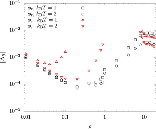
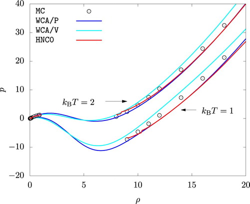
Figure shows the p versus ρ isotherms for the actual system. A good agreement is observed between the MC simulation on the one hand and predictions from HNC0, WCA/P, and WCA/V on the other. We note that MC results for the liquid phase fall between the predictions of WCA/P and WCA/V. Isotherms from HNC0 agrees more closely with WCA/P except for low density liquid phases. We also note that the HNC0 results show a discontinuous jump in pressure (at for
and at
for
). This occurs at higher densities if
. A convergent solution of Equations (Equation7
(7)
(7) ) and (Equation8
(8)
(8) ) became impossible to find at these densities if
. We took this as an indication that a homogeneous phase at these densities, at least according to HNC0, is unstable.
Figure 3. Pressure versus density isotherms. .
When computing by Equation (Equation10
(10)
(10) ), only the values of
in the range
are involved. In Figure , we compare
against
. While HNC is seen to be reasonably accurate in predicting
for both actual and reference systems, deviation from
is noticeable for
. In fact, when we set
in Equation (Equation26
(26)
(26) ),
of the actual system increased approximately by a factor of 2 for the vapour and 5 for the liquid phases. Nevertheless,
is still very small, and hence the good agreement we observed for p between MC and HNC0 is not surprising.
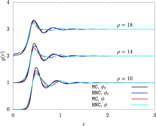
Figure 4. The radial distribution function from HNC and an MC simulation. To improve visibility, graphs for and 18 are shifted upwardly by 1 and 2, respectively.
and
.
A change in of a similar magnitude was observed for the reference system when we used
in Equation (Equation26
(26)
(26) ). In the case of WCA/P and WCA/V, however, the contribution from the attractive potential must also be included. Figure reveals a considerable difference in the radial distribution function between the actual and the reference systems. This situation is in stark difference from a system of Lennard-Jones particles, in which
of the reference system (defined by the WCA scheme) and the actual system are very similar, with nearly perfectly coincident r values for peaks and valleys of
.
To quantify the accuracy of the first order thermodynamic perturbation method, we evaluated the second order term using the approximate expression [Citation11, Citation24]:
(27)
(27) where
. In Figure , we compare
against
given by Equation (Equation12
(12)
(12) ). We observe that these two quantities are comparable at gas phase densities, but the importance of
decreases rapidly with increasing density. At
, for example,
is approximately 0.032 at
and 0.01 at
.
Figure 5. The relative importance in the thermodynamic perturbation theory of the second order term in comparison to the first order term
given by Equations (Equation27
(27)
(27) ) and (Equation12
(12)
(12) ), respectively.
.
![Figure 5. The relative importance in the thermodynamic perturbation theory of the second order term ψa(2) in comparison to the first order term ψa given by Equations (Equation27(27) ψa(2)(T,ρ)≈−14βρ(∂pref∂ρ)T−1∫[ϕa(r)]2gr(r)dr,(27) ) and (Equation12(12) ψa(T,ρ)=12βρ∫ϕa(r)gr(r)dr.(12) ), respectively. Wd=1.](/cms/asset/6a1dc170-35d8-4c55-8a31-583aff1b684d/tmph_a_1802076_f0005_oc.jpg)
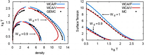
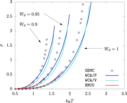
The phase diagrams from WCA/P and WCA/V are also in good agreement with the results from GEMC simulations as shown in Figures and . As with any other mean-field theory applied to model potentials with a harsh repulsive core, we observe that WCA/P and WCA/V both over-predict the critical temperature. For the range of values we considered, WCA/P and WCA/V predict very similar vapour phase densities, though the former tends to perform slightly better. In the case of the liquid phase, WCA/P is reasonably accurate for
and 0.95. For
, however, GEMC results tend to interpolate WCA/P and WCA/V over a wide range of temperature. HNC0 results are generally in agreement with WCA/P at low temperatures. For the liquid phase, they approach WCA/V results as temperature is increased. At higher temperatures, HNC0 failed to provide a convergent solution for ρ values around the phase coexistence. As a result, the binodal lines terminated prematurely as seen in Figure .
Figure 6. Phase diagram showing vapour-liquid phase coexistence.
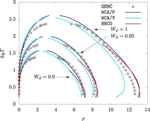
Figure 7. Vapor phase density at saturation.
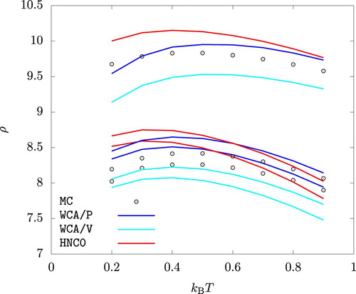
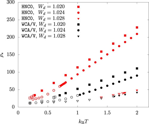
Interestingly, MC, HNC0, WCA/P, and WCA/V all predict that the liquid phase density for increases with increasing temperature up to
. This behaviour is related to the sign of the coefficient of thermal expansion,
, of the liquid phase at and near the phase coexistence. To see this, we note that
, and hence
(28)
(28) The Claussius-Clapeylon relation holds along the binodal lines:
(29)
(29) where
and
denote the entropy per particle in the liquid and the vapour phases, respectively. Eliminating dp from Equation (Equation28
(28)
(28) ), we arrive at
(30)
(30) where the subscript ‘vle’ indicates that the derivative is taken while maintaining the vapour-liquid phase coexistence. Insofar as the second term on the right hand side is expected to be positive,
if
. Figure shows that the latter derivative from MC simulations indeed is positive up to
over a very wide range of pressure. HNC0, WCA/P, and WCA/V all correctly capture this behaviour at least qualitatively.
Figure 8. Temperature dependence of the the liquid phase density at p = 0.01, p = 1, and p = 10. . For each method and at each temperature, the density is larger for a higher pressure.
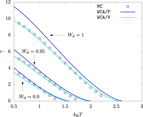
As shown in Figure , WCA/P and WCA/V both predict the surface tension γ reasonably well. WCA/V is more accurate at but WCA/P becomes comparably accurate as
is decreased. For all
values we studied, WCA/P and WCA/V over-predict γ at very high temperature values. This is a consequence of these theories over-predicting the critical temperature. We recall that HNC0 fails when applied to unstable phases and hence cannot be used to predict γ within the framework of the gradient theory.
Figure 9. Surface tension γ of the vapour-liquid interface at saturation.
For a sufficiently strong attractive potential, particles in the system may collapse to form a small blob. According to the Fisher and Ruelle criterion [Citation25, Citation26], the system at is unstable with respect to this collapse if
(31)
(31) which gives
for the model potential we are considering in this work. At non-zero temperatures, the entropic effect is expected to prevent the collapse if
is exactly 1.024. As
is increased, however, the collapse should be observable even at non-zero temperatures.
Taking the failure of the iterative solution of Equations (Equation7(7)
(7) ) and (Equation8
(8)
(8) ) as indicating the onset of this instability, Malescio et al. [Citation12, Citation13] showed that HNC0 predicts the onset in an excellent agreement with the Fisher and Ruelle criterion for several soft sphere potentials.
In contrast, we do not expect WCA/P or WCA/V to be capable of predicting this form of instability since the reference system for which HNC equation is solved is purely repulsive. Nevertheless, we found that WCA/V (as well as HNC0) predicts a form of mechanical instability (in addition to the spinodal) when the density is increased far beyond the liquid density at the vapour-liquid coexistence.
As an example, we considered three values:
, 1.024, and 1.028. The onset of this mechanical instability is identified by
(32)
(32) This equation is solved at various temperatures and the solution,
, is shown in Figure . At least for
and 1.024, WCA/V is seen to considerably underestimate
compared to HNC0. In both HNC0 and WCA/V, p decreased rapidly when ρ is increased beyond
. The iterative solution of Equations (Equation7
(7)
(7) ) and (Equation8
(8)
(8) ) eventually failed to converge at
.
Figure 10. The density , beyond which a high density fluid phase is mechanically unstable, plotted versus temperature. An open symbol indicates a fluid phase with a negative pressure.
In Figure , open symbols indicate that . Since the pressure takes the local minimum at the liquid phase spinodal density
before it reaches the local maximum at
, we have
. The vapour phase, if existed, should have a positive pressure. As a result, the system has no vapour-liquid coexistence at the temperature and the
value indicated by an open symbol in Figure . This means that, as the temperature is dicreased, the binodal lines terminate at T satisfying
, where
for a given
is a function of T only.
This is illustrated in Figure , which shows the liquid densities at saturation, , and
for
. Compared to HNC0, WCA/V predicts the termination of the binodal line (due to
being zero) at a much higher temperature. The HNC0 predictions follow the GEMC results more closely in this temperature range.
Figure 11. Liquid phase density at saturation () shown with the onset of mechanical instability (
) and the maximum density (
) above which iterative solution of Equations (Equation7
(7)
(7) ) and (Equation8
(8)
(8) ) fails.
. An open symbol for
indicates a negative pressure.
![Figure 11. Liquid phase density at saturation (ρleq) shown with the onset of mechanical instability (ρ⋆) and the maximum density (ρmax) above which iterative solution of Equations (Equation7(7) hr(r)=cr(r)+ρ∫cr(|r−r′|)hr(r′)dr′(7) ) and (Equation8(8) cr(r)=hr(r)−ln[hr(r)+1]−βϕr(r),(8) ) fails. Wd=1.024. An open symbol for ρ⋆ indicates a negative pressure.](/cms/asset/37230cbf-e1d3-4156-aba1-4bbef0bb54cd/tmph_a_1802076_f0011_oc.jpg)
However, the high density phase in GEMC simulation crystallised at and below , thus preventing a meaningful comparison between HNC0 and GEMC. The crystal phase had 4- and 6-fold rotational symmetries, pointing to the face-centred-cubic structure. As with
, WCA/V predictions of
are considerably smaller than those of HNC0. In agreement with what we saw for
, 0.95, and 1, the binodal line from HNC0 terminated prematurely as the temperature was increased.
WCA/P exhibited a rather peculiar behaviour at and 0.4. The p versus ρ isotherms have a local maximum at
, which is followed by a local minimum. With a further increase in ρ, p increased rapidly before the iterative procedure failed at the same
value as for WCA/V. (WCA/P and WCA/V share the same value for
, but not for
). The two extrema eventually merged into a single inflection point, which disappeared at around
. The sharp increase in p and the eventual failure of the iterative process were observed at all temperature values.
A failure of the iterative process is often identified as an onset of some instability. To gain an insight into the nature of this instability, we examined the radial distribution function and noticed an emergence and a sudden growth of a peak near r = 0. This is shown in Figure for using the value of
at r = 0.01, this value of r being the smallest available from our computation. Similar plots for other values of
(1.020 and 1.028) are omitted in the figures as they are indistinguishable from the graphs for
. The figure clearly indicates a significant overlapping of particles with increasing ρ as envisaged in the literature [Citation12, Citation13, Citation26].
Figure 12. Density dependence of the radial distribution function at r = 0.01 using the HNC closure. and
. The filled circules indicate the values at the onset of mechanical instability (
).
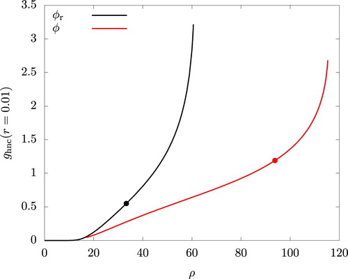
The rapid increase in occurs at lower densities for the reference system than for the actual system. This is expected and leads to the under-prediction of
and
by WCA/V mentioned earlier: The energetically favourable interaction is operational only for
, where
is determined by
, and this delays the overlapping of the particles in the actual system.
We emphasise that the overlapping of particles is observed even in the reference system, in which the interparticle potential is non-negative. There appears to be no reason for such particles to condense into a small blob. Even though a repulsive force from a single particle may be weak, a strong repulsive force would be generated if multiple of such particles fully overlap. Thus, it does not appear unreasonable to speculate that, at least in the case of the reference system and by extension in the actual system with small values, the new phase may be a crystal, in which each lattice point consists of multiple overlapping particles. A systematic exploration of this possibility would require a density functional theory of crystals [Citation27–29] along with extensive and very demanding (due to the very high density values involved) MC simulations, which is beyond the scope of this study.
6. Concluding remarks
We examined the accuracy of the WCA separation scheme for fully penetrable soft spheres with a bounded potential energy. When the total and direct correlation functions of the reference system are determined by the HNC closure, this separation scheme leads to predictions of equilibrium properties of both homogeneous and inhomogeneous systems in a good agreement with MC simulations. In contrast to more commonly studied potentials characterised by a harsh repulsive core, however, the radial distribution function of the reference system differs noticeably from that of the actual system.
The model potential we studied, despite its simplicity, leads to a non-trivial equilibrium behaviour. For example, the liquid phase density, as a function of temperature, is not monotonic over a very wide range of pressure at least for one of the values we examined. With increasing density, the liquid phase eventually becomes mechanically unstable. If the attractive part of the potential energy is sufficiently strong, we expect the liquid phase to collapse and form a high density blob. However, the reference system (without an attractive potential) is likely to form a crystal phase instead, in which each lattice point consists of multiple overlapping particles. Thus, unless the attractive potential is sufficiently strong, the above mentioned mechanical instability might point to a crystal phase formation. A systematic exploration of this possibility, however, is left to a future work.
Acknowledgments
Computations reported here were made possible by a resource grant from the Ohio Supercomputer Center [Citation30]. We are grateful for helpful comments from Professor Lisa M. Hall on the integral equation theory during the early stage of this work. A preliminary GEMC simulation carried out by Nicholas T. Liesen on soft spheres provided a motivation for this work.
Disclosure statement
No potential conflict of interest was reported by the author(s).
References
- P.G. Bolhuis, D. Frenkel, S.C. Mau and D.A. Huse, Nature 388, 235–236 (1997). doi:10.1038/40779
- P.J. Hoogerbrugge and J.M.V.A. Koelman, Europhys. Lett. 19, 155–160 (1992). doi:10.1209/0295-5075/19/3/001
- M. Schmidt, J. Phys. Condens. Matter 11, 10163–10169 (1999). doi:10.1088/0953-8984/11/50/309
- F.H. Stillinger, J. Chem. Phys. 65, 3968–3974 (1976). doi:10.1063/1.432891
- D.M. Heyes, Chem. Phys. 513, 174–181 (2018). doi:10.1016/j.chemphys.2018.07.037
- R. Fantoni, A. Giacometti, A. Malijevský and A. Santos, J. Chem. Phys. 133, 024101 (2010). doi:10.1063/1.3455330
- R. Fantoni, A. Malijevský, A. Santos and A. Giacometti, EPL 93, 26002 (2011). doi:10.1209/0295-5075/93/26002
- R. Fantoni, A. Malijevský, A. Santos and A. Giacometti, Mol. Phys. 109, 2723–2736 (2011). doi:10.1080/00268976.2011.597357
- M. Liu, P. Meakin and H. Huang, Phys. Fluids 18, 017101 (2006). doi:10.1063/1.2163366
- M.P. Allen and D.J. Tildesley, Computer Simulation of Liquids (Oxford University Press, New York, 1987).
- J.P. Hansen and I.R. McDonald, Theory of Simple Liquids: With Applications to Soft Matter, 4th ed. (Academic Press, Oxford, 2013).
- G. Malescio, Mol. Phys. 112, 1731–1735 (2014). doi:10.1080/00268976.2013.860246
- G. Malescio, A. Parola and S. Prestipino, J. Chem. Phys. 148, 084904 (2018). doi:10.1063/1.5017566
- J.D. van der Waals, J. Stat. Phys. 20, 200–244 (1979). doi:10.1007/BF01011514
- J.W. Cahn and J.E. Hilliard, J. Chem. Phys. 28, 258–267 (1958). doi:10.1063/1.1744102
- J.W. Cahn, J. Chem. Phys. 30, 1121–1124 (1959). doi:10.1063/1.1730145
- J.W. Cahn and J.E. Hilliard, J. Chem. Phys. 31, 688–699 (1959). doi:10.1063/1.1730447
- R. Evans, Adv. Phys. 28, 143–200 (1979). doi:10.1080/00018737900101365
- J.S. Rowlinson and B. Widom, Molecular Theory of Capillarity (Clarendon Press, Oxford, 1982).
- J.D. Weeks, D. Chandler and H.C. Andersen, J. Chem. Phys. 54, 5237–5247 (1971). doi:10.1063/1.1674820
- W.H. Press, S.A. Teukolsky, W.T. Vetterling and B.P. Flannery, Numerical Recipes (Cambridge University Press, Cambridge, 1992).
- D. Kahaner, C. Moler and S. Nash, Numerical Methods and Software (Prentice-Hall, Englewood Cliffs, NJ, 1989).
- A.Z. Panagiotopoulos, Mol. Phys. 61, 813–826 (1987). doi:10.1080/00268978700101491
- J.A. Barker and D. Henderson, J. Chem. Phys. 47, 2856–2861 (1967). doi:10.1063/1.1712308
- D. Ruelle, Helv. Phys. Acta 36, 183–197 (1963). doi:10.5169/seals-113366.
- D.M. Heyes and G.R. Rickayzen, J. Phys.: Condens. Matter 19, 416101 (2007). doi:10.1088/0953-8984/19/41/416101.
- W.A. Curtin and N.W. Ashcroft, Phys. Rev. A 32, 2909–2919 (1985). doi:10.1103/PhysRevA.32.2909
- W.A. Curtin and N.W. Ashcroft, Phys. Rev. Lett. 56, 2775–2778 (1986). doi:10.1103/PhysRevLett.56.2775
- A.R. Denton and N.W. Ashcroft, Phys. Rev. A 39, 4701–4708 (1989). doi:10.1103/PhysRevA.39.4701
- Ohio Supercomputer Center, Ohio Supercomputer Center (1987). <http://osc.edu/ark:/19495/f5s1ph73>.
- I. Kusaka, Statistical Mechanics for Engineers (Springer, New York, 2015).
- J.W. Gibbs, The Scientific Papers of J. Willard Gibbs, Vol. I. Thermodynamics (Ox Bow Press, Woodbridge, CT, 1993).
- K. Nishioka, Phys. Rev. A 36, 4845–4851 (1987). doi:10.1103/PhysRevA.36.4845
Appendix. Surface tension
The equilibrium density profile of a vapour-liquid interface (at the phase coexistence) is determined by minimising the grand potential , which is a functional of the density profile. Focusing on the unit area of the interface that runs perpendicular to the z-axis,
(A1)
(A1) where
and h is the height of the system with z = 0 at its centre. We place z = 0 within the interfacial region and suppose that h is taken sufficiently large so that
is well within the bulk phases.
As discussed in detail in Ref. [Citation19], we can profitably exploit the analogy with mechanics by regarding z as the time and ρ as the position of a particle subject to the potential energy . The mass of the particle is position dependent and is given by
.
In this mechanical analogy, Equation (EquationA1(A1)
(A1) ) is the action integral in which
(A2)
(A2) is the Lagrangian. Lagrange's equation of motion
(A3)
(A3) leads to
(A4)
(A4) where
and
(A5)
(A5) The non-linear second order ordinary differential equation, Equation (EquationA4
(A4)
(A4) ), would have to be solved numerically under the boundary conditions that
and
. This proves to be a rather non-trivial task due to (1) the existence of the additional solutions
and
besides the one we seek, (2) an extreme sensitivity of the numerical solution to the initial value of
, say at z = 0 where we may set
, and (3) the failure of the most of the differential equation solvers to conserve a constant of motion exactly even in a simpler case in which
is independent of ρ.
Fortunately, the mechanical analogy mentioned above reveals the existence of the first integral of Equation (EquationA4(A4)
(A4) ). In fact, since L does not depend explicitly on z, the energy function
(A6)
(A6) is a constant of motion [Citation31], and hence is independent of z. Evaluating the right-hand-side of Equation (EquationA6
(A6)
(A6) ) for either of the bulk phases at coexistence, in which
, we find that
. Recalling the double-tangent construction, by means of which one can find the coexisting densities [Citation31], we see that
. Thus, solving Equation (EquationA6
(A6)
(A6) ) for
and arbitrarily choosing the negative root so that the liquid phase is on the left of the vapour phase, we arrive at [Citation19]
(A7)
(A7) It is relatively easy to solve this first order ordinary differential equation numerically using, for example, the fourth order Runge-Kutta method under the boundary condition that
at z = 0 and integrating in both positive (vapour phase) and negative (liquid phase) directions.
The surface tension is the excess per unit area of the interface of the grand potential over that of the hypothetical system [Citation31–33]. The latter consists of bulk vapour and liquid phases in contact with each other across a sharp dividing surface parallel to the interface, but each behaving as if it is a piece of a bulk homogeneous phase. This leads to the following expression for γ:
(A8)
(A8) Using Equation (EquationA6
(A6)
(A6) ), we can rewrite this equation as
(A9)
(A9) Another application of Equation (EquationA7
(A7)
(A7) ) results in Equation (Equation23
(23)
(23) ). Clearly, it is unnecessary to find
if we are interested in γ only.