
 ?Mathematical formulae have been encoded as MathML and are displayed in this HTML version using MathJax in order to improve their display. Uncheck the box to turn MathJax off. This feature requires Javascript. Click on a formula to zoom.
Abstract
A wide class of coupled-cluster methods is introduced, based on Arponen's extended coupled-cluster theory. This class of methods is formulated in terms of a coordinate transformation of the cluster operators. The mathematical framework for the error analysis of coupled-cluster methods based on Arponen's bivariational principle is presented, in which the concept of local strong monotonicity of the flipped gradient of the energy is central. A general mathematical result is presented, describing sufficient conditions for coordinate transformations to preserve the local strong monotonicity. The result is applied to the presented class of methods, which include the standard and quadratic coupled-cluster methods, and also Arponen's canonical version of extended coupled-cluster theory. Some numerical experiments are presented, and the use of canonical coordinates for diagnostics is discussed.
GRAPHICAL ABSTRACT
1. Introduction
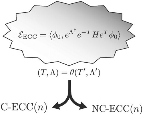
It is with delight that the authors dedicate this work to Professor Jürgen Gauß on the occasion of his sixtieth birthday. In the spirit of his pursuit of scientific rigour, especially the attention to detail in coupled-cluster (CC) theory, we here present a mathematical study of some alternative formulations based on Arponen's extended CC (ECC) method [Citation1,Citation2]. The ECC method is defined in terms of the critical points of an energy functional,
(1)
(1) where T and Λ are cluster operators in the usual sense of CC theory. The well-known CC Lagrangian introduced by Helgaker and Jørgensen [Citation3] is obtained by expanding
to first order. In this sense, the standard CC approach is an approximation to the ECC method.
We will study a collection of methods that generalises this idea, defined by substitution of by a Taylor polynomial of fixed degree n. This can be formulated as a coordinate transformation of the cluster amplitudes. A second class of models is obtained by a further coordinate transformation introduced by Arponen to ensure a certain linkedness structure of the energy functional. We refer to these coordinates as canonical, as the time-dependent Schrödinger equation takes the form of Hamilton's equations of motion in this case. Thus, we obtain two hierarchies NC-ECC
, using non-canonical coordinates, and C-ECC
using canonical coordinates. Our mathematical results imply that when the cluster operators are not truncated, all these models are exact and equivalent to the time-independent Schrödinger equation. Moreover, Galerkin approximations (i.e. generic truncation schemes that can approach the untruncated limit) will converge under certain relatively mild single-reference-type conditions. While the methods discussed here are all expensive (for n>1), we consider them as stepping stones towards producing competitive alternatives to standard CC theory that alleviate deficiencies of the latter, such as the inability to correctly break chemical bonds.
The various forms of CC methods are today among the most widely used for wavefunction-based calculations on manybody systems. The main idea stems from Hubbard's exponential parameterisation of the wavefunction based on cluster operators in manybody perturbation theory [Citation4], which was taken as starting point for ab initio treatments by Coester and Kümmel for nuclear structure calculations in the 1950s [Citation5,Citation6]. The modern form of standard CC theory was developed by, among others, Sinanoğlu, Paldus and Cizek in the 1960s [Citation7] and the CC method with singles, doubles and perturbative triples [CCSD(T)] today constitutes ‘the gold standard of quantum chemistry’ due to its excellent balance between computational cost and accuracy [Citation8]. In nuclear structure calculations the same method has gained traction in the last decade, providing excellent predictive power for light to medium nuclei [Citation9]. Coupled-cluster theory has also been applied to superconductivity [Citation10], lattice gauge theory [Citation11], and systems of trapped bosons such as Bose–Einstein condensates [Citation12]. These examples and the cited works are by no means exhaustive, but serve to illustrate the flexibility of the CC formalism.
In the early 1980s, Arponen introduced a novel concept into CC theory, namely the bivariational principle [Citation1,Citation13], resulting in the ECC method [Citation1,Citation2,Citation14], and an interpretation of standard CC theory and ECC theory as variational methods in a more general sense, i.e. they are bivariational. However, the ECC method has seen little use in chemistry due to its immense complexity, even for truncated versions. In physics, on the other hand, the ECC model has advantages over standard CC theory that can make it very useful. To illustrate, the ECC method correctly describes symmetry breaking in the Lipkin–Meshkov–Glick quasispin model of collective monopole vibrations in nuclei [Citation13,Citation15], in contrast to the standard CC method, which cannot. For the electronic-structure problem in quantum chemistry, the standard CC model fails dramatically to reproduce dissociation curves of even simple dimers like , while the ECC method performs quite well [Citation16,Citation17]. Thus, we are of the opinion that the ECC method is still worthwhile to study, and approximate forms may still prove to be useful in quantum chemistry.
The non-canonical and canonical hierarchies (N)C-ECC(n) introduced in this article turn out to be equivalent, and give identical predictions, when truncated with an excitation-rank complete scheme. On the other hand, the working equations are different and in fact cheaper in the canonical case, albeit marginally. An example is the NC-ECC(1)SD method, i.e. the standard CCSD approach, and the C-ECC(1)SD method, which are equivalent. We also raise the question about diagnostics for practical calculations, and show some numerical evidence that diagnostics can favourably be done using canonical coordinates, even if the computations are done in the usual manner using non-canonical variables.
Another well-known special case is NC-ECC(2), the quadratic coupled-cluster (QCC) method introduced by Van Vorhiis and Head-Gordon [Citation18,Citation19], whose canonical and non-canonical versions are equivalent in their doubles-only approximation. We note that the asymptotic cost of QCCD is the same as CCSD, even if it is a higher-order approximation to ECC. Furthermore, the perfect-pairing (PP) hierarchy [Citation20] of amplitude truncation schemes can be applied to our methods. The PP hierarchy are approximations to the complete-active space self-consistent field (CASSCF) method, including only a tiny subset of even-rank amplitudes combined with orbital optimisation, the latter which we disregard here. The corresponding canonical and non-canonical formulations (N)C-ECC(1)PPH are inequivalent. The n>1 versions could also be interesting in their own right, as investigated by Byrd and coworkers in the case of the QCC method [Citation19].
The remainder of the article is organised as follows: In Section 2, we introduce the bivariational principle and the mathematical setting of local analysis of CC methods. The key concept of our analysis is the notion of local strong monotonicity of the flipped gradient of a smooth bivariational energy functional (see Equation (Equation7(7)
(7) )). The usefulness of this property is presented in Theorem 2.1, where local uniqueness and quadratic error estimates are established in a very general setting using Zarantonello's Theorem from nonlinear monotone operator theory [Citation21,Citation22]. Next, Theorem 2.2 summarises the main results of Ref. [Citation23], where strong monotonicity is proven for the non-canonical ECC method. For a recent review on monotonicity in CC theory we refer to [Citation24], where this property is linked to spectral gaps of the systems under study. Section 3 presents the idea of monotonicity-preserving coordinate transformations. Our main result, Theorem 3.1, is a change-of-coordinates result. When combined with Theorems 2.1 and 2.2, the analysis of (N)C-ECC(n) follows in Corollary 3.2. Our tools rely heavily on the functional analytic formulation of cluster operators and the Schrödinger equation developed by Rohwedder and Schneider [Citation25–27]. The results are formulated in a qualitative manner, in the sense that they are indeed rigorous but depend on constants whose numerical (or optimal) values are unknown. We leave further quantitative investigations for future work. In Section 4, we perform some numerical experiments to elucidate some aspects of the (N)C-ECC(n) hierarchies, before we finish with some concluding remarks in Section 5. All the proofs of our results are presented in Appendix.
2. The non-canonical extended coupled-cluster model
2.1. Bivariational principle
The starting point is a generalisation of the Rayleigh–Ritz variational principle to operators that are not necessarily self-adjoint (Hermitian in the finite-dimensional case). For simplicity, we assume a real Hilbert space . Given a system Hamiltonian
, where
is dense, we define a bivariate Rayleigh quotient,
,
(2)
(2) Requiring the functional
to be stationary at
with respect to arbitrary variations in the two wavefunctions leads to the conditions
,
and
, with
, i.e. the right and left eigenvalue problem for
. If
is self-adjoint, the eigenfunctions are identical up to normalisation. The introduction of two independent wavefunctions therefore might seem to complicate matters. However, the bivariate Rayleigh quotient
allows distinct approximations of ψ and
, introducing more flexibility for approximate schemes. Moreover, the state defined is a (non-Hermitian) density operator, which is unique,
When determined variationally, the Hellmann–Feynman theorem [Citation28] gives well-defined physical predictions in terms of ρ.
As is common in analysis of partial differential equations [Citation29,Citation30], we pass to a weak formulation, which in this case is equivalent to the strong formulation outlined above. Under the assumption that is below bounded, we can introduce a unique extension
(dual space), where
is a dense subspace, a Hilbert space with norm
, continuously embedded in
. It follows that
is continuously embedded in
, and we have a scale of spaces with dense embeddings,
. The operator H is bounded (i.e. continuous), and satisfies a Gårding estimate, i.e. for some
and some
,
for all
. For the electronic-structure problem
can be taken to be the space of square-integrable functions with finite kinetic energy.
If is finite-dimensional, we can set
, simplifying matters a lot, and the reader may if she or he wishes stick to this picture for simplicity, where all operators are basically matrices. In the infinite-dimensional case, however,
is typically unbounded as an operator over
, and the above construction is necessary.
Under the stated conditions, is a (Fréchet) smooth map away from the singularity
, and Taylor series exist and converge locally, allowing a certain degree of intuition to be borrowed from the finite-dimensional case. The right and left Schrödinger equations are then
and
, respectively. This is the bivariational principle.
2.2. Exponential ansatz and the ECC method
The standard CC method is formulated relative to a fixed reference on determinantal form. By introducing a cluster operator
with
containing all excitations of rank k, i.e. of k fermions relative to
, we have the exact parameterisation
assuming intermediate normalisation,
.
Since all excitations commute, the cluster operators form a commutative Banach algebra under suitable conditions which we now describe [Citation25,Citation26]. We expand the cluster operators using amplitudes and basis operators, i.e. , where
excites a number
of fermions in the reference into the virtual space, i.e.
where the
are among the occupied orbitals of
, and
among the unoccupied orbitals. The set
is the generic set of amplitude indices. We introduce a Hilbert space
with norm
, which becomes a useful space for formulating abstract CC theory. Fundamental results include that any
is a bounded operator on
, such that, e.g.
also is a bounded operator. Moreover,
is also a bounded operator, which means that we can make sense of, e.g.
, and that we can represent any intermediately normalised
as
with
unique. Finally, all the elements of the algebra are nilpotent. The Banach algebra structure on
allows CC theory to be rigorously formulated in the full, infinite-dimensional case. This was the approach taken in Ref. [Citation23] for a first analysis of NC-ECC theory.
Again, the finite-dimensional case may by kept in mind: In this case, cluster amplitudes are simply finite-dimensional vectors, and the existence of the exponential parameterisation is a trivial result. There is no need to introduce the norm , instead the Euclidean norm on the amplitudes may be used.
Any normalised according to
can be represented by introducing a second cluster operator
, viz.,
Inserting the parametrization of ψ and
into the bivariate Rayleigh quotient, we obtain the energy functional
of the non-canonical ECC method, given in Equation (Equation1
(1)
(1) ). This map is everywhere smooth, and its critical points
are equivalent to the Schrödinger equation and its dual: Under the assumption that the eigenfunctions can be normalised according to
,
and
solve the Schrödinger equation and its dual if and only if
(3)
(3) Assuming that the eigenvalue
is non-degenerate,
is easily seen to be locally unique.
2.3. Truncations and monotonicity analysis
The non-canonical ECC energy is just one out of many possible parameterisations of the exact bivariate Rayleigh quotient . In this section, we take a more abstract approach and consider a general energy functional
, obtained by some exact parameterisation of
by means of the space
, i.e. by a pair of cluster operators
. We will discuss several such functionals in Section 3, obtained from the NC-ECC functional by coordinate transformations.
Only in rare cases can the amplitude equations (Equation3(3)
(3) ) be solved exactly. Introduce therefore a discretised space
of finite dimension by truncating the amplitude index set
, that is,
if and only if
(4)
(4) The set
is typically defined by the restriction of the excitations to a finite virtual space (a finite basis), and to a finite excitation rank (smaller than the number of electrons). In the chemistry literature, the excitation hierarchy for a given basis is traditionally denoted singles (S), doubles (D), and so on. In the ECC literature, one typically speaks of the SUBn approximation, with n being the maximum rank.
When the discrete space is established, we define a discrete solution by the stationary conditions of the restricted energy function . The stationary equations take the form
(5)
(5) for all
.
It is not necessary to use the traditional truncation scheme outlined here; any increasing sequence of subspaces , with d a parameter, that can approximate elements in
arbitrarily well by increasing d can be used. We let
be the distance from v to
measured with respect to the norm of
. Consequently, for all
we have
as
. Such a sequence of spaces is referred to as a Galerkin sequence. Other options than the traditional truncation schemes are explicitly correlated methods [Citation31] and complete-active space methods [Citation20,Citation32,Citation33] such as the PP hierarchy.
An often overlooked point in the physics literature is the fact that convergence of the equations does not in general imply convergence of their solutions. An important question is therefore whether the discrete critical points converge to the exact critical points
as
. This would imply that the energy converges too, and in a quadratic manner due to the critical point formulation.
Monotonicity is an important notion in connection with the local analysis of the CC method and its variations [Citation23–27,Citation34]. The use of monotonicity in the analysis of the standard CC method was introduced by Schneider and Rohwedder [Citation25,Citation27]. The intuition behind (strict) monotonicity is that of an everywhere (strictly) increasing (or decreasing) function. The function that one studies is typically a root problem such as the CC amplitude equations , where
. Monotonicity allows the establishment of locally unique solutions of the Galerkin problem and is therefore important for the motivation of numerical implementations. As such it is a fundamental result of the CC method's practical usage in quantum chemistry. It also connects spectral gaps, e.g. HOMO-LUMO gap, to stability constants within the analysis [Citation24]. (See also the steerable CAS-ext gap connected to the tailored CC method [Citation35] that treats quasi-degenerate systems [Citation36].)
The particular monotonicity property that is key for this presentation is an even stronger version than that of strict monotonicity, and is called strong monotonicity. It is defined as follows: A finite-dimensional vector-valued function is locally strongly monotone near some
if for
in a neighbourhood of
we have
(6)
(6) for some constant
. (In the infinite-dimensional case
is the dual pairing, which then becomes an infinite sum, see Ref. [Citation23] for more details.)
Furthermore, we need the concept of Lipschitz continuity: F is locally Lipschitz continuous with constant L>0 if
In particular, any (Fréchet) smooth function is locally Lipschitz continuous, and so are all its derivatives.
The map F that we will study is the flipped gradient of the general energy functional , defined as
(7)
(7) or more compactly
, with R being the map that exchanges the partial derivatives. The motivation is as follows: If we consider the bivariate Rayleigh quotient,
is not locally strongly monotone, as its critical points are saddle points. On the other hand, the flipped gradient
can be seen to be locally strongly monotone near the ground state, given that this ground state is non-degenerate with a nonzero spectral gap to the remaining spectrum. It is natural to expect that one can find conditions such that the flipped gradient of the energy when expressed in new coordinates is locally strongly monotone.
The following is a central result, adapting a result due to Zarantonello [Citation21,Citation22] (points 1 and 2) to the present notation and setting, and applied to the flipped gradient of an energy functional (point 3).
Theorem 2.1
General convergence and error estimates
Let be a map, and let
be an open ball containing a
such that
.
Let be a Galerkin sequence of subspaces with
being the orthogonal projector onto
. Furthermore, let
be the Galerkin discretisation of F, i.e.
.
Assume that F is locally strongly monotone with constant and Lipschitz continuous with constant L>0 on U. Then, the following holds:
| (1) |
| ||||
| (2) | There is a sufficiently large | ||||
Let ,
be a (Fréchet) smooth energy functional. Let R be the flipping map as introduced after Equation (Equation7
(7)
(7) ) and set
, and
.
| (3) | For | ||||
The proof is presented in Appendix. The error estimate (Equation9(9)
(9) ) shows that for (smooth) energy functionals with a locally strongly monotone flipped gradient, the bivariational method of discretisation behaves very similar to the usual Rayleigh–Ritz variational method of discretisation. As we enlarge the Galerkin space, the discrete ground state converges, and the energy error is quadratic in the error of the state. However, we cannot guarantee convergence from above, but this is much less important than actually having a quadratic error.
An interesting fact is that Brouwer's fixed point theorem [Citation37] can be used to obtain a sufficient condition for the constant , where quadratic convergence sets in, namely
(10)
(10) see Refs. [Citation23,Citation26]. The radius δ of the domain U in Theorem 2.1 is unknown in general, and we see that a small monotonicity constant η relative to L will be severely detrimental for the convergence, as it forces
to be very large. On the other hand, in general one has that η and the Lipschitz constant L are related by
. The optimal value of the right-hand side is therefore
.
The following theorem summarises the main results of Ref. [Citation23], where the proof and more details can be found:
Theorem 2.2
NC-ECC monotonicity
Assume that the system Hamiltonian is self-adjoint, and that the ground state of
exists, is non-degenerate, and that there is a spectral gap
between the ground-state energy
and the rest of the spectrum. Assume that the reference
is such that it is not orthogonal to the ground-state wavefunction. Let
be the corresponding critical point of
, and assume that
and
are not too large, i.e. that
is a sufficiently good approximation to
. Then,
is locally strongly monotone near
with a constant
, for some C<1.
The consequence of Theorem 2.2, when combined with Theorem 2.1, is that the non-canonical ECC method is convergent as the discrete cluster amplitude space approaches the untruncated limit. As already remarked, we do not explicitly know the onset
of quadratic convergence.
3. Monotonicity-preserving coordinate transformations
3.1. A class of exact coupled-cluster models
In addition to the non-canonical ECC parameterisation, Arponen also considered a second parameterisation of the bra and ket wavefunctions, which gives equations of motion for the time-dependent Schrödinger equation that are canonical in the sense of Hamiltonian mechanics [Citation1,Citation2]. (This must not be confused with the use of canonical Hartree–Fock orbitals, which is unrelated.) This parameterisation is given in terms of a coordinate transformation as
(11)
(11) where
, and
is defined by
(12)
(12) This function has inverse
. (In Arponen's work [Citation2], the notation
is used.) The map
is smooth and invertible with a smooth inverse, and we therefore obtain a new exact energy functional
with values
(13)
(13) A remarkable consequence of this second parameterisation is that it corresponds to retaining only those terms in Equation (Equation1
(1)
(1) ) that can be represented by ‘doubly linked’ diagrams [Citation1,Citation2],
(14)
(14) The phrase ‘doubly linked’ means that every power of
is connected to two
operators on its right, unless it is connected directly to H. The subscript ‘C’ for ‘connected’ is the usual connectedness criterion on contractions between H and powers of
[Citation8]. Thus, the canonical coordinates represent a more compact representation in that the resulting tensor contractions or diagrams in the energy are identical to those obtained in the NC-ECC energy (Equation1
(1)
(1) ), except for some diagrams that are explicitly eliminated.
Similarly, for the standard CC method, Arponen introduced the coordinate transformation given by
(15)
(15) We obtain the energy functional
, where
(16)
(16) that is, the standard CC Lagrangian [Citation3]. Incidentally, the standard CC coordinates are also canonical.
The map can be generalised to Taylor polynomials. By setting
we can solve for Λ in terms of
by, e.g. considering first the singles, then doubles, etc., giving a smooth map
such that
. In fact, since the cluster operators are nilpotent,
, where the logarithm is expanded in a (finite) Taylor series around the identity. Similarly, we can solve for
in terms of Λ, demonstrating that this map has an inverse, and in fact that this inverse is smooth. We obtain a coordinate transformation
given by
(17)
(17) and the corresponding energy functional
(18a)
(18a) Coordinate transformations form a group, and may thus be composed. By combining
, we obtain an energy functional
(18b)
(18b) Since, in the NC-ECC energy functional (Equation1
(1)
(1) ), an exponential
can be inserted after
without changing the result, both of these hierarchies correspond to truncations of a Baker–Campbell–Hausdorff expansion at order n, and are thus manifestly extensive.
3.2. Coordinate transformation theorem
Equations (Equation18a(18a)
(18a) ) and (Equation18b
(18b)
(18b) ) represent two hierarchies of exact parameterisations of the bivariate Rayleigh quotient. It is therefore of interest to determine whether they have locally strongly monotone flipped gradients. To establish this, we study the effect on local strong monotonicty of a coordinate transformation.
Theorem 3.1
Coordinate transformations
Let be a smooth energy functional, let
be a critical point, and assume that
is locally strongly monotone near
with constant
. Let a smooth
with a smooth inverse be a given coordinate transformation, and let
be the energy functional expressed in the new coordinates. Let
be the corresponding critical point for
, and let
be its flipped gradient. Let
be the Jacobian at
. Then we have the following conclusions:
| (1) | If | ||||
| (2) | In the noncommuting case, if | ||||
Theorem 3.1 tells us that if we create a new method by changing coordinates in a sufficiently well-behaved manner, the monotonicity of the flipped gradient of the energy will be preserved. Hence, the new method will be convergent in the sense of Theorem 2.1, if the original method is. This gives us great flexibility in choosing new cluster-operator parameterisations, since we already know that non-canonical ECC is convergent. The interested reader can find the proof in the Appendix.
3.3. Monotonicity of (N)C-ECC models
We apply Theorem 3.1 to the maps and
that define the NC-ECC
and C-ECC
models, respectively. The conclusion is as follows (with proof given in the Appendix):
Corollary 3.2
For any of the NC-ECC or C-ECC
models, the assumption that the ground-state critical point
is not too large together with a spectral gap
is sufficient to guarantee local strong monotonicity of the flipped gradient of the energy, and hence a quasi-optimal solution to the Galerkin problem and a quadratic error estimate for the energy.
We note that our estimates are probably pessimistic for some of the models covered here. The analysis starts with a given monotonicity constant η for the NC-ECC scheme, depending on the spectral gap, and consistently produces an for the method obtained using the coordinate change, worsening the error estimates. It may well be that a direct analysis of the secondary method yields a better
. The assumptions on the Hamiltonian and reference may also become milder. However, the important point here is that Theorem 3.1 does guarantee that the new method is convergent under some reasonable conditions. For example, we have now proven that QCC theory [Citation18] is convergent if the reference is a sufficiently good approximation to the ground state, and using Equation (Equation10
(10)
(10) ) also a basic means to study which truncations or Galerkin schemes can be reasonable, at least in principle. It may be interesting to see whether truncation schemes like the PP hierarchy with orbital optimisation, also in a quadratic n = 2 or higher formulation [Citation19], can be further analysed based on our results.
In the proof of Theorem 3.1 (see Appendix), it arises naturally that the most favourable coordinate transformations are those that commute with the flipping map R, since local strong monotonicity then follows with no assumptions on the Jacobian of the map. The Jacobian commutes with R if and only if
(19)
(19) and one must assume that this holds at every point in
, as one does not know a priori where the critical point is. It is not clear what such transformations in general look like, and whether such transformations are useful reparameterisations of the energy.
3.4. Properties of the canonical and non-canonical schemes
The coordinate transformation as represented by Equation (EquationA7
(A7)
(A7) ) is such that when applied to a cluster operator
of rank k, it generates terms
with
. The same is true for the inverse map. Thus, if
is excitation-rank complete, i.e. it contains all excitations of rank up to and including some k>0, then the Galerkin discretisation of the NC-ECC(n) method commutes with changing coordinates via the coordinate map
,
By inspection, one can also see that this holds for a doubles-only truncation, since
in this case. We obtain the following result:
Theorem 3.3
Equivalence of canonical and non-canonical coordinates
Let be excitation-rank complete or consist of doubles excitations only, and let n be given. Then, the discrete solutions
and
of the NC-ECC(n) and C-ECC(n) methods, respectively, are equivalent and related via
, i.e.
and
.
We stress that, if is not excitation-rank complete, the canonical and non-canonical parameterisations are not equivalent. This would be the case for the PP hierarchy of truncations [Citation19,Citation20].
According to the doubly linked structure of the energy functional , see the discussion after Equation (Equation14
(14)
(14) ), the amplitude equations for the canonical case are cheaper, albeit by a small amount. Moreover, it is reasonable to expect that the canonical solution
is more compact compared to
. We investigate this claim numerically in Section 4.
4. Numerical results
4.1. Implementation
The (un-)truncated (N)C-ECC(n)SD Equations (Equation18(18a)
(18a) ) and (Equation5
(5)
(5) ), together with the untruncated coordinate transformation Equation (EquationA7
(A7)
(A7) ) have been implemented in a local full CI-based program, i.e. all intermediates are expressed as vectors in the full CI basis. To this end, the C-ECC(n) amplitudes are computed using transformed NC-ECC(n) residual expressions [Citation17]. The C-ECC(n) amplitude equations are thus:
(20a)
(20a)
(20b)
(20b) where
. The sparsity of the coordinate transformation Equation (EquationA7
(A7)
(A7) ) has been exploited throughout, e.g. only singles amplitudes are transformed in the case where
contains only singles and doubles. The coupled amplitude equations (Equation20
(20a)
(20a) ) are solved iteratively starting from an MP2-guess, using an alternating scheme and applying DIIS convergence acceleration. In all computations, residuals and energies were converged to a threshold of
and
a.u., respectively. The (N)C-ECC(1)SD and (N)C-ECC(∞)SD implementations are verified by reproducing the ‘CCSD’ and ‘ECCSD’ energies presented in [Citation17].
4.2. Numerical experiments
The (N)C-ECC(n)SD and (N)C-ECC(n)DT models have been studied numerically by investigating the potential energy curves of the hydrogen fluoride molecule with interatomic distances in a DZV basis set [Citation17] and the nitrogen molecule with
with a frozen core in a 6-31G basis [Citation38]. Additionally, the H
model system with structural parameters
in a minimal basis set [Citation32,Citation39] is considered. For large distances R and small α, respectively, these systems comprise significant multireference character, i.e. the weight of the Hartree–Fock configuration in the full CI wave function,
, is fairly small. Thus, these species are good candidates to study novel quantum chemical methods.
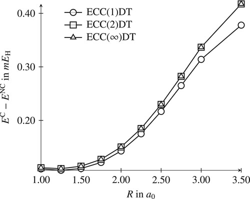
The energy curves of the canonical models C-ECC(n)SD are identical to the non-canonical NC-ECC(n)SD ones and are thus not presented here. However, the results differ if excitation-rank incomplete truncation schemes are employed. For instance, in canonical ECC(n)DT, singles amplitudes are effectively generated from doubles and triples amplitudes, while these are absent in the non-canonical model. This effect has been studied on the potential curve of the HF molecule and is depicted in Figure : The generation of singles amplitudes entails that the canonical computation is lower in energy, in particular towards the multireference region where these contribute significantly to the wave function expansion. This depends, however, on the role of the singles amplitudes in the wave function: In test computations on the H model system a different trend was observed, consistent with the diminished importance of singles in the wave function (vide infra). Therefore, we cannot conclude that the canonical coordinates are consistently better when unconventional truncations are used.
Figure 1. Difference between a canonical and a non-canonical ECC(n)DT computation for the potential curve of HF.
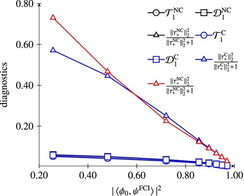
In order to investigate the effect of using different coordinates in ECC(n)SD computations, we calculated a set of CC diagnostics which are often used to assess the quality of CC computations [Citation40,Citation41]. These are based on the largest singular value () and Frobenius norm (
) of the matrix representation of the singles amplitudes. (Equivalently,
, the sum of the squares of the singles amplitudes, with N the number of correlated electrons.) Although diagnostics based on doubles amplitudes are preferred, they are not as available in implementations as are the singles-based variants [Citation42]. Additionally, we computed the diagnostic
which involves all the amplitudes. This choice can be motivated from monotonicity arguments and will be discussed in a forthcoming paper.
The values have been computed for truncation schemes . Since the trends are very similar, only the data for n = 1 is presented for HF and H
. For N
, we focus on the results for n = 2, because the quadratic model is well-known to be a better approximation to full CI compared to standard CCSD in this case [Citation16] (cf. line starting upper left with triangle markers in Figure ). We stress, that even if the NC-ECC(1)SD and C-ECC(1)SD (which is standard CCSD) are equivalent, the singles amplitudes in their respective parameterisations differ, producing different values for the diagnostics. Figure shows the diagnostics correlated with the multireference character for the HF potential curve, in Figures and values for the H
model and the N
molecule are shown, respectively. In both H
and N
, electron correlation is dominated by doubles amplitudes, as can be seen from the small values of the singles-based diagnostics. Since the reparameterisation of the amplitudes in the canonical model does not affect the amplitudes of highest excitation rank, the difference between the NC-ECC(n)SD and C-ECC(n)SD amplitude vectors is negligible. This is different for the HF case. Here, the amplitude norms of the canonical models are consistently smaller than the non-canonical variants, indicating that the wave function parameterisation is more compact.
Figure 2. Comparison of CC diagnostics of the C-ECC(1)SD and NC-ECC(1)SD model for the HF potential curve correlated with the multireference character.
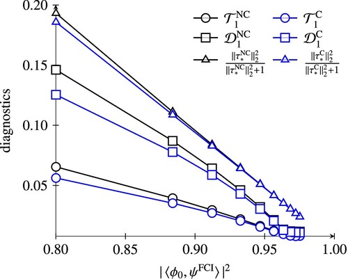
Figure 3. Comparison of CC diagnostics of the C-ECC(1)SD and NC-ECC(1)SD model for the H potential curve correlated with the multireference character.
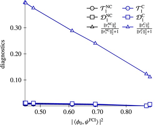
Figure 4. Comparison of CC diagnostics of the C-ECC(2)SD and NC-ECC(2)SD model (lower set of five curves, almost on top of each other) for the N potential curve correlated with the multireference character. The red curve shows diagnostics for NC-ECC(1)SD, indicating the inferiority of this model in the multireference region.
Our numerical experiments suggest, that for excitation-rank incomplete models, the canonical map generates effectively an excitation-rank complete parameterisation, but does not necessarily yield significantly better results. Concerning the a priori excitation-rank complete models, it has been found that the canonical parameterisation can be more compact compared to the non-canonical one, a desired property for post-Hartree–Fock methods. In particular, it may be useful to consider using canonical coordinates for diagnostics, even for well-established numerical codes using standard CC formalism.
5. Concluding remarks
In this article, we formulated basic error estimates for a class of exact models, defined in terms of replacing, in Arponen's ECC method, the exact exponential of the dual cluster operator with an n-th Taylor polynomial, the canonical C-NCC(n) models and the non-canonical NC-ECC(n) models. The central result was a coordinate-transformation theorem, Theorem 3.1, that gives error estimates for any method that can be described as a coordinate transformation of ECC theory. Notably, these results guarantee asymptotically quadratic error estimates for the ground-state energy of all models, under certain mild conditions.
Apart from Theorem 3.1, a basically self-contained mathematical framework for local error analysis of coupled-cluster methods was presented. This was based on Arponen's bivariational principle and basic results from nonlinear monotone operator theory, i.e. Zarantonello's theorem. Also central was our prior analysis of Arponen's extended coupled-cluster method in its non-canonical formulation.
The methods covered by our analysis include standard CC theory, quadratic CC theory [Citation18,Citation19], the perfect-pairing hierarchy [Citation20] for approximating CASSCF, also in its quadratic version [Citation19], and, Arponen's canonical ECC method. The computational cost of the (N)C-ECC methods truncated with the standard singles, doubles, etc., scheme, are expensive: already the nonlinear terms in
pushes the cost beyond standard CC theory when higher than doubles are considered. However, having obtained exact mathematical characterisations of the hierarchies of methods is an important first step in producing cheaper and more reliable methods compared to standard CC. One such approach could be similar to the CC2 method of Christiansen and coworkers [Citation43], where the cost of CCSD is reduced from
to
,
being the system size.
The error estimates are not optimal for many methods. A direct analysis of canonical ECC would probably provide the most optimistic analysis for all the C-ECC(n) methods, due to the doubly linked structure and the equivalence of excitation-rank complete Galerkin discretisations.
Finally, we performed some simple numerical experiments, focusing on the possibility of using canonical coordinates in place of the usual CC amplitudes when doing diagnostic estimates on CC calculations on systems with multireference character. Our preliminary findings support the hypothesis that the canonical coordinates are more compact compared to the usual coordinates, providing more accurate diagnostics.
An interesting extension of the present work would be to study truncations where singles-amplitudes are replaced by orbital rotations, either unitary or biorthogonal, as in the QCC and PP approaches, or the non-orthogonal orbital optimised coupled-cluster method of Pedersen and coworkers. [Citation44]. Moreover, the complete-active space coupled-cluster method by Adamowicz and coworkers [Citation32] fits the present scheme. It is also known that quadratic CC and ECC in general are quite good at reproducing multireference character, while standard single-reference CC is quite poor at this. Thus, a modified analysis of the ECC method that includes multireference assumptions, such as the steerable CAS-ext gap of Ref. [Citation34], could potentially lead to a deeper understanding of how CC methods generally behave in the presence of static correlation.
Acknowledgments
The authors are thankful to M. A. Csirik for useful comments.
Disclosure statement
No potential conflict of interest was reported by the authors.
Additional information
Funding
References
- J.S. Arponen, Ann. Phys. 151 (2), 311–382 (1983). doi:10.1016/0003-4916(83)90284-1.
- J.S. Arponen, R.F. Bishop and E. Pajanne, Phys. Rev. A 36, 2519–2538 (1987). doi:10.1103/PhysRevA.36.2519.
- T. Helgaker and P. Jørgensen, Adv. Quant. Chem. 19, 183–245 (1988). doi:10.1016/S0065-3276(08)60616-4.
- J. Hubbard, Proc. Roy. Soc. A: Math. Phys. Eng. Sci. 240 (1223), 539–560 (1957). doi:10.1098/rspa.1957.0106.
- F. Coester, Nucl. Phys. 7, 421–424 (1958). doi:10.1016/0029-5582(58)90280-3.
- F. Coester and H. Kümmel, Nucl. Phys. 17, 477–485 (1960). doi:10.1016/0029-5582(60)90140-1.
- J. Paldus, in Theory and Applications of Computational Chemistry: The First Forty Years, edited by C.E. Dykstra, G. Frenking, K.S. Kim, and G.E. Scuseria (Elsevier, Edinburgh, London, Amsterdam, 2005), Chap. 7, p. 115.
- R.J. Bartlett and M. Musiał, Rev. Mod. Phys. 79 (1), 291–352 (2007). doi:10.1103/RevModPhys.79.291.
- G. Hagen, T. Papenbrock, M. Hjorth-Jensen and D.J. Dean, Rep. Prog. Phys. 77 (9), 096302 (2014). doi:10.1088/0034-4885/77/9/096302.
- K. Emrich and J.G. Zabolitzky, in Recent Progress in Many-Body Theories, edited by H. Kümmel and M.L. Ristig (Springer, Berlin, Heidelberg, 1984), pp. 271–278.
- B.H.J. McKellar, C.R. Leonard and L.C.L. Hollenberg, Int. J. Mod. Phys. B 14, 2023–2037 (2000). doi:10.1142/S0217979200001151.
- L.S. Cederbaum, O.E. Alon and A.I. Streltsov, Phys. Rev. A 73 (4) (2006). doi:10.1103/PhysRevA.73.043609.
- J.S. Arponen, J. Phys. G: Nucl. Phys. 8, L129 (1982). doi:10.1088/0305-4616/8/8/004.
- J.S. Arponen, R.F. Bishop and E. Pajanne, Phys. Rev. A 36, 2539–2549 (1987). doi:10.1103/PhysRevA.36.2539.
- R.F. Bishop, Theor. Chim. Acta 80, 95–148 (1991). doi:10.1007/BF01119617.
- B. Cooper and P.J. Knowles, J. Chem. Phys. 133 (234102), 20120 (2010). doi:10.1063/1.3520564.
- F.A. Evangelista, J. Chem. Phys. 134 (22), 224102 (2011). doi:10.1063/1.3598471.
- T. Van Voorhis and M. Head-Gordon, Chem. Phys. Lett. 330, 585–594 (2000). doi:10.1016/S0009-2614(00)01137-4.
- E.F.C. Byrd, T. Van Voorhis and M. Head-Gordon, J. Phys. Chem. B 106 (33), 8070–8077 (2002). doi:10.1021/jp020255u.
- S. Lehtola, J. Parkhill and M. Head-Gordon, J. Chem. Phys. 145, 134110 (2016). doi:10.1063/1.4964317.
- E. Zarantonello, Technical Report 160 (U.S. Army Math. Res. Centre, Madison, WI, 1960).
- E. Zeidler, Nonlinear Functional Analysis and Its Application II/B (Springer, New York, Heidelberg, Berlin, 1990).
- A. Laestadius and S. Kvaal, SIAM J. Numer. Anal. 56 (2), 660–683 (2018). doi:10.1137/17M1116611.
- A. Laestadius and F.M. Faulstich, Mol. Phys. 117 (17), 2362–2373 (2019). doi:10.1080/00268976.2018.1564848.
- R. Schneider, Numer. Math. 113, 433–471 (2009). doi:10.1007/s00211-009-0237-3.
- T. Rohwedder, ESAIM: Math. Mod. Num. Anal. 47, 421–447 (2013). doi:10.1051/m2an/2012035.
- T. Rohwedder and R. Schneider, ESAIM: Math. Mod. Num. Anal. 47, 1553–1582 (2013). doi:10.1051/m2an/2013075.
- R.P. Feynman, Phys. Rev. 56 (4), 340–343 (1939). doi:10.1103/PhysRev.56.340.
- M. Reed and B. Simon, Methods of Modern Mathematical Physics I: Functional Analysis (Academic Press, San Diego, New York, 1980).
- K. Schmüdgen, Unbounded Self-adjoint Operators on Hilbert Space. Graduate Texts in Mathematics (Springer, Dordrecht, Heidelberg, 2012).
- C. Hättig, W. Klopper, A. Köhn and D.P. Tew, Chem. Rev. 112, 4–74 (2012). doi:10.1021/cr200168z.
- L. Adamowicz, J.-P. Malrieu and V.V. Ivanov, J. Chem. Phys. 112 (23), 10075–10084 (2000). doi:10.1063/1.481649.
- K. Kowalski, J. Chem. Phys. 148, 094104 (2018). doi:10.1063/1.5010693.
- F. Faulstich, A. Laestadius, S. Kvaal, Ö. Legeza and R. Schneider, SIAM J. Num. Anal. 57, 2579 (2019). doi:10.1137/18M1171436.
- T. Kinoshita, O. Hino and R.J. Bartlett, J. Chem. Phys. 123 (7), 074106 (2005). doi:10.1063/1.2000251.
- F.M. Faulstich, M. Máté, A. Laestadius, M.A. Csirik, L. Veis, A. Antalik, J. Brabec, R. Schneider, J. Pittner, S. Kvaal and Ö. Legeza, J. Chem. Theor. Comp. 15 (4), 2206–2220 (2019). doi:10.1021/acs.jctc.8b00960.
- E. Zeidler, Nonlinear Functional Analysis and Its Application I (Springer, New York Heidelberg Berlin, 1986).
- A. Engels-Putzka and M. Hanrath, Mol. Phys. 107 (2), 143–155 (2009). doi:10.1080/00268970902724922.
- K. Jankowski, L. Meissner and J. Wasilewski, Int. J. Quant. Chem. 28 (6), 931–942 (1985). doi:10.1002/qua.v28:6. doi: 10.1002/qua.560280622
- T.J. Lee and P.R. Taylor, Int. J. Quant. Chem. 36 (S23), 199–207 (1989). doi:10.1002/qua.v36:23+. doi: 10.1002/qua.560360824
- C.L. Janssen and I.M.B. Nielsen, Chem. Phys. Lett. 290 (4), 423–430 (1998). doi:10.1016/S0009-2614(98)00504-1.
- W. Jiang, N.J. DeYonker and A.K. Wilson, J. Chem. Theor. Comp. 8 (2), 460–468 (2012). doi:10.1021/ct2006852 PMID: 26596596.
- O. Christiansen, H. Koch and P. Jørgensen, Chem. Phys. Lett. 243, 409–418 (1995). doi:10.1016/0009-2614(95)00841-Q.
- T.B. Pedersen, B. Fernández and H. Koch, J. Chem. Phys. 114, 6983 (2001). doi:10.1063/1.1358866.
Appendix. Proofs of main results
In this appendix all our proofs have been collected and are given in the same order as the corresponding results have appeared above. We will only present a partial proof of Theorem 2.1, as the proofs of points (1) and (2) are standard, and can be found in, e.g. Ref. [Citation22].
Proof
Proof of Theorem 2.1
For point (3), we note that F is locally Lipschitz continuous as a consequence of being smooth, which together with strong monotonicity makes points (1) and (2) applicable. The remaining argument follows [Citation23] closely (where the case
was treated). First, by assumption of R,
and
are equivalent to
and
, respectively (note that R commutes with
). Now, Taylor expanding
around
and evaluating at
gives
By the smoothness of
, there exists a constant
such that
Further, the fact that on U we can control the higher-order terms by the quadratic one, we have
Using Equation (Equation8
(8)
(8) ) gives the full statement in Equation (Equation9
(9)
(9) )
Proof
Proof of Theorem 3.1
With the flipped gradient and
, we obtain
In the sequel, we omit the specification of the spaces in the dual pairing.
Let be such that
, i.e.
. Since F is smooth, local strong monotonicity of F is equivalent to
(the set of bounded linear operators) being coercive, i.e. there exists an
such that
where
is defined by the first equality. (The constant η in Equation (Equation6
(6)
(6) ) approaches
as the ball U given in Theorem 2.1 of the local strong monotonicity approaches a point.) To see this, we find an expression for
in terms of the energy map,
(A1)
(A1) Here
is the directional derivative in the direction of X such that
where
. By choosing ε small enough, Equation (EquationA1
(A1)
(A1) ) and strong monotonicity gives the coercivity claim. The logical implication also goes in the reverse direction. (This will be used below.)
Recall that and that
denotes the flipped gradient of
. We use that
is locally strongly monotone at
if and only if
is coercive, i.e.
for some
and all
. A straightforward application of the chain rule now gives
We note that this is almost . Indeed,
(A2)
(A2) In particular, if
then the last term vanishes in the utmost right-hand side of Equation (EquationA2
(A2)
(A2) ), and we obtain monotonicity of
but with a modified constant.
In the case where , we write
, and note that
. We obtain,
(A3)
(A3) Here, we used that θ has a smooth inverse, implying
, and that
.
Proof
Proof of Corollary 3.2
We consider the Jacobian of the coordinate map, which on block form reads
(A4)
(A4) For the map
(see Equation (Equation17
(17)
(17) )), we first observe that by definition,
from which it follows, by taking the logarithm and expanding the logarithm around
, which is a finite Taylor series,
We obtain
(A5)
(A5) For the map
we have, using the chain rule,
(A6)
(A6) Here,
is the linear transformation on
such that
(see Equation (Equation12
(12)
(12) )), i.e.
can be expressed in terms of the matrix representation of
,
(A7)
(A7) We have
, and
. For both maps, the Jacobian of the coordinate transformation at the critical point
becomes
with
. Applying Theorem 3.1(2), the local strong monotonicity follows, and by Theorem 2.1, quasi-optimality of the truncated solutions and a quadratic error estimate.