
 ?Mathematical formulae have been encoded as MathML and are displayed in this HTML version using MathJax in order to improve their display. Uncheck the box to turn MathJax off. This feature requires Javascript. Click on a formula to zoom.
Abstract
Recently, we determined the detailed energy level structure of the ,
and
states of AlF that are relevant to laser cooling and trapping experiments [Truppe et al., Phys. Rev. A. 100 (5), 052513 (2019)]. Here, we investigate the
state of the AlF molecule. A rotationally resolved (1 + 2)-REMPI spectrum of the
band is presented and the lifetime of the
state is measured to be 190(2) ns. Hyperfine-resolved, laser-induced fluorescence spectra of the
and the
bands are recorded to determine fine- and hyperfine structure parameters. The interaction between the
and the nearby
state is studied and the magnitude of the spin–orbit coupling between the two electronic states is derived using three independent methods to give a consistent value of 10(1) cm
. The triplet character of the A state causes an
loss from the main A−X laser cooling cycle below the 10
level.
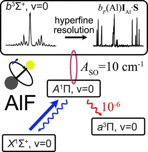
GRAPHICAL ABSTRACT
1. Introduction
Polar molecules, cooled to low temperatures, have wide-ranging applications in physics and chemistry [Citation1, Citation2]. Recently, we identified the AlF molecule as an excellent candidate for direct laser cooling to low temperatures and with a high density [Citation3]. AlF has one of the strongest chemical bonds known (6.9 eV), can be produced efficiently, and captured and cooled in a magneto-optical trap using any Q-line of its strong band near 227.5 nm. Subsequent to trapping and cooling on the strong A−X transition, the molecules may be cooled to a few µ K on any (narrow) Q-line of the spin-forbidden
band. To laser-cool AlF successfully, it is essential to study the detailed energy level structure of the molecule, to measure the radiative lifetime of the states involved and to investigate and quantify the potential decay channels to states that are not coupled by the cooling laser, i.e. losses from the optical cycle.
For nearly a century, spectroscopists have been interested in the AlF molecule, in part due to its similarity to the much-studied CO and N molecules. AlF is also important to the astrophysics community and it has been detected in sunspots, stellar atmospheres, circumstellar envelopes and proto-planetary nebulae [Citation4, Citation5]. Moreover,
AlF was the first radioactive molecule to be discovered in space [Citation6]. AlF has been the subject of theoretical studies using ab initio quantum chemistry to determine radiative lifetimes, dipole moments and potential energy curves for its electronic states [Citation7–10]. Precise spectroscopic parameters for AlF are useful for future astrophysical observations and new spectroscopic studies of electronic states can serve as a benchmark for quantum chemistry calculations.
In this paper, we present rotationally resolved optical spectra of the band and demonstrate state-selective ionisation of
molecules via (1 + 2)-resonance-enhanced multi-photon ionisation (REMPI). Pulsed excitation followed by delayed ionisation with a KrF excimer laser is used to determine the radiative lifetime of the
state. Next, high-resolution, cw laser-induced fluorescence (LIF) spectra of the
band are presented. The hyperfine structure in the
state is resolved and precise spectroscopic constants for the b state are determined. Laser-induced fluorescence spectra, recorded using a cw laser to drive rotational lines of the
band, allow us to reduce the uncertainty in the spin–orbit constant A and the spin–spin interaction constant λ of the
state by nearly two orders of magnitude. A fraction of the excited state molecules decay on the
bands to the ground state. This is caused by the spin–orbit coupling of the
state with the nearby
state. This perturbation of the
state and the
state is analysed in detail as it also induces a small loss channel for the strong A−X cooling transition.
2. Previous work
In 1953, Rowlinson and Barrow reported the first observation of transitions between triplet states in AlF by recording emission spectra from a hollow-cathode discharge [Citation11]. In the following decades, new triplet states were identified and characterised in more detail [Citation12–16]. Kopp and Barrow analysed the interaction of the state with the nearby
state and thereby determined the term energy of the triplet states relative to the singlet states [Citation16]. A comprehensive study of the electronic states and the interaction between the singlet and triplet states followed [Citation17]. In 1976, Rosenwaks et al. observed the
transition directly in emission [Citation18] at the same time as Kopp et al. did in absorption [Citation19]. Both studies confirmed the singlet-triplet separation determined from the earlier perturbation analysis.
The hyperfine structure of the rotational states in was partly resolved and analysed by Barrow et al. [Citation17]. Their low-resolution spectra (typical linewidth of 0.05 cm
) showed a triplet structure, which they ascribed to magnetic hyperfine effects of the
Al nucleus, whose nuclear spin is
. A more detailed analysis of both the fine and hyperfine structure in the triplet states was presented by Brown et al. in 1978 [Citation20]. The hyperfine structure was partially resolved and they determined values for the Fermi contact parameter
, the electron spin–spin interaction parameter λ, and the spin–rotation parameter γ.
We have recently reported on the detailed energy level structure of the ,
and
states in AlF [Citation3]. That study resolves the complete hyperfine structure, including the contribution due to fluorine nuclear spin, in all three states. The energy levels in
and in the three Ω manifolds of the metastable
state were measured with kHz resolution; this allowed us to determine the spectroscopic constants precisely and study subtle effects, such as a spin–orbit correction to the nuclear quadrupole interaction of the Al nucleus.
3. Rotational structure of the  band and the radiative lifetime of the state
To study the b−a transition, the molecules must first be prepared in the state. Previously, we described this state and the a−X transition in detail [Citation3]. The hyperfine structure in
is small and for the purpose of this study, the ground state is comprised of single rotational levels with energies given by
.
The angular momentum coupling in the state of AlF is well-described by Hund's case (a). The energy levels are labelled by the total angular momentum (excluding hyperfine interaction)
, with
the rotational angular momentum of the rigid nuclear framework, and
and
the total orbital and spin angular momenta of the electrons, respectively. Both
and
are not well defined. However, their projection onto the internuclear axis
and
and the total electronic angular momentum along the internuclear axis
are well defined. The spin–orbit interaction leads to three fine structure states with
, labelled with
,
and
, in order of increasing energy, corresponding to the states
,
and
. The splitting between the Ω manifolds is determined by A, the electron spin–orbit coupling constant and the spin–spin interaction coupling constant λ. Each Ω has its own rotational manifold with energies
, where the rotational constant B is slightly different for each Ω manifold.
The state is well-described by Hund's case (b), for which
couples to the rotation
to form
. The rotational energy levels follow
. For Σ electronic states
and the total angular momentum (without hyperfine interaction) is
. The combined effect of the spin–rotation interaction
and the spin–spin interaction
splits each rotational level N>0 of
into three J-levels; these components are labelled
,
and
with quantum numbers J = N + 1, J = N and J = N−1, respectively.
Following the convention of Brown et al. [Citation21] the parity states can be labelled by e and f, where e levels have parity and f labels have parity
. All rotational levels of the
state are e-levels, while in the
state, all
levels are e-levels, while
and
are f-levels. In the
state, each J-level has an e and an f component due to Λ-doubling.
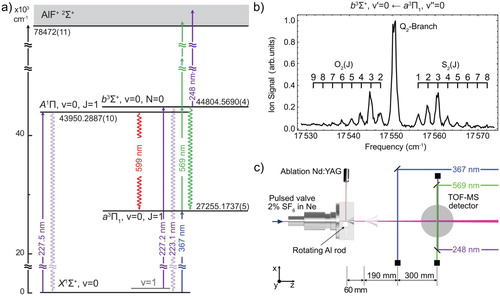
Figure (a) shows the energy level diagram of the electronic states relevant to this study, together with a rotationally resolved spectrum of the band in (b), and a sketch of the experimental setup in (c), which is similar to the one reported previously [Citation3]. The molecules are produced by laser-ablating an aluminium rod in a supersonic expansion of 2% SF
seeded in Ne. After passing through a skimmer, the ground-state molecules are optically pumped to the metastable
state by a frequency-doubled pulsed dye laser using the Q-branch of the
band. For this, 367 nm radiation with a bandwidth of 0.1 cm
and pulse energy of 6 mJ in a beam with a
waist radius of about 2 mm is used. The Q-branch of this transition falls within this bandwidth. Therefore, many rotational levels in the metastable
state are populated simultaneously. Via the Q-branch, only the f-levels in
are populated. Alternatively, if the molecules are optically pumped to the metastable state using spectrally isolated R or P lines, only the e-levels are populated. Further downstream, at z = 55 cm from the source, the molecular beam is intersected with light from a second pulsed dye laser tuned to the
transition near 569 nm. For pulse energies exceeding 6 mJ (unfocused, with an
waist radius of about 5 mm), this laser transfers population to the
state and subsequently ionises the molecules by having them absorb two more photons from the same laser. Such a one-colour (1 + 2)-REMPI scheme using an unfocused laser beam is very uncommon. However, AlF has numerous electronically excited states that lie one photon-energy above the b state energy, strongly enhancing the non-resonant two-photon ionisation probability. The ions are mass-selected in a short time-of-flight mass spectrometer (TOF-MS) and detected using micro-channel plates. The TOF-MS voltages are switched on shortly after the ionisation laser fires; this way ionisation occurs under field-free conditions and the states have a well-defined parity. The (1 + 2)-REMPI scheme uses low-energy photons and an unfocused laser beam, which has the benefit of producing a mass spectrum with only a single peak, corresponding to AlF. The spectrum, displayed in Figure (b), shows the ion signal as a function of the REMPI laser frequency. The spectral lines are labelled by
, where
, as the quantum number J is not well-defined in the b state, vide infra. Since only the f-levels of the
state are populated, the spectrum consists of
, i.e. O, Q and S branches.
Figure 1. (a) Electronic energy level scheme of the relevant states of AlF. The transitions used for laser excitation are shown as solid arrows. The laser-induced fluorescence used for detecting the molecules is indicated by downward wavy arrows. The indicated energies are the gravity centres of the respective states in the absence of hyperfine structure. (b) (1 + 2)-REMPI spectrum of the band. The
state is populated via the Q-branch of the
band using a frequency-doubled pulsed dye laser. (c) Schematic of the experimental setup used for the determination of the lifetime of the
state.
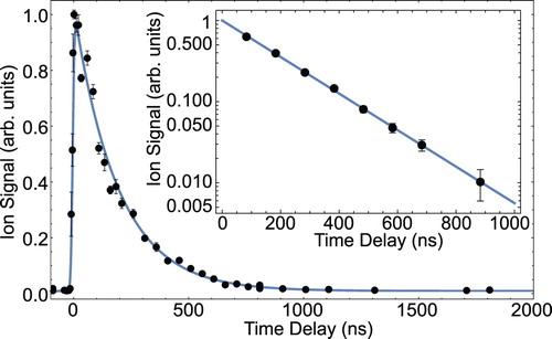
To determine the radiative lifetime of the state, we reduce the pulse energy of the
excitation laser to about 1 mJ. At pulse energies below 2 mJ, the
molecules are excited to the b state, but are not ionised via (1 + 2)-REMPI. Instead, a KrF excimer laser is used to ionise the b state molecules with a single 248 nm photon and pulse energy of about 3 mJ. The radiative lifetime of the
state is measured by varying the time-delay between excitation and ionisation [Citation22]. The determination of radiative lifetimes in the range of 20 ns to 1 μs is relatively straightforward, because it is longer than the laser pulse duration, but short enough so that the molecules do not leave the detection region. Figure shows the ion signal (black dots) as a function of the time-delay with
standard error bars. The blue line is a fit to the data using the model
, where
is the complementary error function, C and
are fit parameters,
is the lifetime of the
state and σ is the measured, combined pulse-width of the excitation and ionisation laser. In this model, the lifetime
ns is fixed to the value determined from a linear fit to the semi-log plot shown in the inset. In 1988, Langhoff et al. calculated an approximate radiative lifetime of the
state of 135 ns [Citation8], considerably shorter than the measured lifetime.
Figure 2. Measurement of the radiative lifetime of the state. First, the ground-state molecules are optically pumped to the
state via the two-colour excitation scheme described in the text. The population in the
state is probed by single-photon ionisation using a KrF excimer laser, followed by TOF-MS detection. The black dots show the AlF
ion signal as a function of the time-delay between excitation and ionisation. The blue line is a fit to the data using the model described in the text. The inset shows a semi-log plot of a second measurement for eight specific time delays. A linear fit to the data gives a b state lifetime of 190(2) ns (colour online only).
4. The fine and hyperfine structure of the state
Aluminium and fluorine have a nuclear spin of and
, respectively. Following the description of Brown et al. [Citation20] and including the magnetic interaction of the fluorine nuclear spin, the effective Hamiltonian reads
(1)
(1) where λ is the spin–spin interaction constant and γ the spin–rotation interaction constant. The parameters
and
describe the Fermi contact interaction for the aluminium and fluorine nucleus, respectively,
and
the dipolar interaction, and
the electric quadrupole interaction of the Al nucleus.
In the state of AlF, the Fermi contact interaction
between the nuclear spin of aluminium and the electronic spin angular momentum is strong compared to the spin–rotation interaction [Citation20]. The coupling case approximates
. The N = 0 level has only one spin-component for which J = N + S = 1; this J = 1 level is split into three components due to the aluminium nuclear spin, each of which is again split by the nuclear spin of fluorine. This results in a total of six F levels. For N>0, J is not well defined and it is useful to introduce an intermediate angular momentum
(see Figure ).
then couples to
which results in three sets of sub-levels, with quantum numbers
and 7/2, each of which contains the closely spaced stacks of
,
and
levels. Each of these levels is again split by the interaction with the fluorine nuclear spin to give the total angular momentum
. For N = 1, 2 and 3 this results in a total of 18, 28 and 34 F levels, respectively. For
the number of F levels reaches its limit of 36.
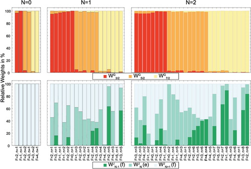
Figure 3. Relative weights and
of the
and
basis wave functions in the eigenfunctions
of the energy levels in the three lowest rotational states of the
state. The weights are obtained by projecting the eigenstate of the Hamiltonian onto the basis wave function
and
, respectively. G can take the values 3/2, 5/2 and 7/2 and J can be
or N + 1. The energy levels are described uniquely by the quantum numbers F, p and the index n. This analysis shows that G is a good quantum number for the description of any rotational level of the
state, while J only characterises the levels well for N = 0.
To determine the hyperfine energy levels of the state, we drive the
band near 227.2 nm with a cw laser and detect the b−a fluorescence at 569 nm. The spectrum of this transition directly reflects the energy level structure in the
state, because the hyperfine structure of the
state is smaller than the residual Doppler broadening in the molecular beam. The wavelength required to drive this transition is close to that of the
band near 227.5 nm, for which we have a powerful UV laser system installed.
The transition is spin-forbidden and the overlap of the vibrational wave functions is poor, with a calculated Franck–Condon factor of 0.02. However, the transition becomes weakly allowed due to the spin–orbit interaction between the
and the nearby
state. In Section 7, this interaction will be discussed in more detail. To compensate for the weak transition dipole moment, we use a high excitation laser intensity of up to 75 mW in a laser beam with an
waist radius of 0.6 mm. The resulting laser-induced fluorescence occurs mainly on the dipole-allowed b−a transition near 569 nm. The far off-resonant fluorescence allows us to block scattered laser light with a bandpass filter and to record background-free spectra. To increase the number of molecules in
, we use a cryogenic helium buffer gas source, instead of the supersonic molecular beam introduced in the previous section. Figure shows a sketch of the experimental setup that is used for this measurement.
Figure 4. Schematic of the experimental setup used to measure the fine and hyperfine structure of the state. AlF molecules are produced in a cryogenic helium buffer gas source. The molecular beam is intersected with UV laser light from a frequency-quadrupled cw titanium sapphire laser. The molecules are excited on the weak, spin-forbidden
transition. The laser-induced fluorescence occurs mainly on the
transition near 569 nm and is imaged onto a PMT.
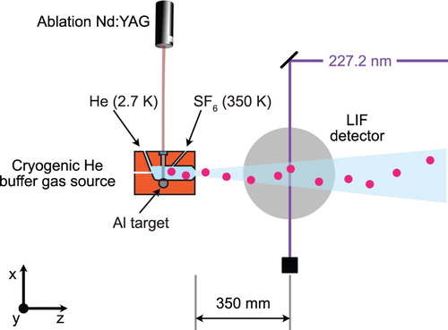
The design of this source is similar to the one described in [Citation23–25]. A pulsed Nd:YAG laser ablates a solid aluminium target in the presence of a continuous flow of 0.01 sccm room-temperature SF gas, which is mixed with 1 sccm of cryogenic helium gas (2.7 K) inside a buffer gas cell. The hot Al atoms react with the SF
and form hot AlF molecules, which are subsequently cooled through collisions with the cold helium atoms. Compared to the supersonic molecular beam, this source delivers over 100 times more AlF molecules per pulse in the rovibronic ground-state to the detection region. The forward velocity of the molecules is four times lower. To increase the number of molecules in
, we increase the pulse energy and repetition rate of the ablation laser, increase the temperature of the SF
gas to 350 K and increase its mass flow rate to 0.1 sccm. At z = 35 cm the molecules interact with cw UV laser light to drive the
transition near 227.2 nm. The laser light is produced by frequency-doubling the output of a cw titanium sapphire laser twice. The laser-induced fluorescence passes through an optical filter to block scattered light from the excitation laser and is imaged onto a photomultiplier tube (PMT). The photo-current is amplified and acquired by a computer. The wavelength of the excitation laser is recorded with an absolute accuracy of 120 MHz using a calibrated wavemeter (HighFinesse WS8-10).
Figure shows the recorded spectra reaching the three lowest N levels in the b state. The panels demonstrate the increasing complexity of the hyperfine structure with increasing N. The three spectra allow us to measure the rotational constant of the b state. Gaussian lineshapes are fitted to the experimental spectra to determine the line-centres. We then fit the eigenvalues of the hyperfine Hamiltonian to the measured energy levels with the spectroscopic parameters as fit parameters. We assign a total of 48 lines and the standard deviation of the fit is 11 MHz. The best-fit parameters together with their standard deviations are summarised in Table . is the pure vibronic energy of
, i.e. the energy of the N = 0 level in the absence of spin, fine and hyperfine splitting. This is referenced to the J = 0 level of the
state by using the precise infrared emission lines of [Citation26] to determine the energy difference between the v = 0 and v = 1 level in the X state. The inverted spectra in Figure are simulated spectra using the spectroscopic parameters presented in Table and reproduce the measured spectra well. The Fermi contact parameter
for fluorine and the two hyperfine parameters
and
for the aluminium and fluorine nucleus, respectively, are determined for the first time. In previous, low-resolution studies, the interaction of the fluorine nuclear spin has been neglected. However, we conclude that the magnitude of the interaction parameter for the two nuclei is comparable. This indicates that there is a significant electron density at both nuclei, which is in stark contrast to the situation in the
state. In the latter state, the Fermi contact term for the
F nucleus is about seven times smaller than for the
Al nucleus [Citation3]. The Fermi contact parameter for the aluminium nucleus
and the spin–spin interaction parameter λ presented here are consistent with the previously determined values, but their uncertainty is reduced significantly. Table lists the energies of the relevant hyperfine levels in
with their respective magnetic g-factors. The weights of the
and
basis wave functions in the eigenfunctions of these energy levels are shown in Figure .
5. The transition
The b−a bands have a diagonal Franck–Condon matrix and the band has a Franck–Condon factor of 0.994. Its natural linewidth is 100 times smaller than the natural linewidth of the strong
transition near 227.5 nm. Laser cooling AlF molecules on the b−a transition could therefore reach temperatures far below the Doppler limit of the strong A−X transition. The vibrational branching to
is small and, if addressed with a repump laser, a molecule could scatter about 1000 photons before being pumped into
. However, the radiative decay from the b state to multiple J levels in all three spin–orbit manifolds of the a state is allowed. This results in a large number of rotational branches that must be addressed to close the optical cycle [Citation28]. In addition, the hyperfine structure in a is large compared to the linewidth of the transition. Both effects make laser cooling of AlF, using an optical transition in the triplet manifold very challenging. This is in stark contrast to the strong A−X transition, for which all Q-lines are rotationally closed and for which all hyperfine levels of a given rotational level in the X state lie within the natural linewidth.
Here, we demonstrate that laser-induced fluorescence spectroscopy of the transition can be used to efficiently detect
molecules with hyperfine resolution. In this section, we show that this method works well to detect molecules in all three Ω manifolds to improve two important spectroscopic constants of the
state: the spin–orbit (A) and spin–spin (λ) interaction parameter, which determines the relative spacing of the three Ω manifolds in
. The effective fine structure Hamiltonian is
(2)
(2) The interval between the
and
manifolds is approximately
, while the
and
manifolds are about
apart.
For this experiment, we use the supersonic molecular beam setup introduced in Section 3, with an additional LIF detector installed between the excitation region and the TOF-MS. After passing through the skimmer, the molecules are excited on a specific rotational line of the band to one of the three spin–orbit manifolds, using a frequency-doubled pulsed dye amplifier (PDA), which is seeded by a cw titanium sapphire laser. About 30 cm further downstream, a cw ring dye laser intersects the molecular beam orthogonally and is scanned over a rotational line of the
band. The laser frequency is stabilised and scanned with respect to a frequency-stabilised and calibrated HeNe reference laser (SIOS SL 03), using a scanning transfer cavity. The wavelength is recorded with an absolute accuracy of 10 MHz using the wavemeter, calibrated by the same HeNe laser.
Figure shows hyperfine-resolved LIF excitation spectra of the band. Figure (a) shows the hyperfine spectrum of the
lines. The positive parity Λ-doublet level of
has only two hyperfine components with total angular momentum quantum numbers F = 2 and F = 3 that are only split by about 3 MHz, much smaller than the residual Doppler broadening in the molecular beam. Therefore, this b−a spectrum directly reflects the energy level structure in the b state and is identical to the one of the b−X spectrum shown in Figure (b).
Figure 5. Direct measurement of the fine and hyperfine structure of the three lowest rotational levels in the state, i.e. for
in panel (c),
, in panel (b) and
in panel (a). The experimental data are shown in black, pointing up and the simulated spectra are shown in blue, pointing down. The spectra are centred at the gravity centre, i.e. the line position in the absence of hyperfine, spin--spin and spin--rotation interaction (colour online only).
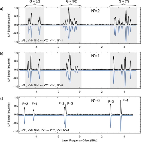
Figure 6. LIF excitation spectra of the b−a transition. Panels (a) and (b) show spectra of the and
transitions, respectively. The spectrum in the inset labelled UV is detected by recording the emission on the
bands as a function of the excitation frequency. (c) Hyperfine-resolved spectrum of the R
(1) line of the
band, showing the large hyperfine splitting in
. (d) Part of the hyperfine resolved spectrum of the
transition. The low (high) frequency part of this spectrum was recorded after excitation to the F = 4 (F = 5) component of the R
(1) line of the
transition. (a)–(d) The relevant energy level scheme is displayed next to each spectrum. Since J is not well-defined in the b state, the
transitions are labelled with
. The measured spectra are printed in black, while the simulated spectra are shown in blue and inverted (colour online only).
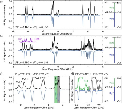
The spectrum of the transition, presented in Figure (b), shows a richer structure, and no longer directly reflects the energy level structure in the b state. The total span of the hyperfine splitting in the
level is about 500 MHz [Citation3], and contributes to the complexity of this spectrum.
Optical pumping to the state is challenging because the
transition of the
band is about 1000 times weaker than the corresponding
line to the
state. Only a small fraction of the ground-state molecules produced in the source is transferred to the
level, even with a PDA pulse energy of about 10 mJ in beam with a
waist radius of 1.5 mm. Figure (c) shows the R
line of the
band, recorded by scanning the seed laser of the frequency-doubled PDA, followed by (1 + 2)-REMPI and TOF-MS detection. The hyperfine structure in
is very large and it is possible to resolve six of the ten hyperfine levels using a narrow-band pulsed laser. This enables us to populate a specific hyperfine component of the
level, which is then followed by cw excitation to the b state and LIF detection. Figure (d) shows two LIF spectra that originate from two different hyperfine states in
, indicated by the two colours. The green spectrum originates from the
level and the grey spectrum from the
level. The line-centres are determined by fitting Gaussians to the spectral lines.
The hyperfine structure and Λ-doubling of the state has been investigated extensively in our previous study and is known to kHz precision [Citation3]. However, the constants A and λ of the
state could only be determined with an accuracy of about 200 MHz, due to the finite bandwidth of the pulsed laser and the lower accuracy of the wavemeter that was used in that study to measure the relative energy of the Ω manifolds. Here, we take advantage of the reduced linewidth in the cw LIF spectra of the b−a transition, in combination with the increased accuracy of our new wavemeter, to improve this measurement and therefore the spectroscopic constants A and λ. By using the hyperfine constants for the
state from reference [Citation3] in combination with the parameters for the b state, listed in Table , the b−a spectra can be simulated, and new values for A and λ are derived. The simulated spectra, using the full Hamiltonian, including the hyperfine interactions in both states are shown in Figure as blue, inverted curves. The uncertainty of the improved spectroscopic constants, listed in , is reduced by nearly two orders of magnitude compared to the ones presented previously [Citation3].
is the term energy of the a state in the absence of rotation, fine and hyperfine structure, calculated by using the term energy of the b state determined in the previous section. This means that the gravity centre, i.e. the position of the
level in the absence of hyperfine structure, relative to the
level is at 27255.1737(5) cm
.
Table 1. Experimentally determined spectroscopic constants of .
Table 2. Spectroscopic constants for the state of AlF, determined from a fit to the spectra.
It is also possible to record the LIF excitation spectra by detecting the weak UV fluorescence, on the bands which occurs predominantly at 223.1 nm. Part of the spectrum displayed in Figure (b) has also been recorded this way and is shown by the inset labelled ‘UV’. To measure the ratio of the emission occurring in the UV, relative to the emission occurring in the visible, we lock the excitation laser to the resonance indicated by the arrow in Figure (b) and average the signal over 1000 shots. To distinguish the two wavelengths, we use two different PMTs: a UV sensitive one with a specified quantum efficiency of
at 223.1 nm and negligible sensitivity for wavelengths >350 nm and a second PMT with a specified quantum efficiency of
at 569 nm that is sensitive in the range of 200–800 nm. The quantum efficiencies of the PMTs are taken from the datasheet and are not calibrated further. However, three identical UV PMTs give the same photon count rate to within 15% which we take as the systematic uncertainty. Both PMTs are operated in photon-counting mode, counting the number of UV and visible photons,
and
, respectively. The visible PMT is combined with a bandpass interference filter to block the UV fluorescence and a small amount of phosphorescence on the
transition near 367 nm. The measured transmission of the filter at 569 nm is 0.57. We combine the slightly different transmission through the imaging optics, the different detector efficiencies and the filter transmission into the total detection efficiencies
and
. Including these values, we measure a ratio of
(3)
(3) This is the result of multiple experimental runs with a statistical error that is significantly smaller than the uncertainty in the quantum efficiencies of the PMTs. An additional 20% systematic uncertainty is added to the total error budget because we do not correct for the spherical and chromatic aberration of the fluorescence detector. However, simulations using ray-tracing software show a typical difference in imaging efficiency for the two wavelengths of about 10%. The value for
is identical to the ratio of the Einstein A-coefficients for
and
emission, i.e.
=
. The specific level in the
state for which this ratio of Einstein A-coefficients is determined, is the positive parity level with N = 2, F = 4, n = 4 which is almost a pure f-level, with 42.3%
and 57.4%
character, and only 0.3%
character. The level is highlighted in bold in and Figure .
Table 3. Energies, E, of the hyperfine levels in , relative to the level, magnetic g-factors , rotational quantum number N, total angular momentum F and parity p.
6. The bands
To probe the amount of triplet wave function that is mixed into the state directly, we measure the ratio
of the number of fluorescence photons emitted on the
and on the
transition. The value for
is identical to the ratio of the Einstein A-coefficients for
and
emission, i.e.
=
. The value for
gives the loss from the main laser cooling cycle due to electronic branching to the
state. Previously, we measured this electronic branching ratio on the
bands indirectly to be at the
level, by comparing the absorption-strength of the
transition relative to the absorption-strength of the
transition [Citation3]. In that analysis, we only took into account the amount of singlet character in the wave function of the a state to deduce the strength of the
transition. We did not account for the (then unknown) amount of triplet character in the wave function of the A state due to the interaction of the A and b states, which, as we will see here, turns out to be the dominant effect.
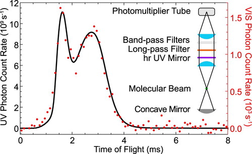
To measure such a small branching ratio directly, we use the buffer gas molecular beam source in combination with optical cycling on the Q(1) line of the A−X transition. The small amount of visible fluorescence is isolated from the strong UV fluorescence by a high-reflectivity UV mirror, which is transparent in the visible, in combination with a long-pass and two bandpass filters in front of the PMT. The transmission band of the filters is chosen such that only wavelengths that cover the transition are detected by the PMT. The mirror reduces the UV fluorescence that is incident on the spectral filters to the
level, suppressing their broadband phosphorescence when irradiated with UV light. The transmission of each optical element is measured individually at 227.5 nm and 599 nm, using laser light and a calibrated photodiode. The total detection efficiency, accounting for the transmittances and PMT responses becomes
for UV photons and
for visible photons in the range of 596–604 nm. The ratio of Einstein coefficients becomes
(4)
(4) where
and
are the number of photons detected in the visible and UV, respectively. A typical measurement is presented in Figure . The molecules are optically pumped on the Q(1) line of the 0-0 band of the A−X transition and the LIF is imaged and detected by two different PMTs. The majority of the fluorescence is emitted in the UV and imaged onto the UV sensitive PMT. The PMT is operated in current mode, which is converted into a voltage, amplified and read into the computer. We calibrate this PMT output voltage against the output of the PMT in photon-counting mode for low incident light intensities. The small fraction of the LIF that is emitted in the visible is shown as red dots. The two time-of-flight profiles are very similar, with the detected signal in the visible being
of the emission in the UV. By accounting for the different detection efficiencies for the two wavelengths the measured ratio is as given in Equation (Equation4
(4)
(4) ). The total uncertainty in this measurement is dominated by the systematic uncertainty in the quantum efficiency of the two PMTs and by the uncertainty in the imaging efficiency for the two wavelengths as described in Section 5.
Figure 7. The LIF emitted in the UV (227.5 nm, black) and VIS (599 nm, red) as a function of time when the UV laser frequency is locked to the Q(1) line of the transition. The inset shows the configuration of the fluorescence detector used for the VIS experiment (colour online only).
The measurement of is significantly more challenging than the measurement of
. This is because
is
times larger than
and the phosphorescence of the optical elements typically occurs red-shifted, i.e. in the wavelength range of the weak fluorescence in the visible. This is in contrast to the measurement of
, for which
is about 200 times smaller than
, and for which any background caused by the phosphorescence of the optical elements is absent.
We also measure the ratio of the visible to the UV fluorescence subsequent to excitation on the Q(1) line of the 1−1 band of the A−X transition. Since the level is energetically much closer to the
level, one might expect a significantly larger fraction of visible fluorescence. However, we find that the two ratios
are equal to within the 15% uncertainty of the measurement.
7. Spin–orbit interaction between the and states
The observation of the and of the
intersystem bands reported here indicates that the wave function of the b state of AlF contains a fraction of singlet character and that the A state contains a fraction of triplet character. This is due to the spin–orbit interaction of the b state with the nearby
state. Figure shows the potential energy curves for the lowest singlet and triplet electronic states of AlF. The inset shows a more detailed view of the
and
states with their vibrational levels indicated. For low vibrational quantum numbers, the vibrational level
in the b state lies slightly above the vibrational level
in the A state. The energy difference between
and
decreases with increasing vibrational quantum numbers until the levels have just crossed and are nearly degenerate at
(
), leading to a large perturbation of the rotational energy levels. This interaction has already been analysed by Barrow et al. in 1974, who introduced the parameter
to describe the effect of the spin–orbit interaction of specific pairs of vibrational levels, i.e. of
and 6 with
and 5, respectively [Citation17]. They used the observed perturbation to determine the energy of the triplet manifold relative to the singlet manifold with an accuracy of 0.05 cm
.
Figure 8. Potential energy curves for the lowest singlet and triplet electronic states of AlF, using precise Expanded Morse Oscillator (EMO) functions. We obtain these EMO potentials by fitting to the point-wise RKR potentials generated by LeRoy's program [Citation29] and adjust the parameters to predict the vibrational levels with a high accuracy of 0.05 cm (using the non-perturbed or de-perturbed values from the appendix from [Citation17] and from [Citation30]). These potentials are much more precise than the simple Morse model we use in Section 7, but do not allow us to treat the two electronic states independently to extract the spin–orbit interaction. Ab initio calculations indicate that the
state has a barrier in the region marked with a flash, which cannot be reproduced with our EMO potentials. The inset shows a more detailed view of the
and
potentials, with the vibrational levels indicated.
![Figure 8. Potential energy curves for the lowest singlet and triplet electronic states of AlF, using precise Expanded Morse Oscillator (EMO) functions. We obtain these EMO potentials by fitting to the point-wise RKR potentials generated by LeRoy's program [Citation29] and adjust the parameters to predict the vibrational levels with a high accuracy of 0.05 cm−1 (using the non-perturbed or de-perturbed values from the appendix from [Citation17] and from [Citation30]). These potentials are much more precise than the simple Morse model we use in Section 7, but do not allow us to treat the two electronic states independently to extract the spin–orbit interaction. Ab initio calculations indicate that the A1Π state has a barrier in the region marked with a flash, which cannot be reproduced with our EMO potentials. The inset shows a more detailed view of the A1Π and b3Σ+ potentials, with the vibrational levels indicated.](/cms/asset/ef502a40-728e-45d8-a83f-cc0575c8b364/tmph_a_1810351_f0008_oc.jpg)
In this section, we give a more general description of the spin–orbit interaction between the state and the
state. We deduce the expressions for
and
in terms of the spin–orbit coupling constant
between the A and the b state, to experimentally determine the value for
. This is then compared to the value of
that can be deduced from the
parameters as given by Barrow and co-workers [Citation17]. The effect of the interaction on the rotational energy levels in the
and
states is also discussed.
For the spin–orbit interaction of a state with a
state, the interaction terms between the e- and f-levels belonging to a given J are given by [Citation31]:
(5)
(5)
(6)
(6)
(7)
(7) In the Born–Oppenheimer approximation, the parameter ξ only depends on the vibrational wave functions of the coupled states and can be written in terms of the spin–orbit operator
as
(8)
(8) The expressions
and
are the vibrational wave functions for the b and A state, respectively, and ρ is the inter-nuclear distance between the Al and F atoms. The square of the expression for the integral is the Franck–Condon factor
between the
and
levels. The Franck–Condon matrix between the A and b states is very diagonal. The value of
is very close to one and even though the v = 0 levels of both states are about
= 855 cm
apart, the interaction between these levels dominates. The value of
is much smaller than one, but as the
and
levels are only
= 63 cm
apart, this interaction also has to be taken into account. The interaction with all the other vibrational levels can be neglected.
7.1. Intensities of the intersystem bands
The spin–orbit interaction between the A state and the b state mixes their wave functions and causes a shift of the rotational levels. If the interacting levels are much further apart than the magnitude of the interaction terms, we can calculate the effect of the interaction using first-order perturbation theory. In this case, the contribution to the wave function of the (
) state due to the interaction with the b (A) state is given by the interaction term divided by the energy separation of the interacting levels. The wave function of the A state can be written as
(9)
(9) where
is the total amount of singlet character and where
≡
is the total amount of triplet character in the wave function of the A state. It is readily seen from the interaction terms given above that the triplet contribution to the wave functions of the e- and f-levels is equal, does not depend on J, and is given by
(10)
(10) The wave function of the b state can be written as
(11)
(11) where
is the total amount of triplet character and where
≡
is the total amount of singlet character in the wave function of the b state. The singlet contribution to the wave function of the b state depends on the
(i = 1, 2, 3) level. For the positive parity, N = 2, F = 4, n = 4 level that we used for the measurement of
we find, using the weights
as indicated in Figure (
,
and
),
(12)
(12) The expression for
can now be rewritten as
(13)
(13) where
is the electronic transition dipole moment,
nm and
nm are the wavelengths of the b−a and A−a transitions, respectively. The ratio of the Einstein A-coefficients is calculated from the experimentally known lifetimes of the A state (1.90 ns, [Citation3]) and of the b state (190 ns, Section 3). The expression for
can now be rewritten as
(14)
(14) where
= 227.5 nm and
= 223 nm. The sum in the numerator results in the two terms given in Equation (Equation12
(12)
(12) ), because the Franck–Condon matrix between the A and X states is highly diagonal.
The parameter , introduced by Barrow and co-workers, describes the effect of the spin–orbit interaction between two specific vibrational levels and is equivalent to
(15)
(15) Barrow and co-workers did not discuss the dependence of the values for
on the square root of the Franck–Condon factors, and they therefore did not extract a single value for the spin–orbit interaction parameter
from the three values of
that they reported [Citation17].
In the following, we determine the Franck–Condon factors and
from the measured
values [Citation17], and then use these Franck–Condon factors to extract a value for
from our measurements of
and
. For this, a Morse potential is fitted to the term-values of the vibrational levels in the A and b state, as listed in [Citation17]. The parameters of the Morse potential are optimised to reproduce the measured vibrational levels to better than 0.3 cm
. This optimisation is independent of the equilibrium distance
. Next, the difference between the equilibrium distances of the A and b state,
, is optimised such that the vibrational level dependence of
agrees with the observed vibrational level dependence of
. We find the best agreement for
, about half the value for
extracted from the reported values for
in the A and b state [Citation17] of 0.0094
. Finally, we fit to the experimentally determined rotational constants reported in [Citation17] using only
as a fit parameter. The data is reproduced to within 1% for
= 1.63098
. Considering the simple model for the potentials, this is an excellent agreement. The value for
determined from this fitting procedure is
cm
and the corresponding Franck–Condon matrix is shown in Table . The uncertainty in the value of
is difficult to determine, as the main contribution to the total uncertainty stems from the assumption that the potentials can be approximated by Morse potentials. We estimate this uncertainty to be at least 2.5 cm
.
Table 4. Calculated Franck–Condon factors between the state and the state.
Using the information from the Franck–Condon matrix shown in Table , the experimental value of implies a value for
cm
. The value of
implies a value for
cm
. These two values for A
, as well as the value for
extracted from the
values, all overlap within their error bars, yielding a final experimental value for
cm
.
As mentioned in the previous section, we observe that the ratio of the visible to the UV fluorescence that is emitted from the level is equal to that from the
level. Based on the derivation presented in this section, we expect that the fractional emission in the visible from the
level is larger than the emission from the
level by a factor of
(16)
(16) where the energy difference
cm
, and where the values for the Franck–Condon factors are taken from Table . The predicted 23% increase in visible fluorescence is consistent with the experimental observation, within the experimental uncertainty of 15%. This highlights that the spin–orbit mixing is dominated by the interaction between vibrational levels that have the same vibrational quantum number.
7.2. Effect on the fine structure in the state
In the first-order perturbation theory, the shift of the energy levels is given by the square of the interaction matrix elements, divided by the energy separation of the interacting levels. The interaction is repulsive, and for the state all rotational levels shift downwards by
. Such an overall shift is difficult to determine and is absorbed in the value for the term-energy. In the
state, the e-levels will be shifted upward by about the same amount, but the f-levels will have a lower, J-dependent shift. ‘Curiously’, Hebb wrote originally in 1936, the shift of the levels in a
state due to the spin–orbit interaction with a
state has the same J-dependence as the shift due to the spin–spin and spin–rotation interaction, and both effects cannot be distinguished [Citation32]. The origin of the spin–spin and spin–rotation interaction in a
state has first been described in a classic paper by Kramers [Citation33], and more general expressions have been given soon after that by Schlapp [Citation34]. Normally, the spin–spin and spin–rotation interactions are expected to be the dominant effects and the spin–orbit interaction with a nearby
state is expected to be only a second-order correction. Both effects add up, and this means that the values for λ and γ as found from fitting the energy levels in the
state should actually be interpreted as
(17)
(17)
(18)
(18) where
and
describe the contribution due to the spin–spin and spin–rotation interaction in the
state, respectively, and where the additional terms describe the contribution due to the spin–orbit interaction with the nearby
state.
When we take the final experimental value for , then the spin–orbit contribution to λ amounts to about +900 MHz. We conclude therefore that the value for
in the
state is about −1800 MHz, and that about half of this value is cancelled by the spin–orbit interaction with the nearby
state. The spin–orbit contribution to γ amounts only to +1.1 MHz, and this contribution can be neglected. For higher vibrational levels in the
state a slightly different behaviour is expected. The spin–orbit contribution to λ remains about
MHz for
= 0–3, but increases to about +1200 MHz for
due to the near-resonant interaction with the
level. For the
level, the near-resonant contribution to λ due to spin–orbit interaction with the
level is negative, reducing the total spin–orbit contribution to λ to about
MHz. The
level is special, as the
levels of the b-state and the f-levels of
cross, between J = 1 and J = 2, making an interpretation in terms of a contribution to λ less meaningful. It is interesting to note that this crossing causes the J-levels that belong to low N-values in the b-state to be split considerably further than for the
state, making J a good quantum number. This strong interaction opens a ‘doorway’ to efficiently drive transitions between the singlet and triplet manifolds [Citation35, Citation36] and when J is a good quantum number, this can be done highly rotationally selective.
8. Conclusion
We investigated the state of AlF and the spin–orbit interaction between this lowest electronically excited state in the triplet system and the first electronically excited singlet state, the
state. First, we presented a low-resolution rotational spectrum of the
transition and determined the radiative lifetime of the
state to be 190(2) ns. Molecules in the
state can be efficiently detected using a (1 + 2)-REMPI scheme via the
state even at relatively low laser intensity. Then, we used cw laser-induced fluorescence excitation spectroscopy of the
transition to determine the fine and hyperfine structure of the
state with a precision of about 10 MHz. The eigenvalues of the hyperfine Hamiltonian have been fitted to the experimentally determined line positions and all relevant spectroscopic constants have been determined. Hyperfine-resolved LIF spectra of the
band, originating from all three spin–orbit manifolds in
, were used to improve the spin–orbit (A) and spin–spin (λ) interaction parameters that determine the relative spacing of the three Ω manifolds in the a state. Despite the highly diagonal Franck–Condon matrix of the b−a transition, laser cooling of AlF in the triplet manifold is challenging, due to the large number of rotational branches. This is further complicated by the spin–orbit interaction between the
state and the
state, which is concluded to be governed by an interaction parameter
of about 10 cm
. The spin–orbit interaction mixes up to about 1% of the wave function of the
state into the wave function of the hyperfine levels in the v = 0 level of the triplet state; the exact amount of mixing depends on the
(i = 1, 2, 3) character of the hyperfine levels in the
state. By the same mechanism, about 1% of the wave function of the
state is mixed into the wave functions of the
state; the amount of triplet character is the same for all levels in the A state. The triplet character of the A
state, causes an
loss below the 10
level from the main
laser cooling transition.
Disclosure statement
No potential conflict of interest was reported by the author(s).
References
- L.D. Carr , D. DeMille , R.V. Krems , and J. Ye , New J. Phys. 11 , 055049 (2009). doi:10.1088/1367-2630/11/5/055049.
- M.S. Safronova , D. Budker , D. DeMille , D.F.J. Kimball , A. Derevianko and C.W. Clark , Rev. Mod. Phys. 90 (2), 025008 (2018). doi:10.1103/RevModPhys.90.025008.
- S. Truppe , S. Marx , S. Kray , M. Doppelbauer , S. Hofsäss , H.C. Schewe , N. Walter , J. Pérez-Ríos , B.G. Sartakov , and G. Meijer , Phys. Rev. A 100 (5), 052513 (2019). doi:10.1103/PhysRevA.100.052513.
- J.L. Highberger , C. Savage , J.H. Bieging , and L.M. Ziurys , Astrophys. J. 562 (2), 790–798 (2001). doi:10.1086/apj.2001.562.issue-2. doi: 10.1086/323231
- M. Agúndez , J.P. Fonfría , J. Cernicharo , C. Kahane , F. Daniel , and M. Guélin , Astronom. Astrophys. 543 , A48 (2012). doi:10.1051/0004-6361/201218963.
- T. Kamiński , R. Tylenda , K.M. Menten , A. Karakas , J.M. Winters , A.A. Breier , K.T. Wong , T.F. Giesen , and N.A. Patel , Nat. Astronom. 2 (10), 778–783 (2018). doi:10.1038/s41550-018-0541-x.
- S.P. So and W.G. Richards , J. Phys. B: Atomic Mol. Phys. 7 (14), 1973 (1974). doi:10.1088/0022-3700/7/14/021.
- S.R. Langhoff , C.W. Bauschlicher , and P.R. Taylor , J. Chem. Phys. 88 (9), 5715–5725 (1988). doi:10.1063/1.454531.
- D.E. Woon and E. Herbst , Astrophys. J. Suppl. Ser. 185 (2), 273–288 (2009). doi:10.1088/0067-0049/185/2/273.
- N. Wells and I.C. Lane , Phys. Chem. Chem. Phys. 13 (42), 19018 (2011). doi:10.1039/c1cp21313j.
- H.C. Rowlinson and R.F. Barrow , Proc. Phys. Soc. A 66 (5), 437–446 (1953). doi:10.1088/0370-1298/66/5/303.
- S.M. Naudé and T.J. Hugo , Phys. Rev. 90 (2), 318 (1953). doi:10.1103/PhysRev.90.318.
- P.G. Dodsworth and R.F. Barrow , Proc. Phys. Soc. A 67 (1), 94–95 (1954). doi:10.1088/0370-1298/67/1/115.
- P.G. Dodsworth and R.F. Barrow , Proc. Phys. Soc. A 68 (9), 824–828 (1955). doi:10.1088/0370-1298/68/9/307.
- R.F. Barrow , I. Kopp , and R. Scullman , Proc. Phys. Soc. 82 (4), 635–636 (1963). doi:10.1088/0370-1328/82/4/125.
- I. Kopp and R.F. Barrow , J. Phys. B: Atomic Mol. Phys. 3 (10), L118–L120 (1970). doi:10.1088/0022-3700/3/10/020.
- R.F. Barrow , I. Kopp , and C. Malmberg , Phys. Scr. 10 (1–2), 86–102 (1974). doi:10.1088/0031-8949/10/1-2/008.
- S. Rosenwaks , R.E. Steele , and H.P. Broida , Chem. Phys. Lett. 38 (1), 121–124 (1976). doi:10.1016/0009-2614(76)80270-9.
- I. Kopp , B. Lindgren , and C. Malmberg , Phys. Scr. 14 (4), 170–174 (1976). doi:10.1088/0031-8949/14/4/008.
- J.M. Brown , I. Kopp , C. Malmberg , and B. Rydh , Phys. Scr. 17 (2), 55–67 (1978). doi:10.1088/0031-8949/17/2/003.
- J. Brown , J. Hougen , K.P. Huber , J. Johns , I. Kopp , H. Lefebvre-Brion , A. Merer , D. Ramsay , J. Rostas , and R. Zare , J. Mol. Spectrosc. 55 (1–3), 500–503 (1975). doi:10.1016/0022-2852(75)90291-X.
- M.A. Duncan , T.G. Dietz , and R.E. Smalley , J. Chem. Phys. 75 (5), 2118–2125 (1981). doi:10.1063/1.442315.
- S.E. Maxwell , N. Brahms , R. Decarvalho , D.R. Glenn , J.S. Helton , S.V. Nguyen , D. Patterson , J. Petricka , D. Demille , and J.M. Doyle , Phys. Rev. Lett. 95 (17), 1–4 (2005). doi:10.1103/PhysRevLett.95.173201.
- N.R. Hutzler , H.I. Lu , and J.M. Doyle , Chem. Rev. 112 (9), 4803–4827 (2012). doi:10.1021/cr200362u.
- S. Truppe , M. Hambach , S.M. Skoff , N.E. Bulleid , J.S. Bumby , R.J. Hendricks , E.A. Hinds , B.E. Sauer , and M.R. Tarbutt , J. Mod. Opt. 65 (5–6), 648–656 (2018). doi:10.1080/09500340.2017.1384516.
- H.G. Hedderich and P.F. Bernath , J. Mol. Spectrosc. 153 (1–2), 73–80 (1992). doi:10.1016/0022-2852(92)90458-Z.
- J.K.G. Watson , J. Mol. Spectrosc. 66 (3), 500–502 (1977). doi:10.1016/0022-2852(77)90308-3.
- P. Nolan and F.A. Jenkins , Phys. Rev. 50 (10), 943–949 (1936). doi:10.1103/PhysRev.50.943.
- R.J. Le Roy , J. Quant. Spectrosc. Radiat. Transfer 186 , 158–166 (2017). doi:10.1016/j.jqsrt.2016.03.030.
- M. Yousefi and P.F. Bernath , Astrophys. J. Suppl. Ser. 237 (1), 7 (2018). doi:10.3847/1538-4365/aacc6a.
- I. Kovacs , Rotational Structure in The Spectra of Diatomic Molecules (Hilger, London, 1969).
- M.H. Hebb , Phys. Rev. 49 (8), 610–618 (1936). doi:10.1103/PhysRev.49.610.
- H.A. Kramers , Z. Phys. 53 (5–6), 422–428 (1929). doi:10.1007/BF01347762.
- R. Schlapp , Phys. Rev. 51 (5), 342–345 (1937). doi:10.1103/PhysRev.51.342.
- J.H. Blokland , J. Riedel , S. Putzke , B.G. Sartakov , G.C. Groenenboom , and G. Meijer , J. Chem. Phys. 135 (11), 114201 (2011). doi:10.1063/1.3637037.
- N. Bartels , T. Schäfer , J. Hühnert , R.W. Field , and A.M. Wodtke , J. Chem. Phys. 136 (21), 214201 (2012). doi:10.1063/1.4722090.