Study of laser-driven multielectron dynamics of Ne atom using time-dependent optimised second-order many-body perturbation theory

Abstract

We calculate the high-harmonic generation (HHG) spectra, strong-field ionisation, and time-dependent dipole-moment of Ne using explicitly time-dependent optimised second-order many-body perturbation method (TD-OMP2) where both orbitals and amplitudes are time-dependent. We consider near-infrared (800 nm) and mid-infrared (1200 nm) laser pulses with very high intensities ($5\times {10}^{14}$, $8\times {10}^{14}$, and $1\times {10}^{15}\mathrm{W}/{\mathrm{cm}}^2$), required for strong-field experiments with the high-ionisation potential (21.6 eV) atom. We compare the result of the TD-OMP2 method with the time-dependent complete-active-space self-consistent field method and the time-dependent Hartree-Fock method. Further, we report the implementation of the TD-CC2 method within the chosen active space, which is also a second-order approximation to the TD-CCSD method, and present results of time-dependent dipole-moment and HHG spectra with an intensity of $5\times {10}^{13}\mathrm{W}/{\mathrm{cm}}^2$ at a wavelength of 800 nm. It is found that the TD-CC2 method is not stable in the case with a higher laser intensity, and it does not provide a gauge-invariant description of the physical properties, which makes TD-OMP2 a superior choice to reach out to larger chemical systems, especially for the study of strong-field dynamics. The obtained results indicate that the TD-OMP2 method shows moderate performance, overestimating the response of Ne, while TDHF underestimates it..

GRAPHICAL ABSTRACT

Keywords:

• Orbital-optimisation
• MP2
• HHG spectra
• electron correlation
• TD-CC2

1. Introduction

There has been increasing interest in the atomic, molecular, and solid-state response to an ultrashort intense laser pulse [1–9]. The recent advances in laser technology have made it possible to observe electron dynamics on attosecond time scales, opening up possibilities of new spectroscopic and measurement methods [7,10–14]. These new techniques will eventually lead to understanding yet unexplored pertinent areas of research with unprecedented time resolution.

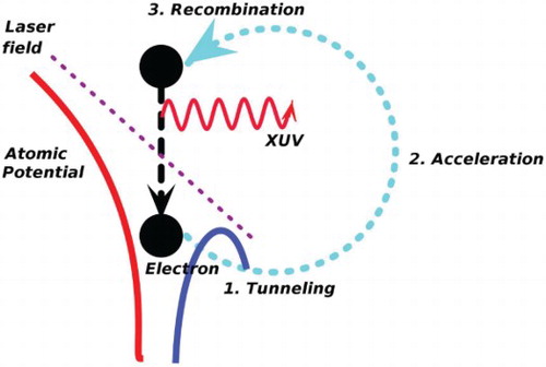
High-harmonic generation (HHG), in which a fundamental strong laser field is converted into harmonics of very high orders, is an avenue to generate coherent attosecond light pulses in the spectral range from extreme-ultraviolet (XUV) to the soft X-ray regions [15]. HHG process is by nature highly non-linear, and its spectrum has a distinctive shape; a plateau, where the intensity of the emitted radiation remains nearly constant up to many orders, and then an abrupt cutoff, beyond which practically no harmonics are observed [16]. These features can be intuitively explained by the semi-classical three-step model [17,18]; (i) an electron escapes to the continuum at the nuclear position with zero kinetic energy through tunnel ionisation, (ii) it moves classically and is driven back toward the parent ion by the laser field, and (iii) when the electron comes back to the parent ion and possibly recombines with it, a harmonic photon whose energy is the sum of the electron kinetic energy and the ionisation potential $I_p$ is emitted. Then, the cutoff energy $E_c$ is given by $E_c=I_p+3.17U_p$, where $U_p=E_0^2/4{\omega }_0^2$ denotes the ponderomotive energy ($E_0$: laser electric field strength, ${\omega }_0$: carrier frequency).

The time-dependent Schrödinger equation (TDSE) provides the rigorous theoretical description of the laser-induced multielectron dynamics. However, direct real-space solutions of the TDSE beyond two-electron systems remains a major challenge [19–28]. As a consequence, the single-active-electron (SAE) approximation [29,30] is widely used, in which only the outermost electron is explicitly treated. Laser-induced multielectron dynamics is, however, beyond the reach of this approximation.

One of the most advanced methods to describe the multielectron dynamics is the multiconfiguration time-dependent Hartree-Fock (MCTDHF) method [31–36] and more generally the time-dependent multiconfiguration self-consistent-field (TD-MCSCF) method. In TD-MCSCF, the electronic wavefunction is given by the configuration-interaction (CI) expansion, and both CI coefficients and spin-orbital functions constituting the Slater determinants are propagated in time.

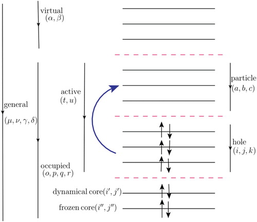
The applicability of the full CI-based MCTDHF method is significantly broadened by the time-dependent complete-active-space self-consistent-field (TD-CASSCF) method [37], which introduces the frozen-core, dynamical-core, and active orbital subspaces as illustrated in Figure 1. More approximate, and thus computationally more efficient methods [38–41] have been developed by relying on a truncated CI expansion within the active orbital space, compromising the size extensivity condition.

Figure 1. The orbital sub-spacing for a spin-restricted case. The horizontal lines represent spatial orbitals, divided into frozen-core, dynamical core, and active. The active orbital space is further split into the hole and particle subspaces those occupied and virtual with respect to the Hartree-Fock determinant. The up and down arrows represent electrons.

To restore the size-extensivity, the choice of the coupled-cluster expansion [42–44] within the time-dependent active orbitals is a worthy one. This idea was first realised by the orbital-adapted time-dependent coupled-cluster (OATDCC) method [45], which is based on the complex analytic action functional using the biorthonormal orbitals. We have also developed time-dependent optimised coupled-cluster (TD-OCC) method [46], based on the real action functional using time-dependent orthonormal orbitals.

Recently, to further extend the applicability to heavier atoms and larger molecules interacting with intense laser fields, we have implemented approximate methods within the TD-OCC framework without losing the size-extensivity criteria [47,48]. In Ref. [47], we introduced a method designated as TD-OCEPA0, which is based on the simplest version of the coupled-electron pair approximation [49]. We have also implemented an approximate method in the TD-OCC framework, based on the many-body perturbation expansion of the coupled-cluster effective Hamiltonian [48]. This method, designated as time-dependent orbital-optimised second-order many-body perturbation method (TD-OMP2), is a time-dependent extension of the orbital-optimised MP2 method developed by Bozkaya et al. [49] for the stationary electronic structure calculations. It is size-extensive, gauge-invariant, and has a lower scaling of the computational cost [$O(N^5)$ where N is the number of active orbitals] than the TD-OCC method with double excitations (TD-OCCD) having a scaling of $O(N^6)$. For both the TD-OMP2 and TD-OCEPA0 [47,48], one need not solve for de-excitation amplitudes since they are the complex conjugate of the excitation amplitudes, which further leads to a significant reduction in the computational cost.

Furthermore, in the present work, we report the implementation of the so-called CC2 method [50] within the active space in the time-dependent framework (TD-CC2). The CC2 method is also a second-order approximation to the coupled-cluster singles and doubles (CCSD) model. In this method, the doubles equation is approximated to provide the first-order corrections to the wavefunction, and the singles equation is kept the same as in the CCSD approximation. It scales $N^5$ and produces ground state comparable to the MP2 method. The equations of motions (EOMs) are derived based on the real-action formulation with orthonormal orbital functions, following our earlier work [46]. We have omitted hole-particle rotations in our implementation while retaining the single amplitudes [51]. The major drawback of the TD-CC2 method is the lack of gauge invariance, as numerically shown in this work.

There are numerous experiments performed on the noble gas atoms and their mixtures [52–57]. Harmonics of higher than 300 orders have been obtained. The TDDFT [58] is an attractive choice to study strong-field phenomena for larger chemical systems [59]. Shih-I Chu et al. [60] developed the self-interaction-free time-dependent density-functional theory (TDDFT) and extensively studied laser-driven dynamics in noble gas atoms [61], and also in heteronuclear diatomics [62]. However, their method [60] is not free from the general drawbacks of the DFT. The TD-OMP2 is a choice in the wavefunction based methods to reach out to larger chemical systems studying of strong-field dynamics with affordable scaling.

In this article, we apply the TD-OMP2 method to the study of laser-induced dynamics in Ne atom. Ne is having the highest ionisation potential value among the noble gas atoms (except for the He, for which anyway it is possible to have an exact solution of the TDSE [63–65]), and 2s and 2p orbitals are well separated from each other. These make Ne as an interesting candidate to deal with as a test case. It is also true that highly accurate results can be produced by the method like TD-CASSCF to have a better understanding of the capability of the newly implemented approximate methods before moving to larger chemical systems.

First, we seek for the most suitable active space configuration and the maximum angular momentum to expand the time-dependent orbitals for the study with the highest employed intensity by performing a series of calculations. Then, we compare the TD-OMP2 results with those of time-dependent Hartree-Fock (TDHF) and the TD-CASSCF for the highest employed intensity. Further, we report the results of time-dependent dipole-moment calculated using the TD-CC2 method and compare it with other methods and demonstrate that the property evaluated using this method is not gauge-invariant. We also report a comparison of the computational timing between the TD-OMP2 and TD-CC2 methods. The manuscript is organised as follows. A concise description of the TD-OMP2 and TD-CC2 method is presented in Section 2. Section 3 reports and discusses the numerical results. Finally, concluding remarks are given in Section 4. We use Hartree atomic units unless stated otherwise, and Einstein convention is implied for summation over orbital indices.

2. Method

We consider a system with N electrons governed by the following time-dependent Hamiltonian, (1) $H(t)=\sum _{i=1}^{N}h({\mathit{r}}_i,{\mathit{p}}_i,t)+\sum _{i=1}^{N-1}\sum _{j=2}^N\frac{1}{|{\mathit{r}}_i-{\mathit{r}}_j|},$(1) where ${\mathit{r}}_i$ and ${\mathit{p}}_i$ are the position and canonical momentum of an electron i. The corresponding second quantised Hamiltonian reads (2) $\hat{H}=h_{\nu }^{\mu }{\hat{c}}_{\mu }^{†}{\hat{c}}_{\nu }+\frac{1}{2}{u}_{\nu \lambda }^{\mu \gamma }{\hat{c}}_{\mu }^{†}{\hat{c}}_{\gamma }^{†}{\hat{c}}_{\lambda }{\hat{c}}_{\nu },$(2) where ${\hat{c}}_{\mu }^{†}$ (${\hat{c}}_{\mu }$) is a creation (annihilation) operator for the complete, orthonormal set of spin-orbitals $\{{\psi }_{\mu }(t)\}$, which are explicitly time-dependent, and (3) $\begin{array}{rl}{h}_{\nu }^{\mu }& =\int \mathrm{d}{x}_1{\psi }_{\mu }^{\ast }(x_1)h({\mathit{r}}_1,{\mathit{p}}_1){\psi }_{\nu }(x_1),\end{array}$(3) (4) $\begin{array}{rl}{u}_{\nu \lambda }^{\mu \gamma }& =\iint \mathrm{d}{x}_1\mathrm{d}{x}_2\frac{{\psi }_{\mu }^{\ast }(x_1){\psi }_{\gamma }^{\ast }(x_2){\psi }_{\nu }(x_1){\psi }_{\lambda }(x_2)}{|{\mathit{r}}_1-{\mathit{r}}_2|},\end{array}$(4) where $x_i=({\mathit{r}}_i,{\sigma }_i)$ is a composite spatial-spin coordinate. Hereafter we refer to spin-orbitals simply as orbitals, and use orbital indices $i,j,k\cdots$ to denote orbitals in the hole space which are occupied in a reference determinant Φ, and $a,b,c,\dots$ for those in the particle space which are unoccupied in the reference and accommodate excited electrons. We use $p,q,r,\dots$ for general active orbitals (union of hole and particle). It should be noted that, as an orbital-optimised theory, the number of active orbitals is less than the number of the full set of the orbitals $\{{\psi }_{\mu }\}$ in general [37,41,46–48].

2.1. Review of TD-OMP2 method

The ground-state MP2 method can be viewed as an approximation to the CCD method considering only those terms which give first-order contributions to the wavefunction with respect to the fluctuation potential [66]. To construct the TD-OMP2 method as a time-dependent, orbital-optimised counterpart of the MP2 method, we begin with the time-dependent CCD Lagrangian, and retain only those terms giving up to second-order contributions to the Lagrangian [48], which reads (5) $\begin{array}{rl}L& =L_0-i{\lambda }_{ab}^{ij}{\dot{\tau }}_{ij}^{ab}+⟨\mathrm{\Phi }|{\hat{\mathrm{\Lambda }}}_2(\hat{H}-i\hat{X})|\mathrm{\Phi }⟩\\ & +⟨\mathrm{\Phi }|[\hat{H}-i\hat{X},{\hat{T}}_2]|\mathrm{\Phi }⟩+⟨\mathrm{\Phi }|{\hat{\mathrm{\Lambda }}}_2[\hat{f}-i\hat{X},{\hat{T}}_2]|\mathrm{\Phi }⟩,\end{array}$(5) where $L_0=⟨\mathrm{\Phi }|(\hat{H}-i\mathrm{\partial }/\mathrm{\partial }t)|\mathrm{\Phi }⟩$, $\hat{f}=f_{\nu }^{\mu }{\hat{c}}_{\mu }^{†}{\hat{c}}_{\nu }$, $\hat{X}=X_{\nu }^{\mu }{\hat{c}}_{\mu }^{†}{\hat{c}}_{\nu }$, $f_{\nu }^{\mu }\equiv h_{\nu }^{\mu }+v_{\nu j}^{\mu j}$, $X_{\mu }^{\nu }=⟨{\psi }_{\nu }|{\dot{\psi }}_{\mu }⟩$, $v_{qs}^{pr}\equiv u_{qs}^{pr}-u_{sq}^{pr}$, $\widehat{T_2}={\tau }_{ij}^{ab}{\hat{c}}_a^{†}{\hat{c}}_b^{†}{\hat{c}}_j{\hat{c}}_i$, and ${\hat{\mathrm{\Lambda }}}_2={\lambda }_{ab}^{ij}{\hat{c}}_i^{†}{\hat{c}}_j^{†}{\hat{c}}_b{\hat{c}}_a$. Then the action functional (6) $S={\int }_{t_0}^{t_1}L(t)\mathrm{d}t$(6) is required to be stationary, $\delta S=0$, with respect to the variation of the amplitudes $\{{\tau }_{ij}^{ab}\}$, $\{{\lambda }_{ab}^{ij}\}$ and orthonormality-conserving variation of orbitals [48]. The resultant EOM for amplitudes reads (7) $i{\dot{\tau }}_{ij}^{ab}=v_{ij}^{ab}-p(ij)f_j^k{\tau }_{ik}^{ab}+p(ab)f_c^a{\tau }_{ij}^{cb},{\lambda }_{ab}^{ij}={\tau }_{ij}^{ab\ast }$(7) where $p(ij)$ and $p(ab)$ are the cyclic permutation operator. We have also arbitrarily chosen one of the orbital gauges $⟨{\psi }_i|{\dot{\psi }}_j⟩=⟨{\psi }_a|{\dot{\psi }}_b⟩=0$, using the invariance of the total wavefunction with respect to the unitary transformation within the hole and particle spaces separately to simplify the equations of motion.

The EOMs for orbitals are given by (8) $\begin{array}{rl}& i|\dot{{\psi }_p}⟩=(1-\hat{P}){\hat{F}}_p|{\psi }_p⟩+|{\psi }_q⟩X_p^q,\end{array}$(8) (9) $\begin{array}{rl}& i\{({\delta }_b^a{\rho }_i^j-{\rho }_b^a{\delta }_i^j)X_j^b\}=F_j^a{\rho }_i^j-{\rho }_b^a{F}_b^{i\ast }\end{array}$(9) (10) $\begin{array}{rl}& {\hat{F}}_p|{\psi }_p⟩=\hat{h}|{\psi }_p⟩+{\hat{W}}_s^r|{\psi }_q⟩{\rho }_{or}^{qs}{({\rho }^{-1})}_p^o,\end{array}$(10) (11) $\begin{array}{rl}& W_s^r({\mathit{x}}_1)=\int \mathrm{d}{\mathit{x}}_2\frac{{\psi }_r^{\ast }({\mathit{x}}_2){\psi }_s({\mathit{x}}_2)}{|{\mathit{r}}_1-{\mathit{r}}_2|},\end{array}$(11) where $\hat{P}=\sum _p|{\psi }_p⟩⟨{\psi }_p|$, $F_q^p=⟨{\varphi }_p|F_q|{\varphi }_q⟩$, and ${\rho }_q^p$ and ${\rho }_{qs}^{pr}$ are the one- and two-body reduced density matrices given by (12) $\begin{array}{rl}{\rho }_p^q& ={\gamma }_p^q+{\delta }_j^q{\delta }_p^j,{\rho }_{pr}^{qs}={\mathrm{\Gamma }}_{pr}^{qs}+{\gamma }_p^q{\delta }_j^s{\delta }_r^j+{\gamma }_r^s{\delta }_j^q{\delta }_p^j-{\gamma }_r^q{\delta }_j^s{\delta }_p^j\\ & -{\gamma }_p^s{\delta }_j^q{\delta }_r^j+{\delta }_j^q{\delta }_p^j{\delta }_k^s{\delta }_r^k-{\delta }_j^s{\delta }_p^j{\delta }_k^q{\delta }_r^k,\end{array}$(12) with non-zero elements of ${\gamma }_p^q$ and ${\mathrm{\Gamma }}_{pr}^{qs}$ being (13) $\begin{array}{rl}{\gamma }_j^i& =-\frac{1}{2}{{\tau }_{ki}^{cb}}^{†}{\tau }_{kj}^{cb},{\gamma }_a^b=\frac{1}{2}{{\tau }_{kl}^{ca}}^{†}{\tau }_{kl}^{cb},{\mathrm{\Gamma }}_{ij}^{ab}={\tau }_{ij}^{ab},\\ & {\mathrm{\Gamma }}_{ab}^{ij}={{\tau }_{ij}^{ab}}^{†}.\end{array}$(13)

2.2. TD-CC2 method

The stationary CC2 method can be viewed as an approximation to the CCSD method considering only those terms which give first-order contributions to the wavefunction with respect to the fluctuation potential [50]. To construct the TD-CC2 method as a time-dependent counterpart of the CC2 method, we shall begin with the time-dependent CCSD Lagrangian, and retain only those terms giving up to second-order contributions to the wavefunction, which reads (14) $\begin{array}{rl}L& =L_0-i{\lambda }_a^i{\dot{\tau }}_i^a-i{\lambda }_{ab}^{ij}{\dot{\tau }}_{ij}^{ab}+⟨\mathrm{\Phi }|({\hat{\mathrm{\Lambda }}}_1+{\hat{\mathrm{\Lambda }}}_2)(\overline{H}-i\overline{X})|\mathrm{\Phi }⟩\\ & +⟨\mathrm{\Phi }|[\overline{H}-i\overline{X},{\hat{T}}_2]|\mathrm{\Phi }⟩+⟨\mathrm{\Phi }|{\hat{\mathrm{\Lambda }}}_1[\overline{H}-i\overline{X},{\hat{T}}_2]|\mathrm{\Phi }⟩\\ & +⟨\mathrm{\Phi }|{\hat{\mathrm{\Lambda }}}_2[\overline{f}-i\overline{X},{\hat{T}}_2]|\mathrm{\Phi }⟩,\end{array}$(14) where $\overline{O}\equiv e^{-{\hat{T}}_1}\hat{O}{e}^{{\hat{T}}_1}$, ${\hat{T}}_1={\tau }_i^a{\hat{c}}_a^{†}{\hat{c}}_i$, and ${\hat{\mathrm{\Lambda }}}_1={\lambda }_a^i{\hat{c}}_i^{†}{\hat{c}}_a$. It should be noticed that the singles amplitudes ${\tau }_i^a,{\lambda }_a^i$ are treated as a zeroth-order quantity. Then, following the real-valued action formulation as described in the previous section, we derive the amplitude EOMs as (15) $\begin{array}{rl}i{\dot{\tau }}_i^a& =⟨{\mathrm{\Phi }}_i^a|\overline{H}-i\overline{X}+[\overline{H}-i\overline{X},{\hat{T}}_2]|\mathrm{\Phi }⟩,\end{array}$(15) (16) $\begin{array}{rl}i{\dot{\tau }}_{ij}^{ab}& =⟨{\mathrm{\Phi }}_{ij}^{ab}|\overline{H}-i\overline{X}+[\overline{f}-i\overline{X},{\hat{T}}_2]|\mathrm{\Phi }⟩,\end{array}$(16) (17) $\begin{array}{rl}-i{\dot{\lambda }}_a^i& =⟨\mathrm{\Phi }|(1+{\hat{\mathrm{\Lambda }}}_1)[\hat{H}-i\hat{X}+[\hat{H}-i\hat{X},{\hat{T}}_2],{\hat{E}}_i^a]|\mathrm{\Phi }⟩\\ & +⟨\mathrm{\Phi }|{\hat{\mathrm{\Lambda }}}_2[\hat{H}-i\hat{X}+[\hat{f}-i\hat{X},{\hat{T}}_2],{\hat{E}}_i^a]|\mathrm{\Phi }⟩,\end{array}$(17) (18) $\begin{array}{rl}-i{\dot{\lambda }}_{ab}^{ij}& =⟨\mathrm{\Phi }|(1+{\hat{\mathrm{\Lambda }}}_1)[\overline{H}-i\overline{X},{\hat{E}}_{ij}^{ab}]|\mathrm{\Phi }⟩\\ & +⟨\mathrm{\Phi }|{\hat{\mathrm{\Lambda }}}_2[\overline{f}-i\overline{X},{\hat{E}}_{ij}^{ab}]|\mathrm{\Phi }⟩,\end{array}$(18) Expanding right-hand sides of the Equations (15(15) $\begin{array}{rl}i{\dot{\tau }}_i^a& =⟨{\mathrm{\Phi }}_i^a|\overline{H}-i\overline{X}+[\overline{H}-i\overline{X},{\hat{T}}_2]|\mathrm{\Phi }⟩,\end{array}$(15) )–(18(18) $\begin{array}{rl}-i{\dot{\lambda }}_{ab}^{ij}& =⟨\mathrm{\Phi }|(1+{\hat{\mathrm{\Lambda }}}_1)[\overline{H}-i\overline{X},{\hat{E}}_{ij}^{ab}]|\mathrm{\Phi }⟩\\ & +⟨\mathrm{\Phi }|{\hat{\mathrm{\Lambda }}}_2[\overline{f}-i\overline{X},{\hat{E}}_{ij}^{ab}]|\mathrm{\Phi }⟩,\end{array}$(18) ) in terms of one-body and two-body matrix elements obtain programmable algebraic expressions, Equations (A1(A1) $\begin{array}{rl}i{\dot{\tau }}_i^a& =f_i^a+f_c^k{\tau }_{ki}^{ca}+0.5v_{cd}^{ak}{\tau }_{ik}^{cd}-0.5v_{ic}^{kl}{\tau }_{kl}^{ac}\\ & +f_c^a{\tau }_i^c-f_i^k{\tau }_k^a+v_{ic}^{ak}{\tau }_k^c\\ & +v_{cd}^{kl}{\tau }_{kl}^{ad}{\tau }_i^c-0.5v_{cd}^{kl}{\tau }_{il}^{cd}{\tau }_k^a+v_{cd}^{kl}{\tau }_l^d{\tau }_{ki}^{ca}\\ & -f_c^k{\tau }_i^c{\tau }_k^a+v_{cd}^{ak}{\tau }_k^d{\tau }_i^c\\ & -v_{ic}^{kl}{\tau }_l^c{\tau }_k^a-v_{cd}^{kl}{\tau }_l^d{\tau }_i^c{\tau }_k^a\end{array}$(A1) )–(A4(A4) $\begin{array}{rl}-i{\dot{\lambda }}_{ab}^{ij}& =v_{ab}^{ij}+p(ij|ab)f_a^i{\lambda }_b^j+p(ij|ab)v_{ac}^{ik}{\tau }_k^c{\lambda }_b^j+p(ij)v_{ab}^{ic}{\lambda }_c^j\\ & -p(ab)v_{ak}^{ij}{\lambda }_b^k-p(ij)v_{ab}^{ik}{\tau }_k^c{\lambda }_c^j-p(ab)v_{ac}^{ij}{\tau }_k^c{\lambda }_b^k\\ & +p(ab)f_a^c{\lambda }_{cb}^{ij}\\ & -p(ij)f_k^i{\lambda }_{ab}^{kj}-p(ij)f_c^i{\tau }_k^c{\lambda }_{ab}^{jk}-p(ab)f_a^k{\tau }_k^c{\lambda }_{cb}^{ij}\end{array}$(A4) ).

The EOMs for orbitals are derived as (19) $i|\dot{{\psi }_p}⟩=(1-\hat{P}){\hat{F}}_p|{\psi }_p⟩,$(19) which is formally identical to those for TD-OMP2, Equation (8(8) $\begin{array}{rl}& i|\dot{{\psi }_p}⟩=(1-\hat{P}){\hat{F}}_p|{\psi }_p⟩+|{\psi }_q⟩X_p^q,\end{array}$(8) ), except for the absence of the second term, where (i) again we arbitrarily chose $X_i^j=X_a^b=0$, and (ii) the hole-particle rotations are also fixed as $X_i^a=0$). We adopted the latter, because both real- and imaginary-time propagation encounters convergence difficulty due to similar roles played by ${\hat{T}}_1$ amplitudes and hole-particle rotations. (See [46,51] for the related discussions for the stationary problems.) The correlation contributions of the density matrices for the TD-CC2 method are given in Equations (A5(A5) $\begin{array}{rl}{\gamma }_a^i& ={\lambda }_a^i,{\gamma }_i^a={\tau }_i^a+{\lambda }_b^j{\tau }_{ij}^{ab}+{\lambda }_b^j{\tau }_i^b{\tau }_j^a-0.5{\lambda }_{cd}^{kl}{\tau }_{ki}^{cd}{\tau }_l^a\\ & -0.5{\lambda }_{cd}^{kl}{\tau }_{kl}^{ca}{\tau }_i^d\\ {\gamma }_j^i& ={\lambda }_a^i{\tau }_j^a-0.5{\lambda }_{cb}^{ki}{\tau }_{kj}^{cb},{\gamma }_b^a={\lambda }_b^i{\tau }_i^a+0.5{\lambda }_{cb}^{kl}{\tau }_{kl}^{ca}\end{array}$(A5) ) and (A6(A6) $\begin{array}{rl}& {\mathrm{\Gamma }}_{cd}^{ab}={\lambda }_{cd}^{ij}{\tau }_i^a{\tau }_j^b,{\mathrm{\Gamma }}_{kl}^{ij}={\lambda }_{cd}^{ij}{\tau }_k^c{\tau }_l^d,{\mathrm{\Gamma }}_{ak}^{bc}={\lambda }_a^l{\tau }_{lk}^{bc}\\ & +p(bc){\lambda }_a^l{\tau }_l^b{\tau }_k^c,{\mathrm{\Gamma }}_{jk}^{ic}=-{\lambda }_b^i{\tau }_{jk}^{bc}-p(jk){\lambda }_b^i{\tau }_j^b{\tau }_k^c\\ & {\mathrm{\Gamma }}_{al}^{bc}=-{\lambda }_{ad}^{ij}{\tau }_i^a{\tau }_j^c{\tau }_l^d,{\mathrm{\Gamma }}_{jl}^{ic}={\lambda }_{ad}^{ik}{\tau }_j^a{\tau }_k^c{\tau }_l^d,{\mathrm{\Gamma }}_{ca}^{jb}={\lambda }_{ca}^{ji}{\tau }_i^b,\\ & {\mathrm{\Gamma }}_{ci}^{ka}=-{\lambda }_{ac}^{ik}{\tau }_i^a\\ & {\mathrm{\Gamma }}_{ij}^{ab}={\tau }_{ij}^{ab}+0.5p(ij|ab){\tau }_i^a{\tau }_j^b+p(ij|ab){\lambda }_c^k{\tau }_{ki}^{ca}{\tau }_j^b\\ & -p(ij){\lambda }_c^k{\tau }_i^c{\tau }_{kj}^{ab}-p(ab){\lambda }_c^k{\tau }_k^a{\tau }_{ij}^{cb}\\ & -p(ij|ab){\lambda }_c^k{\tau }_k^a{\tau }_i^c{\tau }_j^b+{\lambda }_{cd}^{kl}{\tau }_i^c{\tau }_j^d{\tau }_k^a{\tau }_l^b\\ & {\mathrm{\Gamma }}_{aj}^{ib}={\lambda }_a^i{\tau }_j^b-{\lambda }_{ac}^{ik}{\tau }_k^b{\tau }_j^c,{\mathrm{\Gamma }}_{ab}^{ij}={\lambda }_{ab}^{ij}\end{array}$(A6) ).

In summary, TD-CC2 method differs from the TD-OMP2 method in that it includes the singles amplitudes and ignores the hole-particle rotations. While the former treatment (CC2) is usually preferred in the stationary theory, we consider that the latter approach (TD-OMP2) is advantageous in the time-dependent problems, since the omission of the hole-particle rotation results in the loss of gauge-invariance of the TD-CC2 method, as numerically demonstrated in the next section.

3. Results and discussion: application to electron dynamics in Ne

In this section, we report and discuss the application of our numerical implementation of the TD-OMP2 method to laser-driven electron dynamics in Ne atom. Within the dipole approximation in the velocity gauge, the one-electron Hamiltonian is given by (20) $h(\mathit{r},\mathit{p})=\frac{1}{2}|{\mathit{p}}^2|-\frac{Z}{|\mathit{r}|}+A(t)p_z$(20) where Z = 10 is the atomic number, $A(t)=-{\int }^{t}E(t^{\mathrm{\prime }})\mathrm{d}{t}^{\mathrm{\prime }}$ is the vector potential, with $E(t)$ being the laser electric field linearly polarised along z axis, given as (21) $E(t)=E_0\sin ({\omega }_{0}t){\sin }^2\left(\pi \frac{t}{\tau }\right),0\le t\le \tau ,$(21) with a foot-to-foot pulse duration τ (3T), a peak intensity $I_0=E_0^2$, period $T=2\pi /{\omega }_0$, and a wavelength of $\lambda =2\pi /{\omega }_0$.

In our implementation, the time-dependent orbitals are expanded with spherical-FEDVR basis functions, (22) ${\chi }_{klm}(r,\theta ,\psi )=\frac{1}{r}{f}_k(r)Y_{lm}(\theta ,\varphi )$(22) where, $Y_{lm}$ and $f_k(r)$ are spherical harmonics and the normalised radial-FEDVR basis function [67,68], respectively. The spherical harmonics expansion is continued up to the maximum angular momentum of $L_{\max }$, and the radial FEDVR basis supports the range of radial coordinate $0\le r\le R_{\max }$, with an appropriate absorbing boundary condition. The details of the implementation can be found in [69,70]. We have used fourth-order exponential Runge-Kutta integrator [71] to propagate equations of motions with 10,000 time-steps per optical cycle. The simulations are run for further 3000 time steps after the end of the pulse. We have used a regularisation while inverting the one-body reduced density matrix in Equation (10(10) $\begin{array}{rl}& {\hat{F}}_p|{\psi }_p⟩=\hat{h}|{\psi }_p⟩+{\hat{W}}_s^r|{\psi }_q⟩{\rho }_{or}^{qs}{({\rho }^{-1})}_p^o,\end{array}$(10) ). Details of the functional form of the regulariser can be found in Ref. [41].

First, we seek for the optimum orbital space for our study, by changing the numbers ($n_{\mathrm{fc}}$, $n_{\mathrm{dc}}$, $n_{\mathrm{act}}$), where $n_{\mathrm{fc}}$ is the number of frozen-core orbitals which are forced to be doubly occupied and fixed in time, $n_{\mathrm{dc}}$ is the number of dynamical-core orbitals $n_{\mathrm{dc}}$ which are forced to be doubly occupied but propagated in time, and $n_{\mathrm{act}}$ is the number of active orbitals among which the active electrons are correlated. We have chosen a laser field having a wavelength of 800 nm with an intensity of $1\times {10}^{15}\mathrm{W}/{\mathrm{cm}}^2$. We have used a simulation box size of $R_{\max }=300$ with ${\cos }^{1/4}$ mask function switched on at 240 with $L_{\max }=63$. 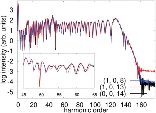We have performed a series of calculations starting from 8-active electrons in 8-active orbitals and gradually increased to 10-active electrons in 14-active orbitals (Figure 2). We found that the HHG spectrum computed with the configuration $(1,0,13)$ meet a virtually perfect agreement with the one computed with the configuration $(0,0,14)$. Therefore, we have chosen the active-space configuration $(1,0,13)$ in all the following simulations.

Figure 2. HHG spectra of Ne exposed to a laser pulse with a wavelength of 800 nm and an intensity of $1\times {10}^{15}\mathrm{W}/{\mathrm{cm}}^2$. Results of the TD-OMP2 method with different numbers of orbital configuration (m, n, o) and maximum angular momentum $L_{\max }=63$.

Next, in Figure 3, we report the convergence pattern of the HHG spectra with respect to the maximum angular momentum $L_{\max }$ to expand the orbitals. A series of simulations are performed for $51\le L_{\max }\le 75$ with an intensity of $1\times {10}^{15}\mathrm{W}/{\mathrm{cm}}^2$ and a wavelength of 800 nm, with an orbital configuration $(1,0,13)$. As seen in Figure 3, the results steadily tend to converge to the result obtained employing the highest angular momentum $L_{\max }=75$, and especially, the spectrum with $L_{\max }=63$ meets the perfect agreement with $L_{\max }=75$ within the graphical resolution. Therefore, we have chosen $L_{\max }=63$ as the optimum (necessary-and-sufficient) value for the $L_{\max }$ in all the following simulations with an 800 nm wavelength laser pulse.

Figure 3. HHG spectra of Ne exposed to a laser pulse with a wavelength of 800 nm and an intensity of $1\times {10}^{15}\mathrm{W}/{\mathrm{cm}}^2$. Results of the TD-OMP2 method obtained with different maximum angular momentum $L_{\max }$ with the orbital configuration $(1,0,13)$.

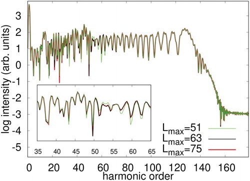
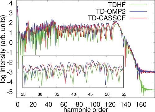
Figure 4 shows comparison of the HHG spectra for the applied laser intensities $5\times {10}^{14}\mathrm{W}/{\mathrm{cm}}^2$, $8\times {10}^{14}\mathrm{W}/{\mathrm{cm}}^2$, and $1\times {10}^{15}\mathrm{W}/{\mathrm{cm}}^2$ with a constant wavelength of 800 nm. One can see the dramatic extension of the cut-off energy with an increase in the applied laser intensity. One also observes an increase of the harmonic yield by nearly one order of magnitude in comparison of the lowest and medium intensity cases, and the saturation of the intensity in comparison of the medium and highest intensity cases. It is important to note that these results are obtained with a well-calibrated conditions described above, and therefore, reliable as converged result within the TD-OMP2 approximation. In Figure 5, we have compared the results from the TD-OMP2 simulations with the fully correlated TD-CASSCF method, and the uncorrelated TDHF method.

Figure 4. HHG spectra of Ne exposed to a laser pulse having a wavelength of 800 nm and varying intensities of $5\times {10}^{14}\mathrm{W}/{\mathrm{cm}}^2$, $8\times {10}^{14}\mathrm{W}/{\mathrm{cm}}^2$, and $1\times {10}^{15}\mathrm{W}/{\mathrm{cm}}^2$, obtained with the TD-OMP2 method with an orbital configuration $(1,0,13)$ and maximum angular momentum $L_{\max }=63$.

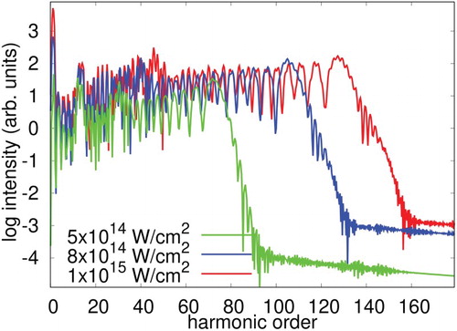
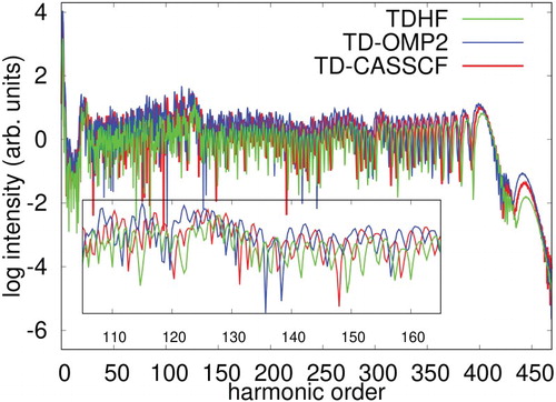
Figure 5. HHG spectra of Ne exposed to laser pulse with a wavelength of 800 nm and an intensity $1\times {10}^{15}\mathrm{W}/{\mathrm{cm}}^2$, Comparison of TD-OMP2 method with TD-CASSCF, and TDHF methods. Maximum angular momentum $L_{\max }=63$ and $(1,0,13)$ active space configuration for the correlation methods has been used.

Now we move to a longer wavelength case with $\lambda =1200\mathrm{nm}$, which is a relatively difficult simulation condition, and serves as a robust test for the newly implemented TD-OMP2 method. We follow the same procedure as made above for the case with $\lambda =800\mathrm{nm}$. First we test various $L_{\max }$ for the highest-applied intensity of $1\times {10}^{15}\mathrm{W}/{\mathrm{cm}}^2$. We used TDHF method for the calibration here, and obtained $L_{\max }=100$ as the optimum (necessary-and-sufficient) value for the maximum angular momentum as confirmed in Figure 6. We, therefore, use $L_{\max }=100$ for the following simulations to see the intensity dependence of the HHG spectra (Figure 7) obtained with TD-OMP2, and the comparison of TDHF, TD-OMP2, and TD-CASSCF results (Figure 8). We could derive essentially the same conclusion from these application as that for $\lambda =800\mathrm{nm}$. The TDHF severely underestimate the harmonic intensity for the longer wavelength. On the other hand, the agreement between the TD-OMP2 and TD-CASSCF spectra is better for $\lambda =1200\mathrm{nm}$ than for $\lambda =800\mathrm{nm}$. Importantly, the agreement between the TD-OMP2 and TD-CASSCF results here indicates the convergence of the result with respect to the level of inclusion of the correlation effect, with sufficiently large $L_{\max }$, i.e. at the basis set limit. In general, TDHF tends to underestimate, and TD-OMP2 overestimates taking TD-CASSCF as the benchmark. However, the extent of deviation for both TDHF and TD-OMP2 is less for the longer wavelength.

Figure 6. HHG spectra of Ne exposed to a laser pulse with a wavelength of 1200 nm and an intensity of $1\times {10}^{15}\mathrm{W}/{\mathrm{cm}}^2$. Results of the TDHF method obtained with different maximum angular momentum $L_{\max }$.

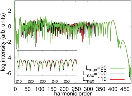
Figure 7. HHG spectra of Ne exposed to laser pulse with a wavelength of 1200 nm and varying intensities of $5\times {10}^{14}\mathrm{W}/{\mathrm{cm}}^2$, $8\times {10}^{14}\mathrm{W}/{\mathrm{cm}}^2$, and $1\times {10}^{15}\mathrm{W}/{\mathrm{cm}}^2$, obtained with TD-OMP2 method with the orbital configuration $(1,0,13)$ and the maximum angular momentum $L_{\max }=100$.

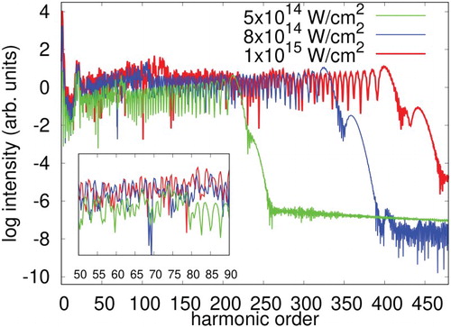
Figure 8. HHG spectra of Ne exposed to laser pulse with a wavelength of 1200 nm having intensity of $1\times {10}^{15}\mathrm{W}/{\mathrm{cm}}^2$, Comparison of TD-OMP2 method with TD-CASSCF, and TDHF method. Maximum angular momentum $L_{\max }=100$ and $(1,0,13)$ active space configuration for the correlation methods has been used.

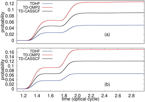
To establish our findings further, we report the time-evolution of dipole moment and single ionisation probability at an intensity of $1\times {10}^{15}\mathrm{W}/{\mathrm{cm}}^2$ having a wavelength of (a) 800 nm, and (b) 1200 nm in Figures 9 and 10, respectively. The dipole moment is calculated as a trace $⟨{\psi }_p|\hat{z}|{\psi }_q⟩{\rho }_p^q$, and the single ionisation probability is evaluated as the probability of finding an electron outside a sphere of radius 20 a.u. We have used the same optimised simulation condition for each wavelength, as reported earlier. In general, TDHF tends to underestimate, whereas TD-OMP2 overestimates in comparison to the TD-CASSCF; the deviation is more for TDHF, however. Such a convergence pattern for these methods is often encountered in the ground state calculations also. The difference from the TD-CASSCF for both TDHF and TD-OMP2 reduces for the longer wavelength (Figure 9(b)), however, for the ionisation probability, the difference between these methods remains nearly constant shown in Figure 10(b). The role of electron correlation is less for the longer wavelength, as it is the outer valence electrons, which are driven by the incident laser.

Figure 9. Time evolution of the dipole moment of Ne irradiated by a laser pulse of a wavelength of (a) 800 nm, (b) 1200 nm at an intensity of $1\times {10}^{15}\mathrm{W}/{\mathrm{cm}}^2$, calculated with TDHF, TD-OMP2 and TD-CASSCF methods.

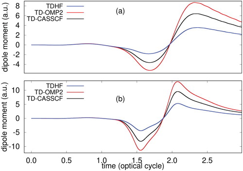
Figure 10. Time evolution of single ionisation probability of Ne irradiated by a laser pulse of a wavelength of (a) 800 nm, (b) 1200 nm at an intensity of $1\times {10}^{15}\mathrm{W}/{\mathrm{cm}}^2$, calculated with TDHF, TD-OMP2 and TD-CASSCF methods.

In Figure 11, we have compared time-evolution of dipole-moment of Ne with all these methods at an intensity of $5\times {10}^{13}\mathrm{W}/{\mathrm{cm}}^2$ at a wavelength of 800 nm. In these simulations, we also correlated 8 electrons in 13 active orbitals, and laser electric field taken in the velocity gauge. We are unsuccessful in obtaining a stable convergence for the TD-OCC2 method using laser intensities employed for the TD-OMP2 simulations. The ionisation potential of Ne is high, and the employed intensity is low enough to have sufficient ionisation. Therefore, the role of electron correlation is not that relevant in this particular case, and all the methods predict nearly identical time-dependent dipole moment. In Figure 12, we have reported HHG spectra. Except for the TD-CC2 method, all the other methods produce similar spectra. It overestimates high-harmonic intensity from all other methods. The outcome makes a clear case for the need of a low-scaling orbital-optimised theory. In Figure 13, we compare HHG spectra taking the laser-electric field in the length gauge with the result obtained with the velocity gauge treatment using the TD-OMP2 (Figure a) and TD-CC2 (Figure b) method. 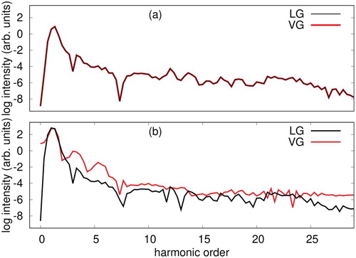We have used identical simulations conditions ($l_{\max },r_{\max }$, active space configuration) for these length gauge simulations as used for all other velocity gauge treatment using 800 nm wavelength laser. The outcome suggests that the TD-CC2 method does not provide a gauge-invariant description of properties of interest, whereas TD-OMP2 does, which make TD-OMP2 a superior choice for the study of strong-field dynamics.

Figure 11. Time evolution of the dipole moment of Ne irradiated by a laser pulse of a wavelength of 800 nm at an intensity of $5\times {10}^{13}\mathrm{W}/{\mathrm{cm}}^2$, calculated with TDHF, TD-OMP2, TD-CC2 and TD-CASSCF methods.

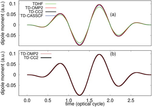
Figure 12. HHG spectra of Ne irradiated by a laser pulse of a wavelength of 800 nm at an intensity of $5\times {10}^{13}\mathrm{W}/{\mathrm{cm}}^2$, calculated with TDHF, TD-OMP2, TD-CC2 and TD-CASSCF methods.

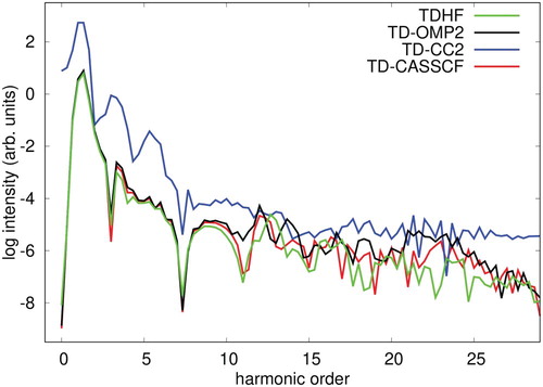
Figure 13. HHG spectra of Ne in the length gauge (LG) and velocity gauge (VG) irradiated by a laser pulse of a wavelength of 800 nm at an intensity of $5\times {10}^{13}\mathrm{W}/{\mathrm{cm}}^2$, calculated with (a) TD-OMP2, and (b) TD-CC2 method.

In the TD-OMP2 method, the doubly excited determinants are approximately incorporated in the configuration space. Therefore, it takes into account at least a part of the electron correlation, which makes it overall a better performer in comparison to the TDHF, where the electron correlation is missing. The electron correlation is more important in the far part of the spectrum, where the intensity profile of the spectrum drops quickly for TDHF, or in other words, the difference with the TD-CASSCF is more for the TDHF than TD-OMP2.

In Table 1, we compare computational timing for 1000 time-step propagation in various parts of TD-CC2 and TD-OMP2 methods for the real-time simulations. Even though the overall computational scaling for both the methods is the same ($N^5$), the TD-OMP2 does not involve solutions of the $T_1$, ${\mathrm{\Lambda }}_1$, and the ${\mathrm{\Lambda }}_2$ amplitude equations. The ${\mathrm{\Lambda }}_2$ amplitudes are complex conjugate of the $T_2$ amplitudes due to the linear structure of the functional. The $T_2$ equation for the TD-CC2 method has many terms and involves multiple operator products. The time saving for the TD-OMP2 method comes from the evaluation of 2RDMs, which scales N${}^4$ and does not involve any operator products. On the other hand, it is $N^5$ for the TD-CC2 method.

Table 1. Comparison of the CPU time (in second) spent for the evaluation of the $T_1$, ${\mathrm{\Lambda }}_1$, $T_2$, ${\mathrm{\Lambda }}_2$ equation, 1RDM, and 2RDM for TD-CC2 and TD-OMP2 methods.

TD-CC2						TD-OMP2
T${}_1$	${\mathrm{\Lambda }}_1$	T${}_2$	${\mathrm{\Lambda }}_2$	1RDM	2RDM	T${}_1$	${\mathrm{\Lambda }}_1$	T${}_2$	${\mathrm{\Lambda }}_2$	1RDM	2RDM
1.31	10.47	8.59	2.47	2.48	17.46	–	–	0.71	–	1.06	0.67

Note: CPU time spent for the simulation of Ne atom for 1000 time steps ($0\le t\le 0.1T$) of a real-time simulation ($I_0=5\times {10}^{13}\mathrm{W}/{\mathrm{cm}}^2$ and $\lambda =800\mathrm{nm}$), using an Intel(R) Xeon(R) Gold 6230 CPU with 40 processors having a clock speed of 2.10 GHz.

4. Concluding remarks

In this article, we have applied the recently developed TD-OMP2 method to compute the HHG spectra of Ne atom as a case study to analyse the performance of the implemented method in demanding laser conditions. Further, we have implemented the TD-CC2 method, which is also an N${}^5$ scaling second-order approximation to the parent TD-CCSD method. The TD-CC2 method does not provide a gauge-invariant description of the properties of interest and is not stable with rigorous simulations conditions, often required while studying strong-field dynamics. On the contrary, TD-OMP2 is very stable, does not breakdown even with harsher simulation conditions, and it is gauge-invariant. Additionally, TD-OMP2 is computationally more favourable. All these make TD-OMP2 as a superior choice over the TD-CC2 method. While the performance of the TD-OMP2 method is moderate, it is remarkable that such highly nonlinear nonperturbative phenomena can be stably computed within the framework of time-dependent perturbation method, by virtue of the nonperturbative inclusion of the laser-electron interaction and time-dependent optimisation of orbitals. This will open a way to correlated time-dependent calculation for large chemical systems, for which the applications of multiconfiguration methods such as TD-CASSCF are challenging. The method will also be useful to study moderate size systems; calibrations of simulation conditions and extensive parameter surveys can be performed before stepping into simulations with more rigorous and therefore, more expensive method.

Acknowledgments

This research was supported in part by a Grant-in-Aid for Scientific Research (Grants No. 16H03881, No. 17K05070, No. 18H03891, and No. 19H00869) from the Ministry of Education, Culture, Sports, Science and Technology (MEXT) of Japan. This research was also partially supported by JST COI (Grant No. JPMJCE1313), JST CREST (Grant No. JPMJCR15N1), and by MEXT Quantum Leap Flagship Program (MEXT Q-LEAP) Grant Number JPMXS0118067246. This research was also partially supported by Startup funding of Graduate School of Engineering, The University of Tokyo.

Disclosure statement

No potential conflict of interest was reported by the authors.

Additional information

Funding

This research was supported in part by a Grant-in-Aid for Scientific Research (Grants No. 16H03881, No. 17K05070, No. 18H03891, and No. 19H00869) from the Ministry of Education, Culture, Sports, Science and Technology (MEXT) of Japan. This research was also partially supported by Japan Science and Technology Agency – JST COI (Grant No. JPMJCE1313), Japan Science and Technology Agency – JST CREST (Grant No. JPMJCR15N1), and by MEXT Quantum Leap Flagship program (MEXT Q-LEAP) Grant Number JPMXS0118067246.

Appendices

Appendix 1. Algebraic details of TD-CC2

The EOMs for the amplitudes are given by (A1) $\begin{array}{rl}i{\dot{\tau }}_i^a& =f_i^a+f_c^k{\tau }_{ki}^{ca}+0.5v_{cd}^{ak}{\tau }_{ik}^{cd}-0.5v_{ic}^{kl}{\tau }_{kl}^{ac}\\ & +f_c^a{\tau }_i^c-f_i^k{\tau }_k^a+v_{ic}^{ak}{\tau }_k^c\\ & +v_{cd}^{kl}{\tau }_{kl}^{ad}{\tau }_i^c-0.5v_{cd}^{kl}{\tau }_{il}^{cd}{\tau }_k^a+v_{cd}^{kl}{\tau }_l^d{\tau }_{ki}^{ca}\\ & -f_c^k{\tau }_i^c{\tau }_k^a+v_{cd}^{ak}{\tau }_k^d{\tau }_i^c\\ & -v_{ic}^{kl}{\tau }_l^c{\tau }_k^a-v_{cd}^{kl}{\tau }_l^d{\tau }_i^c{\tau }_k^a\end{array}$(A1) (A2) $\begin{array}{rl}i{\dot{\tau }}_{ij}^{ab}& =v_{ij}^{ab}+p(ab)f_c^a{\tau }_{ij}^{ab}-p(ij)f_i^k{\tau }_{kj}^{ab}+p(ij)v_{ic}^{ab}{\tau }_j^c\\ & -p(ab)v_{ij}^{ak}{\tau }_k^b-p(ij)f_c^k{\tau }_i^c{\tau }_{kj}^{ab}\\ & -p(ab)f_c^k{\tau }_k^a{\tau }_{ij}^{cb}+v_{cd}^{ab}{\tau }_i^c{\tau }_j^d+v_{ij}^{kl}{\tau }_k^a{\tau }_l^b\\ & -p(ij|ab)v_{ic}^{ak}{\tau }_k^b{\tau }_j^c-p(ij|ab)v_{cd}^{ka}{\tau }_i^d{\tau }_j^c{\tau }_k^b\\ & +p(ij)v_{cj}^{kl}{\tau }_k^a{\tau }_i^c{\tau }_l^b+v_{cd}^{kl}{\tau }_i^c{\tau }_k^a{\tau }_j^d{\tau }_l^b\end{array}$(A2) (A3) $\begin{array}{rl}-i{\dot{\lambda }}_a^i& =f_a^i+v_{ab}^{ij}{\tau }_j^b+f_a^b{\lambda }_b^i-f_j^i{\lambda }_a^j+v_{aj}^{ib}{\lambda }_b^j-f_c^i{\tau }_k^c{\lambda }_a^k-f_a^k{\tau }_k^b{\lambda }_b^i\\ & +v_{ab}^{cj}{\tau }_j^b{\lambda }_c^i-v_{kb}^{ij}{\tau }_j^b{\lambda }_a^k+v_{ac}^{ib}{\tau }_j^c{\lambda }_b^j-v_{ak}^{il}{\tau }_l^b{\lambda }_b^k+v_{ac}^{il}{\tau }_{lj}^{cb}{\lambda }_b^j\\ & -0.5v_{cb}^{ij}{\tau }_{jk}^{bc}{\lambda }_a^k-0.5v_{ac}^{kj}{\tau }_{kj}^{bc}{\lambda }_b^i-v_{ab}^{ij}{\tau }_j^c{\tau }_k^b{\lambda }_c^k-v_{cb}^{ij}{\tau }_j^b{\tau }_k^c{\lambda }_a^k\\ & -v_{ab}^{kj}{\tau }_j^b{\tau }_k^c{\lambda }_c^i+0.5v_{aj}^{cb}{\lambda }_{cb}^{ij}-0.5v_{kj}^{ib}{\lambda }_{ab}^{kj}+0.5v_{ad}^{cb}{\tau }_j^d{\lambda }_{cb}^{ij}\\ & +0.5v_{kl}^{ij}{\tau }_j^b{\lambda }_{ab}^{kl}-v_{jc}^{bi}{\tau }_l^c{\lambda }_{ab}^{lj}-v_{ja}^{bk}{\tau }_k^c{\lambda }_{bc}^{ji}-0.5f_c^i{\tau }_{kj}^{cb}{\lambda }_{ab}^{kj}\\ & -f_a^k{\tau }_{kj}^{cb}{\lambda }_{cb}^{ij}-v_{ab}^{dj}{\tau }_j^c{\tau }_k^b{\lambda }_{dc}^{ik}+v_{lb}^{ij}{\tau }_k^b{\tau }_j^c{\lambda }_{ac}^{lk}\\ & -0.5v_{bc}^{id}{\tau }_k^c{\tau }_j^b{\lambda }_{da}^{kj}\\ & +0.5v_{al}^{kj}{\tau }_j^b{\tau }_k^c{\lambda }_{cb}^{il}+0.5v_{bd}^{ik}{\tau }_l^d{\tau }_k^c{\tau }_j^b{\lambda }_{ac}^{jl}\\ & +0.5v_{ac}^{jk}{\tau }_k^d{\tau }_l^c{\tau }_j^b{\lambda }_{bd}^{il}\end{array}$(A3) (A4) $\begin{array}{rl}-i{\dot{\lambda }}_{ab}^{ij}& =v_{ab}^{ij}+p(ij|ab)f_a^i{\lambda }_b^j+p(ij|ab)v_{ac}^{ik}{\tau }_k^c{\lambda }_b^j+p(ij)v_{ab}^{ic}{\lambda }_c^j\\ & -p(ab)v_{ak}^{ij}{\lambda }_b^k-p(ij)v_{ab}^{ik}{\tau }_k^c{\lambda }_c^j-p(ab)v_{ac}^{ij}{\tau }_k^c{\lambda }_b^k\\ & +p(ab)f_a^c{\lambda }_{cb}^{ij}\\ & -p(ij)f_k^i{\lambda }_{ab}^{kj}-p(ij)f_c^i{\tau }_k^c{\lambda }_{ab}^{jk}-p(ab)f_a^k{\tau }_k^c{\lambda }_{cb}^{ij}\end{array}$(A4) The correlation contributions to the RDMs for the CC2 method is given by (A5) $\begin{array}{rl}{\gamma }_a^i& ={\lambda }_a^i,{\gamma }_i^a={\tau }_i^a+{\lambda }_b^j{\tau }_{ij}^{ab}+{\lambda }_b^j{\tau }_i^b{\tau }_j^a-0.5{\lambda }_{cd}^{kl}{\tau }_{ki}^{cd}{\tau }_l^a\\ & -0.5{\lambda }_{cd}^{kl}{\tau }_{kl}^{ca}{\tau }_i^d\\ {\gamma }_j^i& ={\lambda }_a^i{\tau }_j^a-0.5{\lambda }_{cb}^{ki}{\tau }_{kj}^{cb},{\gamma }_b^a={\lambda }_b^i{\tau }_i^a+0.5{\lambda }_{cb}^{kl}{\tau }_{kl}^{ca}\end{array}$(A5) (A6) $\begin{array}{rl}& {\mathrm{\Gamma }}_{cd}^{ab}={\lambda }_{cd}^{ij}{\tau }_i^a{\tau }_j^b,{\mathrm{\Gamma }}_{kl}^{ij}={\lambda }_{cd}^{ij}{\tau }_k^c{\tau }_l^d,{\mathrm{\Gamma }}_{ak}^{bc}={\lambda }_a^l{\tau }_{lk}^{bc}\\ & +p(bc){\lambda }_a^l{\tau }_l^b{\tau }_k^c,{\mathrm{\Gamma }}_{jk}^{ic}=-{\lambda }_b^i{\tau }_{jk}^{bc}-p(jk){\lambda }_b^i{\tau }_j^b{\tau }_k^c\\ & {\mathrm{\Gamma }}_{al}^{bc}=-{\lambda }_{ad}^{ij}{\tau }_i^a{\tau }_j^c{\tau }_l^d,{\mathrm{\Gamma }}_{jl}^{ic}={\lambda }_{ad}^{ik}{\tau }_j^a{\tau }_k^c{\tau }_l^d,{\mathrm{\Gamma }}_{ca}^{jb}={\lambda }_{ca}^{ji}{\tau }_i^b,\\ & {\mathrm{\Gamma }}_{ci}^{ka}=-{\lambda }_{ac}^{ik}{\tau }_i^a\\ & {\mathrm{\Gamma }}_{ij}^{ab}={\tau }_{ij}^{ab}+0.5p(ij|ab){\tau }_i^a{\tau }_j^b+p(ij|ab){\lambda }_c^k{\tau }_{ki}^{ca}{\tau }_j^b\\ & -p(ij){\lambda }_c^k{\tau }_i^c{\tau }_{kj}^{ab}-p(ab){\lambda }_c^k{\tau }_k^a{\tau }_{ij}^{cb}\\ & -p(ij|ab){\lambda }_c^k{\tau }_k^a{\tau }_i^c{\tau }_j^b+{\lambda }_{cd}^{kl}{\tau }_i^c{\tau }_j^d{\tau }_k^a{\tau }_l^b\\ & {\mathrm{\Gamma }}_{aj}^{ib}={\lambda }_a^i{\tau }_j^b-{\lambda }_{ac}^{ik}{\tau }_k^b{\tau }_j^c,{\mathrm{\Gamma }}_{ab}^{ij}={\lambda }_{ab}^{ij}\end{array}$(A6)

Appendix 2. Ground-state energy

To check the correctness of the newly implemented TD-CC2 method, we have done a series of calculations taking Be and BH as example systems. We have assessed the correctness of the implementation of the TD-OMP2 in an earlier article [48]. The required one-electron, two-electron, and overlap matrix elements are obtained from the Gaussian09 [72] and orthonormalised to interface with our numerical code. In these calculations, we have taken the number of grid points as the same as the number of Gaussian basis functions for a chosen basis set. For Be, we have used cc-pVDZ [73] basis set, and all the orbitals are taken as active to compare with the PSI4 [74], which only supports all orbitals as active. Our implementation allows a flexible classification of the orbital subspace into frozen-core, dynamical core, and active, however. We have used DZP basis [75] for BH. All 6 electrons are chosen as active and distributed among 6 active orbitals for the correlation methods to check the correctness for the active space implementation. The OCC2 method does not include orbital rotation among hole particle subspace, which encounters convergence difficulty while retaining single excitation amplitudes [51]. We have tabulated our results against the values obtained by Krylov et al. [76] in Table A1. Our results are identical to the available values.

Table A1. Comparison of ground state energies of Be, and BH ($r_e=2.4\mathrm{bohr}$, within a $(6,6)$ active space configuration).

	Basis	Method	This work	Reference
Be	cc-pVDZ [73]	HF	−14.5723 376	−14.5723 376 [74]
		MP2	−14.5986 736	−14.5986 736 [74]
		OMP2	−14.5987 486	−14.5987 486 [74]
		CC2	−14.5988 233	−14.5988 233 [74]
		FCI	−14.6174 095	−14.6174 095 [74]
BH	DZP [75]	HF	−25.1247 420	−25.1247 42 [76]
		MP2	−25.1325 603
		OMP2	−25.1528 754
		CC2	−25.1325 787
		${}^{\mathrm{a}}$OCC2	−25.1528 704
		CASSCF	−25.1783 349	−25.1783 35 [76]

Note: The overlap, one-electron, and two-electron repulsion integrals over Gaussian basis functions are obtained from Gaussian09 program (Ref. [72]). Imaginary time relaxation is used to obtain the ground in the orthonormalised Gaussian basis. A convergence cutoff of ${10}^{-15}$ Hartree of energy difference is used in the subsequent time-step.${}^{\mathrm{a}}$It does not include hole-particle rotations.

References

- P.M. Paul, E.S. Toma, P. Breger, G. Mullot, F. Augé, Ph. Balcou, H.G. Muller and P. Agostini, Science 292, 1689 (2001). doi:10.1126/science.1059413.
- M. Hentschel, R. Kienberger, Ch. Spielmann, G.A. Reider, N. Milosevic, T. Brabec, P. Corkum, U. Heinzmann, M. Drescher and F. Krausz, Nature 414, 509 (2001). doi:10.1038/35107000.
- M. Schultze, M. Fiess, N. Karpowicz, J. Gagnon, M. Korbman, M. Hofstetter, S. Neppl, A.L. Cavalieri, Y. Komninos, T. Mercouris, C.A. Nicolaides, R. Pazourek, S. Nagele, J. Feist, J. Burgdorfer, A.M. Azzeer, R. Ernstorfer, R. Kienberger, U. Kleineberg, E. Goulielmakis, F. Krausz and V.S. Yakovlev, Science 328, 1658 (2010). doi:10.1126/science.1189401.
- K. Klünder, J.M. Dahlström, M. Gisselbrecht, T. Fordell, M. Swoboda, D. Guénot, P. Johnsson, J. Caillat, J. Mauritsson, A. Maquet, R. Taïeb and A. L'Huillier, Phys. Rev. Lett. 106, 143002 (2011). doi:10.1103/PhysRevLett.106.143002.
- L. Belshaw, F. Calegari, M.J. Duffy, A. Trabattoni, L. Poletto, M. Nisoli and J.B. Greenwood, J. Phys. Chem. Lett. 3, 3751 (2012). doi:10.1021/jz3016028.
- F. Calegari, D. Ayuso, A. Trabattoni, L. Belshaw, S. De Camillis, S. Anumula, F. Frassetto, L. Poletto, A. Palacios, P. Decleva, J.B. Greenwood, F. Martin and M. Nisoli, Science 346, 336 (2014). doi:10.1126/science.1254061.
- J. Itatani, J. Levesque, D. Zeidler, H. Niikura, H. Pépin, J.C. Kieffer, P.B. Corkum and D.M. Villeneuve, Nature 432, 867 (2004). doi:10.1038/nature03183.
- O. Smirnova, Y. Mairesse, S. Patchkovskii, N. Dudovich, D. Villeneuve, P. Corkum and M.Yu. Ivanov, Nature 460, 972 (2009). doi:10.1038/nature08253.
- S. Haessler, J. Caillat, W. Boutu, C. Giovanetti-Teixeira, T. Ruchon, T. Auguste, Z. Diveki, P. Breger, A. Maquet, B. Carré, R. Taïeb and P. Salières, Nat. Phys. 6, 200 (2010). doi:10.1038/nphys1511.
- P.B. Corkum and F. Krausz, Nat. Phys. 3, 381 (2007). doi:10.1038/nphys620.
- F. Krausz and M. Ivanov, Rev. Mod. Phys. 81, 163 (2009). doi:10.1103/RevModPhys.81.163.
- S. Baker, J.S. Robinson, C.A. Haworth, H. Teng, R.A. Smith, C.C. Chirila, M. Lein, J.W.G. Tisch and J.P. Marangos, Science 312, 424 (2006). doi:10.1126/science.1123904.
- E. Goulielmakis, Z.-H. Loh, A. Wirth, R. Santra, N. Rohringer, V.S. Yakovlev, S. Zherebtsov, T. Pfeifer, A.M. Azzeer, M.F. Kling, S.R. Leone and F. Krausz, Nature 466, 739 (2010). doi:10.1038/nature09212.
- G. Sansone, F. Kelkensberg, J.F. Pérez-Torres, F. Morales, M.F. Kling, W. Siu, O. Ghafur, P. Johnsson, M. Swoboda, E. Benedetti, F. Ferrari, F. Lépine, J.L. Sanz-Vicario, S. Zherebtsov, I. Znakovskaya, A. L'Huillier, M.Yu. Ivanov, M. Nisoli, F. Martín and M.J.J. Vrakking, Nature 465, 763 (2010). doi:10.1038/nature09084.
- P. Antoine, A. L'Huillier and M. Lewenstein, Phys. Rev. Lett. 77, 1234 (1996). doi:10.1103/PhysRevLett.77.1234.
- K.L. Ishikawa, Advances in Solid State Lasers Development and Applications (InTech, Rijeka, 2010).
- P.B. Corkum, Phys. Rev. Lett 71, 1994 (1993). doi:10.1103/PhysRevLett.71.1994.
- K. Kulander, K. Schafer and J. Krause, Super-intense laser–atom physics (nato asi series b: Physics vol 316) ed b piraux et al, 1993.
- J.S. Parker, E.S. Smyth and K.T. Taylor, J. Phys. B 31, L571 (1998). doi:10.1088/0953-4075/31/14/001.
- J. S Parker, D.H. Glass, L.R. Moore, E.S. Smyth, K.T. Taylor and P.G. Burke, J. Phys. B 33, L239 (2000). doi:10.1088/0953-4075/33/7/101.
- M. Pindzola and F. Robicheaux, Phys. Rev. A 57, 318 (1998). doi:10.1103/PhysRevA.57.318.
- S. Laulan and H. Bachau, Phys. Rev. A 68, 013409 (2003). doi:10.1103/PhysRevA.68.013409.
- K.L. Ishikawa and K. Midorikawa, Phys. Rev. A 72, 013407 (2005). doi:10.1103/PhysRevA.72.013407.
- J. Feist, S. Nagele, R. Pazourek, E. Persson, B.I. Schneider, L.A. Collins and J. Burgdörfer, Phys. Rev. Lett. 103, 063002 (2009). doi:10.1103/PhysRevLett.103.063002.
- K.L. Ishikawa and K. Ueda, Phys. Rev. Lett. 108, 033003 (2012). doi:10.1103/PhysRevLett.108.033003.
- S. Sukiasyan, K.L. Ishikawa and M. Ivanov, Phys. Rev. A 86, 033423 (2012). doi:10.1103/PhysRevA.86.033423.
- W. Vanroose, D.A. Horner, F. Martin, T.N. Rescigno and C.W. McCurdy, Phys. Rev. A 74, 052702 (2006). doi:10.1103/PhysRevA.74.052702.
- D.A. Horner, S. Miyabe, T.N. Rescigno, C.W. McCurdy, F. Morales and F. Martín, Phys. Rev. Lett. 101, 183002 (2008). doi:10.1103/PhysRevLett.101.183002.
- J.L. Krause, K.J. Schafer and K.C. Kulander, Phys. Rev. Lett. 68, 3535 (1992). doi:10.1103/PhysRevLett.68.3535.
- K.C. Kulander, Phys. Rev. A 36, 2726 (1987). doi:10.1103/PhysRevA.36.2726.
- J. Caillat, J. Zanghellini, M. Kitzler, O. Koch, W. Kreuzer and A. Scrinzi, Phys. Rev. A 71, 012712 (2005). doi:10.1103/PhysRevA.71.012712.
- T. Kato and H. Kono, Chem. Phys. Lett. 392, 533 (2004). doi:10.1016/j.cplett.2004.05.106.
- M. Nest, T. Klamroth and P. Saalfrank, J. Chem. Phys. 122, 124102 (2005). doi:10.1063/1.1862243.
- D.J. Haxton, K.V. Lawler and C.W. McCurdy, Phys. Rev. A 83, 063416 (2011). doi:10.1103/PhysRevA.83.063416.
- D. Hochstuhl and M. Bonitz, J. Chem. Phys. 134, 084106 (2011). doi:10.1063/1.3553176.
- A.U.J. Lode, C. Lévêque, L.B. Madsen, A.I. Streltsov and O.E. Alon, Rev. Mod. Phys. 92, 011001 (2020). doi:10.1103/RevModPhys.92.011001.
- T. Sato and K.L. Ishikawa, Phys. Rev. A 88, 023402 (2013). doi:10.1103/PhysRevA.88.023402.
- H. Miyagi and L.B. Madsen, Phys. Rev. A 87, 062511 (2013). doi:10.1103/PhysRevA.87.062511.
- H. Miyagi and L.B. Madsen, Phys. Rev. A 89, 063416 (2014). doi:10.1103/PhysRevA.89.063416.
- D.J. Haxton and C.W. McCurdy, Phys. Rev. A 91, 012509 (2015). doi:10.1103/PhysRevA.91.012509.
- T. Sato and K.L. Ishikawa, Phys. Rev. A 91, 023417 (2015). doi:10.1103/PhysRevA.91.023417.
- I. Shavitt and R.J. Bartlett, Many-Body Methods in Chemistry and Physics: MBPT and Coupled-Cluster Theory (Cambridge University Press, Cambridge, 2009).
- H.G. Kümmel, Int. J. Modern Phys. B 17, 5311 (2003). doi:10.1142/S0217979203020442.
- T.D. Crawford and H.F. Schaefer, Rev. Comput. Chem. 14.33 (2007). doi:10.1002/9780470125915. doi: 10.1002/9780470125915.ch2
- S. Kvaal, J. Chem. Phys. 136, 194109 (2012). doi:10.1063/1.4718427.
- T. Sato, H. Pathak, Y. Orimo and K.L. Ishikawa, J. Chem. Phys. 148, 051101 (2018). doi:10.1063/1.5020633.
- H. Pathak, T. Sato and K.L. Ishikawa, J. Chem. Phys 152, 124115 (2020). doi:10.1063/1.5143747.
- H. Pathak, T. Sato and K.L. Ishikawa, J. Chem. Phys 153, 034110 (2020). doi:10.1063/5.0008789.
- U. Bozkaya, J.M. Turney, Y. Yamaguchi, H.F. Schaefer III and C.D. Sherrill, J. Chem. Phys. 135, 104103 (2011). doi:10.1063/1.3631129.
- O. Christiansen, H. Koch and P. Jørgensen, Chem. Phys. Lett. 243, 409 (1995). doi:10.1016/0009-2614(95)00841-Q.
- G.E. Scuseria and H.F. Schaefer III, Chem. Phys. Lett. 142, 354 (1987). doi:10.1016/0009-2614(87)85122-9.
- Z. Chang, A. Rundquist, H. Wang, M.M. Murnane and H.C. Kapteyn, Phys. Rev. Lett. 79, 2967 (1997). doi:10.1103/PhysRevLett.79.2967.
- A. L'Huillier and P. Balcou, Phys. Rev. Lett. 70, 774 (1993). doi:10.1103/PhysRevLett.70.774.
- J.J. Macklin, J.D. Kmetec and C.L. Gordon, Phys. Rev. Lett. 70, 766 (1993). doi:10.1103/PhysRevLett.70.766.
- E.J. Takahashi, T. Kanai, K.L. Ishikawa, Y. Nabekawa and K. Midorikawa, Phys. Rev. Lett. 99, 053904 (2007). doi:10.1103/PhysRevLett.99.053904.
- E. Takahashi, Y. Nabekawa, T. Otsuka, M. Obara and K. Midorikawa, Phys. Rev. A 66, 021802 (2002). doi:10.1103/PhysRevA.66.021802.
- E.J. Takahashi, P. Lan, O.D. Mücke, Y. Nabekawa and K. Midorikawa, Nat. Commun. 4, 2691 (2013). doi:10.1038/ncomms3691.
- C.A. Ullrich, U.J. Gossmann and E.K.U. Gross, Phys. Rev. Lett. 74, 872 (1995). doi:10.1103/PhysRevLett.74.872.
- M. Murakami, O. Korobkin and G.-P. Zhang, Phys. Rev. A 101, 063413 (2020). doi:10.1103/PhysRevA.101.063413.
- X.-M. Tong and S.-I. Chu, Phys. Rev. A 57, 452 (1998). doi:10.1103/PhysRevA.57.452.
- X.-M. Tong and S.-I. Chu, Phys. Rev. A 64, 013417 (2001). doi:10.1103/PhysRevA.64.013417.
- J. Heslar, D. Telnov and S.-I. Chu, Phys. Rev. A 83, 043414 (2011). doi:10.1103/PhysRevA.83.043414.
- J. Feist, S. Nagele, C. Ticknor, B.I. Schneider, L.A. Collins and J. Burgdörfer, Phys. Rev. Lett.107, 093005 (2011). doi:10.1103/PhysRevLett.107.093005.
- T. Helgaker, P. Jorgensen, and J. Olsen, Molecular Electronic-Structure Theory (John Wiley & Sons, New York, 2014).
- T. Rescigno and C. McCurdy, Phys. Rev. A 62, 032706 (2000). doi:10.1103/PhysRevA.62.032706.
- C. McCurdy, M. Baertschy and T. Rescigno, J. Phys. B 37, R137 (2004). doi:10.1088/0953-4075/37/17/R01.
- T. Sato, K.L. Ishikawa, I. Březinová, F. Lackner, S. Nagele and J. Burgdörfer, Phys. Rev. A 94, 023405 (2016). doi:10.1103/PhysRevA.94.023405.
- Y. Orimo, T. Sato, A. Scrinzi and K.L. Ishikawa, Phys. Rev. A 97, 023423 (2018). doi:10.1103/PhysRevA.97.023423.
- M. Hochbruck and A. Ostermann, Acta Numer. 19, 209 (2010). doi:10.1017/S0962492910000048.
- M.J. Frisch, G.W. Trucks, H.B. Schlegel, G.E. Scuseria, M.A. Robb, J.R. Cheeseman, G. Scalmani, V. Barone, B. Mennucci, G.A. Petersson, H. Nakatsuji, M. Caricato, X. Li, H.P. Hratchian, A.F. Izmaylov, J. Bloino, G. Zheng, J.L. Sonnenberg, M. Hada, M. Ehara, K. Toyota, R. Fukuda, J. Hasegawa, M. Ishida, T. Nakajima, Y. Honda, O. Kitao, H. Nakai, T. Vreven, J.A. Montgomery, Jr., J.E. Peralta, F. Ogliaro, M. Bearpark, J.J. Heyd, E. Brothers, K.N. Kudin, V.N. Staroverov, R. Kobayashi, J. Normand, K. Raghavachari, A. Rendell, J.C. Burant, S.S. Iyengar, J. Tomasi, M. Cossi, N. Rega, J.M. Millam, M. Klene, J.E. Knox, J.B. Cross, V. Bakken, C. Adamo, J. Jaramillo, R. Gomperts, R.E. Stratmann, O. Yazyev, A.J. Austin, R. Cammi, C. Pomelli, J.W. Ochterski, R.L. Martin, K. Morokuma, V.G. Zakrzewski, G.A. Voth, P. Salvador, J.J. Dannenberg, S. Dapprich, A.D. Daniels, Ö. Farkas, J.B. Foresman, J.V. Ortiz, J. Cioslowski and D.J. Fox, Gaussian 09, revision d. 01 (2009).
- T. Dunning, Jr., J. Chem. Phys. 90, 1007 (1989). doi:10.1063/1.456153.
- J.M. Turney, A.C. Simmonett, R.M. Parrish, E.G. Hohenstein, F.A. Evangelista, J.T. Fermann, B.J. Mintz, L.A. Burns, J.J. Wilke, M.L. Abrams, N.J. Russ, M.L. Leininger, C.L. Janssen, E.T. Seidl, W.D. Allen, H.F. Schaefer, R.A. King, E.F. Valeev, C.D. Sherrill and T.D. Crawford, Wiley Interdiscip. Rev. Comput. Mol. Sci. 2, 556 (2012). doi:10.1002/wcms.93.
- R. Harrison and N. Handy, Chem. Phys. Lett. 95, 386 (1983). doi:10.1016/0009-2614(83)80579-X.
- A.I. Krylov, C.D. Sherrill, E.F. Byrd and M. Head-Gordon, J. Chem. Phys. 109, 10669 (1998). doi:10.1063/1.477764.