A new density for transition properties within the similarity transformed equation of motion approach

ABSTRACT

Similarity transformed equation of motion coupled cluster theory offers an efficient way of computing excited state energies by decoupling the space of singles from higher excitations. However, when computing properties with this method, one is left with a choice between an expensive method involving a transformation into the space of the singles and the doubles, or methods that approximate the full density. In this paper, we present a rigorous expectation value formulation of the density to compute transition properties and discuss its relation to other existing techniques. We confirm that the configuration interaction singles approximation we used in earlier studies oscillator strength values is a reliable one, but also that the current formulation provides a cost efficient improvement on it.

GRAPHICAL ABSTRACT

Keywords:

• CCSD
• STEOM
• density
• molecular properties
• excited states

1. Introduction

The coupled cluster (CC) approach is one of the most accurate and systematically improvable method of quantum chemistry [1,2]. The last 70 years has seen tremendous progress in the development of black-box single reference coupled cluster methods, now available in a wide variety of commercial as well as free of charge quantum chemistry software packages for calculating energy values and properties. Extensions capable of handling multi-reference systems [3–6] and excited states [2] have also been achieved.

The single reference CC method is generally extended to excited states using the equation of motion (EOM) approach [7,8], typically truncated at the level of single and double excitations (CCSD) which scales as O($N^6$) with the number of basis functions N and has an O($N^4$) scaling storage requirement. Thus, the development of lower scaling modifications to EOM-CCSD is a very active field of research [9]. The strategies available to reduce the computational cost of coupled cluster based excited state methods can be broadly classified into four categories. The first category consists of perturbative approximations of the ground and excited state coupled cluster wave-function parameters, such as CC2 [10] and EOM-CCSD(2) [11–13]. These methods have a close relationship to the so-called polarisation propagator methods [14,15]. The second category of approximations involves approximating the two electron repulsion integrals in EOM-CCSD calculations using density fitting [16,17] and/or semi-numerical approximations [18,19]. The third category, which has became very popular in recent times, is the truncation of the wave-function using local and natural orbitals [20–28].

Nooijen and Bartlett have proposed a fourth approach [29] in which a second similarity transformation is performed to decouple the single excitations from the space of higher order excitations. Consequently, in the similarity transformed EOM-CCSD (STEOM-CCSD) method one can obtain the excitation energy just by diagonalising the singles block of the Hamiltonian which leads to significant reduction of the computational cost without much loss of accuracy. The STEOM-CCSD method is closely related to the so-called Fock-space coupled cluster (FSCC) method [30–34]. The renewed interest in the STEOM-CCSD method over the last few years has produced an efficient new implementation [21], an automatic active space selection scheme [35,36], an implementation including explicit correlation [37] and spin orbit coupling effects [38], an extension to open-shell systems [39] and semi-conductor solids [40].

However, the calculation of excitation energies is just one part of the theoretical treatment of excited state phenomena, and the simulation of experimental spectra also require the calculation of transition properties. Since coupled cluster is a non-variational method, the Hellmann–Feynmann theorem does not apply. Therefore, it is not straightforward to calculate properties within the framework of coupled cluster methods. Nevertheless, the method of Lagrange multipliers [41,42] can be used to introduce a new set of parameters and to define an energy functional which is stationary with respect to the external perturbation. Gauss and co-workers have played a fundamental role in developing the theory of molecular properties [43], methods applicable to open shell systems and analytic derivatives within the framework of the coupled cluster method for ground [44–46] and excited states [47,48], to name only a few areas. The first implementation of the EOM-CCSD properties by Stanton and Bartlett used an expectation value formalism [8]. Later exact analytic first derivatives for EOM-CCSD were implemented by Gauss and Stanton using the so-called Z-vector technique [49]. Koch and co-workers [50] have implemented the transition moments and excited state properties for coupled cluster based excited state methods within the linear response approach. Analytic second derivatives for the EOM-CCSD method were reported by Krylov and co-workers [51], while Pal and co-workers [52] have reported the implementation of transition moments for the Fock space multi-reference coupled cluster (FSMRCC) method. The transition moment for STEOM-CC method was originally implemented by Nooijen and Bartlett using an EOM-CCSD like approximation [29]. Analytic gradients for various flavours of STEOM-CCSD have also been implemented by Nooijen and co-workers [53,54]. Landau has developed [55] a general theoretical framework for the calculation of response properties within STEOM-CC but no numerical results were reported.

For the practical applications of STEOM-CCSD to large molecules one needs to develop a scheme for calculating the transition moment which requires very little effort beyond the energy calculation and is compatible with the both canonical and localised orbital based implementations. Up to this point, we have been using a simple configuration interaction singles (CIS) formula for this purpose [56]. The aim of this paper is to develop an efficient scheme for the calculation of transition properties with the framework of STEOM-CCSD in a more rigorous way. It should be noted that the formulation we propose here is aimed mainly at transition properties, and to the extent it is developed here, it yields no improvement over the CIS formula for excited state rather than transition properties, such as the excited state dipole moment. The formulation of Nooijen and Bartlett [29] and Landau [55] offers a better description of these and may serve as the basis of more efficient implementations in the future.

2. Theory

2.1. Coupled cluster for excited states

The CC wave-function ansatz takes the form of an exponential operator, $e^{\hat{T}}$, acting on a reference function, which in the single reference CC case is typically the ground state closed shell Hartree–Fock determinant $|0⟩$. In practice, $\hat{T}$ and the corresponding energy are obtained by satisfying the projection conditions (1) $⟨0|\overline{H}|0⟩=E,⟨{\mathrm{\Phi }}_{\mathrm{ij}\dots }^{\mathrm{ab}\dots }|\overline{H}|0⟩=0,$(1) in which ${\mathrm{\Phi }}_{\mathrm{ij}\dots }^{\mathrm{ab}\dots }$ is a member of the excitation manifold and (2) $\overline{H}=e^{-\hat{T}}\hat{H}{e}^{\hat{T}}$(2) is the similarity transformed coupled cluster (CC) Hamiltonian. The operator $\hat{T}$ contains the ground state CC amplitudes, which in the CC singles and doubles (CCSD) level can be written as (3) $\hat{T}=t_d^l{E}_l^d+\frac{1}{2}{t}_{\mathrm{cd}}^{\mathrm{kl}}{E}_l^d{E}_k^c,$(3) in which the operators $E_l^d$ are generators of the unitary group. The labels $i,j,k\dots$ denote occupied, $a,b,c\dots$ virtual orbitals. Once the ground state solution is known, the equation of motion (EOM) approach makes it possible to calculate excited states as an eigenproblem of $\overline{H}$.

Similarity transformed equation of motion (STEOM) theory is a modification of the EOM approach to compute excited state energies and properties. It relies on the following doubly similarity transformed Hamiltonian, (4) $\hat{G}=\{e^{\hat{S}}{\}}^{-1}\overline{H}\{e^{\hat{S}}\},$(4) where the curly braces $\{\}$ indicate normal ordering with respect to the reference Hartree–Fock (HF) determinant. The labels m and e are reserved for active occupied and active virtual orbitals, respectively, while $p,q,\dots$ may denote any orbital. The operator $\hat{S}$ consists of two parts $\hat{S}={\hat{S}}^{+}+{\hat{S}}^{-}$, which can be written as (5) $\begin{array}{rl}{\hat{S}}^{-}& =s_{\mathrm{mc}}^{\mathrm{jk}}\{E_k^c{E}_j^m\}\to {\hat{S}}^{-}=s_{\mathrm{mc}}^{\mathrm{jk}}{E}_k^c(E_j^m-2{\delta }_j^m),\end{array}$(5) (6) $\begin{array}{rl}{\hat{S}}^{+}& =s_{\mathrm{bc}}^{\mathrm{ek}}\{E_k^c{E}_e^b\}\to {\hat{S}}^{+}=s_{\mathrm{bc}}^{\mathrm{ek}}{E}_k^c{E}_e^b,\end{array}$(6) where the normal ordered expressions have been converted into equivalent expressions without normal ordering. Here, we have neglected the singles contributions, since they do not change the spectrum of $\hat{G}$.

The STEOM Hamiltonian is diagonalised in the space of single excitations to yield the right and left hand side eigenvectors, (7) $\begin{array}{rl}\hat{R}& =r_0+\frac{1}{\sqrt{2}}{r}_a^i{E}_i^a=r_0+{\hat{R}}_1,\end{array}$(7) (8) $\begin{array}{rl}{\hat{L}}^{†}& =l^0+\frac{1}{\sqrt{2}}{l}_n^f{E}_f^n=l^0+{\hat{L}}_1^{†},\end{array}$(8) where the notation ${\hat{L}}_1$, ${\hat{R}}_1$ are reserved for the singles part of the operator, without the constant term. Note that unlike $\hat{R}$, the left vectors also have a significant doubles component, but we leave that discussion for a later section. Consider now the action of the transformation operator on the reference and singly excited determinants, (9) $\begin{array}{rl}& \hat{S}|0⟩=0,⟨0|\hat{S}=0,\end{array}$(9) (10) $\begin{array}{rl}& \hat{S}\hat{R}|0⟩\to |D⟩,⟨0|{\hat{L}}^{†}\hat{S}=0,\end{array}$(10) (11) $\begin{array}{rl}& \{{\hat{S}}^2\}\hat{R}|0⟩\to |T⟩,⟨0|{\hat{L}}^{†}\{{\hat{S}}^2\}=0,\end{array}$(11) in which $|D⟩$ and $|T⟩$ denote doubly and triply excited determinants.

2.2. The STEOM density in the space of single excitations

The use of the normal ordered operator $\{e^{\hat{S}}\}$ leads to the complication that $\{e^{\hat{S}}{\}}^{-1}\ne \{e^{-\hat{S}}\}$. To overcome this problem, Nooijen and Bartlett [29] write the connected part of the STEOM Hamiltonian in the form (12) ${\hat{G}}_C=(\overline{H}\{e^{\hat{S}}\}{)}_C+(\{e^{\hat{S}}-1\}\hat{G}{)}_C.$(12) Apart from the constant energy term, the operator $\hat{G}$ can be assumed to be equivalent with ${\hat{G}}_C$. Furthermore, since $\hat{G}$ is to be represented in the space of the reference and single excitations, the second term can be neglected. Since we are interested in computing the one electron reduced density matrix (1-RDM), ${\gamma }_q^p$, it also sufficient to consider terms that are linear in $\hat{S}$. Thus, defining (13) ${\tilde{E}}_q^p=\{e^{\hat{S}}{\}}^{-1}{e}^{-\hat{T}}{E}_q^p{e}^{\hat{T}}\{e^{\hat{S}}\},$(13) the 1-RDM can be written as (14) $\begin{array}{rl}{\gamma }_q^p& =⟨{\hat{L}}^{†}{\tilde{E}}_q^p\hat{R}⟩=⟨0|{\hat{L}}^{†}(E_q^p+[E_q^p,\hat{T}]+\frac{1}{2}[[E_q^p,\hat{T}],\hat{T}]\\ & +[E_q^p,{\hat{S}}^{-}]+[E_q^p,{\hat{S}}^{+}]\phantom{\frac{1}{2}})\hat{R}|0⟩,\end{array}$(14) since all other contributions are zero. Note, in particular, that contributions from $\{{\hat{S}}^2\}$ vanish for the 1-RDM, as the quadratic terms only contribute to higher order reduced density matrices.

We may now systematically evaluate the necessary expressions, starting with (15) $⟨{\tilde{E}}_q^p⟩=⟨0|E_q^p+[E_q^p,\hat{T}]|0⟩=2{\delta }_q^p{\delta }_p^k+2{\delta }_l^p{\delta }_q^d{t}_d^l.$(15) Then, (16) $⟨{\tilde{E}}_q^p\hat{R}⟩=r_0⟨{\tilde{E}}_q^p⟩+⟨[{\tilde{E}}_q^p,{\hat{R}}_1]⟩,$(16) in which (17) $⟨[{\tilde{E}}_q^p,{\hat{R}}_1]⟩=⟨0|[E_q^p,{\hat{R}}_1]|0⟩=\sqrt{2}{\delta }_i^p{\delta }_q^a{r}_a^i.$(17) It is worth noting that this is equivalent to the configuration interaction singles (CIS) result for the same expression, in which case $r_0$ would be also zero. For the left hand side, (18) $⟨[{\hat{L}}^{†},{\tilde{E}}_q^p]⟩=l^0⟨{\tilde{E}}_q^p⟩+⟨[{\hat{L}}_1^{†},{\tilde{E}}_q^p]⟩,$(18) in which (19) $\begin{array}{rl}⟨[{\hat{L}}_1^{†},{\tilde{E}}_q^p]⟩& =⟨0|[{\hat{L}}_1^{†},E_q^p]+[{\hat{L}}_1^{†},[E_q^p,\hat{T}]]\\ & +\frac{1}{2}[{\hat{L}}_1^{†},[[E_q^p,\hat{T}],]\hat{T}]|0⟩\\ & =\sqrt{2}{\delta }_f^p{\delta }_q^n{l}_n^f+\sqrt{2}{\delta }_f^p{\delta }_q^d{l}_n^f{t}_d^n-\sqrt{2}{\delta }_l^p{\delta }_q^n{l}_n^f{t}_f^l\\ & +\sqrt{2}{\delta }_l^p{\delta }_q^d{l}_n^f{\tilde{t}}_{\mathrm{fd}}^{\mathrm{nl}}-\sqrt{2}{\delta }_l^p{\delta }_q^d{l}_n^f{t}_d^n{t}_f^l.\end{array}$(19) Here, and in the following the tilde on an amplitude denotes ${\tilde{t}}_{\mathrm{ab}}^{\mathrm{ij}}=2t_{\mathrm{ab}}^{\mathrm{ij}}-t_{\mathrm{ba}}^{\mathrm{ij}}$. The resulting expression is equivalent to the ground state CC 1-RDM in the space of the singles. Finally, (20) $\begin{array}{rl}⟨{\hat{L}}^{†}{\tilde{E}}_q^p\hat{R}⟩& ={\delta }_{\mathrm{LR}}⟨{\tilde{E}}_q^p⟩+l_0⟨[{\tilde{E}}_q^p,{\hat{R}}_1]⟩+r^0⟨[{\hat{L}}_1^{†},{\tilde{E}}_q^p]⟩\\ & +⟨[{\hat{L}}_1^{†},[{\tilde{E}}_q^p,{\hat{R}}_1]]⟩,\end{array}$(20) where ${\delta }_{\mathrm{LR}}$ survives if $\hat{L}$ and $\hat{R}$ correspond to the same state. We may write (21) $\begin{array}{rl}⟨[{\hat{L}}_1^{†},[{\tilde{E}}_q^p,{\hat{R}}_1]]⟩& =⟨0|[{\hat{L}}_1^{†},[E_q^p,{\hat{R}}_1]]+[{\hat{L}}_1^{†},[[E_q^p,\hat{T}],{\hat{R}}_1]]\\ & +[{\hat{L}}_1^{†},[[E_q^p,{\hat{S}}^{-}],{\hat{R}}_1]]\\ & +[{\hat{L}}_1^{†},[[E_q^p,{\hat{S}}^{+}],{\hat{R}}_1]]|0⟩,\end{array}$(21) and (22) $\begin{array}{rl}⟨[{\hat{L}}_1^{†},[{\tilde{E}}_q^p,{\hat{R}}_1]]⟩& ={\delta }_f^p{\delta }_q^a{l}_n^f{r}_a^n-2{\delta }_i^p{\delta }_q^n{l}_n^f{r}_f^i+{\delta }_l^p{\delta }_q^a{l}_n^f{t}_f^l{r}_a^n\\ & -2{\delta }_i^p{\delta }_q^d{l}_n^f{t}_d^n{r}_f^i-{\delta }_k^p{\delta }_q^c{l}_j^f{\tilde{s}}_{\mathrm{mc}}^{\mathrm{jk}}{r}_a^m\\ & -{\delta }_k^p{\delta }_q^a{l}_j^c{\tilde{s}}_{\mathrm{mc}}^{\mathrm{kj}}{r}_a^m+{\delta }_k^p{\delta }_q^c{l}_i^b{\tilde{s}}_{\mathrm{bc}}^{\mathrm{ek}}{r}_e^i\\ & +{\delta }_i^p{\delta }_q^c{l}_k^b{\tilde{s}}_{\mathrm{cb}}^{\mathrm{ek}}{r}_e^i.\end{array}$(22) Collecting all terms together, we have (23) $\begin{array}{rl}{\gamma }_q^p& ={\delta }_{\mathrm{LR}}(2{\delta }_q^p{\delta }_p^k+2{\delta }_l^p{\delta }_q^d{t}_d^l)+\sqrt{2}{\delta }_i^p{\delta }_q^a{l}^0{r}_a^i\\ & +\sqrt{2}{\delta }_f^p{\delta }_q^n{l}_n^f{r}_0+\sqrt{2}{\delta }_f^p{\delta }_q^d{l}_n^f{t}_d^n{r}_0-\sqrt{2}{\delta }_l^p{\delta }_q^n{l}_n^f{t}_f^l{r}_0\\ & +\sqrt{2}{\delta }_l^p{\delta }_q^d{l}_n^f{\tilde{t}}_{\mathrm{fd}}^{\mathrm{nl}}{r}_0-\sqrt{2}{\delta }_l^p{\delta }_q^d{l}_n^f{t}_d^n{t}_f^l{r}_0\\ & +{\delta }_f^p{\delta }_q^a{l}_n^f{r}_a^n-{\delta }_i^p{\delta }_q^n{l}_n^f{r}_f^i+{\delta }_l^p{\delta }_q^a{l}_n^f{t}_f^l{r}_a^n-{\delta }_i^p{\delta }_q^d{l}_n^f{t}_d^n{r}_f^i\\ & -{\delta }_k^p{\delta }_q^c{l}_j^f{\tilde{s}}_{\mathrm{mc}}^{\mathrm{jk}}{r}_f^m-{\delta }_k^p{\delta }_q^a{l}_j^c{\tilde{s}}_{\mathrm{mc}}^{\mathrm{kj}}{r}_a^m+{\delta }_k^p{\delta }_q^c{l}_i^b{\tilde{s}}_{\mathrm{bc}}^{\mathrm{ek}}{r}_e^i\\ & +{\delta }_i^p{\delta }_q^c{l}_k^b{\tilde{s}}_{\mathrm{cb}}^{\mathrm{ek}}{r}_e^i.\end{array}$(23) We will refer to this result as the full STEOM density within the space of single excitations. The CIS approximation to the full density can be obtained from this by assuming that the t and s amplitudes are zero.

It remains to discuss how the quantities that enter Equation (23(23) $\begin{array}{rl}{\gamma }_q^p& ={\delta }_{\mathrm{LR}}(2{\delta }_q^p{\delta }_p^k+2{\delta }_l^p{\delta }_q^d{t}_d^l)+\sqrt{2}{\delta }_i^p{\delta }_q^a{l}^0{r}_a^i\\ & +\sqrt{2}{\delta }_f^p{\delta }_q^n{l}_n^f{r}_0+\sqrt{2}{\delta }_f^p{\delta }_q^d{l}_n^f{t}_d^n{r}_0-\sqrt{2}{\delta }_l^p{\delta }_q^n{l}_n^f{t}_f^l{r}_0\\ & +\sqrt{2}{\delta }_l^p{\delta }_q^d{l}_n^f{\tilde{t}}_{\mathrm{fd}}^{\mathrm{nl}}{r}_0-\sqrt{2}{\delta }_l^p{\delta }_q^d{l}_n^f{t}_d^n{t}_f^l{r}_0\\ & +{\delta }_f^p{\delta }_q^a{l}_n^f{r}_a^n-{\delta }_i^p{\delta }_q^n{l}_n^f{r}_f^i+{\delta }_l^p{\delta }_q^a{l}_n^f{t}_f^l{r}_a^n-{\delta }_i^p{\delta }_q^d{l}_n^f{t}_d^n{r}_f^i\\ & -{\delta }_k^p{\delta }_q^c{l}_j^f{\tilde{s}}_{\mathrm{mc}}^{\mathrm{jk}}{r}_f^m-{\delta }_k^p{\delta }_q^a{l}_j^c{\tilde{s}}_{\mathrm{mc}}^{\mathrm{kj}}{r}_a^m+{\delta }_k^p{\delta }_q^c{l}_i^b{\tilde{s}}_{\mathrm{bc}}^{\mathrm{ek}}{r}_e^i\\ & +{\delta }_i^p{\delta }_q^c{l}_k^b{\tilde{s}}_{\mathrm{cb}}^{\mathrm{ek}}{r}_e^i.\end{array}$(23) ) are obtained. Once the STEOM iterations converge, the $\hat{T}$, the ${\hat{S}}^{\pm }$ and ${\hat{R}}_1$ for the excited states amplitudes become available. The $r_0$ contribution to excited states can also be determined simply as [29] (24) $\begin{array}{rl}{r}_0& =\frac{\sqrt{2}{g}_i^a{r}_a^i}{{\omega }_k},\\ g_i^a& =\frac{1}{2}⟨\hat{G}{E}_i^a⟩={\tilde{f}}_i^a-{\delta }_i^m{s}_{\mathrm{mc}}^{\mathrm{jk}}{\tilde{g}}_{\mathrm{jk}}^{\mathrm{ac}}+{\delta }_e^a{s}_{\mathrm{bc}}^{\mathrm{ek}}{\tilde{g}}_{\mathrm{ik}}^{\mathrm{bc}},\\ {\tilde{f}}_i^a& =f_i^a+t_d^l{\tilde{g}}_{\mathrm{il}}^{\mathrm{ad}}.\end{array}$(24) For the ground state, $r_0=1$ and ${\hat{R}}_1=0$. The excited state ${\hat{L}}_1$ can be obtained as a general inverse one ${\hat{R}}_1$ is known, while $l_0=0$ for excited states. For the ground state left vector, $l_0=1$, while remaining parts can be related to the ground state lambda equations or be approximated by the $\hat{T}$ amplitudes. Thus, our formulation also yields results for the ground state density, although the ground state CC density is preferred for this purpose. We will discuss this latter issue further in the next section.

2.3. Contributions to the STEOM density from double excitations

So far, only the singles contributions to the density were considered. While this is a good approximation for the right hand state vector Equation (7(7) $\begin{array}{rl}\hat{R}& =r_0+\frac{1}{\sqrt{2}}{r}_a^i{E}_i^a=r_0+{\hat{R}}_1,\end{array}$(7) ), the same compactness is not achieved for the left hand side, which has significant components in the space of doubles. For the discussion in this section, the left hand side operator in Equation (25(25) ${\hat{L}}^{†}=l^0+\frac{1}{\sqrt{2}}{l}_n^f{E}_f^n+\frac{1}{2}{l}_{\mathrm{mn}}^{\mathrm{ef}}{E}_e^m{E}_f^n=l^0+{\hat{L}}_1^{†}+{\hat{L}}_2^{†}.$(25) ) will be rewritten to include the doubles, (25) ${\hat{L}}^{†}=l^0+\frac{1}{\sqrt{2}}{l}_n^f{E}_f^n+\frac{1}{2}{l}_{\mathrm{mn}}^{\mathrm{ef}}{E}_e^m{E}_f^n=l^0+{\hat{L}}_1^{†}+{\hat{L}}_2^{†}.$(25) Nooijen and Bartlett [29] proceed to derive a perturbative formula for ${\hat{L}}_2$, and then evaluate the 1-RDM with this extended left hand state. They even go one step further and recover the EOM eigenvectors $\overline{L}$ and $\overline{R}$ by expanding the exponent in (26) $\overline{R}|0⟩=\{e^{\hat{S}}\}\hat{R}|0⟩,$(26) and (27) $⟨0|{\overline{L}}^{†}=⟨0|{\hat{L}}^{†}\{e^{\hat{S}}{\}}^{-1}.$(27) In the letter case, $\hat{L}$ now contains the doubles. While the issue of the inverse normal ordered operator has to be addressed, the details need not concern us here. It is sufficient to summarise the results that emerge from this transformation, (28) ${\overline{R}}_0={\hat{R}}_0,{\overline{L}}_0={\hat{L}}_0,{\overline{R}}_1={\hat{R}}_1,{\overline{L}}_2={\hat{L}}_2.$(28) The term ${\overline{L}}_1$ is equal to the sum of ${\hat{L}}_1$ and terms arising from contractions between ${\hat{L}}_2$ and $\hat{S}$, which we will discuss in more detail below. There is also a doubles component of the right hand vector, ${\overline{R}}_2|0⟩=\hat{S}{\hat{R}}_1|0⟩$, which yields ${\overline{R}}_2={\overline{r}}_{\mathrm{ab}}^{\mathrm{ij}}{E}_i^a{E}_j^b$, where (29) ${\overline{r}}_{\mathrm{ab}}^{\mathrm{ij}}=\frac{1}{\sqrt{2}}(1+P_{\mathrm{ij}}{P}_{\mathrm{ab}})(s_{\mathrm{ab}}^{\mathrm{ej}}{r}_e^i-s_{\mathrm{mb}}^{\mathrm{ij}}{r}_a^m).$(29) Note that these contributions appear automatically in Equation (23(23) $\begin{array}{rl}{\gamma }_q^p& ={\delta }_{\mathrm{LR}}(2{\delta }_q^p{\delta }_p^k+2{\delta }_l^p{\delta }_q^d{t}_d^l)+\sqrt{2}{\delta }_i^p{\delta }_q^a{l}^0{r}_a^i\\ & +\sqrt{2}{\delta }_f^p{\delta }_q^n{l}_n^f{r}_0+\sqrt{2}{\delta }_f^p{\delta }_q^d{l}_n^f{t}_d^n{r}_0-\sqrt{2}{\delta }_l^p{\delta }_q^n{l}_n^f{t}_f^l{r}_0\\ & +\sqrt{2}{\delta }_l^p{\delta }_q^d{l}_n^f{\tilde{t}}_{\mathrm{fd}}^{\mathrm{nl}}{r}_0-\sqrt{2}{\delta }_l^p{\delta }_q^d{l}_n^f{t}_d^n{t}_f^l{r}_0\\ & +{\delta }_f^p{\delta }_q^a{l}_n^f{r}_a^n-{\delta }_i^p{\delta }_q^n{l}_n^f{r}_f^i+{\delta }_l^p{\delta }_q^a{l}_n^f{t}_f^l{r}_a^n-{\delta }_i^p{\delta }_q^d{l}_n^f{t}_d^n{r}_f^i\\ & -{\delta }_k^p{\delta }_q^c{l}_j^f{\tilde{s}}_{\mathrm{mc}}^{\mathrm{jk}}{r}_f^m-{\delta }_k^p{\delta }_q^a{l}_j^c{\tilde{s}}_{\mathrm{mc}}^{\mathrm{kj}}{r}_a^m+{\delta }_k^p{\delta }_q^c{l}_i^b{\tilde{s}}_{\mathrm{bc}}^{\mathrm{ek}}{r}_e^i\\ & +{\delta }_i^p{\delta }_q^c{l}_k^b{\tilde{s}}_{\mathrm{cb}}^{\mathrm{ek}}{r}_e^i.\end{array}$(23) ). Following the same procedure a triples correction also arises in the EOM picture, but we will not investigate this in any further detail. With these definitions, Nooijen and Bartlett are able to use the usual EOM expectation value formula for property calculations, (30) ${\gamma }_q^p=⟨\overline{L}{\overline{E}}_q^p\overline{R}⟩,{\overline{E}}_q^p=e^{\hat{T}}{E}_q^p{e}^{-\hat{T}}.$(30) To evaluate the doubles correction, we must next consider the contributions from the ${\hat{L}}_2$ and ${\hat{R}}_1$.

Since our goal is to find a good approximation as close to CIS as possible, we will introduce further simplifications. For the ground state left hand side, we will assume [57,58] that (31) ${\overline{L}}_1\approx {\hat{L}}_1\approx \sqrt{2}{\hat{T}}_1,{\overline{L}}_2\approx {\hat{L}}_2\approx {\hat{T}}_2,$(31) while for the excited states, the singles are given by (32) ${\overline{L}}_1\approx {\hat{L}}_1,$(32) after neglecting the terms from ${\hat{L}}_2$ and $\hat{S}$ amplitudes. The doubles are obtained from the analogue of Equation (29(29) ${\overline{r}}_{\mathrm{ab}}^{\mathrm{ij}}=\frac{1}{\sqrt{2}}(1+P_{\mathrm{ij}}{P}_{\mathrm{ab}})(s_{\mathrm{ab}}^{\mathrm{ej}}{r}_e^i-s_{\mathrm{mb}}^{\mathrm{ij}}{r}_a^m).$(29) ), (33) ${\overline{l}}_{\mathrm{ab}}^{\mathrm{ij}}=\frac{1}{\sqrt{2}}(1+P_{\mathrm{ij}}{P}_{\mathrm{ab}})(s_{\mathrm{ab}}^{\mathrm{ej}}{l}_e^i-s_{\mathrm{mb}}^{\mathrm{ij}}{l}_a^m).$(33) These might be regarded as first order approximations, and leave the results of the previous section for the singles unchanged. To capture the most important doubles effects from the left hand side, let us consider its interaction with the singles of the right hand side, (34) $⟨{\overline{L}}_2^{†}{\overline{E}}_q^p{\overline{R}}_1⟩\approx ⟨{\hat{L}}_2^{†}{E}_q^p{\hat{R}}_1⟩.$(34) Here, we have truncated the commutator expansion of ${\overline{E}}_q^p$ in Equation (30(30) ${\gamma }_q^p=⟨\overline{L}{\overline{E}}_q^p\overline{R}⟩,{\overline{E}}_q^p=e^{\hat{T}}{E}_q^p{e}^{-\hat{T}}.$(30) ), introducing what might be called a CI approximation. Using these notations, we may rewrite 1-RDM in Equation (23(23) $\begin{array}{rl}{\gamma }_q^p& ={\delta }_{\mathrm{LR}}(2{\delta }_q^p{\delta }_p^k+2{\delta }_l^p{\delta }_q^d{t}_d^l)+\sqrt{2}{\delta }_i^p{\delta }_q^a{l}^0{r}_a^i\\ & +\sqrt{2}{\delta }_f^p{\delta }_q^n{l}_n^f{r}_0+\sqrt{2}{\delta }_f^p{\delta }_q^d{l}_n^f{t}_d^n{r}_0-\sqrt{2}{\delta }_l^p{\delta }_q^n{l}_n^f{t}_f^l{r}_0\\ & +\sqrt{2}{\delta }_l^p{\delta }_q^d{l}_n^f{\tilde{t}}_{\mathrm{fd}}^{\mathrm{nl}}{r}_0-\sqrt{2}{\delta }_l^p{\delta }_q^d{l}_n^f{t}_d^n{t}_f^l{r}_0\\ & +{\delta }_f^p{\delta }_q^a{l}_n^f{r}_a^n-{\delta }_i^p{\delta }_q^n{l}_n^f{r}_f^i+{\delta }_l^p{\delta }_q^a{l}_n^f{t}_f^l{r}_a^n-{\delta }_i^p{\delta }_q^d{l}_n^f{t}_d^n{r}_f^i\\ & -{\delta }_k^p{\delta }_q^c{l}_j^f{\tilde{s}}_{\mathrm{mc}}^{\mathrm{jk}}{r}_f^m-{\delta }_k^p{\delta }_q^a{l}_j^c{\tilde{s}}_{\mathrm{mc}}^{\mathrm{kj}}{r}_a^m+{\delta }_k^p{\delta }_q^c{l}_i^b{\tilde{s}}_{\mathrm{bc}}^{\mathrm{ek}}{r}_e^i\\ & +{\delta }_i^p{\delta }_q^c{l}_k^b{\tilde{s}}_{\mathrm{cb}}^{\mathrm{ek}}{r}_e^i.\end{array}$(23) ) as follows (35) $\begin{array}{rl}{\gamma }_q^p& ={\delta }_{\mathrm{LR}}(2{\delta }_q^p{\delta }_p^k+2{\delta }_l^p{\delta }_q^d{t}_d^l)+\sqrt{2}{\delta }_i^p{\delta }_q^a{l}^0{r}_a^i\\ & +\sqrt{2}{\delta }_f^p{\delta }_q^n{l}_n^f{r}_0+\sqrt{2}{\delta }_f^p{\delta }_q^d{l}_n^f{t}_d^n{r}_0\\ & -\sqrt{2}{\delta }_l^p{\delta }_q^n{l}_n^f{t}_f^l{r}_0+\sqrt{2}{\delta }_l^p{\delta }_q^d{l}_n^f{\tilde{t}}_{\mathrm{fd}}^{\mathrm{nl}}{r}_0\\ & -\sqrt{2}{\delta }_l^p{\delta }_q^d{l}_n^f{t}_d^n{t}_f^l{r}_0+{\delta }_f^p{\delta }_q^a{l}_n^f{r}_a^n\\ & -{\delta }_i^p{\delta }_q^n{l}_n^f{r}_f^i+{\delta }_l^p{\delta }_q^a{l}_n^f{t}_f^l{r}_a^n-{\delta }_i^p{\delta }_q^d{l}_n^f{t}_d^n{r}_f^i\\ & +\sqrt{2}{\delta }_l^p{\delta }_q^d{l}_n^f{\tilde{\overline{r}}}_{\mathrm{fd}}^{\mathrm{nl}}+\sqrt{2}{\delta }_l^p{\delta }_q^d{\tilde{\overline{l}}}_{\mathrm{nl}}^{\mathrm{fd}}{r}_d^l.\end{array}$(35) We will refer to this variant as the full STEOM density with the L2 correction. The fact that ${\hat{T}}_2$ appears in Equation (23(23) $\begin{array}{rl}{\gamma }_q^p& ={\delta }_{\mathrm{LR}}(2{\delta }_q^p{\delta }_p^k+2{\delta }_l^p{\delta }_q^d{t}_d^l)+\sqrt{2}{\delta }_i^p{\delta }_q^a{l}^0{r}_a^i\\ & +\sqrt{2}{\delta }_f^p{\delta }_q^n{l}_n^f{r}_0+\sqrt{2}{\delta }_f^p{\delta }_q^d{l}_n^f{t}_d^n{r}_0-\sqrt{2}{\delta }_l^p{\delta }_q^n{l}_n^f{t}_f^l{r}_0\\ & +\sqrt{2}{\delta }_l^p{\delta }_q^d{l}_n^f{\tilde{t}}_{\mathrm{fd}}^{\mathrm{nl}}{r}_0-\sqrt{2}{\delta }_l^p{\delta }_q^d{l}_n^f{t}_d^n{t}_f^l{r}_0\\ & +{\delta }_f^p{\delta }_q^a{l}_n^f{r}_a^n-{\delta }_i^p{\delta }_q^n{l}_n^f{r}_f^i+{\delta }_l^p{\delta }_q^a{l}_n^f{t}_f^l{r}_a^n-{\delta }_i^p{\delta }_q^d{l}_n^f{t}_d^n{r}_f^i\\ & -{\delta }_k^p{\delta }_q^c{l}_j^f{\tilde{s}}_{\mathrm{mc}}^{\mathrm{jk}}{r}_f^m-{\delta }_k^p{\delta }_q^a{l}_j^c{\tilde{s}}_{\mathrm{mc}}^{\mathrm{kj}}{r}_a^m+{\delta }_k^p{\delta }_q^c{l}_i^b{\tilde{s}}_{\mathrm{bc}}^{\mathrm{ek}}{r}_e^i\\ & +{\delta }_i^p{\delta }_q^c{l}_k^b{\tilde{s}}_{\mathrm{cb}}^{\mathrm{ek}}{r}_e^i.\end{array}$(23) ), while the corresponding (ground state) ${\hat{L}}_2$ does not, introduces a source of imbalance that is compensated by the presence of ${\hat{L}}_2$ in Equation (35(35) $\begin{array}{rl}{\gamma }_q^p& ={\delta }_{\mathrm{LR}}(2{\delta }_q^p{\delta }_p^k+2{\delta }_l^p{\delta }_q^d{t}_d^l)+\sqrt{2}{\delta }_i^p{\delta }_q^a{l}^0{r}_a^i\\ & +\sqrt{2}{\delta }_f^p{\delta }_q^n{l}_n^f{r}_0+\sqrt{2}{\delta }_f^p{\delta }_q^d{l}_n^f{t}_d^n{r}_0\\ & -\sqrt{2}{\delta }_l^p{\delta }_q^n{l}_n^f{t}_f^l{r}_0+\sqrt{2}{\delta }_l^p{\delta }_q^d{l}_n^f{\tilde{t}}_{\mathrm{fd}}^{\mathrm{nl}}{r}_0\\ & -\sqrt{2}{\delta }_l^p{\delta }_q^d{l}_n^f{t}_d^n{t}_f^l{r}_0+{\delta }_f^p{\delta }_q^a{l}_n^f{r}_a^n\\ & -{\delta }_i^p{\delta }_q^n{l}_n^f{r}_f^i+{\delta }_l^p{\delta }_q^a{l}_n^f{t}_f^l{r}_a^n-{\delta }_i^p{\delta }_q^d{l}_n^f{t}_d^n{r}_f^i\\ & +\sqrt{2}{\delta }_l^p{\delta }_q^d{l}_n^f{\tilde{\overline{r}}}_{\mathrm{fd}}^{\mathrm{nl}}+\sqrt{2}{\delta }_l^p{\delta }_q^d{\tilde{\overline{l}}}_{\mathrm{nl}}^{\mathrm{fd}}{r}_d^l.\end{array}$(35) ). We will investigate the effect of this contribution in the discussion below.

While the formulation above should account for the most important contributions to the transition dipole moment, it is possible to consider further simple improvements using the quantities above. One is to update the ${\hat{L}}_1$ amplitudes with the terms neglected in Equation (32(32) ${\overline{L}}_1\approx {\hat{L}}_1,$(32) ), (36) ${\overline{L}}_1^{†}={\hat{L}}_1^{†}-{\hat{L}}_2^{†}\hat{S}.$(36) Furthermore, we may consider the interaction of the doubles in the EOM picture, and truncate the commutator expansion again, (37) $⟨{\overline{L}}_2^{†}{\overline{E}}_q^p{\overline{R}}_2⟩\approx ⟨{\overline{L}}_2^{†}{E}_q^p{\overline{R}}_2⟩,$(37) which yields a further contribution to the density (38) ${\gamma }_q^p\leftarrow 2{\tilde{\overline{l}}}_{\mathrm{kl}}^{\mathrm{cd}}{\overline{r}}_{\mathrm{ca}}^{\mathrm{kl}}{\delta }_d^p{\delta }_q^a-2{\tilde{\overline{l}}}_{\mathrm{kl}}^{\mathrm{cd}}{\overline{r}}_{\mathrm{cd}}^{\mathrm{ki}}{\delta }_i^p{\delta }_q^l.$(38) We will collectively refer to these improvements as the STEOM-DD density (DD for doubles-doubles). Especially the last terms considered are quite expensive to store and compute. However, we expect that their contribution is small and they will be used primarily to check the quality of the L2 density.

2.4. The STEOM transition dipole moment

The calculation of oscillator strength requires the transition dipole $T_k$, (39) $f_k=\frac{2}{3}{\omega }_k|T_k{|}^2,|T_k{|}^2=T_k^R{T}_k^L,$(39) where ${\omega }_k$ is the excitation energy of state k. If $D_q^p=⟨p|\overrightarrow{r}|q⟩$ is the dipole integral, (40) $T_k^R=({\gamma }_k^R{)}_q^p{D}_p^q,T_k^L=({\gamma }_k^L{)}_q^p{D}_p^q,$(40) and (41) $({\gamma }_k^R{)}_q^p=⟨{\hat{L}}_0^{†}{\tilde{E}}_q^p{\hat{R}}_k⟩,({\gamma }_k^L{)}_q^p=⟨{\hat{L}}_k^{†}{\tilde{E}}_q^p{\hat{R}}_0⟩.$(41) In other words, the transition dipole can be obtained using the density in Equation (23(23) $\begin{array}{rl}{\gamma }_q^p& ={\delta }_{\mathrm{LR}}(2{\delta }_q^p{\delta }_p^k+2{\delta }_l^p{\delta }_q^d{t}_d^l)+\sqrt{2}{\delta }_i^p{\delta }_q^a{l}^0{r}_a^i\\ & +\sqrt{2}{\delta }_f^p{\delta }_q^n{l}_n^f{r}_0+\sqrt{2}{\delta }_f^p{\delta }_q^d{l}_n^f{t}_d^n{r}_0-\sqrt{2}{\delta }_l^p{\delta }_q^n{l}_n^f{t}_f^l{r}_0\\ & +\sqrt{2}{\delta }_l^p{\delta }_q^d{l}_n^f{\tilde{t}}_{\mathrm{fd}}^{\mathrm{nl}}{r}_0-\sqrt{2}{\delta }_l^p{\delta }_q^d{l}_n^f{t}_d^n{t}_f^l{r}_0\\ & +{\delta }_f^p{\delta }_q^a{l}_n^f{r}_a^n-{\delta }_i^p{\delta }_q^n{l}_n^f{r}_f^i+{\delta }_l^p{\delta }_q^a{l}_n^f{t}_f^l{r}_a^n-{\delta }_i^p{\delta }_q^d{l}_n^f{t}_d^n{r}_f^i\\ & -{\delta }_k^p{\delta }_q^c{l}_j^f{\tilde{s}}_{\mathrm{mc}}^{\mathrm{jk}}{r}_f^m-{\delta }_k^p{\delta }_q^a{l}_j^c{\tilde{s}}_{\mathrm{mc}}^{\mathrm{kj}}{r}_a^m+{\delta }_k^p{\delta }_q^c{l}_i^b{\tilde{s}}_{\mathrm{bc}}^{\mathrm{ek}}{r}_e^i\\ & +{\delta }_i^p{\delta }_q^c{l}_k^b{\tilde{s}}_{\mathrm{cb}}^{\mathrm{ek}}{r}_e^i.\end{array}$(23) ) or Equation (35(35) $\begin{array}{rl}{\gamma }_q^p& ={\delta }_{\mathrm{LR}}(2{\delta }_q^p{\delta }_p^k+2{\delta }_l^p{\delta }_q^d{t}_d^l)+\sqrt{2}{\delta }_i^p{\delta }_q^a{l}^0{r}_a^i\\ & +\sqrt{2}{\delta }_f^p{\delta }_q^n{l}_n^f{r}_0+\sqrt{2}{\delta }_f^p{\delta }_q^d{l}_n^f{t}_d^n{r}_0\\ & -\sqrt{2}{\delta }_l^p{\delta }_q^n{l}_n^f{t}_f^l{r}_0+\sqrt{2}{\delta }_l^p{\delta }_q^d{l}_n^f{\tilde{t}}_{\mathrm{fd}}^{\mathrm{nl}}{r}_0\\ & -\sqrt{2}{\delta }_l^p{\delta }_q^d{l}_n^f{t}_d^n{t}_f^l{r}_0+{\delta }_f^p{\delta }_q^a{l}_n^f{r}_a^n\\ & -{\delta }_i^p{\delta }_q^n{l}_n^f{r}_f^i+{\delta }_l^p{\delta }_q^a{l}_n^f{t}_f^l{r}_a^n-{\delta }_i^p{\delta }_q^d{l}_n^f{t}_d^n{r}_f^i\\ & +\sqrt{2}{\delta }_l^p{\delta }_q^d{l}_n^f{\tilde{\overline{r}}}_{\mathrm{fd}}^{\mathrm{nl}}+\sqrt{2}{\delta }_l^p{\delta }_q^d{\tilde{\overline{l}}}_{\mathrm{nl}}^{\mathrm{fd}}{r}_d^l.\end{array}$(35) ) and substituting the left and right hand solutions corresponding to the ground state (${\hat{L}}_0,{\hat{R}}_0$) and the kth excited state (${\hat{L}}_k,{\hat{R}}_k$). Since the states are different, the terms with ${\delta }_{\mathrm{LR}}$ do not contribute. With the definition of the oscillator strength, we now have all the quantities necessary to benchmark the various methods in the next section.

3. Computational details

To determine the accuracy of the STEOM density describe above and to compare it to the accuracy of the CIS formula we have been using so far, we have investigated a total of 92 singlet states from Thiel's test set [59]. To facilitate comparison with previous studies using this test set [60,61], we used TZVP basis set [62] and the reference values for the excitation energies and oscillator strengths were calculated at the CC3 level of theory [63]. The SCFCONV12 settings were used to minimise the effect of numerical noise on the molecular orbitals and other quantities entering the STEOM calculation. All STEOM-CCSD calculations were performed using a development version of the ORCA quantum chemistry package [64].

STEOM calculations require an appropriate choice of active orbital spaces. An automatic active space selection procedure using configuration interaction singles (CIS) natural orbitals [35,36]. By default, the number of STEOM roots ($N_R$) is the same as the number of CIS states ($N_G$), but in this paper we used $N_R=30$, $N_G=60$, unless otherwise specified. During the optimisation IP or EA states with a single excitation character less than 80% are also discarded.

4. Results and discussion

First, we examine the effect of various parameters on the STEOM calculation. For this purpose, we selected a number of states from Thiel's test set. The polyenes have a bright first excited state with a large oscillator strength and we have also included a few of the more difficult cases from the test set, see the data in Table 1. Once the number of STEOM roots $N_R$ is chosen, the number of CIS roots $N_G$ must be greater or equal to that number. Since in our earlier study [35] it turned out that the excitation energy is not very sensitive to the ratio of these two, by default we set $N_G=N_R$. This conclusion is also valid when comparing the first two columns of data in Table 1, except for the ${}^1$B${}_{2u}$ state of s-tetrazine. However, this state is not fully converged with respect to the active space parameters, and in this case the larger $N_G$ value is to be preferred. Furthermore, the oscillator strength values are more sensitive to changing $N_G$ (up to 20%), even in cases when the energy doesn't change much. Thus, we will use the setting $N_R=30$, $N_G=60$ in the following. The oscillator strength values may also depend on $N_R$ directly, since the left states are obtained by the general inverse method [58]. However, the data in the third column ($N_R=5$, $N_G=60$) indicates that this effect amounts to a few percent only. Finally, the fourth column contains data on the effect of the L2 correction, which may be as large as 30%. Thus, all further oscillator values using the full density will contain this correction.

Table 1. Excitation energy (ω in eV) and oscillator strength (f in a.u.) values calculated at the STEOM levels of theory using the full STEOM density, L2 indicating the presence of the correction term.

		ω(STEOM)/f(STEOM)	ω(STEOM)/f(STEOM)	ω(STEOM)/f(STEOM)	ω(STEOM)/f(STEOM)
Molecule	State	$N_R=30$, $N_G=30$	$N_R=30$, $N_G=60$	$N_R=5$, $N_G=60$	$N_R=30$, $N_G=60$, L2
Ethene	${}^1$B${}_{1u}$ ($\pi \to {\pi }^{\ast }$)	8.31/0.492	8.31/0.491	8.31/0.512	8.31/0.405
E-butadiene	${}^1$B${}_u$ ($\pi \to {\pi }^{\ast }$)	6.65/0.973	6.65/0.975	6.65/0.993	6.65/0.816
All-E-hexatriene	${}^1$B${}_u$ ($\pi \to {\pi }^{\ast }$)	5.64/1.496	5.65/1.472	5.65/1.502	5.65/1.257
All-E-octatetraene	${}^1$B${}_u$ ($\pi \to {\pi }^{\ast }$)	4.98/2.019	4.99/2.012	4.99/2.050	4.99/1.750
Norbornadiene	${}^1$B${}_2$ ($\pi \to {\pi }^{\ast }$)	7.65/0.269	7.65/0.269	7.65/0.275	7.65/0.197
s-Tetrazine	${}^1$B${}_{1u}$ ($\pi \to {\pi }^{\ast }$)	7.82/0.539	7.83/0.497	7.83/0.497${}^a$	7.83/0.389
s-Tetrazine	${}^1$B${}_{2u}$ ($\pi \to {\pi }^{\ast }$)	8.64/0.575	8.50/0.483	8.50/0.498${}^a$	8.50/0.364

Notes: $N_R$ is the number of roots requested, and $N_G$ is the number of CIS guess states from which the active space of orbitals is determined. The superscript a refers to a calculation with $N_R=15$, $N_G=60$.

The main results of our paper are summarised in Tables 2 and  3. Table 2 contains 74 singlet states of small molecules from the Thiel set, mostly of a $\pi \to {\pi }^{\ast }$ or an $n\to {\pi }^{\ast }$ character, and also a few $\sigma \to {\pi }^{\ast }$ states. Although Rydberg states are not correctly described without diffuse functions, we have also kept a total of three of these ($n\to R$) for numerical comparison. As in the earlier work of Sous et al. [60], only states with a singles component larger than 87% at the CC3 level were evaluated for the present comparison, since the methods involved are appropriate for only for such states. In Table 3, the selection criteria was relaxed to include all states for which CC3 oscillator strength values were available [61], but even in these cases, the singles component is larger than 81% in all cases. The latter table contains results for the subset of nucleobases, consisting of $\pi \to {\pi }^{\ast }$ and $n\to {\pi }^{\ast }$ excitations. While previous studies report the excitation energies [59–61] and oscillator strength values [61] for CC3 and other methods, the STEOM-CCSD values are reported here for the first time for molecules within the Thiel set.

Table 2. Excitation energy (ω in eV) and oscillator strength (f in a.u.) values calculated at the CC3, CIS and STEOM levels of theory for the small molecules in Thiel's test set.

molecule	state	ω(CC3)	f(CC3)	ω(STEOM)	f(CIS)	f(STEOM)	f(STEOM-DD)
Ethene	${}^1$B${}_{1u}$ ($\pi \to {\pi }^{\ast }$)	8.37	0.389	8.31	0.607	0.405	0.399
E-butadiene	${}^1$B${}_u$ ($\pi \to {\pi }^{\ast }$)	6.58	0.726	6.65	1.138	0.816	0.791
All-E-hexatriene	${}^1$B${}_u$ ($\pi \to {\pi }^{\ast }$)	5.58	1.129	5.65	1.646	1.257	1.210
All-E-octatetraene	${}^1$B${}_u$ ($\pi \to {\pi }^{\ast }$)	4.94	1.549	4.99	2.179	1.750	1.686
Cyclopropene	${}^1$B${}_1$ ($\sigma \to {\pi }^{\ast }$)	6.90	0.001	6.95	0.002	0.001	0.001
	${}^1$B${}_2$ ($\pi \to {\pi }^{\ast }$)	7.10	0.083	7.09	0.164	0.087	0.087
Cyclopentadiene	${}^1$B${}_2$ ($\pi \to {\pi }^{\ast }$)	5.73	0.095	5.70	0.162	0.103	0.099
	${}^1$A${}_1$ ($\pi \to {\pi }^{\ast }$)	8.69	0.596	8.62	1.005	0.630	0.600
Norbornadien	${}^1$A${}_2$ ($\pi \to {\pi }^{\ast }$)	5.64	0.000	5.55	0.000	0.000	0.000
	${}^1$B${}_2$ ($\pi \to {\pi }^{\ast }$)	6.49	0.027	6.49	0.064	0.034	0.031
	${}^1$B${}_2$ ($\pi \to {\pi }^{\ast }$)	7.64	0.185	7.65	0.368	0.197	0.188
	${}^1$A${}_2$ ($\pi \to {\pi }^{\ast }$)	7.71	0.000	7.64	0.000	0.000	0.000
Benzene	${}^1$B${}_{1u}$ ($\pi \to {\pi }^{\ast }$)	6.68	0.000	6.72	0.000	0.000	0.000
	${}^1$E${}_{1u}$ ($\pi \to {\pi }^{\ast }$)	7.45	0.630	7.41	1.089	0.690	0.650
Naphthalene	${}^1$B${}_{2u}$ ($\pi \to {\pi }^{\ast }$)	5.03	0.085	5.10	0.184	0.104	0.098
	${}^1$B${}_{3u}$ ($\pi \to {\pi }^{\ast }$)	6.33	1.325	6.30	2.217	1.520	1.439
	${}^1$B${}_{2u}$ ($\pi \to {\pi }^{\ast }$)	6.57	0.239	6.61	0.514	0.304	0.285
	${}^1$B${}_{1g}$ ($\pi \to {\pi }^{\ast }$)	6.79	0.000	6.76	0.000	0.000	0.000
Furan	${}^1$B${}_2$ ($\pi \to {\pi }^{\ast }$)	6.60	0.155	6.67	0.241	0.155	0.149
	${}^1$A${}_1$ ($\pi \to {\pi }^{\ast }$)	8.53	0.450	8.53	0.812	0.504	0.471
Pyrrole	${}^1$B${}_2$ ($\pi \to {\pi }^{\ast }$)	6.71	0.167	6.73	0.243	0.155	0.148
	${}^1$A${}_1$ ($\pi \to {\pi }^{\ast }$)	8.17	0.478	8.17	0.829	0.526	0.485
Imidazole	${}^1$A${}^{\prime }$ ($\pi \to {\pi }^{\ast }$)	6.58	0.081	6.49	0.064	0.044	0.043
	${}^1$A${}^{″}$ ($n\to {\pi }^{\ast }$)	6.83	0.004	6.73	0.008	0.005	0.005
	${}^1$A${}^{\prime }$ ($\pi \to {\pi }^{\ast }$)	7.10	0.082	7.04	0.169	0.108	0.103
	${}^1$A${}^{″}$ ($n\to {\pi }^{\ast }$)	7.94	0.005	7.88	0.007	0.004	0.004
	${}^1$A${}^{\prime }$ ($\pi \to {\pi }^{\ast }$)	8.45	0.410	8.46	0.576	0.413	0.380
Pyridine	${}^1$B${}_1$ ($n\to {\pi }^{\ast }$)	5.06	0.005	5.01	0.007	0.006	0.006
	${}^1$A${}_2$ ($n\to {\pi }^{\ast }$)	5.51	0.000	5.50	0.000	0.000	0.000
	${}^1$A${}_1$ ($\pi \to {\pi }^{\ast }$)	6.85	0.014	6.91	0.018	0.012	0.011
	${}^1$B${}_2$ ($\pi \to {\pi }^{\ast }$)	7.59	0.482	7.59	0.915	0.581	0.552
	${}^1$A${}_1$ ($\pi \to {\pi }^{\ast }$)	7.70	0.526	7.66	0.980	0.613	0.575
	${}^1$B${}_2$ ($n\to R$)	9.11	0.114	9.26	0.100	0.104	0.095
Pyrazine	${}^1$B${}_{3u}$ ($n\to {\pi }^{\ast }$)	4.25	0.007	4.21	0.010	0.008	0.007
	${}^1$A${}_u$ ($n\to {\pi }^{\ast }$)	5.05	0.000	5.08	0.000	0.000	0.000
	${}^1$B${}_{1u}$ ($\pi \to {\pi }^{\ast }$)	7.07	0.070	7.17	0.113	0.074	0.073
	${}^1$B${}_{2u}$ ($\pi \to {\pi }^{\ast }$)	8.05	0.376	8.05	0.787	0.489	0.456
	${}^1$B${}_{1u}$ ($\pi \to {\pi }^{\ast }$)	8.06	0.407	8.03	0.813	0.476	0.460
Pyrimidine	${}^1$B${}_1$ ($n\to {\pi }^{\ast }$)	4.51	0.006	4.44	0.009	0.007	0.007
	${}^1$A${}_2$ ($n\to {\pi }^{\ast }$)	4.93	0.000	4.85	0.000	0.000	0.000
	${}^1$A${}_1$ ($\pi \to {\pi }^{\ast }$)	7.06	0.043	7.14	0.055	0.037	0.035
	${}^1$A${}_1$ ($\pi \to {\pi }^{\ast }$)	7.74	0.391	7.72	0.780	0.509	0.481
	${}^1$B${}_2$ ($\pi \to {\pi }^{\ast }$)	8.01	0.415	7.95	0.859	0.548	0.512
Pyridazine	${}^1$B${}_1$ ($n\to {\pi }^{\ast }$)	3.93	0.006	3.85	0.010	0.007	0.007
	${}^1$B${}_2$ ($\pi \to {\pi }^{\ast }$)	6.93	0.012	7.00	0.033	0.019	0.019
	${}^1$B${}_2$ ($\pi \to {\pi }^{\ast }$)	7.55	0.340	7.60	0.817	0.499	0.475
	${}^1$A${}_1$ ($\pi \to {\pi }^{\ast }$)	7.82	0.433	7.86	0.883	0.534	0.503
s-Triazine	${}^1$A${}_2^{″}$ ($n\to {\pi }^{\ast }$)	4.76	0.016	4.80	0.024	0.019	0.019
	${}^1$A${}_1^{″}$ ($n\to {\pi }^{\ast }$)	4.78	0.000	4.75	0.000	0.000	0.000
	${}^1$E${}^{″}$ ($n\to {\pi }^{\ast }$)	4.82	0.000	4.67	0.000	0.000	0.000
	${}^1$A${}_1^{\prime }$ ($\pi \to {\pi }^{\ast }$)	7.41	0.000	7.49	0.000	0.000	0.000
	${}^1$E${}^{″}$ ($n\to {\pi }^{\ast }$)	7.82	0.000	7.89	0.000	0.000	0.000
	${}^1$E${}^{\prime }$ ($\pi \to {\pi }^{\ast }$)	8.04	0.386	8.02	0.754	0.509	0.480
s-Tetrazine	${}^1$B${}_{3u}$ ($n\to {\pi }^{\ast }$)	2.54	0.007	2.47	0.011	0.008	0.009
	${}^1$A${}_u$ ($\pi \to {\pi }^{\ast }$)	3.80	0.000	3.80	0.000	0.000	0.000
	${}^1$A${}_u$ ($n\to {\pi }^{\ast }$)	5.46	0.000	5.40	0.000	0.000	0.000
	${}^1$B${}_{1u}$ ($\pi \to {\pi }^{\ast }$)	7.45	0.002	7.62	0.007	0.001	0.001
	${}^1$B${}_{1u}$ ($\pi \to {\pi }^{\ast }$)	7.79	0.349	7.83	0.668	0.387	0.373
	${}^1$B${}_{2u}$ ($\pi \to {\pi }^{\ast }$)	8.51	0.307	8.50	0.648	0.364	0.337
Formaldehyde	${}^1$A${}_2$ ($n\to {\pi }^{\ast }$)	3.95	0.000	3.82	0.000	0.000	0.000
	${}^1$B${}_1$ ($\sigma \to {\pi }^{\ast }$)	9.19	0.003	9.02	0.004	0.003	0.003
	${}^1$A${}_1$ ($\pi \to {\pi }^{\ast }$)	10.45	0.342	10.33	0.366	0.337	0.319
Acetone	${}^1$A${}_2$ ($n\to {\pi }^{\ast }$)	4.40	0.000	4.26	0.000	0.000	0.000
	${}^1$B${}_1$ ($\sigma \to {\pi }^{\ast }$)	9.17	0.000	9.00	0.000	0.000	0.000
	${}^1$A${}_1$ ($\pi \to {\pi }^{\ast }$)	9.65	0.245	9.68	0.309	0.255	0.241
p-Benzoquinone	${}^1$B${}_{3g}$ ($\pi \to {\pi }^{\ast }$)	4.59	0.000	4.70	0.000	0.000	0.000
	${}^1$B${}_{1u}$ ($\pi \to {\pi }^{\ast }$)	5.62	0.485	5.69	0.820	0.594	0.554
	${}^1$B${}_{3g}$ ($\pi \to {\pi }^{\ast }$)	7.28	0.000	7.35	0.000	0.000	0.000
Formamide	${}^1$A${}^{″}$ ($n\to {\pi }^{\ast }$)	5.66	0.001	5.48	0.001	0.001	0.000
	${}^1$A${}^{\prime }$ ($\pi \to {\pi }^{\ast }$)	7.24	0.030	7.46	0.011	0.012	0.011
	${}^1$A${}^{\prime }$ ($n\to R$)${}^a$	8.27	0.386	8.34	0.319	0.328	0.303
	${}^1$A${}^{\prime }$ ($n\to R$)	8.47	0.125	8.66	0.123	0.142	0.128
Acetamide	${}^1$A${}^{″}$ ($n\to {\pi }^{\ast }$)	5.70	0.001	5.49	0.001	0.001	0.000
Propanamide	${}^1$A${}^{″}$ ($n\to {\pi }^{\ast }$)	5.72	0.000	5.56	0.001	0.000	0.000

Note: CIS here means the approximate STEOM density discussed in the main text. For almost all calculations, the number of roots $N_R$ is 30 and the number of guess states is $N_G=30$, while the superscript a refers to a calculation with $N_R=20$, $N_G=40$.

Table 3. Excitation energy (ω in eV) and oscillator strength (f in a.u.) values calculated at the CC3, CIS and STEOM levels of theory for the nucleobases in Thiel's test set.

molecule	state	ω(CC3)	f(CC3)	ω(STEOM)	f(CIS)	f(STEOM)	f(STEOM-DD)
Cytosine	${}^1$A${}^{\prime }$ ($\pi \to {\pi }^{\ast }$)	4.72	0.046	4.48	0.077	0.055	0.052
	${}^1$A${}^{″}$ ($n\to {\pi }^{\ast }$)	5.16	0.001	5.12	0.002	0.002	0.002
	${}^1$A${}^{″}$ ($n\to {\pi }^{\ast }$)	5.52	0.001	5.66	0.001	0.000	0.000
	${}^1$A${}^{\prime }$ ($\pi \to {\pi }^{\ast }$)	5.61	0.130	5.57	0.289	0.256	0.235
	${}^1$A${}^{″}$ ($n\to {\pi }^{\ast }$)	5.97	0.000	5.97	0.000	0.000	0.000
	${}^1$A${}^{\prime }$ ($\pi \to {\pi }^{\ast }$)	6.61	0.520	6.40	0.694	0.590	0.549
Thymine	${}^1$A${}^{″}$ ($n\to {\pi }^{\ast }$)	4.94	0.000	4.88	0.000	0.000	0.000
	${}^1$A${}^{\prime }$ ($\pi \to {\pi }^{\ast }$)	5.34	0.172	5.14	0.279	0.212	0.202
	${}^1$A${}^{\prime }$ ($\pi \to {\pi }^{\ast }$)	6.34	0.072	6.42	0.135	0.120	0.108
	${}^1$A${}^{″}$ ($n\to {\pi }^{\ast }$)	6.59	0.000	6.27	0.000	0.000	0.000
	${}^1$A${}^{\prime }$ ($\pi \to {\pi }^{\ast }$)${}^a$	6.71	0.197	6.69	0.339	0.309	0.291
Uracil	${}^1$A${}^{″}$ ($n\to {\pi }^{\ast }$)	4.90	0.000	4.89	0.000	0.000	0.000
	${}^1$A${}^{\prime }$ ($\pi \to {\pi }^{\ast }$)	5.44	0.174	5.21	0.281	0.214	0.197
	${}^1$A${}^{\prime }$ ($\pi \to {\pi }^{\ast }$)	6.29	0.046	6.42	0.109	0.100	0.096
	${}^1$A${}^{″}$ ($n\to {\pi }^{\ast }$)	6.32	0.000	6.20	0.000	0.000	0.000
	${}^1$A${}^{\prime }$ ($\pi \to {\pi }^{\ast }$)	6.84	0.152	6.84	0.269	0.232	0.213
Adenine	${}^1$A${}^{″}$ ($n\to {\pi }^{\ast }$)	5.34	0.001	5.25	0.001	0.001	0.001
	${}^1$A${}^{″}$ ($n\to {\pi }^{\ast }$)	5.96	0.002	5.86	0.002	0.002	0.002

Note: CIS here means the approximate STEOM density discussed in the main text. For almost all calculations, the number of roots $N_R$ is 30 and the number of guess states is $N_G=30$, while the superscript a refers to a calculation with $N_R=25$, $N_G=50$.

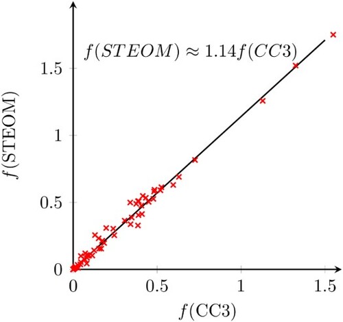
For the total set of 92 states, the CC3 and STEOM excitation energy values are in good agreement, the mean error and standard deviation of the STEOM results being $-0.02\pm 0.10$ eV, with a maximum absolute error of 0.32 eV. It should be remarked that two of the Rydberg states produce an error larger than 0.15 eV, although these are by no means the only large errors in the test set, the largest one corresponding to an $n\to {\pi }^{\ast }$ excitation of thymine. To characterise the oscillator strengths computed at the various levels, they are plotted against each other in Figure 1 and the various linear regression results are provided in Table 4. Plotting the STEOM-CIS results against the CC3 ones, it is immediately clear that this approximation overestimates the CC3 densities by about 59% on average. However, the linear fit is quite good even in this case ($R^2=0.965$), and since the intercept parameter b is very small, this amounts effectively to a scaling of the CC3 values. Since in applications it is often the relative intensities that matter, we conclude that the CIS approximation to the STEOM density that we have used so far can be expected to yield reliable results for relative intensities. Turning to the full STEOM density, the extent of the overestimation is reduced to about 14%, and the quality of the fit is somewhat better ($R^2=0.990$). This is in excellent agreement with CC3 results, especially considering the much reduced cost of an STEOM calculation when compared to CC3. Plotting the two STEOM densities against each other, it turns out that the full STEOM density yields an oscillator strength that is on average 70% of the CIS approximation and the correlation between the two is also very good ($R^2=0.980$). Nevertheless, the full density with the L2 correction is a significant improvement over the simple CIS formula and is set as the new default for STEOM calculations in ORCA. Finally, the last columns of Tables 2 and  3 also contain data on the more expensive STEOM-DD correction. Computing the linear regression parameters for STEOM-DD shows a slightly better agreement with CC3 values, the oscillator strength values being about 8% overestimated with $R^2=0.990$. The STEOM-DD values for the ground state dipole moments are tabulated in the supplementary material, and also yield good agreement with reference values. The improvement over the full STEOM density with the L2 correction is however negligible for transition dipoles, while the additional costs are considerable. Thus, especially for large molecules, we recommend skipping the DD correction since the increase in cost can be especially large. An intermediate solution is to update the L1 amplitudes only according to Equation (36(36) ${\overline{L}}_1^{†}={\hat{L}}_1^{†}-{\hat{L}}_2^{†}\hat{S}.$(36) ). While this still requires the explicit construction of the L2 amplitudes, the contractions involved are cheaper, and according to the oscillator strength values tabulated in the supplementary material, essentially all the improvements of STEOM-DD can be recovered by correcting L1 only. Thus, this correction may be recommended, if affordable.

Figure 1. Comparison of oscillator strength values computed at the CIS, STEOM-CCSD and CC3 levels.

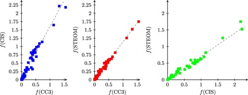
Table 4. Linear regression results (y = ax + b) corresponding to Figure 1, Table 2 and Table 3.

x	y	a	b	$R^2$
f(CC3)	f(CIS)	1.5851	0.0162	0.9653
f(CC3)	f(STEOM)	1.1359	0.0041	0.9903
f(CIS)	f(STEOM)	0.7006	−0.0026	0.9805
f(CC3)	f(STEOM-DD)	1.0826	0.0025	0.9908

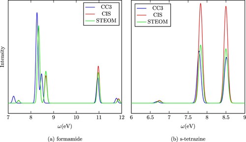
To illustrate the performance of the CIS approximation and the full density, two theoretical spectra are shown in Figure 2. The spectrum of formamide is an example for which using the full density has a relatively small effect, the CIS and full density spectra are close to each other and to the CC3 curve also. On the other hand, the case of s-tetrazine demonstrates the impact of the full density well. In this case, the full density and CC3 curves are close to one another while the CIS curve significantly overestimates the intensity.

Figure 2. The spectra of two selected species from Thiel's test set.

5. Conclusions

In this study, we have derived and implemented a STEOM density that improves on the simplest CIS approximation for computing transition properties, without demanding the same cost as a density calculation within the space of the singles and the doubles. We concluded that although the CIS formula is a good approximation in may practical applications, the full STEOM density with the L2 correction offers an improvement without much additional cost. The oscillator strength values obtained from this density correlate well with CC3 results, and thus the STEOM method not only yields reliable results for the excitation energy, but it can be used to reproduce and interpret experimental spectra.

Disclosure statement

No potential conflict of interest was reported by the author(s).

Additional information

Funding

This work was supported by the Max-Planck-Gesellschaft.

References

- J. Gauss, in Encyclopedia of Computational Chemistry (John Wiley and Sons, Chichester, 2002), p. 615.
- R.J. Bartlett, Wiley Interdiscip. Rev.: Comput. Molecular Sci. 2 (1), 126–138 (2012). doi: 10.1002/wcms.76
- D.I. Lyakh, M. Musiał, V.F. Lotrich, and R.J. Bartlett, Chem. Rev. 112 (1), 182–243 (2012). doi:10.1021/cr2001417
- A. Köhn, M. Hanauer, L.A. Mück, T.C. Jagau, and J. Gauss, WIREs Comput. Molecular Sci. 3 (2), 176–197 (2013). doi:10.1002/wcms.1120
- U.S. Mahapatra, B. Datta, and D. Mukherjee, J. Chem. Phys. 110 (13), 6171–6188 (1999). doi:10.1063/1.478523
- T.C. Jagau and J. Gauss, J. Chem. Phys. 137 (4), 044116 (2012). doi:10.1063/1.4734309
- K. Emrich, Nucl. Phys. A 351 (3), 379–396 (1981). doi:10.1016/0375-9474(81)90179-2
- J.F. Stanton and R.J. Bartlett, J. Chem. Phys. 98 (9), 7029–7039 (1993). doi:10.1063/1.464746
- R. Izsák, WIREs Comput. Molecular Sci. 10 (3), e1445. (2019).
- O. Christiansen, H. Koch, and P. Jørgensen, Chem. Phys. Lett. 243 (5), 409–418 (1995). doi:10.1016/0009-2614(95)00841-Q
- M. Nooijen and J.G. Snijders, J. Chem. Phys. 102 (4), 1681–1688 (1995). doi:10.1063/1.468900
- J.F. Stanton and J. Gauss, J. Chem. Phys. 103 (3), 1064–1076 (1995). doi:10.1063/1.469817
- A.K. Dutta, J. Gupta, H. Pathak, N. Vaval, and S. Pal, J. Chem. Theory. Comput. 10 (5), 1923–1933 (2014). doi:10.1021/ct4009409
- A.B. Trofimov, I.L. Krivdina, J. Weller, and J. Schirmer, Chem. Phys. 329 (1–3), 1–10 (2006). doi:10.1016/j.chemphys.2006.07.015
- C. Hättig, in Computational Nanoscience: Do It Yourself (John von Neumann Institute for Computing, Juelich, 2006), Vol 31, pp. 245–278.
- C. Hättig and F. Weigend, J. Chem. Phys. 113 (13), 5154–5161 (2000). doi:10.1063/1.1290013
- E. Epifanovsky, D. Zuev, X. Feng, K. Khistyaev, Y. Shao, and A.I. Krylov, J. Chem. Phys. 139 (13), 134105 (2013). doi:10.1063/1.4820484
- A.K. Dutta, F. Neese, and R. Izsák, J. Chem. Phys. 144 (3), 034102 (2016). doi:10.1063/1.4939844
- E.G. Hohenstein, S.I.L. Kokkila, R.M. Parrish, and T.J. Martínez, J. Phys. Chem. B 117 (42), 12972–12978 (2013). doi:10.1021/jp4021905
- T. Korona and H.J. Werner, J. Chem. Phys. 118 (7), 3006–3019 (2003). doi:10.1063/1.1537718
- A.K. Dutta, F. Neese, and R. Izsák, J. Chem. Phys. 145 (3), 034102 (2016). doi:10.1063/1.4958734
- M.S. Frank and C. Hättig, J. Chem. Phys. 148 (13), 134102 (2018). doi:10.1063/1.5018514
- C. Peng, M.C. Clement, and E.F. Valeev, J. Chem. Theory. Comput. 14 (11), 5597–5607 (2018). doi:10.1021/acs.jctc.8b00171
- P. Baudin and K. Kristensen, J. Chem. Phys. 144 (22), 224106 (2016). doi:10.1063/1.4953360
- S. Höfener and W. Klopper, Chem. Phys. Lett. 679 (Supplement C), 52–59 (2017). doi:10.1016/j.cplett.2017.04.083
- I.M. Hoyvik, R.H. Myhre, and H. Koch, J. Chem. Phys 146 (14), 144109 (2017). doi:10.1063/1.4979908
- D. Mester, P.R. Nagy, and M. Kallay, J. Chem. Phys. 146 (19), 194102 (2017). doi:10.1063/1.4983277
- Y.C. Park, A. Perera, and R.J. Bartlett, J. Chem. Phys. 149 (18), 184103 (2018). doi:10.1063/1.5045340
- M. Nooijen and R.J. Bartlett, J. Chem. Phys. 107 (17), 6812–6830 (1997). doi:10.1063/1.474922
- L.Z. Stolarczyk and H.J. Monkhorst, Phys. Rev. A 32, 725–742 (1985). doi:10.1103/PhysRevA.32.725
- L.Z. Stolarczyk and H.J. Monkhorst, Mol. Phys. 108 (21-23), 3067–3089 (2010). doi:10.1080/00268976.2010.518981
- S. Pal, M. Rittby, R.J. Bartlett, D. Sinha, and D. Mukherjee, J. Chem. Phys. 88 (7), 4357–4366 (1988). doi:10.1063/1.453795
- L. Meissner, J. Chem. Phys. 108 (22), 9227–9235 (1998). doi:10.1063/1.476377
- A.K. Dutta, J. Gupta, N. Vaval, and S. Pal, J. Chem. Theory. Comput. 10 (9), 3656–3668 (2014). doi:10.1021/ct500285e
- A.K. Dutta, M. Nooijen, F. Neese, and R. Izsák, J. Chem. Phys. 146 (7), 074103 (2017). doi:10.1063/1.4976130
- A.K. Dutta, M. Nooijen, F. Neese, and R. Izsák, J. Chem. Theory. Comput. 14 (1), 72–91 (2018). doi:10.1021/acs.jctc.7b00802
- D. Bokhan, D.N. Trubnikov, and R.J. Bartlett, J. Chem. Phys. 143 (7), 074111 (2015). doi:10.1063/1.4928736
- D. Bokhan, D.N. Trubnikov, A. Perera, and R.J. Bartlett, J. Chem. Phys. 151 (13), 134110 (2019). doi:10.1063/1.5121373
- L.M.J. Huntington, M. Krupička, F. Neese, and R. Izsák, J. Chem. Phys. 147 (17), 174104 (2017). doi:10.1063/1.5001320
- A. Dittmer, R. Izsák, F. Neese, and D. Manganas, Inorg. Chem. 58 (14), 9303–9315 (2019). doi:10.1021/acs.inorgchem.9b00994
- J. Arponen, Ann. Phys. (N. Y) 151 (2), 311–382 (1983). doi:10.1016/0003-4916(83)90284-1
- H. Koch, H.J.A. Jensen, P. Jørgensen, T. Helgaker, G.E. Scuseria, and H.F. Schaefer, J. Chem. Phys. 92 (8), 4924–4940 (1990). doi:10.1063/1.457710
- J. Gauss, in Modern Methods and Algorithms of Quantum Chem (John von Neumann Institute for Computing, Juelich, 2000), Vol. 1, pp. 509–560.
- J. Gauss, J.F. Stanton, and R.J. Bartlett, J. Chem. Phys. 95 (4), 2623–2638 (1991). doi:10.1063/1.460915
- J.F. Stanton and J. Gauss, Int. Rev. Phys. Chem. 19 (1), 61–95 (2000). doi:10.1080/014423500229864
- L. Cheng, S. Stopkowicz, and J. Gauss, Int. J. Quantum. Chem. 114 (17), 1108–1127 (2014). doi:10.1002/qua.24636
- P.G. Szalay and J. Gauss, J. Chem. Phys. 112 (9), 4027–4036 (2000). doi:10.1063/1.480952
- M. Kállay and J. Gauss, J. Chem. Phys. 121 (19), 9257–9269 (2004). doi:10.1063/1.1805494
- J.F. Stanton and J. Gauss, J. Chem. Phys. 100 (6), 4695–4698 (1994). doi:10.1063/1.466253
- H. Koch, R. Kobayashi, A.S. de Merás, and P. Jørgensen, J. Chem. Phys. 100 (6), 4393–4400 (1994). doi:10.1063/1.466321
- K.D. Nanda and A.I. Krylov, J. Chem. Phys. 145 (20), 204116 (2016). doi:10.1063/1.4967860
- D. Bhattacharya, N. Vaval, and S. Pal, J. Chem. Phys. 138 (9), 094108 (2013). doi:10.1063/1.4793277
- S.R. Gwaltney, R.J. Bartlett, and M. Nooijen, J. Chem. Phys. 111 (1), 58–64 (1999). doi:10.1063/1.479361
- M. Wladyslawski and M. Nooijen, in Advances in Quantum Chemistry, edited by J.R. Sabin and E. Brändas (Elsevier, Amsterdam, 2005), Vol. 49, pp. 1–101.
- A. Landau, J. Chem. Phys. 139 (1), 014110 (2013). doi:10.1063/1.4811799
- R. Berraud-Pache, F. Neese, G. Bistoni, and R. Izsák, J. Chem. Theory. Comput. 16 (1), 564–575 (2020). doi:10.1021/acs.jctc.9b00559
- C. Kollmar and F. Neese, J. Chem. Phys. 135 (6), 064103 (2011). doi:10.1063/1.3618720
- A.K. Dutta, F. Neese, and R. Izsák, J. Chem. Phys. 146 (21), 214111 (2017). doi:10.1063/1.4984618
- M. Schreiber, M.R. Silva-Junior, S.P.A. Sauer, and W. Thiel, J. Chem. Phys. 128 (13), 134110 (2008). doi:10.1063/1.2889385
- J. Sous, P. Goel, and M. Nooijen, Mol. Phys. 112 (5–6), 616–638 (2014). doi:10.1080/00268976.2013.847216
- D. Kánnár, and P.G. Szalay, J. Chem. Theory. Comput. 10 (9), 3757–3765 (2014). doi:10.1021/ct500495n
- A. Schäfer, H. Horn, and R. Ahlrichs, J. Chem. Phys. 97 (4), 2571–2577 (1992). doi:10.1063/1.463096
- H. Koch, O. Christiansen, P. Jørgensen, A.M. Sanchez de Merás, and T. Helgaker, J. Chem. Phys.106 (5), 1808–1818 (1997). doi:10.1063/1.473322
- F. Neese, Wiley Interdiscip. Rev.: Comput. Molecular Sci. 8 (1), e1327 (2017). doi: 10.1002/wcms.1327