Density functional study of non-isothermal hard sphere fluids

ABSTRACT

Using a version of dynamical density functional theory, we explore a microscopic structure of hard-sphere fluids in the presence of a temperature gradient. When combined with the assumption of local equilibrium, this approach predicts the density profile in confinement and in bulk both in very good overall agreement with the results from the reverse non-equilibrium molecular dynamics simulation, which we used to impose a temperature gradient. Thus, the assumption of local equilibrium is found to be surprisingly accurate down to a microscopic scale even under a large temperature gradient. An oscillatory density profile, indicating the layering of particles, was observed in bulk as well as in confinement. This behaviour in the latter is well known and results from packing of hard spheres next to a wall. In the former, the oscillation is seen to emanate from the point of sharp change in temperature. However, our theoretical predictions greatly exaggerate the amplitude of oscillation when the temperature exhibits a sharp change over a very small distance.

GRAPHICAL ABSTRACT

Keywords:

• Dynamical density functional theory
• heat conduction
• local equilibrium
• reverse non-equilibrium molecular dynamics
• hard spheres

1. Introduction

Since its inception, statistical mechanical density functional theory (DFT) [1] has been applied successfully to probe phase behaviour and microscopic structures of fluids [2] from a molecular level perspective while requiring a fraction of a typical computational cost of molecular-level simulations. DFT provides much easier access to an activated state (in unstable equilibrium) involved in a rare event such as nucleation [3,4]. It can also offer deep insights that are otherwise unavailable into physics of inhomogeneous systems.

While the original DFT is applicable only to systems in equilibrium, a considerable progress has been made in recent years to extend DFT to non-equilibrium systems. The earliest of such attempts focused on the time evolution of the density profile, [5,6] resulting in a dynamical density functional theory (DDFT) suitable for describing diffusion processes only. The scope of DDFT has since been expanded by including additional fields in its formulation.

Broadly speaking, DDFT has been developed following two distinct approaches. The starting point for the first approach [7–17] is the lowest order equation in the Bogoliubov–Born–Green–Kirkwood–Yvon hierarchy [18], which dictates the time evolution of the single particle distribution function $f_1(\mathbf{r},\mathbf{v},t)$, expressing the probability density of finding a particle at $\mathbf{r}$ with velocity $\mathbf{v}$ at time t. The equations of motion for the density, momentum, and energy (or temperature) fields are obtained by averaging proper microscopic expressions for these quantities with respect to $f_1(\mathbf{r},\mathbf{v},t)$. This is essentially the Irving–Kirkwood procedure [19] and gives rise to integrals involving the pair distribution function $f_2(\mathbf{r},\mathbf{v},{\mathbf{r}}^{\mathrm{\prime }},{\mathbf{v}}^{\mathrm{\prime }},t)$, the probability density of finding a pair of particles, one at $(\mathbf{r},\mathbf{v})$ and the other at $({\mathbf{r}}^{\mathrm{\prime }},{\mathbf{v}}^{\mathrm{\prime }})$ at time t. To evaluate these integrals, one must introduce various approximations typically informed by recent techniques from the kinetic theory [20–23].

The second approach [24–26] is based on the time-dependent projection operator method [27]. Here, one must first specify a set of relevant macrovariables based on physics. For transport phenomena, they are particle number (or mass) density, velocity, and energy density fields. Specification of these fields does not uniquely determine the actual phase-space distribution $\varrho ({\mathbf{r}}^N,{\mathbf{p}}^N,t)$ for a system in a non-equilibrium state. Nevertheless, the least biased distribution $\overline{\varrho }({\mathbf{r}}^N,{\mathbf{p}}^N,t)$ compatible with the given fields can be determined by maximising the Gibbs entropy associated with $\overline{\varrho }$ under the constraint that $\overline{\varrho }({\mathbf{r}}^N,{\mathbf{p}}^N,t)$ gives rise to the specified fields [28]. The end result is a time-dependent generalised canonical distribution, from which one obtains the entropy functional and the transport equations that dictate the time evolution of the fields. The difference between $\overline{\varrho }$ and ϱ is reflected in the equations of motion for fluctuations of the fields. This method also yields molecular level expressions for transport coefficients in the form of the Green–Kubo formula. These results are formally exact.

The explicit connection to the entropy functional established in the second formulation may allow for a wealth of knowledge accumulated in the equilibrium DFT to be most easily incorporated into DDFT, thus leading to a systematic generalisation of DDFT to complex fluids. In this scenario, hard-sphere fluids will serve almost exclusively as a reference system. Thus, it is important that DDFT be capable of describing their properties and microstructure accurately under various non-equilibrium conditions.

As with the equilibrium DFT, the generalised DDFT showed its ability to predict accurately the density profiles in confined fluids for isothermal systems [6,10]. To our knowledge, however, a similar verification is lacking for non-isothermal systems. As an initial step toward DDFT of complex fluids, we explored microstructures of non-isothermal hard-sphere fluids using a version of DDFT put forward by Anero et al. [26].

Combining the entropy functional of hard spheres derived in [26] with the assumption of local equilibrium, which is routinely invoked in arriving at the governing equations of macroscopic hydrodynamics [29,30], we predict the density profile across a hard-sphere fluid both in a confined space defined by two parallel plates and in bulk in the presence of a temperature gradient. As expected, packing of hard spheres in strong confinement produces an oscillatory density profile (indicating a layering of the particles). When temperature gradient is generated by the method called the reverse non-equilibrium molecular dynamics (RNEMD) [31], a strongly oscillatory density profile was observed in the bulk system without any confinement. In a separate simulation, we used RNEMD to impose a simple shear flow, which resulted in a non-uniform temperature profile. In all cases, our theoretical predictions are in very good overall agreement with the results of molecular simulation, thus providing a strong indication in favour of the local equilibrium assumption at the microscopic length scale. However, DDFT was seen to greatly exaggerate the oscillatory behaviour when the temperature exhibits a sharp change over a very small distance.

The remainder of this article is structured as follows. Section 2 summarises the relevant results from  [26]. The equation for the density profile is derived in Section 3, while details of RNEMD simulation is given in Section 4. The results of our computations are reported in Section 5 and the article concludes with a brief summary in Section 6. Appendix 1 records a set of key equations from Rosenfeld's fundamental measure theory [32–34], which we used to estimate the excess Helmholtz free energy of a hard-sphere fluid. Appendix 2 establishes the formula we used to construct the temperature profile from a simulation in the presence of a convective motion.

2. Dynamical density functional theory

Assuming that density and energy density profiles, to be denoted by $\rho (\mathbf{r},t)$ and $e(\mathbf{r},t)$, respectively, are the only relevant fields, Anero et al. developed a version of DDFT [26] by means of the time-dependent projection operator method [27]. Their key results pertaining to the current work are as follows.

The entropy of a system consisting of hard spheres of radius σ and mass m is given as a functional of $\rho (\mathbf{r},t)$ and $e(\mathbf{r},t)$ by (1) $\begin{array}{rl}S/k_{\mathrm{B}}[\rho ,e]& =-\int \rho (\mathbf{r})[\frac{5}{2}\ln \rho (\mathbf{r},t)-\frac{3}{2}\ln e(\mathbf{r},t)\\ & +\ln {\alpha }^3-\frac{5}{2}]\mathrm{d}\mathbf{r}-\int \mathrm{\Phi }[\rho ;\mathbf{r},t)\mathrm{d}\mathbf{r},\end{array}$(1) where α is related to the thermal wavelength Λ by (2) $\alpha :={\left(\frac{3h^2}{4\pi m}\right)}^{1/2}={\left(\frac{3}{2k_{\mathrm{B}}T(\mathbf{r},t)}\right)}^{1/2}\mathrm{\Lambda }(\mathbf{r},t),$(2) in which h and $k_B$ denote the Planck and Boltzmann constants, respectively, and $\mathrm{\Phi }[\rho ;\mathbf{r},t)$ is the excess Helmholtz free energy per unit volume of the hard-sphere fluid in $k_{\mathrm{B}}T$ units.

As the notation suggests, Φ is a functional of the density profile $\rho (\mathbf{r},t)$ and a function of $\mathbf{r}$ and t. This functional dependence arises when we use ($\mathbf{r}$ and t dependent) weighted densities to compute Φ.

The time evolution of ρ and e are governed by the following transport equations [26]: (3) $\begin{array}{rl}\frac{\mathrm{\partial }\rho (\mathbf{r},t)}{\mathrm{\partial }t}+\mathrm{\nabla }\cdot {\mathbf{J}}^{\rho }& =0,\\ \frac{\mathrm{\partial }e(\mathbf{r},t)}{\mathrm{\partial }t}+\mathrm{\nabla }\cdot {\mathbf{J}}^e& =0.\end{array}$(3) where ${\mathbf{J}}^{\rho }$ and ${\mathbf{J}}^e$ are given by (4) $\begin{array}{rl}{\mathbf{J}}^{\rho }& :=D(\mathbf{r},t)\mathrm{\nabla }\frac{\delta S/k_{\mathrm{B}}}{\delta \rho (\mathbf{r},t)}+C(\mathbf{r},t)\mathrm{\nabla }\frac{\delta S/k_{\mathrm{B}}}{\delta e(\mathbf{r},t)},\\ {\mathbf{J}}^e& :=C(\mathbf{r},t)\mathrm{\nabla }\frac{\delta S/k_{\mathrm{B}}}{\delta \rho (\mathbf{r},t)}+K(\mathbf{r},t)\mathrm{\nabla }\frac{\delta S/k_{\mathrm{B}}}{\delta e(\mathbf{r},t)}\end{array}$(4) and represent particle and energy flux vectors, respectively. The functions C, D, and K are transport coefficients that need to be determined by molecular dynamics (MD) simulations.

As shown in [26], (5) $\frac{\delta S/k_{\mathrm{B}}}{\delta e(\mathbf{r},t)}=\beta (\mathbf{r},t):=\frac{1}{k_{\mathrm{B}}T(\mathbf{r})}$(5) in general. For the entropy functional given by Equation (1(1) $\begin{array}{rl}S/k_{\mathrm{B}}[\rho ,e]& =-\int \rho (\mathbf{r})[\frac{5}{2}\ln \rho (\mathbf{r},t)-\frac{3}{2}\ln e(\mathbf{r},t)\\ & +\ln {\alpha }^3-\frac{5}{2}]\mathrm{d}\mathbf{r}-\int \mathrm{\Phi }[\rho ;\mathbf{r},t)\mathrm{d}\mathbf{r},\end{array}$(1) ), this leads to (6) $\frac{3\rho (\mathbf{r},t)}{2e(\mathbf{r},t)}=\beta (\mathbf{r},t),$(6) which is expected since the internal energy of a hard-sphere fluid consists only of the kinetic energy. Carrying out the functional derivative with respect to $\rho (\mathbf{r},t)$, (7) $\begin{array}{rl}-\frac{\delta S/k_{\mathrm{B}}}{\delta \rho (\mathbf{r},t)}& =\frac{5}{2}\ln \rho (\mathbf{r},t)-\frac{3}{2}\ln e(\mathbf{r},t)+\ln {\alpha }^3\\ & +\frac{\delta }{\delta \rho (\mathbf{r},t)}\int \mathrm{\Phi }[\rho ;\mathbf{r},t)\mathrm{d}\mathbf{r}\\ & =\ln [{\mathrm{\Lambda }}^3(\mathbf{r},t)\rho (\mathbf{r},t)]\\ & +\frac{\delta }{\delta \rho (\mathbf{r},t)}\int \mathrm{\Phi }[\rho ;\mathbf{r},t)\mathrm{d}\mathbf{r}\\ & =\lambda (\mathbf{r},t),\end{array}$(7) where we defined λ by the expression preceding it. More accurately, $-\lambda$ arises as a field conjugate to ρ when one employs the generalised canonical ensemble for the relevant phase distribution of a non-equilibrium system [26,27]. The same comment applies to the pair of fields β and e. We observe that $\lambda (\mathbf{r},t)$ reduces to $\beta \mu$ (a constant) with μ denoting the chemical potential if the system is in equilibrium.

3. One-dimensional problems

In what follows, we shall limit ourselves to a steady-state one-dimensional problem in a rectangular coordinate system and consider, initially, a stationary fluid. Taking the z-axis in the direction of the temperature gradient, ρ and e are now functions only of z. In this case, Equation (3(3) $\begin{array}{rl}\frac{\mathrm{\partial }\rho (\mathbf{r},t)}{\mathrm{\partial }t}+\mathrm{\nabla }\cdot {\mathbf{J}}^{\rho }& =0,\\ \frac{\mathrm{\partial }e(\mathbf{r},t)}{\mathrm{\partial }t}+\mathrm{\nabla }\cdot {\mathbf{J}}^e& =0.\end{array}$(3) ) indicates that the z-components $J_z^{\rho }$ and $J_z^e$ are both constant. Even then, the solution of the resulting equations requires knowledge of the transport coefficients C, D, and K, which are in general functions of position and their evaluation even by a computer simulation is possible only with further simplifying assumptions. In the problem under consideration, however, the issue can be circumvented as we now discuss.

First, in the formulation of [26], the velocity profile is not included in the list of relevant variables. In the case of a stationary fluid, however, the velocity field being identically zero carries an important information, which a more general formulation of DDFT is expected to provide. For the problems under consideration here, we shall take it for granted that the lack of convective motion implies the uniformity of the pressure field $p(\mathbf{r})$: (8) $\mathrm{\nabla }p\equiv \mathbf{0}.$(8) Note that this identity is certainly violated if a spherical interface separates two fluid phases as is evident from the Laplace equation.

Second, we assume that the local equilibrium prevails everywhere in the system. This implies that $\lambda (\mathbf{r},t)$ defined by Equation (7(7) $\begin{array}{rl}-\frac{\delta S/k_{\mathrm{B}}}{\delta \rho (\mathbf{r},t)}& =\frac{5}{2}\ln \rho (\mathbf{r},t)-\frac{3}{2}\ln e(\mathbf{r},t)+\ln {\alpha }^3\\ & +\frac{\delta }{\delta \rho (\mathbf{r},t)}\int \mathrm{\Phi }[\rho ;\mathbf{r},t)\mathrm{d}\mathbf{r}\\ & =\ln [{\mathrm{\Lambda }}^3(\mathbf{r},t)\rho (\mathbf{r},t)]\\ & +\frac{\delta }{\delta \rho (\mathbf{r},t)}\int \mathrm{\Phi }[\rho ;\mathbf{r},t)\mathrm{d}\mathbf{r}\\ & =\lambda (\mathbf{r},t),\end{array}$(7) ) may be identified as $\beta \mu$ at position $\mathbf{r}$ and that the Gibbs–Duhem relation may be applied at every $\mathbf{r}$ even though the system under consideration is not in equilibrium. Thus, (9) $e\frac{\mathrm{d}\beta }{\mathrm{d}z}+\frac{\mathrm{d}(\beta p)}{\mathrm{d}z}-\rho \frac{\mathrm{d}\lambda }{\mathrm{d}z}=0.$(9) Using Equation (8(8) $\mathrm{\nabla }p\equiv \mathbf{0}.$(8) ), (10) $\chi \frac{\mathrm{d}\beta }{\mathrm{d}z}-\rho \frac{\mathrm{d}\lambda }{\mathrm{d}z}=0.$(10) where $\chi :=e+p$ is the enthalpy density. By means of this equation, we rewrite Equation (4(4) $\begin{array}{rl}{\mathbf{J}}^{\rho }& :=D(\mathbf{r},t)\mathrm{\nabla }\frac{\delta S/k_{\mathrm{B}}}{\delta \rho (\mathbf{r},t)}+C(\mathbf{r},t)\mathrm{\nabla }\frac{\delta S/k_{\mathrm{B}}}{\delta e(\mathbf{r},t)},\\ {\mathbf{J}}^e& :=C(\mathbf{r},t)\mathrm{\nabla }\frac{\delta S/k_{\mathrm{B}}}{\delta \rho (\mathbf{r},t)}+K(\mathbf{r},t)\mathrm{\nabla }\frac{\delta S/k_{\mathrm{B}}}{\delta e(\mathbf{r},t)}\end{array}$(4) ) as (11) $\begin{array}{rl}{J}_z^{\rho }& =(C-D\frac{\chi }{\rho })\frac{\mathrm{d}\beta }{\mathrm{d}z},\\ J_z^e& =(K-C\frac{\chi }{\rho })\frac{\mathrm{d}\beta }{\mathrm{d}z},\end{array}$(11) Finally, $J_z^{\rho }\equiv 0$ in a stationary single component system. In the presence of non-zero temperature gradient, $\mathrm{d}\beta /\mathrm{d}z\ne 0$ and hence (12) $C-D\frac{\chi }{\rho }=0.$(12) This can be used in Equation (11(11) $\begin{array}{rl}{J}_z^{\rho }& =(C-D\frac{\chi }{\rho })\frac{\mathrm{d}\beta }{\mathrm{d}z},\\ J_z^e& =(K-C\frac{\chi }{\rho })\frac{\mathrm{d}\beta }{\mathrm{d}z},\end{array}$(11) ) to give (13) $j_z^e=-\frac{1}{k_{\mathrm{B}}{T}^2}[K-D{\left(\frac{\chi }{\rho }\right)}^2]\frac{\mathrm{d}T}{\mathrm{d}z},$(13) in which we recognise (14) $\kappa :=\frac{1}{k_{\mathrm{B}}{T}^2}[K-D{\left(\frac{\chi }{\rho }\right)}^2]$(14) as the thermal conductivity.

In many situations, κ may be regarded as constant and Equation (13(13) $j_z^e=-\frac{1}{k_{\mathrm{B}}{T}^2}[K-D{\left(\frac{\chi }{\rho }\right)}^2]\frac{\mathrm{d}T}{\mathrm{d}z},$(13) ) can be integrated to give a linear temperature profile. As we shall see below, our simulation indicates that the temperature profile is indeed linear over a large section of the system even though the system as a whole is inhomogeneous.

In any event, let us now proceed under the assumption that $T(z)$ is known. From Equation (10(10) $\chi \frac{\mathrm{d}\beta }{\mathrm{d}z}-\rho \frac{\mathrm{d}\lambda }{\mathrm{d}z}=0.$(10) ), (15) $\frac{\mathrm{d}\lambda }{\mathrm{d}z}=\frac{\chi }{\rho }\frac{\mathrm{d}\beta }{\mathrm{d}z}=-\frac{\chi }{\rho k_{\mathrm{B}}{T}^2}\frac{\mathrm{d}T}{\mathrm{d}z},$(15) Upon integration from z = 0, which we shall take at the centre of the system, we arrive at (16) $\lambda (z)=\lambda (0)-{\int }_{T(0)}^{T(z)}\frac{\chi }{\rho k_{\mathrm{B}}{T}^2}\mathrm{d}T,$(16) Using Equation (7(7) $\begin{array}{rl}-\frac{\delta S/k_{\mathrm{B}}}{\delta \rho (\mathbf{r},t)}& =\frac{5}{2}\ln \rho (\mathbf{r},t)-\frac{3}{2}\ln e(\mathbf{r},t)+\ln {\alpha }^3\\ & +\frac{\delta }{\delta \rho (\mathbf{r},t)}\int \mathrm{\Phi }[\rho ;\mathbf{r},t)\mathrm{d}\mathbf{r}\\ & =\ln [{\mathrm{\Lambda }}^3(\mathbf{r},t)\rho (\mathbf{r},t)]\\ & +\frac{\delta }{\delta \rho (\mathbf{r},t)}\int \mathrm{\Phi }[\rho ;\mathbf{r},t)\mathrm{d}\mathbf{r}\\ & =\lambda (\mathbf{r},t),\end{array}$(7) ), we may rewrite (16(16) $\lambda (z)=\lambda (0)-{\int }_{T(0)}^{T(z)}\frac{\chi }{\rho k_{\mathrm{B}}{T}^2}\mathrm{d}T,$(16) ) as (17) $\rho (z)={\left[\frac{T(z)}{T(0)}\right]}^{3/2}{\rho }_0{\mathrm{e}}^{-B[\rho ;z)},$(17) which may be solved by iteration. Here, we defined (18) $B[\rho ;z):={[\frac{\delta }{\delta \rho (z)}\int \mathrm{\Phi }[\rho ;z)\mathrm{d}z]}_0^z+{\int }_{T(0)}^{T(z)}\frac{\chi }{\rho k_{\mathrm{B}}{T}^2}\mathrm{d}T.$(18) Equation (1(1) $\begin{array}{rl}S/k_{\mathrm{B}}[\rho ,e]& =-\int \rho (\mathbf{r})[\frac{5}{2}\ln \rho (\mathbf{r},t)-\frac{3}{2}\ln e(\mathbf{r},t)\\ & +\ln {\alpha }^3-\frac{5}{2}]\mathrm{d}\mathbf{r}-\int \mathrm{\Phi }[\rho ;\mathbf{r},t)\mathrm{d}\mathbf{r},\end{array}$(1) ) implies the interpretation of the quantity (19) $\begin{array}{rl}(s/k_{\mathrm{B}})[\rho ;\mathbf{r},t)& =-\rho (\mathbf{r},t)[\frac{5}{2}\ln \rho (\mathbf{r},t)-\frac{3}{2}\ln e(\mathbf{r},t)\\ & +\ln {\alpha }^3-\frac{5}{2}]-\mathrm{\Phi }[\rho ;\mathbf{r},t)\end{array}$(19) as the entropy density. Using Equations (7(7) $\begin{array}{rl}-\frac{\delta S/k_{\mathrm{B}}}{\delta \rho (\mathbf{r},t)}& =\frac{5}{2}\ln \rho (\mathbf{r},t)-\frac{3}{2}\ln e(\mathbf{r},t)+\ln {\alpha }^3\\ & +\frac{\delta }{\delta \rho (\mathbf{r},t)}\int \mathrm{\Phi }[\rho ;\mathbf{r},t)\mathrm{d}\mathbf{r}\\ & =\ln [{\mathrm{\Lambda }}^3(\mathbf{r},t)\rho (\mathbf{r},t)]\\ & +\frac{\delta }{\delta \rho (\mathbf{r},t)}\int \mathrm{\Phi }[\rho ;\mathbf{r},t)\mathrm{d}\mathbf{r}\\ & =\lambda (\mathbf{r},t),\end{array}$(7) ) and (19(19) $\begin{array}{rl}(s/k_{\mathrm{B}})[\rho ;\mathbf{r},t)& =-\rho (\mathbf{r},t)[\frac{5}{2}\ln \rho (\mathbf{r},t)-\frac{3}{2}\ln e(\mathbf{r},t)\\ & +\ln {\alpha }^3-\frac{5}{2}]-\mathrm{\Phi }[\rho ;\mathbf{r},t)\end{array}$(19) ), and the Euler relation, (20) $\begin{array}{rl}\beta \chi & =s/k_{\mathrm{B}}+\lambda \rho \\ & =\rho [\frac{5}{2}+\frac{\delta }{\delta \rho (z)}\int \mathrm{\Phi }[\rho ;z)\mathrm{d}z]-\mathrm{\Phi }[\rho ;z).\end{array}$(20) To capture the microstructure of hard-sphere fluids as accurately as possible, we evaluate Φ and the functional derivative of its integral using the dimensional interpolation version [33] of the fundamental measure theory [32] specialised to one-dimensional problems. Key formulas are listed in Appendix 1.

The notion of local equilibrium is distinct from that of the local density approximation. In the latter, the entropy density at $\mathbf{r}$ is given as a function of density evaluated at the same position $\mathbf{r}$. In the fundamental measure theory, Φ is expressed as a function of three weighted densities, making Φ at $\mathbf{r}$ dependent on the density profile within the sphere of radius σ centred around $\mathbf{r}$. Oscillatory density profiles shown in Section 5 could not be predicted with the local density approximation.

4. Simulation

In what follows, we adopt a system of units in which m = 1 and $\sigma =0.5$. As is customary in MD simulations, the total linear momentum of the system is set to zero. Motivated by the equipartition theorem for an isothermal system in equilibrium, we define the overall system temperature $k_{\mathrm{B}}\overline{T}$ by (21) $\sum _{i=1}^N\frac{1}{2}||{\mathbf{v}}_i|{|}^2=\frac{3}{2}(N-1)k_{\mathrm{B}}\overline{T},$(21) where N is the number of particles in the system and ${\mathbf{v}}_i$ is the velocity of the ith particle. Since a hard-sphere fluid does not have potential energy, the total kinetic energy is conserved exactly in molecular dynamics. Accordingly, we have written Equation (21(21) $\sum _{i=1}^N\frac{1}{2}||{\mathbf{v}}_i|{|}^2=\frac{3}{2}(N-1)k_{\mathrm{B}}\overline{T},$(21) ) without time or ensemble averaging. We set $k_{\mathrm{B}}\overline{T}=1$ and this determines the energy scale.

Our simulation box is a rectangular block of a square base of area A and height $2H$. To simulate a confined fluid, we placed hard walls as shown in Figure 1(a). In the coordinate system with its origin at the centre of the simulation box and the z-axis perpendicular to the opposing square faces of the box, they are at $|z|=H$, thus restricting the centres of hard spheres to $|z|\le H-0.5$. The parameter values specifying the simulation condition are listed in Table 1.

Figure 1. Swap regions (${\mathrm{\Delta }}_h$ for heating and ${\mathrm{\Delta }}_c$ for cooling) and the sampling regions (${\mathrm{\Delta }}_s$) in the simulation box.

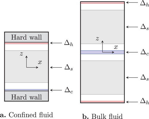
Table 1. Specification of simulation conditions. Exceptions are noted explicitly in the main text.

	A	H	N	$f_e$	$f_p$	${\mathrm{\Delta }}_c$	${\mathrm{\Delta }}_h$	${\mathrm{\Delta }}_s$
Confined fluids	100	5.5	800${}^{\mathrm{a}}$	0.5–40	–	$z\le -H+0.7$	$z\ge H-0.7$	$|z|\le H-2$
Bulk fluids	100	12	1920${}^{\mathrm{a}}$	0.5–40	0.5–80	$|z|\le 0.1$	$|z|\ge H-0.1$	$2\le |z|\le H-2$

Periodic boundary conditions were imposed in all three directions for bulk simulations, while the same conditions were imposed only in x- and y-directions for fluids in confinement.

Particles were placed randomly in the system and the system was equilibrated using Monte Carlo simulation first. To remove any overlap among particles, we replaced the hard sphere interaction by (22) $u(r)=\{\begin{array}{ll}{10}^9+1/r^{12}& \text{if }r\le 1,\\ 0& \mathrm{otherwise}.\end{array}$(22) A similar potential was used for interaction between particles and the walls. After we ensured the absence of overlap among particles and with the walls, we equilibrated the system further by MD. A single MD step consists of three elements [35]: (1) Search for the next pair of colliding particles, (2) advance the time and positions of all particles till the collision occurs, (3) assign the post-collision velocity vectors to the colliding particles, which are obtained from conservation laws of energy and momentum. For fluids in confinement, a minor modification was made to include an elastic collision with the hard walls.

A temperature gradient was imposed using RNEMD method [31], which was developed originally to compute viscosity and thermal conductivity. In this method, we choose two thin parallel swap regions ${\mathrm{\Delta }}_h$ and ${\mathrm{\Delta }}_c$ in the simulation box as illustrated in Figure 1(a ,b). The heating and cooling are achieved not through a contact with thermal baths, but by exchanging, with a fixed frequency $f_e$, the velocity vectors of a suitably chosen pair of particles: one with the lowest kinetic energy in ${\mathrm{\Delta }}_h$ and the other with the highest kinetic energy in ${\mathrm{\Delta }}_c$. We attempted a single swap move right after the step (3) described above with the probability given by the increment in time during step (2) multiplied by the set frequency $f_e$.

The swap move of RNEMD conserves the system energy exactly. Thus, even with the temperature gradient in the system, the total energy remains unaffected and $k_{\mathrm{B}}\overline{T}$ determined by Equation (21(21) $\sum _{i=1}^N\frac{1}{2}||{\mathbf{v}}_i|{|}^2=\frac{3}{2}(N-1)k_{\mathrm{B}}\overline{T},$(21) ) remains unity.

After a short MD run with the swap moves, the system reached a steady state and we sampled the density and the temperature profiles using the formulas given in Appendix 2. At least within the sampling regions ${\mathrm{\Delta }}_s$, which we chose to avoid the immediate vicinity of the swap regions, the temperature profile $k_{\mathrm{B}}{T}_{\mathrm{md}}$ from the simulation was well represented by a linear function (23) $k_{\mathrm{B}}{T}_{\mathrm{fit}1}(z)=a_{1}z+a_0$(23) for fluid in confinement and (24) $k_{\mathrm{B}}{T}_{\mathrm{fit}1}(z)=a_1|z|+a_0$(24) for a bulk fluid. We determined $a_0$ and $a_1$ by the least square fit to $k_{\mathrm{B}}{T}_{\mathrm{md}}$ within ${\mathrm{\Delta }}_s$. The resulting linear profile was extrapolated to all z values and used in Equation (16(16) $\lambda (z)=\lambda (0)-{\int }_{T(0)}^{T(z)}\frac{\chi }{\rho k_{\mathrm{B}}{T}^2}\mathrm{d}T,$(16) ) to generate the DDFT prediction of the density profile.

Equation (16(16) $\lambda (z)=\lambda (0)-{\int }_{T(0)}^{T(z)}\frac{\chi }{\rho k_{\mathrm{B}}{T}^2}\mathrm{d}T,$(16) ) is a consequence only of the local equilibrium assumption and $\mathrm{\nabla }p\equiv \mathbf{0}$. It follows that it remains valid even in the presence of a convective flow that does not involve a pressure gradient. To see if this is the case, we considered another type of RNEMD swap move in place of the energy swap move described above. In this case, the x-component $v_x$ of the velocity vector was swapped with frequency $f_p$ between a pair of particles: one in ${\mathrm{\Delta }}_c$ with the largest $v_x$ and the other in ${\mathrm{\Delta }}_h$ with the smallest (i.e. closest to $-\mathrm{\infty }$) $v_x$, resulting in a linear velocity profile ($v_x\propto z$).

This RNEMD move conserves both total energy and linear momentum of the system. However, since it generates a convective motion from the thermal fluctuation of particles, it leads to a loss of thermal energy in the swap regions. As a consequence, a non-uniform temperature field develops with its maximum located in ${\mathrm{\Delta }}_s$, causing the heat to flow into the swap regions, where it is converted into the convective motion. Because the energy associated with this motion dissipates into thermal energy throughout the system, a non-isothermal steady-state is maintained [31].

Finally, we note that the width of swap regions used in this work (0.2 as shown in Table 1) is much smaller than in typical RNEMD. Our choice leads to much more drastic temperature variations near the swap regions, and hence provides a more stringent test for our approach, which invokes local equilibrium assumption.

5. Results

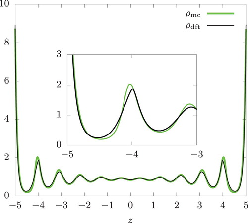
Let us consider hard spheres in confinement first. In Figures 2 and 3, we show density profiles from Monte Carlo simulation (${\rho }_{\mathrm{mc}}$) and isothermal DFT (${\rho }_{\mathrm{dft}}$), to which DDFT reduces if the temperature is uniform throughout the system. Two overall density values, n = 0.87 and 0.95, were selected since ${\rho }_{\mathrm{mc}}$ near the walls (z<−3) are very similar to those observed in MD (${\rho }_{\mathrm{md}}$) to be presented below but at n = 0.8 and with a temperature gradient. Except in $|z|>3$, the DFT predictions are in excellent agreement with the simulation. The discrepancy we do see for $|z|>3$ is larger for larger n.

Figure 2. Density profiles of a hard-sphere fluid between two parallel hard walls at $|z|=5.5$. From an isothermal Monte Carlo simulation (${\rho }_{\mathrm{mc}}$) and an isothermal DFT calculation (${\rho }_{\mathrm{dft}}$) at $k_{\mathrm{B}}\overline{T}=1$. The system contains N = 870 particles resulting in the overall density n = 0.87 (based on the volume accessible to the centres of the spheres). The inset provides an expanded view of the profiles near z = −5.

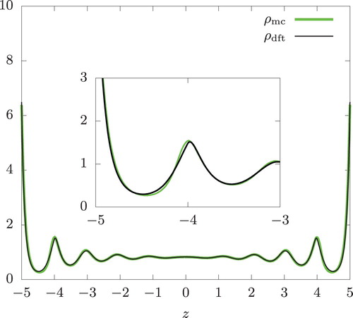
Figure 3. Same as Figure 2 but with N = 950 and n = 0.95. $k_{\mathrm{B}}\overline{T}=1$.

Next, we introduced the energy exchange RNEMD moves. The temperature gradient $\mathrm{d}{k}_{\mathrm{B}}{T}_{\mathrm{md}}/\mathrm{d}z$ was 0.0613 and 0.123 for the swap rates $f_e=10$ and 40, respectively. In other words, the temperature changes involved are 6 to 12 per cent of $k_{\mathrm{B}}\overline{T}$ within a distance of a single hard-sphere diameter. This is by no means small.

From Figures 4 and 5, we see a small discrepancy between ${\rho }_{\mathrm{md}}$ and the DDFT prediction (${\rho }_{\mathrm{ddft}}$) for z<−3 at these swap rates. At $f_e=40$, ${\rho }_{\mathrm{ddft}}$ in z<−4.2 shows a somewhat larger deviation than the corresponding portion in the isothermal system in Figure 3. Aside from this, the discrepancy between ${\rho }_{\mathrm{md}}$ and ${\rho }_{\mathrm{ddft}}$ is similar in magnitude to what we saw in the isothermal systems having similar density values in this region. Thus, very little inaccuracy was incurred when these highly non-isothermal systems are described by assuming local equilibrium.

Figure 4. Density and temperature profiles of a hard-sphere fluid between two parallel hard walls at $|z|=5.5$. From a RNEMD simulation (${\rho }_{\mathrm{md}}$ and $k_{\mathrm{B}}{T}_{\mathrm{md}}$) and DDFT calculation (${\rho }_{\mathrm{ddft}}$). The swap frequency $f_e=10$, the overall temperature $k_{\mathrm{B}}\overline{T}=1$, and the overall density n = 0.8. The inset provides an expanded view of the density profiles near z = −5.

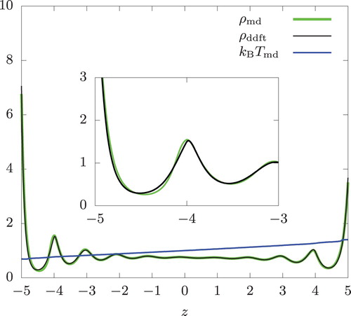
Figure 5. Same as Figure 4 but with $f_e=40$. $k_{\mathrm{B}}\overline{T}=1$ and n = 0.8.

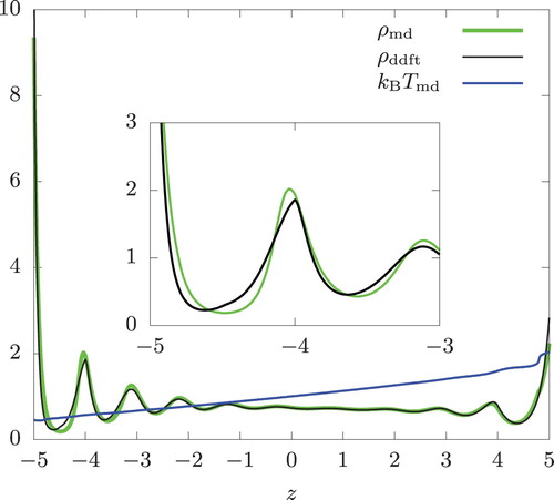
As expected, the fluid density is higher in the lower temperature region. With increasing $f_e$, the temperature decreases in the left half (z<0) of the system. Simultaneously, the discrepancy we are discussing is seen to grow. In contrast, ${\rho }_{\mathrm{ddft}}$ is in good agreement with ${\rho }_{\mathrm{md}}$ in the right half (z>0) of the system except at the immediate vicinity of the wall, where one of the swap region is located and the actual temperature ($k_{\mathrm{B}}{T}_{\mathrm{md}}$) is noticeably larger than $k_{\mathrm{B}}{T}_{\mathrm{fit}1}$. For swap rates smaller than 10, ${\rho }_{\mathrm{md}}$ and ${\rho }_{\mathrm{ddft}}$ were nearly indistinguishable.

The results for bulk simulations are shown in Figures 6 and 7. Since the system is symmetric about the xy-plane, ${\rho }_{\mathrm{md}}(z)$ and $k_{\mathrm{B}}{T}_{\mathrm{md}}(z)$ in these figures actually represent the arithmetic means of the data obtained from the simulations, i.e. $({\rho }_{\mathrm{md}}(-z)+{\rho }_{\mathrm{md}}(z))/2$ and $(k_{\mathrm{B}}{T}_{\mathrm{md}}(-z)+k_{\mathrm{B}}{T}_{\mathrm{md}}(z))/2$, respectively. The same remark applies to Figures 12 and 13.

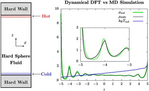
Figure 6. Density and temperature profiles of a bulk hard-sphere fluid. The swap frequency $f_e=10$, the overall temperature $k_{\mathrm{B}}\overline{T}=1$, and the overall density n = 0.8.

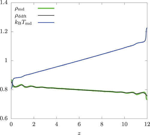
Figure 7. Same as Figure 7 but with $f_e=40$. $k_{\mathrm{B}}\overline{T}=1$ and n = 0.8.

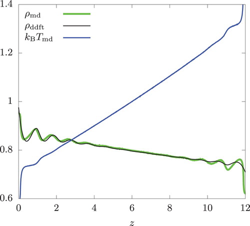
The temperature gradient $\mathrm{d}{k}_{\mathrm{B}}T/\mathrm{d}z$ was 0.0216 and 0.0514 for $f_e=10$ and 40, respectively. Interestingly, we observe a noticeable oscillation in the density profile, indicating layering of particles along the planes perpendicular to the heat flux. This is observed in both simulation and in the DDFT calculation. These two methods are in very good agreement except near z = 0 and 12, where the swap regions are located and $k_{\mathrm{B}}{T}_{\mathrm{md}}$ shows a large deviation from $k_{\mathrm{B}}{T}_{\mathrm{fit}1}$ assumed in the DDFT calculation.

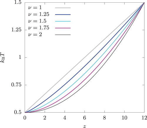
We emphasise that these oscillatory profiles are found in a bulk fluid without any walls. Because of the swap regions in the case of RNEMD and the imposed non-uniform temperature profile in the case of DDFT, our bulk system has lost the translational invariance in the z-direction. Thus, the observed behaviour is consistent with the symmetry principle. To understand the origin of this behaviour beyond this general observation, we considered the temperature profile of the form (25) $T(z)=T_0+(T_h-T_0){\left|\frac{z}{H}\right|}^{\nu },(|z|\le H)$(25) in additional DDFT calculations, where we set $k_{\mathrm{B}}{T}_0=0.5$ and $k_{\mathrm{B}}{T}_h=1.5$. This assumed temperature profile is shown in Figure 8 for several values of ν. Beyond $|z|=H$, the system is subject to the periodic boundary condition in the z-direction. Under the assumption of constant κ, only the linear temperature profile is physically sensible at a steady state. Nevertheless, the corresponding density profile can be found for other temperature profiles using Equation (16(16) $\lambda (z)=\lambda (0)-{\int }_{T(0)}^{T(z)}\frac{\chi }{\rho k_{\mathrm{B}}{T}^2}\mathrm{d}T,$(16) ) since, as mentioned earlier, its validity is based only on the assumptions that $\mathrm{\nabla }p\equiv \mathbf{0}$ and that the local equilibrium prevails.

Figure 8. The temperature profiles across a bulk system as given by Equation (25(25) $T(z)=T_0+(T_h-T_0){\left|\frac{z}{H}\right|}^{\nu },(|z|\le H)$(25) ). The periodic boundary condition is imposed to determine the profile beyond $|z|=12$.

The result of this set of calculation is shown in Figure 9. The oscillatory behaviour is observed near z = 0 for all ν values except $\nu =2$. At z = 0, $\mathrm{d}T/\mathrm{d}z$ and ${\mathrm{d}}^{2}T/\mathrm{d}{z}^2$ are discontinuous for $\nu =1$ and for $1<\nu <2$, respectively. The amplitude of oscillation near z = 0 is seen to decrease with increasing ν and the oscillation disappears completely at $\nu =2$. Under the periodic boundary condition, $\mathrm{d}T/\mathrm{d}z$ is discontinuous at $z=\pm H$ irrespective of the value of ν and the oscillatory density profile is observed near $|z|=H$ for all ν.

Figure 9. The density profiles corresponding to the temperature profiles shown in Figure 8. DDFT calculation.

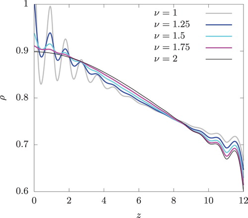
In DDFT, the oscillatory density profile arises only from the imposed temperature profile and the assumption of local equilibrium. This strongly indicates that the same behaviour observed in RNEMD simulation is not some artefact of the swap moves, which interfere with the natural evolution of the system governed by Newton's equations of motion. Instead, it is a physical response of the system to the temperature profile generated by the RNEMD moves.

One possible scenario that can lead to the observed layering of particles is as follows. Since the density is higher in the lower temperature region, the particles tend to accumulate near z = 0. For a smooth temperature profile, fluctuations that displace these particles leave the temperature surrounding them relatively unaffected. For less smooth profiles, this is not the case, thus requiring a larger density change. As a result, the accumulation of particles may be sufficiently persistent and this prevents other particles from occupying the nearby space. On the other hand, particles near z = 12, having larger kinetic energies, may also serve to repel other particles from this region.

For the purpose of determining κ by RNEMD, the observed oscillatory density profile is undesirable. However, the issue can be minimised by using a smaller $f_e$ or a larger width for the swap regions.

Within and near the swap regions of RNEMD, a discrepancy of varying degree exists between $k_{\mathrm{B}}{T}_{\mathrm{md}}$ and $k_{\mathrm{B}}{T}_{\mathrm{fit}1}$. To see how this discrepancy impacts the DDFT predictions, we used $k_{\mathrm{B}}{T}_{\mathrm{md}}$ directly in Equation (16(16) $\lambda (z)=\lambda (0)-{\int }_{T(0)}^{T(z)}\frac{\chi }{\rho k_{\mathrm{B}}{T}^2}\mathrm{d}T,$(16) ).

In the case of confined fluids (corresponding to the results shown in Figures 4 and 5), this did not noticeably affect the predicted density profiles away from the walls. As seen from Figure 10, the prediction improved markedly in the vicinity of the cold wall but only between $z\approx -4.95\sim -4.85$. (Below $z\approx -4.95$, ${\rho }_{\mathrm{md}}$ was between two DDFT predictions, but somewhat closer to ${\rho }_{\mathrm{ddft}}$ obtained with $k_{\mathrm{B}}{T}_{\mathrm{md}}$.) The accuracy worsened somewhat at around $z\approx -4$. The situation on the hot wall is also mixed. We see from Figure 11 that the density at contact (z = 5) is more accurately predicted when $k_{\mathrm{B}}{T}_{\mathrm{md}}$ is used directly. The density profile also captures a small decrease in $\mathrm{d}\rho /\mathrm{d}z$ due to the sudden increase in temperature at the edge of the swap region (at z = 4.8, where $\mathrm{d}{k}_{\mathrm{B}}{T}_{\mathrm{md}}/\mathrm{d}z=5.0$ for $f_e=40$). However, DDFT is seen to over-predict the change in $\mathrm{d}\rho /\mathrm{d}z$ and, as a result, its prediction away from the wall deviates from ${\rho }_{\mathrm{md}}$, with the latter nearly perfectly interpolating the two separate DDFT predictions.

Figure 10. Density and temperature profiles of a hard-sphere fluid near the cold wall. Swap frequency $f_e=40$, the overall temperature $k_{\mathrm{B}}\overline{T}=1$, and the overall density n = 0.8.

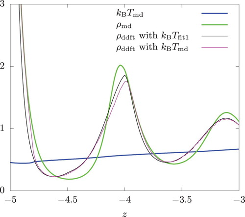
Figure 11. Density and temperature profiles of a hard-sphere fluid near the hot wall. Swap frequency $f_e=40$, the overall temperature $k_{\mathrm{B}}\overline{T}=1$, and overall density n = 0.8.

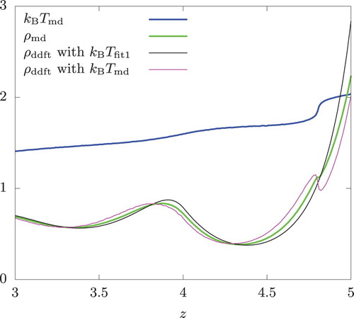
Figure 12. The temperature profiles across a bulk system with momentum exchanging RNEMD moves. The swap frequency $f_p=80$, the apparent overall temperature $k_{\mathrm{B}}{\overline{T}}^{\mathrm{app}}=1$, and the overall density n = 0.8.

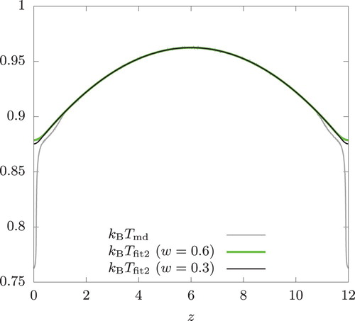
Figure 13. A comparison of density profiles corresponding to the temperature profiles shown in Figure 12.

In the case of bulk fluids (corresponding to the results in Figures 6 and 7), however, the DDFT prediction was much worse when $k_{\mathrm{B}}{T}_{\mathrm{md}}$ was used directly and showed an oscillatory profile with much larger amplitudes than were observed in simulations. In the energy exchange RNEMD, a sharp temperature change occurs at each edge of the swap regions. The largest temperature gradient observed at these edges was 1.8 for $f_e=10$ and 6.6 for $f_e=40$. As a result, $k_{\mathrm{B}}{T}_{\mathrm{md}}$ acquires a very narrow peak or valley within a distance of 0.2 (the thickness of the swap regions in this study), and this leads to the considerable over-prediction by DDFT. In fact, the amplitude of oscillation decreased significantly when the width of the sampling regions was increased to 1.

Introducing the momentum exchange move of RNEMD, we also examined the effect of a shear flow, but focusing only on the bulk system. The frequency $f_p$ for the momentum exchange move was set to 80, resulting in the velocity gradient $\mathrm{d}{v}_x/\mathrm{d}z=0.133$ . The apparent temperature $k_{\mathrm{B}}{\overline{T}}^{\mathrm{app}}$, as given by Equation (A14(A14) $\frac{3}{2}(N-1)k_{\mathrm{B}}{\overline{T}}^{\mathrm{app}}:=\frac{1}{2}\sum _i||{\mathbf{v}}_i|{|}^2$(A14) ), was set to unity. Smaller $f_p$ values were also examined, but they do not alter the conclusion to be presented below.

As already mentioned, this RNEMD move also induces a temperature variation in the system. The resulting temperature profile $k_{\mathrm{B}}{T}_{\mathrm{md}}$ was computed using Equations (A16(A16) $k_{\mathrm{B}}{T}_a=k_{\mathrm{B}}{T}_a^{\mathrm{app}}-\frac{N}{3(N-1)}{u_a}^2,$(A16) ) and (A17(A17) $k_{\mathrm{B}}{T}_a^{\mathrm{app}}:=\frac{N}{3(N-1)}\frac{1}{⟨N_a⟩}⟨\sum _{i\in a}||{\mathbf{v}}_i|{|}^2⟩.$(A17) ), and is shown in Figure 12.

Within the sampling region ${\mathrm{\Delta }}_s$, $k_{\mathrm{B}}{T}_{\mathrm{md}}$ is well described by a quadratic function centred around $|z|=H/2$. However, $k_{\mathrm{B}}{T}_{\mathrm{md}}$ exhibits a very sharp decrease near $|z|=0$ and H. We recall that $k_{\mathrm{B}}{T}_{\mathrm{md}}$ is symmetric around z = 0 and repeats itself under the periodic boundary conditions. To suppress the over-prediction of the oscillatory behaviour, we replaced this rapidly changing portion of the temperature profile by a quartic equation in our DDFT calculation. That is, we represent $k_{\mathrm{B}}{T}_{\mathrm{md}}$ by (26) $\begin{array}{rl}& k_{\mathrm{B}}{T}_{\mathrm{fit}2}\\ & =\{\begin{array}{ll}{b}_4|z{|}^4+b_2|z{|}^2+b_0,& \text{if }z\in {\mathrm{\Delta }}_c^w,\\ b_4(H-|z|{)}^4+b_2(H-|z|{)}^2+b_0,& \text{if }z\in {\mathrm{\Delta }}_h^w,\\ -c_2(|z|-H/2{)}^2+c_0,& \mathrm{otherwise},\end{array}\end{array}$(26) where ${\mathrm{\Delta }}_c^w$ and ${\mathrm{\Delta }}_h^w$ are defined by $|z|\le w$ and $|z|>H-w$, respectively. We determined $c_0$ and $c_2$ by fitting the quadratic equation to $k_{\mathrm{B}}{T}_{\mathrm{md}}$ in ${\mathrm{\Delta }}_s$, while $b_0$, $b_2$, and $b_4$ were determined to ensure continuity of $k_{\mathrm{B}}{T}_{\mathrm{fit}2}$ and its first and second derivatives at $|z|=w$.

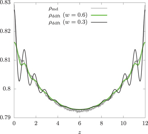
As seen from Figure 13, ${\rho }_{\mathrm{ddft}}$ is in good agreement with ${\rho }_{\mathrm{md}}$. The DDFT prediction can be improved if $c_0$ and $c_2$ are determined using $k_{\mathrm{B}}{T}_{\mathrm{md}}$ from a wider range of z to better represent it near the swap regions. Thus, our approach to supplement DDFT with the local equilibrium assumption remains applicable even in the presence of a shear flow provided that the temperature profile is accurately represented and it has no sharp peak or valley. Consistent with the observation made above, ${\rho }_{\mathrm{ddft}}$ develops the oscillatory behaviour as valleys of $k_{\mathrm{B}}{T}_{\mathrm{fit}2}$ (at $|z|=0$ and 12) becomes sharper with decreasing w.

6. Concluding remarks

Using a version of DDFT, we explored microstructure of non-isothermal hard-sphere fluids both in confinement and in bulk. Combined with the assumption of local equilibrium, the entropy functional developed in  [26] led to predictions of the density profiles in very good overall agreement with the simulation results, in which a temperature gradient was created by the RNEMD method.

In formulating DDFT, Anero et al. [26] did not include velocity field in the set of relevant variables, thus focusing on systems without a convective motion. Nevertheless, we showed that their DDFT can be used to predict density profile in the presence of a shear flow at least in the case of a one-dimensional steady-state problem in rectangular coordinates provided that the pressure gradient is zero throughout the system.

Because RNEMD depends on the availability of a suitable pair of particles in the swap regions, there is a limit to the temperature gradient that can be achieved. While a larger temperature gradient can be generated using thicker swap regions, the temperature gradient we considered in this work was by no means trivial, in some cases, leading to the temperature variation comparable to the overall system temperature itself within the distance of 10 times the hard sphere diameter.

Interestingly, the energy exchanging RNEMD moves induces an oscillatory density profile even in bulk, and this behaviour was predicted correctly by our approach. However, DDFT over-predicts the amplitude of oscillation if the temperature exhibits a sharp change over a very small distance. This may point to a breakdown of the local equilibrium assumption under such extreme conditions.

Acknowledgements

Computations reported here were made possible by a resource grant from the Ohio Supercomputer Center [36].

Disclosure statement

No potential conflict of interest was reported by the author(s).

Additional information

Funding

Computations reported here were made possible by a resource grant from the Ohio Supercomputer Center.

Notes

${}^a$This gives overall density n = 0.8 based on the volume accessible to the centres of hard spheres.

Appendices

Appendix 1. Key formulas from fundamental measure theory

In this appendix, we summarise the key results of Rosenfeld's fundamental measure theory from  [32,33], which gives Φ as a function of three weighted densities. In one-dimensional problems (of a three-dimensional system and in rectangular coordinates), they are given by [34] (A1) ${\rho }_k(z):=\frac{1}{2{\sigma }^{k+1}}{\int }_{-\sigma }^{\sigma }\rho (z+\zeta ){\zeta }^k\mathrm{d}\zeta (k=0,1,2).$(A1) Then, (A2) $\mathrm{\Phi }=\sum _{i=1}^3{\varphi }_i({\rho }_0,{\rho }_1,{\rho }_2),$(A2) in which (A3) $\begin{array}{rl}{\varphi }_0& =-{\rho }_0\ln (1-\eta ),\end{array}$(A3) (A4) $\begin{array}{rl}{\varphi }_1& =4\pi {\sigma }^3\frac{{{\rho }_0}^2-{{\rho }_1}^2}{1-\eta },\end{array}$(A4) (A5) $\begin{array}{rl}{\varphi }_2& =3{\pi }^2{\sigma }^6\frac{({\rho }_0-{\rho }_2)({{\rho }_0}^2-4{{\rho }_1}^2+3{{\rho }_2}^2)}{(1-\eta {)}^2},\end{array}$(A5) and (A6) $\eta =2\pi {\sigma }^3({\rho }_0-{\rho }_2).$(A6) The functional derivative involved in the expressions for λ and $\beta \chi$ can now be evaluated: (A7) $\frac{\delta }{\delta \rho (z)}\int \mathrm{\Phi }[\rho ;z)\mathrm{d}z=\sum _{k=0}^2\frac{1}{2{\sigma }^{k+1}}{\int }_{-\sigma }^{\sigma }{\frac{\mathrm{\partial }\mathrm{\Phi }}{\mathrm{\partial }{\rho }_k}|}_{z-\zeta }{\zeta }^k\mathrm{d}\zeta .$(A7)

Appendix 2. Temperature and convection

In this appendix, we list several key equations pertaining to profiles of density, temperature, and velocity. Corrections to the overall system temperature and the temperature field due to a convective motion will also be considered. As in the main text, m = 1 and no explicit reference will be made to m.

Let $\mathbf{u}(z)=u(z){\mathbf{e}}_x$ be the velocity profile of the convective motion in the system, where ${\mathbf{e}}_x$ is the unit vector pointing in the positive x-direction. Needless to say, $u(z)$ cannot be determined as a continuous function of z in simulation. Instead, we slice the system into thin layers of thickness δ in the direction perpendicular to the z-axis. In this work, we set $\delta =0.01$. Using a to label the layers, we define the density and the velocity profiles by (A8) $\rho (z)={\rho }_{a(z)}:=\frac{1}{A\delta }⟨N_a⟩$(A8) and (A9) $u(z)=u_{a(z)}:=\frac{1}{⟨N_a⟩}⟨\sum _{i\in a}{v}_{ix}⟩,$(A9) respectively, where $a(z)$ refers to the layer containing the position z, $N_a$ is the instantaneous number of particles in this layer, and $v_{ix}$ is the x-component of the velocity vector ${\mathbf{v}}_i$ of particle i. As indicated by $i\in a$, the sum is only over the ath layer.

Subtracting the contribution from the bulk motion, we define the overall system temperature $k_{\mathrm{B}}\overline{T}$ by (A10) $\begin{array}{rl}\frac{3}{2}(N-1)k_{\mathrm{B}}\overline{T}& =\frac{1}{2}⟨\sum _{i=1}^N||{\mathbf{v}}_i-\mathbf{u}(z_i)|{|}^2⟩\\ & =\frac{1}{2}⟨\sum _{i=1}^N[||{\mathbf{v}}_i|{|}^2-2u_i{v}_{ix}+{u_i}^2]⟩\end{array}$(A10) where $u_i:=u_{a(z_i)}$.

We can carry out the sum over all particles i in the system in two steps, summing over particles in the ath layer first and summing over all layers next. This gives (A11) $\sum _i{u}_i{v}_{ix}=\sum _a\sum _{i\in a}{u}_i{v}_{ix}=\sum _a{u}_a\sum _{i\in a}{v}_{ix}.$(A11) Upon averaging, (A12) $⟨\sum _i{u}_i{v}_{ix}⟩=\sum _a{u}_a⟨\sum _{i\in a}{v}_{ix}⟩=\sum _a{\rho }_a{u_a}^{2}A\delta .$(A12) A similar process for $\sum _i{u_i}^2$ leads to the identical result. Thus, (A13) $\frac{3}{2}(N-1)k_{\mathrm{B}}\overline{T}=\frac{3}{2}(N-1)k_{\mathrm{B}}{\overline{T}}^{\mathrm{app}}-\frac{1}{2}\sum _a{\rho }_a{u_a}^{2}A\delta ,$(A13) where (A14) $\frac{3}{2}(N-1)k_{\mathrm{B}}{\overline{T}}^{\mathrm{app}}:=\frac{1}{2}\sum _i||{\mathbf{v}}_i|{|}^2$(A14)

defines the apparent overall system temperature. We dropped the time averaging $⟨\cdot ⟩$ since the molecular dynamics of hard spheres conserves the total kinetic energy. The second term of Equation (A13(A13) $\frac{3}{2}(N-1)k_{\mathrm{B}}\overline{T}=\frac{3}{2}(N-1)k_{\mathrm{B}}{\overline{T}}^{\mathrm{app}}-\frac{1}{2}\sum _a{\rho }_a{u_a}^{2}A\delta ,$(A13) ) is the correction due to the convective motion.

We now define the temperature profile by (A15) $k_{\mathrm{B}}T(z)=k_{\mathrm{B}}{T}_{a(z)}:=\frac{N}{3(N-1)}\frac{1}{⟨N_a⟩}⟨\sum _{i\in a}||{\mathbf{v}}_i-\mathbf{u}(z_i)|{|}^2⟩.$(A15) For a reasonably large system, the factor $N/(N-1)$ is very nearly equal to unity and it can be omitted. Proceeding as before, we arrive at (A16) $k_{\mathrm{B}}{T}_a=k_{\mathrm{B}}{T}_a^{\mathrm{app}}-\frac{N}{3(N-1)}{u_a}^2,$(A16) in which (A17) $k_{\mathrm{B}}{T}_a^{\mathrm{app}}:=\frac{N}{3(N-1)}\frac{1}{⟨N_a⟩}⟨\sum _{i\in a}||{\mathbf{v}}_i|{|}^2⟩.$(A17) If $u_a\equiv 0$ for all a, then $k_{\mathrm{B}}{T}_a=k_{\mathrm{B}}{T}_a^{\mathrm{app}}$. If in addition $k_{\mathrm{B}}{T}_a=k_{\mathrm{B}}\overline{T}$, a constant independent of a, Equation (A17(A17) $k_{\mathrm{B}}{T}_a^{\mathrm{app}}:=\frac{N}{3(N-1)}\frac{1}{⟨N_a⟩}⟨\sum _{i\in a}||{\mathbf{v}}_i|{|}^2⟩.$(A17) ) reduces to (A18) $\frac{3}{2}(N-1)⟨N_a⟩k_{\mathrm{B}}\overline{T}=\frac{N}{2}⟨\sum _{i\in a}||{\mathbf{v}}_i|{|}^2⟩.$(A18) Upon summation over all layers a, we recover Equation (21(21) $\sum _{i=1}^N\frac{1}{2}||{\mathbf{v}}_i|{|}^2=\frac{3}{2}(N-1)k_{\mathrm{B}}\overline{T},$(21) ). This points to the need for the $N/(N-1)$ factor at least in principle, if not in practice.

References

- R. Evans, Adv. Phys. 28, 143 (1979). doi:10.1080/00018737900101365
- L.D. Gelb, K.E. Gubbins, R. Radhakrishnan and M. Sliwinska-Bartkowiak, Rep. Prog. Phys. 62, 1573 (1999). doi:10.1088/0034-4885/62/12/201
- D.W. Oxtoby, in Fundamentals of Inhomogeneous Fluids, edited by D. Henderson (Marcel Dekker, New York, NY, 1992), pp. 407–442.
- V. Talanquer and D.W. Oxtoby, J. Chem. Phys. 100, 5190 (1994). doi:10.1063/1.467183
- D.S. Dean, J. Phys. A: Math. Gen. 29, L613 (1996). doi:10.1088/0305-4470/29/24/001
- U. Marini Bettolo Marconi and P. Tarazona, J. Chem. Phys. 110, 8032 (1999). doi:10.1063/1.478705
- H.T. Davis, J. Chem. Phys 86, 1474 (1987). doi:10.1063/1.452237
- L.A. Pozhar and K.E. Gubbins, J. Chem. Phys. 99, 8970 (1993). doi:10.1063/1.465567
- A.J. Archer, J. Phys.: Condens. Matter 18, 5617 (2006).
- Z. Guo, T.S. Zhao and Y. Shi, Phys. Fluids 18, 067107 (2006). doi:10.1063/1.2214367
- J.G. Anero and P. Español, Europhys. Lett. 78, 50005 (2007). doi:10.1209/0295-5075/78/50005
- U. Marini Bettolo Marconi, P.T.F. Cecconi and S. Melchionna, J. Phys. Condens. Matter 20, 494233 (2008). doi:10.1088/0953-8984/20/49/494233
- A.J. Archer, J. Chem. Phys. 130, 014509 (2009). doi:10.1063/1.3054633
- U. Marini Bettolo Marconi and S. Melchionna, J. Phys. Condens. Matter 22, 364110 (2010). doi:10.1088/0953-8984/22/36/364110
- B.D. Goddard, A. Nold, N. Savva, P. Yatsyshin and S. Kalliadasis, J. Phys.: Condns. Matt. 25, 035101 (2013).
- U. Marini Bettolo Marconi and S. Melchionna, Commun. Theor. Phys. 62, 596 (2014). doi:10.1088/0253-6102/62/4/17
- E.S. Kikkinides and P.A. Monson, J. Chem. Phys. 142, 094706 (2015). doi:10.1063/1.4913636
- J.-P. Hansen and I.R. McDonald, Theory of Simple Liquids: With Applications to Soft Matter, 4th ed. (Academic Press, Oxford, 2013).
- J.H. Irving and J.G. Kirkwood, J. Chem. Phys. 18, 817 (1950). doi:10.1063/1.1747782
- H. van Beijeren and M.H. Ernst, Physica 68, 437 (1973). doi:10.1016/0031-8914(73)90372-8
- J.W. Dufty, A. Santos and J.J. Brey, Phys. Rev. Lett. 77, 1270 (1996). doi:10.1103/PhysRevLett.77.1270
- A. Santos, J.M. Montanero, J.W. Dufty and J.J. Brey, Phys. Rev. E 57, 1644 (1998). doi:10.1103/PhysRevE.57.1644
- S. Harris, An Introduction to the Theory of the Boltzmann Equation (Dover, New York, NY, 2004).
- P. Español and H. Löwen, J. Chem. Phys. 131, 244101 (2009). doi:10.1063/1.3266943
- R. Wittkowski, H. Löwen and H.R. Brand, J. Chem. Phys. 137, 224904 (2012). doi:10.1063/1.4769101
- J.G. Anero, P. Español and P. Tarazona, J. Chem. Phys. 139, 034106 (2013). doi:10.1063/1.4811655
- H. Grabert, Projection Operator Techniques in Nonequilibrium Statistical Mechanics (Springer, Berlin, 1982).
- E.T. Jaynes, Phys. Rev. 106, 620 (1957). doi:10.1103/PhysRev.106.620
- S. Whitaker, Introduction to Fluid Mechanics (Krieger Publishing Company, Florida, 1992).
- S. Whitaker, Fundamental Principles of Heat Transfer (Krieger Publishing Company, Florida, 1983).
- F. Müller-Plathe and P. Bordat, in Novel Methods in Soft Matter Simulation, Lecture Notes in Physics 640, edited by M. Karttunen, I. Vattulainen, and A. Lukkarinen (Springer, Berlin, Heidelberg, 2004), pp. 310–326.
- Y. Rosenfeld, Phys. Rev. Lett. 63, 980 (1989). doi:10.1103/PhysRevLett.63.980
- P. Tarazona, Phys. Rev. Lett. 84, 694 (2000). doi:10.1103/PhysRevLett.84.694
- P. Tarazona, J.A. Cuesta and Y. Martínes-Ratón, in Theory and Simulation of Hard-Sphere Fluids and Related Systems, edited by A. Mulero (Springer-Verlag, Berlin, Heidelberg, 2008), pp. 247–341.
- M.P. Allen and D.J. Tildesley, Computer Simulation of Liquids (Oxford University Press, New York, NY, 1987).
- Ohio Supercomputer Center, Ohio supercomputer center (1987). http://osc.edu/ark:/19495/f5s1ph73