Continuum model of the simple dielectric fluid: consistency between density based and continuum mechanics methods

ABSTRACT

The basic continuum model for polar fluids is deceptively simple. The free energy integral consists of four terms: the coupling of polarisation to an external field, the electrostatic energy of the induced electric field interacting with itself and the stored polarisation energy quadratic in the polarisation. A local function of density accounts for the mechanical state of the fluid. Viewed as a non-equilibrium free energy functional of number density and polarisation, minimisation in these two densities under constraints of the Maxwell field equations should lead to the correct equilibrium state. The alternative is a continuum mechanics approach in which the mechanical degree of freedom is extended to full deformation. We show that the continuum electromechanics method leads to a force balance equation which is consistent with the density functional equilibrium equation. The continuum mechanics procedure is significantly more demanding. The gain is a well-defined pressure tensor derived from deformation of total energy. This resolves the issue of the uncertainty in the pressure tensor obtained from integration of the force density, which is the conventional method in density based thermomechanics. Our derivation is based on the variational electrostatics approach developed by Ericksen (Arch. Rational Mech. Anal. 183 299 (2007)).

GRAPHICAL ABSTRACT

Keywords:

• Simple dielectric fluid
• electromechanics
• Maxwell stress tensor
• Kelvin forces
• electrostriction

1. Introduction

Free energy functionals for polarisation fluctuations were introduced by Marcus to account for non-equilibrium solvation driving electron transfer in polar solvents [1,2]. Non-equilibrium polarisation functionals in the more recent literature are often referred to as Marcus–Felderhof functionals, adding the name of Felderhof who carried out a systematic study of their properties and foundation in linear response theory [3,4]. Non-equilibrium polarisation continues to play an important role in the theory of reaction dynamics in polar solvents [5] (for a recent review, see Dinpajooh et al. [6]).

The Marcus–Felderhof functional also found application in equilibrium continuum theory as it can be used for variational determination of polarisation in a dielectric medium interacting with fixed charge distributions [6–9]. Computation of equilibrium polarisation in complex geometries indeed is a major challenge. The long range nature of the dipolar tensor makes direct minimisation of polarisation cumbersome and expensive [10]. Improving the efficiency and numerical stability of these calculations has become a focus of research relevant for a large variety of applications such as colloidal and interface science, electrochemistry and biophysics. One option popular in physical chemistry is to turn the integration of the electrostatic interactions into a boundary value problem optimising the polarisation surface charges instead of the volume polarisation [10–13].

While the representation of polarisation in terms of surface and interface charges is mathematically valid and physically meaningful [14], an alternative is to exploit the power (and inspiring elegance) of Maxwell theory and describe the long-range electrostatic interactions in terms of fields satisfying local differential equations. The idea would be to rewrite the non-local interaction between polarisation at different locations as an integral over the square of the local electric field generated by the polarisation (its longitudinal component [6,14]). The electric field is determined by solving the Maxwell equations converting the non-local integral equation to a set of coupled local (partial) differential equations [10,15]. The field equation for the Maxwell electric field requiring it to be curl free is readily satisfied by representing it as the gradient of a potential. That leaves the Maxwell equation for the dielectric displacement field providing the coupling to the polarisation and external charge. This approach amounts to a Maxwell field formulation of the Marcus–Felderhof functional.

Ideally one would like to treat the electric potential as an additional variational degree of freedom. Hopefully the corresponding Euler–Lagrange equation would be equivalent to the Maxwell equation for the dielectric field. This hope is frustrated by a curious complication. The proper field equation for dielectric displacement can only be recovered from a Legendre transform of the energy functional, which, unfortunately, changes the minimum to a saddle point which makes the procedure unsuitable as for application in numerical schemes [9,10]. A similar difficulty was encountered in the quest for a variational solution of the Poisson–Boltzmann equation for ionic solutions where the problem acquired a certain notoriety [15,16]. An ingenious solution proposed by Anthony Maggs is to impose the Maxwell equations by means of constraints implemented by the method of undetermined Lagrange multipliers [9].

Variational electrostatics is pursued in many diverse disciplines sometimes with little overlap. A development parallel to the activity in the physical chemistry of fluids took place in the field of continuum mechanics of solids [17,18]. Of particular interest is the approach of J. L. Ericksen who reconsidered the use of an extended variational scheme with the dielectric displacement as basis rather than the electric field [17]. The divergence of dielectric displacement (also called electric induction) vanishes in a dielectric continuum without embedded external charge and can therefore be represented as the curl of a vector potential, just as the magnetic induction. Using a convenient form of the energy functional Ericksen found that under conditions of stationarity for variation of this vector potential the curl of the electric field is zero, as required by the conjugate Maxwell equation [17]. Moreover, being an expression of the original Marcus–Felderhof functional in different variables, the energy functional remains convex. Even if somewhat exotic, the Ericksen scheme has definite advantages, certainly in formal derivations (see, e.g.  [19]). It is the method adopted here and will be explained in explicit mathematical detail in Section 3.

Ericksen developed his method as part of the continuing effort of merging electrostatics and elasticity theory. This research program stretching over more than 50 years was initiated by two seminal papers by Toupin [20,21] (for recent reviews, see e.g. [22–24]). The theoretical challenge in continuum electromechanics goes well beyond the problems faced in variational electrostatics of rigid systems. Now, in addition to the two Maxwell equations, a third field equation must be satisfied, namely force balance (the Cauchy equation). The central quantity in continuum mechanics is not force density but the stress tensor. The key question is therefore what is the appropriate stress tensor for electroelastic systems. As can be expected, this will be a combination of a form of the Maxwell stress tensor and mechanical stress due to short range (contact) interactions. However, this partition is not unique leading to different expression for total stress [23]. Toupin derived his electromechanical stress tensor applying the principle of virtual work (for a gentle introduction, we recommend [22]). Ericksen went back to this work trying to derive the Toupin stress using minimum energy methods [17].

Stress in linear elasticity theory is the work conjugate of strain. However, applications to soft matter, including elastic fluids, are based on non-linear elasticity theory originally developed for materials such as rubber. Elasticity theory for finite deformation is usually formulated in a Lagrangian framework [25]. This raises the question what is the Lagrangian (material) form of the electric field and dielectric displacement. This was resolved by Dorfmann and Ogden [26] building on earlier work on electro-acoustics by Lax and Nelson [27]. This is the methodology used in this paper. Lagrangian electromechanics is unfamiliar for most physical chemists with a statistical mechanics background. For this reason, after specifying the continuum model system in Section 2.1, we present in Section 2.2 our main result in the language of the classical density functional theory (DFT) of liquids. The following technical sections 4–7 fill in the rather heavy mathematical detail. We conclude in Section 8 with a discussion.

Summarising the aim of this work, the question we set out to answer is whether the differential equation for equilibrium density is consistent with the continuum mechanical equation for deformation of the model simple dielectric fluid considered. The reason that this might be in doubt is that the energy of polarised dielectric systems is sensitive to volume conserving (shear) deformations which are not accessed in an approach restricted to coupled density-polarisation variation. A lengthy derivation shows that this concern is not justified. The equilibrium density and polarisation solving the Euler Langrange equation for these variables are also solutions of the force balance equation of continuum mechanics (the electromechanical Cauchy equation). The centre piece in this argument is a systematic derivation of the dielectric stress tensor using the Langrangian electromechanical theory of Ref. [26] applied in the variational framework developed by Ericksen [17]. This yields an expression for the stress tensor in agreement with the one obtained by Ericksen using his own slightly different methodology. Bringing this particular dielectric stress tensor and its derivation to the attention of the physical chemistry community is the more practical aim of this investigation.

2. System definition and statement of main result

2.1. Free energy of the simple dielectric fluid

Taking density ρ and polarisation $\mathbf{p}$ as the primitive variables the continuum model of the simple dielectric fluid is specified by a functional (1) ${\mathcal{F}}_{\mathrm{d}}[\rho ,\mathbf{p}]={\mathcal{F}}_M[\rho ]+{\mathcal{F}}_P[\rho ,\mathbf{p}]+{\mathcal{E}}_F[\mathbf{p}]$(1) ${\mathcal{F}}_M$ defines the purely mechanical component of ${\mathcal{F}}_d$. (2) ${\mathcal{F}}_M[\rho ]={\mathcal{F}}_{sr}[\rho ]+{\int }_{\mathrm{\Omega }}{v}_{ext}(\mathbf{r})\rho (\mathbf{r})\mathrm{d}v$(2) ${\mathcal{F}}_{sr}$ describes the short range interactions. In a ‘simple’ fluid, it is the regular integral over a local free energy density $\varphi (\rho )$ (3) ${\mathcal{F}}_{sr}[\rho ]={\int }_{\mathrm{\Omega }}\varphi (\rho )\mathrm{d}v$(3) where Ω is the volume of the body of liquid ($dv=d^3\mathbf{r}$ is an infinitesimal volume element). The second term in Equation (2(2) ${\mathcal{F}}_M[\rho ]={\mathcal{F}}_{sr}[\rho ]+{\int }_{\mathrm{\Omega }}{v}_{ext}(\mathbf{r})\rho (\mathbf{r})\mathrm{d}v$(2) ) is the usual coupling to an external potential $v_{ext}$. Assuming linear dielectrics, ${\mathcal{F}}_P$ is the stored polarisation energy written as (4) ${\mathcal{F}}_P[\rho ,\mathbf{p}]={\int }_{\mathrm{\Omega }}\frac{{\mathbf{p}}^2}{2\chi (\rho )}\mathrm{d}v$(4) The susceptibility $\chi (\rho )$ is allowed to vary with density (electrostriction).

The last term in Equation (1(1) ${\mathcal{F}}_{\mathrm{d}}[\rho ,\mathbf{p}]={\mathcal{F}}_M[\rho ]+{\mathcal{F}}_P[\rho ,\mathbf{p}]+{\mathcal{E}}_F[\mathbf{p}]$(1) ) is the electrostatic energy ${\mathcal{E}}_F$. In the formulation of Refs. [3,8], the electrostatic energy consists of the coupling of the polarisation to the external field and an integral of the dipolar tensor coupling polarisation at different locations. This form of ${\mathcal{E}}_F$ stays close to particle based statistical mechanics and the density functional theory (DFT) of polar liquids. Ericksen, however, starts from the total electrostatic of energy Maxwell–Lorentz field theory [28] (5) ${\mathcal{E}}_F={\int }_V\frac{{ϵ}_0{\mathbf{e}}^2}{2}\mathrm{d}v$(5) where $\mathbf{e}$ is the Maxwell electric field and ${ϵ}_0$ the dielectric permittivity of vacuum. The energy ${\mathcal{E}}_F$ includes the electrostatic energy of the vacuum field. Separating this energy out we can write (6) ${\mathcal{E}}_F={\int }_V\frac{{ϵ}_0{\mathbf{e}}_0^2}{2}\mathrm{d}v+{\mathcal{U}}_F$(6) ${\mathcal{U}}_F$ plays the role of the system field energy which should vanish when the dielectric material is removed. The expression Ericksen uses for ${\mathcal{U}}_F$ is an integral over an energy density $e_{\mathrm{E}}$ (7) ${\mathcal{U}}_F={\int }_V{e}_{\mathrm{E}}(\mathbf{p})\mathrm{d}v\equiv {\mathcal{E}}_{\mathrm{E}}$(7) with $e_{\mathrm{E}}$ given by Ericksen [17] (8) $e_{\mathrm{E}}(\mathbf{p})=-\mathbf{p}\cdot {\mathbf{e}}_0+\frac{{ϵ}_0{\hat{\mathbf{e}}}^2}{2}$(8) where $\hat{\mathbf{e}}$ is response field. $\hat{\mathbf{e}}$ is related to the Maxwell field $\mathbf{e}$ and applied field ${\mathbf{e}}_0$ as (9) $\mathbf{e}={\mathbf{e}}_0+\hat{\mathbf{e}}$(9) $\hat{\mathbf{e}}$ is commonly referred to as the self field. (We have adopted the compact hat notation of Ref. [19] to distinguish between self field and Maxwell field.)

The internal electrostatic field energy density of Equation (8(8) $e_{\mathrm{E}}(\mathbf{p})=-\mathbf{p}\cdot {\mathbf{e}}_0+\frac{{ϵ}_0{\hat{\mathbf{e}}}^2}{2}$(8) ) is specific for finite body geometry. The dielectric occupying a finite volume Ω is enclosed in a container of total volume $V\gg \mathrm{\Omega }$ (vacuum when empty). While polarisation is confined to the body ($\mathbf{p}=0$ outside) the self field $\hat{\mathbf{e}}$ spills out and is nonzero in a region surrounding the body. That is why the integration in Equation (7(7) ${\mathcal{U}}_F={\int }_V{e}_{\mathrm{E}}(\mathbf{p})\mathrm{d}v\equiv {\mathcal{E}}_{\mathrm{E}}$(7) ) is extended over the full volume V of the container. A further condition is that the body is a pure dielectric without embedded external charge. The polarising external field ${\mathbf{e}}_0$ is a vacuum field. As a result the dielectric displacement $\mathbf{d}={ϵ}_0\mathbf{e}+\mathbf{p}$ is entirely transverse (10) $\mathrm{div}\mathbf{d}=0$(10) Equation (10(10) $\mathrm{div}\mathbf{d}=0$(10) ) is complemented by the Maxwell equation for the electric field (11) $\mathbf{c}\mathbf{u}\mathbf{r}\mathbf{l}\mathbf{e}=0$(11) which is generally valid. Energy densities of the form of Equation (8(8) $e_{\mathrm{E}}(\mathbf{p})=-\mathbf{p}\cdot {\mathbf{e}}_0+\frac{{ϵ}_0{\hat{\mathbf{e}}}^2}{2}$(8) ) have been used by other authors [6]. Ericksen however gives an original derivation of this expression strictly based on Maxwell–Lorentz continuum theory [28] without appealing to dipole densities [17]. We will return to this important issue in Section 3.

Finally a comment on state variables. The self field $\hat{\mathbf{e}}$ in Equation (8(8) $e_{\mathrm{E}}(\mathbf{p})=-\mathbf{p}\cdot {\mathbf{e}}_0+\frac{{ϵ}_0{\hat{\mathbf{e}}}^2}{2}$(8) ) is not an independent variable but an implicit functional $\hat{\mathbf{e}}[\mathbf{p}]$ of polarisation. Making this dependence explicit, $\hat{\mathbf{e}}$ is the longitudinal component of $\mathbf{p}$ as can in principle be determined by applying the Helmholtz vector field decomposition theorem (see, e.g.  [6,14]). As such, the self field $\hat{\mathbf{e}}$ is invariant under changes in the local density ρ at fixed $\mathbf{p}$. However, it crucially depends on the boundary (shape) of a dielectric body (even though we are dealing with a liquid the shape is assumed to be fixed). Indeed the self field of a uniformly polarised body ($\mathrm{div}\mathbf{p}=0$) is entirely determined by the surface term in the Helmholtz theorem.

2.2. Chemical versus mechanical equilibrium

A variational solution of the continuum model specified in Section 2.1 requires minimisation of the free energy density Equation (1(1) ${\mathcal{F}}_{\mathrm{d}}[\rho ,\mathbf{p}]={\mathcal{F}}_M[\rho ]+{\mathcal{F}}_P[\rho ,\mathbf{p}]+{\mathcal{E}}_F[\mathbf{p}]$(1) ) in ρ and $\mathbf{p}$ under the constraint of the Maxwell field equations  (10(10) $\mathrm{div}\mathbf{d}=0$(10) ) and (11(11) $\mathbf{c}\mathbf{u}\mathbf{r}\mathbf{l}\mathbf{e}=0$(11) ). As the applied field ${\mathbf{e}}_0$ is a vacuum field these conditions are transferred to the self fields (12) $\begin{array}{rl}\mathbf{c}\mathbf{u}\mathbf{r}\mathbf{l}\hat{\mathbf{e}}& =0\end{array}$(12) (13) $\begin{array}{rl}\mathrm{div}\hat{\mathbf{d}}& =0\end{array}$(13) with the Maxwell–Lorentz equation (14) $\hat{\mathbf{d}}={ϵ}_0\hat{\mathbf{e}}+\mathbf{p}$(14) relating $\hat{\mathbf{e}}$ and $\hat{\mathbf{d}}$ to the polarisation $\mathbf{p}$. In addition appropriate jump conditions at the dielectric-vacuum boundary will have to be taken into account.

As indicated in Section 1 density variation coupled to Maxwell field equations is a hard problem. The way this was solved by Erickson will be explained in Section 3. The result is as expected. The Euler–Lagrange equation for the density can be expressed in a form familiar from DFT [29]. Lumping the local energy densities in Equations (3(3) ${\mathcal{F}}_{sr}[\rho ]={\int }_{\mathrm{\Omega }}\varphi (\rho )\mathrm{d}v$(3) ) and (4(4) ${\mathcal{F}}_P[\rho ,\mathbf{p}]={\int }_{\mathrm{\Omega }}\frac{{\mathbf{p}}^2}{2\chi (\rho )}\mathrm{d}v$(4) ) together in a single free energy density (15) $\psi (\rho ,\mathbf{p})=\varphi (\rho )+\frac{{\mathbf{p}}^2}{2\chi (\rho )}$(15) we have at equilibrium (16) ${\left(\frac{\mathrm{\partial }\psi }{\mathrm{\partial }\rho }\right)}_{\mathbf{p}}=\mu -v_{ext}$(16) where the constant μ is the chemical potential for the exchange of molecules with a reservoir or the Lagrange multiplier for imposing a fixed number of molecules. Note that the partial derivative in Equation (16(16) ${\left(\frac{\mathrm{\partial }\psi }{\mathrm{\partial }\rho }\right)}_{\mathbf{p}}=\mu -v_{ext}$(16) ) is to be carried out at constant polarisation. The Euler–Lagrange equation for polarisation is the constitutive relation of linear dielectrics (17) $\mathbf{p}=\chi \mathbf{e}$(17) where $\mathbf{e}$ is the Maxwell field of Equation (9(9) $\mathbf{e}={\mathbf{e}}_0+\hat{\mathbf{e}}$(9) ) containing contributions from both the external and self field.

Before addressing the question of mechanical equilibrium, we note that Equation (16(16) ${\left(\frac{\mathrm{\partial }\psi }{\mathrm{\partial }\rho }\right)}_{\mathbf{p}}=\mu -v_{ext}$(16) ) can be interpreted as a chemical equilibrium condition. In local thermodynamics, the chemical potential is related to the free energy density as (18) ${\mu }_{\psi }(\rho )=\frac{\mathrm{\partial }\psi }{\mathrm{\partial }\rho }$(18) and hence according to Equation (16(16) ${\left(\frac{\mathrm{\partial }\psi }{\mathrm{\partial }\rho }\right)}_{\mathbf{p}}=\mu -v_{ext}$(16) ) at equilibrium (19) ${\mu }_{\psi }(\rho )=\mu -v_{ext}$(19) The local chemical potential is equal to an intrinsic chemical potential $\mu -v_{ext}(\mathbf{r})$ imposed by the interaction with the environment. Is the system also in mechanical equilibrium? To check this we express the local pressure in terms of the local chemical potential (20) $P_{\psi }=\rho {\mu }_{\psi }-\psi$(20) Applying the chain rule we find for the spatial gradient (21) $\mathbf{g}\mathbf{r}\mathbf{a}\mathbf{d}{P}_{\psi }=\rho \mathbf{g}\mathbf{r}\mathbf{a}\mathbf{d}{\mu }_{\psi }$(21) where we have used ${\mu }_{\psi }\mathbf{g}\mathbf{r}\mathbf{a}\mathbf{d}\rho =(\mathrm{\partial }\psi /\mathrm{\partial }\rho )\mathbf{g}\mathbf{r}\mathbf{a}\mathbf{d}\rho =\mathbf{g}\mathbf{r}\mathbf{a}\mathbf{d}\psi$. The $\mathbf{g}\mathbf{r}\mathbf{a}\mathbf{d}\psi$ terms cancel. At equilibrium Equation (19(19) ${\mu }_{\psi }(\rho )=\mu -v_{ext}$(19) ) sets $\mathbf{g}\mathbf{r}\mathbf{a}\mathbf{d}{\mu }_{\psi }$ to $-\mathbf{g}\mathbf{r}\mathbf{a}\mathbf{d}{v}_{ext}$ yielding the force balance equation (22) $\mathbf{g}\mathbf{r}\mathbf{a}\mathbf{d}{P}_{\psi }={\mathbf{f}}_{ext}$(22) with ${\mathbf{f}}_{ext}$ the force density due to the action of the external potential (23) ${\mathbf{f}}_{ext}=-\rho \mathbf{g}\mathbf{r}\mathbf{a}\mathbf{d}{v}_{ext}$(23) In continuum mechanics, ${\mathbf{f}}_{ext}$ is referred to as a body force. Equation (22(22) $\mathbf{g}\mathbf{r}\mathbf{a}\mathbf{d}{P}_{\psi }={\mathbf{f}}_{ext}$(22) ) is interpreted as a force balance between an internal force $-\mathbf{g}\mathbf{r}\mathbf{a}\mathbf{d}{P}_{\psi }$ and body force ${\mathbf{f}}_{ext}$.

The internal force density $-\mathbf{g}\mathbf{r}\mathbf{a}\mathbf{d}{P}_{\psi }$ corresponding to the free energy density ψ of Equation (15(15) $\psi (\rho ,\mathbf{p})=\varphi (\rho )+\frac{{\mathbf{p}}^2}{2\chi (\rho )}$(15) ) is well known in continuum mechanics of dielectric material. Working out the gradient using equation Equation (21(21) $\mathbf{g}\mathbf{r}\mathbf{a}\mathbf{d}{P}_{\psi }=\rho \mathbf{g}\mathbf{r}\mathbf{a}\mathbf{d}{\mu }_{\psi }$(21) ) we find $-\mathbf{g}\mathbf{r}\mathbf{a}\mathbf{d}{P}_{\psi }=-\rho \mathbf{g}\mathbf{r}\mathbf{a}\mathbf{d}\frac{\mathrm{\partial }\varphi }{\mathrm{\partial }\rho }+\rho \mathbf{g}\mathbf{r}\mathbf{a}\mathbf{d}\left(\frac{{\mathbf{P}}^2}{2{\chi }^2}\frac{\mathrm{\partial }\chi }{\mathrm{\partial }\rho }\right)$The first term is the expected force density due to the short range interactions. The second term is a force density generated by dielectric polarisation. Substituting the constitutive relation Equation (17(17) $\mathbf{p}=\chi \mathbf{e}$(17) ) and applying the chain rule we obtain (24) $\begin{array}{rl}-\mathbf{g}\mathbf{r}\mathbf{a}\mathbf{d}{P}_{\psi }& =-\mathbf{g}\mathbf{r}\mathbf{a}\mathbf{d}{P}_{sr}-\frac{{\mathbf{e}}^2}{2}\mathbf{g}\mathbf{r}\mathbf{a}\mathbf{d}\chi \\ & +\mathbf{g}\mathbf{r}\mathbf{a}\mathbf{d}\left(\rho \left(\frac{\mathrm{\partial }\chi }{\mathrm{\partial }\rho }\right)\frac{{\mathbf{e}}^2}{2}\right)\equiv {\mathbf{f}}_{\mathrm{KH}}\end{array}$(24) where $P_{sr}$ is the local mechanical pressure. We recognise the Korteweg–Helmholtz force density ${\mathbf{f}}_{\mathrm{KH}}$ derived in many texts [22,30,31].

What would be different if the force balance is obtained not from variation in density but from variation in deformation? The reader will have noticed a somewhat counterintuitive feature of the electrostatic energy density $e_{\mathrm{E}}$ of Equation (8(8) $e_{\mathrm{E}}(\mathbf{p})=-\mathbf{p}\cdot {\mathbf{e}}_0+\frac{{ϵ}_0{\hat{\mathbf{e}}}^2}{2}$(8) ). It depends on polarisation only, not on density. Phrased in DFT language the density derivative of the free energy functional Equation (1(1) ${\mathcal{F}}_{\mathrm{d}}[\rho ,\mathbf{p}]={\mathcal{F}}_M[\rho ]+{\mathcal{F}}_P[\rho ,\mathbf{p}]+{\mathcal{E}}_F[\mathbf{p}]$(1) ) is missing a contribution from the electrostatic energy. As a result (25) $\frac{\delta {\mathcal{F}}_d}{\delta \rho }=\psi [\rho ,\mathbf{p}]$(25) where ψ is the local free energy density of Equation (15(15) $\psi (\rho ,\mathbf{p})=\varphi (\rho )+\frac{{\mathbf{p}}^2}{2\chi (\rho )}$(15) ) leading to the seemingly truncated Euler–Lagrange equation (16(16) ${\left(\frac{\mathrm{\partial }\psi }{\mathrm{\partial }\rho }\right)}_{\mathbf{p}}=\mu -v_{ext}$(16) ) for the density. The interaction with the electric field is accounted for indirectly through the constitutive relation equation (17(17) $\mathbf{p}=\chi \mathbf{e}$(17) ). This is what is remedied in continuum mechanics. The electrostatic energy is sensitive to deformation and the corresponding mechanical Euler–Lagrange equation does contain a contribution from the electrostatic field energy.

The derivation is lengthy and complicated filling the many pages of the following sections. The key step is determination of the stress tensor ${\mathit{\sigma }}_d$ associated with the functional equation (1(1) ${\mathcal{F}}_{\mathrm{d}}[\rho ,\mathbf{p}]={\mathcal{F}}_M[\rho ]+{\mathcal{F}}_P[\rho ,\mathbf{p}]+{\mathcal{E}}_F[\mathbf{p}]$(1) ). (26) ${\mathit{\sigma }}_d={\hat{\mathit{\sigma }}}_{\mathrm{T}}-\frac{1}{2}(\mathbf{p}\cdot \mathbf{e})\mathbf{I}+(\frac{\rho }{2}\left(\frac{\mathrm{\partial }\chi }{\mathrm{\partial }\rho }\right){\mathbf{e}}^2-P_{sr})\mathbf{I}$(26) where ${\hat{\mathit{\sigma }}}_{\mathrm{T}}$ is the Toupin dielectric stress tensor [20] (27) ${\hat{\mathit{\sigma }}}_{\mathrm{T}}=\hat{\mathbf{d}}\otimes \hat{\mathbf{e}}-\frac{{ϵ}_0}{2}(\hat{\mathbf{e}}\cdot \hat{\mathbf{e}})\mathbf{I}$(27) ${\hat{\mathit{\sigma }}}_{\mathrm{T}}$ has the familiar form of a stress tensor in a dielectric continuum [30] formed, however, from the self fields $\hat{\mathbf{d}}$ and $\hat{\mathbf{e}}$ rather than the corresponding total fields $\mathbf{d}$ and $\mathbf{e}$. Equation (26(26) ${\mathit{\sigma }}_d={\hat{\mathit{\sigma }}}_{\mathrm{T}}-\frac{1}{2}(\mathbf{p}\cdot \mathbf{e})\mathbf{I}+(\frac{\rho }{2}\left(\frac{\mathrm{\partial }\chi }{\mathrm{\partial }\rho }\right){\mathbf{e}}^2-P_{sr})\mathbf{I}$(26) ) is the total stress tensor obtained by Ericksen in his 2007 paper [17] using his electrostatic field energy density equation (8(8) $e_{\mathrm{E}}(\mathbf{p})=-\mathbf{p}\cdot {\mathbf{e}}_0+\frac{{ϵ}_0{\hat{\mathbf{e}}}^2}{2}$(8) ). This result will be reproduced in the following technical sections using the Lagrangian formalism of Ref. [26].

Equilibrium in continuum mechanics is formulated in terms of a force balance equation for volume (bulk) forces and surface forces (tractions). The balance equation for the volume forces is the Cauchy equation, which for our simple dielectric fluid is written as (28) $\mathrm{div}{\mathit{\sigma }}_{\mathrm{d}}+{\mathbf{f}}_I+{\mathbf{f}}_{ext}=0$(28) ${\mathit{\sigma }}_{\mathrm{d}}$ is the stress tensor of Equation (26(26) ${\mathit{\sigma }}_d={\hat{\mathit{\sigma }}}_{\mathrm{T}}-\frac{1}{2}(\mathbf{p}\cdot \mathbf{e})\mathbf{I}+(\frac{\rho }{2}\left(\frac{\mathrm{\partial }\chi }{\mathrm{\partial }\rho }\right){\mathbf{e}}^2-P_{sr})\mathbf{I}$(26) ). ${\mathbf{f}}_I$ is the density of the Kelvin force exerted by a non-uniform external field acting as an electric body force. (29) ${\mathbf{f}}_I=(\mathbf{p}\cdot \mathbf{g}\mathbf{r}\mathbf{a}\mathbf{d}){\mathbf{e}}_0$(29) There is a second set of Cauchy equations for force couples ensuring angular momentum conservation. The second Cauchy equation is satisfied for symmetric stress tensors. This symmetry requirement seems to be violated by the dyadic tensor product in the expression  (27(27) ${\hat{\mathit{\sigma }}}_{\mathrm{T}}=\hat{\mathbf{d}}\otimes \hat{\mathbf{e}}-\frac{{ϵ}_0}{2}(\hat{\mathbf{e}}\cdot \hat{\mathbf{e}})\mathbf{I}$(27) ). Symmetry is however reinstated under conditions of the simple linear constitutive relation Equation (17(17) $\mathbf{p}=\chi \mathbf{e}$(17) ) which was used to derive Equation (26(26) ${\mathit{\sigma }}_d={\hat{\mathit{\sigma }}}_{\mathrm{T}}-\frac{1}{2}(\mathbf{p}\cdot \mathbf{e})\mathbf{I}+(\frac{\rho }{2}\left(\frac{\mathrm{\partial }\chi }{\mathrm{\partial }\rho }\right){\mathbf{e}}^2-P_{sr})\mathbf{I}$(26) ).

Evaluating the divergence of ${\mathit{\sigma }}_{\mathrm{d}}$ (the details are given in the following technical sections) we find (30) $\mathrm{div}{\mathit{\sigma }}_{\mathrm{d}}={\mathbf{f}}_{\mathrm{KH}}-{\mathbf{f}}_I$(30) ${\mathbf{f}}_{\mathrm{KH}}$ is the same Korteweg–Helmholtz force density of Equation (24(24) $\begin{array}{rl}-\mathbf{g}\mathbf{r}\mathbf{a}\mathbf{d}{P}_{\psi }& =-\mathbf{g}\mathbf{r}\mathbf{a}\mathbf{d}{P}_{sr}-\frac{{\mathbf{e}}^2}{2}\mathbf{g}\mathbf{r}\mathbf{a}\mathbf{d}\chi \\ & +\mathbf{g}\mathbf{r}\mathbf{a}\mathbf{d}\left(\rho \left(\frac{\mathrm{\partial }\chi }{\mathrm{\partial }\rho }\right)\frac{{\mathbf{e}}^2}{2}\right)\equiv {\mathbf{f}}_{\mathrm{KH}}\end{array}$(24) ). Substituting in Equation (28(28) $\mathrm{div}{\mathit{\sigma }}_{\mathrm{d}}+{\mathbf{f}}_I+{\mathbf{f}}_{ext}=0$(28) ) the Kelvin force cancels and we are left with ${\mathbf{f}}_{\mathrm{KH}}+{\mathbf{f}}_{ext}=0$ which is the force equilibrium as imposed by DFT. The equilibrium DFT density and polarisation are a solution of the Cauchy equation. Coupled variation of density and polarisation is the preferred method in physical chemistry [32–34]. The conclusion of the present study is that, applied to the simple dielectric fluid energy functional Equation (1(1) ${\mathcal{F}}_{\mathrm{d}}[\rho ,\mathbf{p}]={\mathcal{F}}_M[\rho ]+{\mathcal{F}}_P[\rho ,\mathbf{p}]+{\mathcal{E}}_F[\mathbf{p}]$(1) ), the equilibrium density and polarisation obtained by this approach are consistent with a full electromechanical treatment of the same system. Note that the dyadic product term in Equation (27(27) ${\hat{\mathit{\sigma }}}_{\mathrm{T}}=\hat{\mathbf{d}}\otimes \hat{\mathbf{e}}-\frac{{ϵ}_0}{2}(\hat{\mathbf{e}}\cdot \hat{\mathbf{e}})\mathbf{I}$(27) ) can alternatively be written as $-{\mathbf{p}}_T\otimes {\mathbf{p}}_L/{ϵ}_0$ where ${\mathbf{p}}_T$ and ${\mathbf{p}}_L$ are the transverse respectively longitudinal component of the polarisation (see, e.g. [35]). 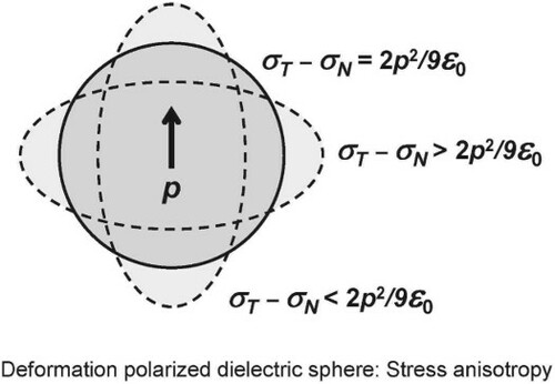The Toupin Maxwell stress tensor equation (26(26) ${\mathit{\sigma }}_d={\hat{\mathit{\sigma }}}_{\mathrm{T}}-\frac{1}{2}(\mathbf{p}\cdot \mathbf{e})\mathbf{I}+(\frac{\rho }{2}\left(\frac{\mathrm{\partial }\chi }{\mathrm{\partial }\rho }\right){\mathbf{e}}^2-P_{sr})\mathbf{I}$(26) ) is therefore anisotropic only for systems with a finite transverse polarisation component. The implication is that the dielectric stress tensor in an uniform slab polarised by a normal field is isotropic contrary to the Helmholtz–Maxwell stress tensor derived in Landau and Lifshitz [30]. The reason for this at first puzzling discrepancy is the difference in electric boundary conditions. The Helmholtz–Maxwell form is the stress induced in a slab by ‘compliant’ electrodes glued to its surface maintained at constant potential (see, e.g. [22]). The Toupin–Maxwell form is the dielectric stress in an isolated slab in a fixed external field.

3. Variational electrostatics of rigid dielectric continua

3.1. Vector potential as additional variational parameter

The displacement field in pure dielectric material is transversal (Equation 10(10) $\mathrm{div}\mathbf{d}=0$(10) ). The variational scheme developed by Ericksen exploits this special property focusing on the dielectric self displacement $\hat{\mathbf{d}}$ instead of the electric self field $\hat{\mathbf{e}}$. First, the field energy of Equation (8(8) $e_{\mathrm{E}}(\mathbf{p})=-\mathbf{p}\cdot {\mathbf{e}}_0+\frac{{ϵ}_0{\hat{\mathbf{e}}}^2}{2}$(8) ) is expressed in terms of $\hat{\mathbf{d}}$ and the polarisation $\mathbf{p}$ using Equation (14(14) $\hat{\mathbf{d}}={ϵ}_0\hat{\mathbf{e}}+\mathbf{p}$(14) ) (31) $e_{\mathrm{E}}(\mathbf{p})=-\mathbf{p}\cdot {\mathbf{e}}_0+\frac{1}{2{ϵ}_0}{(\hat{\mathbf{d}}-\mathbf{p})}^2$(31) The self displacement field is divergence free (Equation13(13) $\begin{array}{rl}\mathrm{div}\hat{\mathbf{d}}& =0\end{array}$(13) ). Ericksen imposes this constraint by representing $\hat{\mathbf{d}}$ in terms of a vector potential $\hat{\mathbf{a}}$ (32) $\hat{\mathbf{d}}=\mathbf{c}\mathbf{u}\mathbf{r}\mathbf{l}\hat{\mathbf{a}}$(32) The vector field $\hat{\mathbf{a}}$ is treated as a second independent electric variational parameter in addition to $\mathbf{p}$. The corresponding two-variable electrostatic energy density ${\tilde{e}}_{\mathrm{E}}(\mathbf{p},\hat{\mathbf{a}})$ is found by substituting Equation (32(32) $\hat{\mathbf{d}}=\mathbf{c}\mathbf{u}\mathbf{r}\mathbf{l}\hat{\mathbf{a}}$(32) ) in Equation (31(31) $e_{\mathrm{E}}(\mathbf{p})=-\mathbf{p}\cdot {\mathbf{e}}_0+\frac{1}{2{ϵ}_0}{(\hat{\mathbf{d}}-\mathbf{p})}^2$(31) ) (33) ${\tilde{e}}_{\mathrm{E}}(\mathbf{p},\hat{\mathbf{a}})=-\mathbf{p}\cdot {\mathbf{e}}_0+\frac{{(\mathbf{c}\mathbf{u}\mathbf{r}\mathbf{l}\hat{\mathbf{a}}-\mathbf{p})}^2}{2{ϵ}_0}$(33) with the corresponding extended electrostatic energy functional (34) ${\tilde{\mathcal{E}}}_{\mathrm{E}}[\mathbf{p},\hat{\mathbf{a}}]={\int }_V{\tilde{e}}_{\mathrm{E}}(\mathbf{p},\hat{\mathbf{a}})\mathrm{d}v$(34) The reason that the extremisation of Equation (34(34) ${\tilde{\mathcal{E}}}_{\mathrm{E}}[\mathbf{p},\hat{\mathbf{a}}]={\int }_V{\tilde{e}}_{\mathrm{E}}(\mathbf{p},\hat{\mathbf{a}})\mathrm{d}v$(34) ) leads to a valid solution for the electrostatics is that the Euler–Lagrange equation for $\hat{\mathbf{a}}$ is equivalent to the Maxwell equation for the self field (Equation 12(12) $\begin{array}{rl}\mathbf{c}\mathbf{u}\mathbf{r}\mathbf{l}\hat{\mathbf{e}}& =0\end{array}$(12) ) [17]. Changing $\hat{\mathbf{a}}$ to $\hat{\mathbf{a}}+\delta \hat{\mathbf{a}}$ keeping $\mathbf{p}$ fixed yields a first order change in electrostatic energy $\delta {\tilde{\mathcal{E}}}_{\mathrm{E}}=\frac{1}{{ϵ}_0}{\int }_V(\mathbf{c}\mathbf{u}\mathbf{r}\mathbf{l}\hat{\mathbf{a}}-\mathbf{p})\cdot \mathbf{c}\mathbf{u}\mathbf{r}\mathbf{l}\delta \hat{\mathbf{a}}\mathrm{d}v$where we have used that $\delta (\mathbf{c}\mathbf{u}\mathbf{r}\mathbf{l}\hat{\mathbf{a}})=\mathbf{c}\mathbf{u}\mathbf{r}\mathbf{l}\delta \hat{\mathbf{a}}$. Converting the integrand using the vector identity Equation (A1(A1) $\begin{array}{rl}\mathrm{div}(\mathbf{u}\times \mathbf{v})& =\mathbf{v}\cdot \left(\mathbf{c}\mathbf{u}\mathbf{r}\mathbf{l}\mathbf{u}\right)-\mathbf{u}\cdot \left(\mathbf{c}\mathbf{u}\mathbf{r}\mathbf{l}\mathbf{v}\right)\end{array}$(A1) ) we can then apply the divergence theorem and obtain (35) $\begin{array}{rl}\delta {\tilde{\mathcal{E}}}_{\mathrm{E}}& =\frac{1}{{ϵ}_0}{\int }_V\mathbf{c}\mathbf{u}\mathbf{r}\mathbf{l}(\mathbf{c}\mathbf{u}\mathbf{r}\mathbf{l}\hat{\mathbf{a}}-\mathbf{p})\cdot \delta \hat{\mathbf{a}}\mathrm{d}v\\ & +\frac{1}{{ϵ}_0}{\int }_{\mathrm{\partial }V}{\mathbf{n}}_{\mathrm{\partial }V}\wedge (\mathbf{c}\mathbf{u}\mathbf{r}\mathbf{l}\hat{\mathbf{a}}-\mathbf{p})\cdot \delta \hat{\mathbf{a}}\mathrm{d}s\end{array}$(35) where $\mathrm{\partial }V$ is the boundary of V with normal ${\mathbf{n}}_{\mathrm{\partial }V}$. While $\mathbf{p}$ is strictly zero beyond the periphery of a finite dielectric body the vector potential $\hat{\mathbf{a}}$, similar to $\hat{\mathbf{e}}$ is not. However, we can assume that $\hat{\mathbf{a}}$ decays to zero with increasing distance from the dielectric body and can be neglected at the vacuum boundary $\mathrm{\partial }V$ leaving only the spatial integral over V. This assumption is justified if the dielectric carries no net charge (polarisation charge ingrates to zero). Then with the usual argument in variational theory the integral can only vanish for arbitrary $\delta \hat{\mathbf{a}}$ if (36) $\mathbf{c}\mathbf{u}\mathbf{r}\mathbf{l}(\mathbf{c}\mathbf{u}\mathbf{r}\mathbf{l}\hat{\mathbf{a}}-\mathbf{p})=0$(36) validating the identification (37) $\hat{\mathbf{e}}=(\mathbf{c}\mathbf{u}\mathbf{r}\mathbf{l}\hat{\mathbf{a}}-\mathbf{p})/{ϵ}_0$(37) with $\hat{\mathbf{e}}$ satisfying Equation (12(12) $\begin{array}{rl}\mathbf{c}\mathbf{u}\mathbf{r}\mathbf{l}\hat{\mathbf{e}}& =0\end{array}$(12) ).

As pointed out by Ericksen, there seems to be more to Equation (36(36) $\mathbf{c}\mathbf{u}\mathbf{r}\mathbf{l}(\mathbf{c}\mathbf{u}\mathbf{r}\mathbf{l}\hat{\mathbf{a}}-\mathbf{p})=0$(36) ) than this. Expanding the repeated curl using Equation (A2(A2) $\begin{array}{rl}\mathbf{c}\mathbf{u}\mathbf{r}\mathbf{l}\mathbf{c}\mathbf{u}\mathbf{r}\mathbf{l}\mathbf{u}& =\mathbf{g}\mathbf{r}\mathbf{a}\mathbf{d}\mathrm{div}\mathbf{u}-\mathrm{\Delta }\mathbf{u}\end{array}$(A2) ) we can write (38) $\mathbf{g}\mathbf{r}\mathbf{a}\mathbf{d}\left(\mathrm{div}\hat{\mathbf{a}}\right)-\mathrm{\Delta }\hat{\mathbf{a}}=\mathbf{c}\mathbf{u}\mathbf{r}\mathbf{l}\mathbf{p}$(38) Equation (38(38) $\mathbf{g}\mathbf{r}\mathbf{a}\mathbf{d}\left(\mathrm{div}\hat{\mathbf{a}}\right)-\mathrm{\Delta }\hat{\mathbf{a}}=\mathbf{c}\mathbf{u}\mathbf{r}\mathbf{l}\mathbf{p}$(38) ) suggests to introduce a transverse gauge $\mathrm{div}\hat{\mathbf{a}}=0$ familiar from Maxwell theory for electromagnetic fields. The question is, however, whether this is compatible with Maxwell jump conditions at boundaries. Ericksen argues that this is indeed the case simplifying Equation (38(38) $\mathbf{g}\mathbf{r}\mathbf{a}\mathbf{d}\left(\mathrm{div}\hat{\mathbf{a}}\right)-\mathrm{\Delta }\hat{\mathbf{a}}=\mathbf{c}\mathbf{u}\mathbf{r}\mathbf{l}\mathbf{p}$(38) ) to (39) $\mathrm{\Delta }\hat{\mathbf{a}}=-\mathbf{c}\mathbf{u}\mathbf{r}\mathbf{l}\mathbf{p}$(39) The vector potential $\hat{\mathbf{a}}$ can therefore be used as a mathematically convenient representation of transverse polarisation. In special geometries where polarisation is longitudinal $\hat{\mathbf{a}}$ is a solution of the vacuum Poisson equation and can in effect be ignored.

3.2. Varying the polarisation at fixed vector potential

In order to apply the dielectric vector potential scheme to the simple dielectric liquid its free energy functional of Equation (1(1) ${\mathcal{F}}_{\mathrm{d}}[\rho ,\mathbf{p}]={\mathcal{F}}_M[\rho ]+{\mathcal{F}}_P[\rho ,\mathbf{p}]+{\mathcal{E}}_F[\mathbf{p}]$(1) ) is extended to (40) ${\tilde{\mathcal{F}}}_{\mathrm{d}}[\rho ,\mathbf{p},\hat{\mathbf{a}}]={\mathcal{F}}_{sr}[\rho ]+{\mathcal{F}}_P[\rho ,\mathbf{p}]+{\tilde{\mathcal{E}}}_{\mathrm{E}}[\mathbf{p},\hat{\mathbf{a}}]$(40) with the electrostatic energy as given in Equation (34(34) ${\tilde{\mathcal{E}}}_{\mathrm{E}}[\mathbf{p},\hat{\mathbf{a}}]={\int }_V{\tilde{e}}_{\mathrm{E}}(\mathbf{p},\hat{\mathbf{a}})\mathrm{d}v$(34) ). The short range and polarisation terms are not modified and are still equal to the integrals of Equation (3(3) ${\mathcal{F}}_{sr}[\rho ]={\int }_{\mathrm{\Omega }}\varphi (\rho )\mathrm{d}v$(3) ) respectively Equation (4(4) ${\mathcal{F}}_P[\rho ,\mathbf{p}]={\int }_{\mathrm{\Omega }}\frac{{\mathbf{p}}^2}{2\chi (\rho )}\mathrm{d}v$(4) ). The crucial difference with the variational problem defined by Equation (1(1) ${\mathcal{F}}_{\mathrm{d}}[\rho ,\mathbf{p}]={\mathcal{F}}_M[\rho ]+{\mathcal{F}}_P[\rho ,\mathbf{p}]+{\mathcal{E}}_F[\mathbf{p}]$(1) ) is that the variation in $\mathbf{p}$ is now carried out at fixed $\hat{\mathbf{a}}$. This greatly simplifies the expression for the first order change of the electrostatic energy induced by a change of polarisation $\mathbf{p}\to \mathbf{p}+\delta \mathbf{p}$ which is $\delta {\tilde{\mathcal{E}}}_{\mathrm{E}}={\int }_{\mathrm{\Omega }}(-{\mathbf{e}}_0-\frac{1}{{ϵ}_0}(\mathbf{c}\mathbf{u}\mathbf{r}\mathbf{l}\hat{\mathbf{a}}-\mathbf{p}))\cdot \delta \mathbf{p}\mathrm{d}v$Integration can again be limited to Ω because the polarisation remains confined to the body. To this we must add the first-order change in ${\mathcal{F}}_P$ which leads to the Euler Lagrange equation (41) $\frac{\mathrm{\partial }\psi }{\mathrm{\partial }\mathbf{p}}={\mathbf{e}}_0+\frac{1}{{ϵ}_0}(\mathbf{c}\mathbf{u}\mathbf{r}\mathbf{l}\hat{\mathbf{a}}-\mathbf{p})$(41) where ψ is the local energy density defined in Equation(15(15) $\psi (\rho ,\mathbf{p})=\varphi (\rho )+\frac{{\mathbf{p}}^2}{2\chi (\rho )}$(15) ). Substituting Equation (37(37) $\hat{\mathbf{e}}=(\mathbf{c}\mathbf{u}\mathbf{r}\mathbf{l}\hat{\mathbf{a}}-\mathbf{p})/{ϵ}_0$(37) ) and combining the applied and self field using Equation (9(9) $\mathbf{e}={\mathbf{e}}_0+\hat{\mathbf{e}}$(9) ) we recover the constitutive equation for polarisation Equation (17(17) $\mathbf{p}=\chi \mathbf{e}$(17) ). Variation in density would give a third Euler–Lagrange equation. Because density is not appearing as an explicit variable in the electrostatic energy ${\tilde{e}}_{\mathrm{E}}(\mathbf{p},\hat{\mathbf{a}})$ we end up with the regular DFT equation  (16(16) ${\left(\frac{\mathrm{\partial }\psi }{\mathrm{\partial }\rho }\right)}_{\mathbf{p}}=\mu -v_{ext}$(16) ).

The Euler–Lagrange equations of the Ericksen scheme are the dielectric equations we were aiming for. Legendre transformation of the dielectric energy functional equation (1(1) ${\mathcal{F}}_{\mathrm{d}}[\rho ,\mathbf{p}]={\mathcal{F}}_M[\rho ]+{\mathcal{F}}_P[\rho ,\mathbf{p}]+{\mathcal{E}}_F[\mathbf{p}]$(1) ) as required by schemes based on using the electric potential can therefore be avoided (see Section 1). Ericksen's proof that the corresponding stationary state is also a minimum relies on Equation (6(6) ${\mathcal{E}}_F={\int }_V\frac{{ϵ}_0{\mathbf{e}}_0^2}{2}\mathrm{d}v+{\mathcal{U}}_F$(6) ) with the internal energy ${\mathcal{U}}_F$ given by Equation (7(7) ${\mathcal{U}}_F={\int }_V{e}_{\mathrm{E}}(\mathbf{p})\mathrm{d}v\equiv {\mathcal{E}}_{\mathrm{E}}$(7) ) and energy density equation (8(8) $e_{\mathrm{E}}(\mathbf{p})=-\mathbf{p}\cdot {\mathbf{e}}_0+\frac{{ϵ}_0{\hat{\mathbf{e}}}^2}{2}$(8) ). The full Maxwell Lorentz energy equation (5(5) ${\mathcal{E}}_F={\int }_V\frac{{ϵ}_0{\mathbf{e}}^2}{2}\mathrm{d}v$(5) ) is manifestly convex. The energy of the vacuum field is a constant and, hence the field energy functional ${\mathcal{E}}_{\mathrm{E}}$ is convex. This desirable property is not immediately obvious from Equation (8(8) $e_{\mathrm{E}}(\mathbf{p})=-\mathbf{p}\cdot {\mathbf{e}}_0+\frac{{ϵ}_0{\hat{\mathbf{e}}}^2}{2}$(8) ) and is also questionable for the extended dielectric models (see, e.g. Ref. [36]) favoured in the computationally oriented literature in physical chemistry [3,6–9]. Let us therefore reiterate the conditions for the validity mentioned in Section 2.1. These equations apply for a finite dielectric body in a container. The container must be large enough for the self dielectric displacement field $\hat{\mathbf{d}}$ to decay sufficiently fast outside the dielectric so that it can be neglected at the boundaries $\mathrm{\partial }V$ of the container. We already made use of this property when discarding the surface term in Equation (35(35) $\begin{array}{rl}\delta {\tilde{\mathcal{E}}}_{\mathrm{E}}& =\frac{1}{{ϵ}_0}{\int }_V\mathbf{c}\mathbf{u}\mathbf{r}\mathbf{l}(\mathbf{c}\mathbf{u}\mathbf{r}\mathbf{l}\hat{\mathbf{a}}-\mathbf{p})\cdot \delta \hat{\mathbf{a}}\mathrm{d}v\\ & +\frac{1}{{ϵ}_0}{\int }_{\mathrm{\partial }V}{\mathbf{n}}_{\mathrm{\partial }V}\wedge (\mathbf{c}\mathbf{u}\mathbf{r}\mathbf{l}\hat{\mathbf{a}}-\mathbf{p})\cdot \delta \hat{\mathbf{a}}\mathrm{d}s\end{array}$(35) ). For the detailed proof, we refer to Ericksen's paper [17] (see also the discussion in Ref. [23]).

4. Transformation to an arbitrary reference frame

4.1. Maxwell equations in Lagrangian representation

In the Lagrangian or material formulation of continuum mechanics, the state of a system is described in terms of a deformation from a reference state also called material state. The deformed state is called the current or spatial state. This is how constitutive stress–strain relations are specified in the theory of non-linear elasticity [25]. In fluid mechanics, this is not necessary. This, however, does not prohibit a Lagrangian description of equilibrium fluids and, in fact, offers a way of deriving expressions for stress tensors using the established mathematical machinery of the theory of nonlinear elasticity (for an instructive example, see  [37]). Obviously, the reference frame is now arbitrary and any result, once transformed back to current space, should have lost all traces of the reference frame.

First we list the necessary kinematics. The central mathematical construct is a vector function $\mathit{\chi }(\mathbf{X})$ mapping points $\mathbf{X}$ in the reference space $B_r$ to points $\mathbf{x}$ in the current space B so that $\mathbf{x}=\mathit{\chi }(\mathbf{X})$. Strain in elastic solids is not directly equal to displacement $\mathit{\chi }(\mathbf{X})$ but is computed from the deformation gradient tensor (42) $F_{i\alpha }=\frac{\mathrm{\partial }{x}_i}{\mathrm{\partial }{X}_{\alpha }}$(42) where Cartesian coordinates in current and reference space are written as $(x_i,i=1,2,3)$ and $(X_{\alpha },\alpha =1,2,3)$, respectively. In continuum mechanical theory, direct vector notation is often more convenient. To change the notation of a derivative operator in current space ($\mathbf{g}\mathbf{r}\mathbf{a}\mathbf{d},\mathrm{div},\mathbf{c}\mathbf{u}\mathbf{r}\mathbf{l}$) to the corresponding derivative operator in reference space the first letter of the operator name is switched to upper case. In this convention, the deformation gradient tensor of Equation (42(42) $F_{i\alpha }=\frac{\mathrm{\partial }{x}_i}{\mathrm{\partial }{X}_{\alpha }}$(42) ) is written as (43) $\mathbf{F}=\mathbf{G}\mathbf{r}\mathbf{a}\mathbf{d}\mathit{\chi }={\left({\mathrm{\nabla }}_X\mathbf{x}\right)}^{\mathrm{T}}$(43) where ${\mathrm{\nabla }}_X$ is the nabla operator in the reference configuration and ${}^{\mathrm{T}}$ denotes the transpose. (Note the difference between the $\mathbf{G}\mathbf{r}\mathbf{a}\mathbf{d}$ and ${\mathrm{\nabla }}_X$ operators when acting on vectors. The order of the ($i,\alpha$) indices is exchanged [37].) Gradients of $\mathbf{F}$ are converted according to (44) ${\mathrm{\nabla }}_X={\mathbf{F}}^{\mathrm{T}}\mathrm{\nabla },\mathrm{\nabla }={\mathbf{F}}^{-\mathrm{T}}{\mathrm{\nabla }}_X$(44) with ${\mathbf{F}}^{-\mathrm{T}}=({\mathbf{F}}^{-1}{)}^T$. Number density (in non-reactive systems) is conserved and hence the spatial density ρ is related to the density ${\rho }_0$ in reference space as (45) $J\rho ={\rho }_0$(45) where J is the Jacobian of the deformation gradient tensor (46) $J=det\mathbf{F}$(46) J is positive.

The electric field $\mathbf{e}$ and displacement field $\mathbf{d}$ in Maxwell theory are tied to their source charge densities by differential equations. Position derivatives change switching over from the current to the reference frame (Equation 44(44) ${\mathrm{\nabla }}_X={\mathbf{F}}^{\mathrm{T}}\mathrm{\nabla },\mathrm{\nabla }={\mathbf{F}}^{-\mathrm{T}}{\mathrm{\nabla }}_X$(44) ) suggesting that $\mathbf{e}$ and $\mathbf{d}$ cannot simply remain the same when expressed in the reference frame. The central idea in Lagrangian electromechanics is to adjust $\mathbf{e}$ and $\mathbf{d}$ making the Maxwell equations form invariant [26]. The Lagrangian counterparts of the electric field $\mathbf{e}$ and displacement $\mathbf{d}$ are denoted by capital $\mathbf{E}$ and $\mathbf{D}$ respectively and are obtained from the fields in current space according to (47) $\begin{array}{rl}\mathbf{E}& ={\mathbf{F}}^{\mathrm{T}}\mathbf{e}\end{array}$(47) (48) $\begin{array}{rl}\mathbf{D}& =J{\mathbf{F}}^{-1}\mathbf{d}\end{array}$(48) With these transformation rules, the dielectric Maxwell equations are written in the reference frame as (49) $\mathbf{C}\mathbf{u}\mathbf{r}\mathbf{l}\mathbf{E}=0,\mathrm{Div}\mathbf{D}=0$(49) where $\mathbf{C}\mathbf{u}\mathbf{r}\mathbf{l}$ and $\mathrm{Div}$ are the curl and divergence operators applied in reference coordinates $\mathbf{X}$. The equations for the material electric and displacement field have the same form as in the current frame. Note also that $\mathbf{D}\cdot \mathbf{E}=J\mathbf{d}\cdot \mathbf{e}$. The inproduct of $\mathbf{d}$ and $\mathbf{e}$ is transformed as a density. However, non-equilibrium electrostatic energy is determined, not by $\mathbf{d}\cdot \mathbf{e}$, but by $\mathbf{e}\cdot \mathbf{e}$, which is not behaving as a density under transformation. This is how in Lagrangian theory the geometry dependence of the energy is captured.

While the transformation rules for electric field and dielectric displacement are imposed by requiring the preservation (form invariance) of the Maxwell equations the Lagrangian form $\mathbf{P}$ of polarisation is open to some choice. We follow Dorfmann and Ogden [23,26] and define $\mathbf{P}$ as (50) $\mathbf{P}=J{\mathbf{F}}^{-1}\mathbf{p}$(50) which is the same rule as for the displacement field (Equation 48(48) $\begin{array}{rl}\mathbf{D}& =J{\mathbf{F}}^{-1}\mathbf{d}\end{array}$(48) ). Combining Equations (47(47) $\begin{array}{rl}\mathbf{E}& ={\mathbf{F}}^{\mathrm{T}}\mathbf{e}\end{array}$(47) ), (48(48) $\begin{array}{rl}\mathbf{D}& =J{\mathbf{F}}^{-1}\mathbf{d}\end{array}$(48) ) and (50(50) $\mathbf{P}=J{\mathbf{F}}^{-1}\mathbf{p}$(50) ) gives (51) $\mathbf{D}={ϵ}_{0}J{\mathbf{C}}^{-1}\mathbf{E}+\mathbf{P}$(51) with $\mathbf{C}$ the right Cauchy–Green strain tensor. (52) $\mathbf{C}={\mathbf{F}}^{\mathrm{T}}\mathbf{F},$(52) We must accept that the fundamental Maxwell–Lorentz relation $\mathbf{d}={ϵ}_0\mathbf{e}+\mathbf{p}$ cannot be carried over from the current frame to the reference frame. This is inevitable because $\mathbf{e}$ and $\mathbf{d}$ transform according to different rules (Equations 47(47) $\begin{array}{rl}\mathbf{E}& ={\mathbf{F}}^{\mathrm{T}}\mathbf{e}\end{array}$(47) and 48(48) $\begin{array}{rl}\mathbf{D}& =J{\mathbf{F}}^{-1}\mathbf{d}\end{array}$(48) ). In this respect, the relation $\mathbf{d}={ϵ}_0\mathbf{e}+\mathbf{p}$, although universal, is similar to a constitutive equation [28].

4.2. Material specification of the simple dielectric fluid

The electric fields used in the variational treatment of the simple dielectric fluid in Section 3 were not $\mathbf{e}$ and $\mathbf{d}$ but the self fields $\hat{\mathbf{e}}$ and $\hat{\mathbf{d}}$. Of course the same transformation rules apply to the Lagrangian versions of self fields. Indicating the Lagrangian self fields again in capitals keeping the hat we have (53) $\begin{array}{rl}\hat{\mathbf{E}}& ={\mathbf{F}}^{\mathrm{T}}\hat{\mathbf{e}}\end{array}$(53) (54) $\begin{array}{rl}\hat{\mathbf{D}}& =J{\mathbf{F}}^{-1}\hat{\mathbf{d}}\end{array}$(54) satisfying Maxwell equations in agreement with Equation(49(49) $\mathbf{C}\mathbf{u}\mathbf{r}\mathbf{l}\mathbf{E}=0,\mathrm{Div}\mathbf{D}=0$(49) ) (55) $\mathbf{C}\mathbf{u}\mathbf{r}\mathbf{l}\hat{\mathbf{E}}=0,\mathrm{Div}\hat{\mathbf{D}}=0$(55) with the self field Lagrangian Lorentz equation  (51(51) $\mathbf{D}={ϵ}_{0}J{\mathbf{C}}^{-1}\mathbf{E}+\mathbf{P}$(51) ) (56) ${ϵ}_0\hat{\mathbf{E}}=J^{-1}\mathbf{C}(\hat{\mathbf{D}}-\mathbf{P})$(56) arranged in the form it will be applied in the following.

The task we have now is to express the free energy functional as used in Section 3 in material form. We do this term by term starting with the electrostatic field energy of $e_{\mathrm{E}}(\mathbf{p})$ of Equation (31(31) $e_{\mathrm{E}}(\mathbf{p})=-\mathbf{p}\cdot {\mathbf{e}}_0+\frac{1}{2{ϵ}_0}{(\hat{\mathbf{d}}-\mathbf{p})}^2$(31) ). There are two contributions, a term coupling polarisation to the external field and the electrostatic self energy. It will be convenient to treat these terms separately. The interaction with the external field will be from now on indicated by ${\mathcal{E}}_I$ (57) ${\mathcal{E}}_I=-{\int }_V\mathbf{p}\cdot {\mathbf{e}}_0\mathrm{d}v$(57) Applying the inverse of Equations (47(47) $\begin{array}{rl}\mathbf{E}& ={\mathbf{F}}^{\mathrm{T}}\mathbf{e}\end{array}$(47) ) and (50(50) $\mathbf{P}=J{\mathbf{F}}^{-1}\mathbf{p}$(50) ) gives the material representation of ${\mathcal{E}}_I$ which is a functional of the polarisation $\mathbf{P}$ in the reference frame and deformation gradient $\mathbf{F}$ (58) $\begin{array}{rl}{\tilde{\mathcal{E}}}_I(\mathbf{P},\mathbf{F})& =-{\int }_V{J}^{-1}\left(\mathbf{F}\mathbf{P}\right)\cdot \left({\mathbf{F}}^{-\mathrm{T}}{\mathbf{E}}_0\right)J\mathrm{d}V\\ & =-{\int }_V\mathbf{P}\cdot {\mathbf{E}}_0\mathrm{d}V\end{array}$(58) $\mathrm{d}V=J^{-1}\mathrm{d}v$ is a reference space volume element. The factors J cancel. Similar to $\mathbf{d}\cdot \mathbf{e}$ the inproduct $\mathbf{p}\cdot \mathbf{e}$ also transforms as a density. Note, however, that ${\mathbf{E}}_0={\mathbf{F}}^{\mathrm{T}}{\mathbf{e}}_0$ varies with deformation because ${\mathbf{e}}_0$ is fixed implying that also the external field interaction Equation (58(58) $\begin{array}{rl}{\tilde{\mathcal{E}}}_I(\mathbf{P},\mathbf{F})& =-{\int }_V{J}^{-1}\left(\mathbf{F}\mathbf{P}\right)\cdot \left({\mathbf{F}}^{-\mathrm{T}}{\mathbf{E}}_0\right)J\mathrm{d}V\\ & =-{\int }_V\mathbf{P}\cdot {\mathbf{E}}_0\mathrm{d}V\end{array}$(58) ) is sensitive to changes in shape and will therefore contribute to the stress.

Next we rewrite the self interaction energy for which we also introduce a separate symbol (59) ${\mathcal{E}}_S={\int }_V\frac{1}{2{ϵ}_0}{(\hat{\mathbf{d}}-\mathbf{p})}^2\mathrm{d}v$(59) Applying Equations (47(47) $\begin{array}{rl}\mathbf{E}& ={\mathbf{F}}^{\mathrm{T}}\mathbf{e}\end{array}$(47) ), (48(48) $\begin{array}{rl}\mathbf{D}& =J{\mathbf{F}}^{-1}\mathbf{d}\end{array}$(48) ) and (50(50) $\mathbf{P}=J{\mathbf{F}}^{-1}\mathbf{p}$(50) ) we can write ${\mathcal{E}}_S$ as (60) $\begin{array}{rl}{\mathcal{E}}_S& ={\int }_v\frac{1}{2{ϵ}_0}\left(J^{-1}\mathbf{F}(\hat{\mathbf{D}}-\mathbf{P})\right)\cdot \left(J^{-1}\mathbf{F}(\hat{\mathbf{D}}-\mathbf{P})\right)J\mathrm{d}V\\ & ={\int }_V\frac{J^{-1}}{2{ϵ}_0}(\hat{\mathbf{D}}-\mathbf{P})\cdot \mathbf{C}(\hat{\mathbf{D}}-\mathbf{P})\mathrm{d}V\end{array}$(60) where in the second step we have substituted Equation(52(52) $\mathbf{C}={\mathbf{F}}^{\mathrm{T}}\mathbf{F},$(52) ). In preparation for a repeat of the derivation of Section 3, we represent $\hat{\mathbf{D}}$ in terms of a vector potential $\hat{\mathbf{A}}$. The field transformation rules Equations (47(47) $\begin{array}{rl}\mathbf{E}& ={\mathbf{F}}^{\mathrm{T}}\mathbf{e}\end{array}$(47) ) and (48(48) $\begin{array}{rl}\mathbf{D}& =J{\mathbf{F}}^{-1}\mathbf{d}\end{array}$(48) ) ensure that a solution to the Maxwell equations equation (55(55) $\mathbf{C}\mathbf{u}\mathbf{r}\mathbf{l}\hat{\mathbf{E}}=0,\mathrm{Div}\hat{\mathbf{D}}=0$(55) ) also satisfies the original Maxwell equations in the current frame. Therefore, in direct correspondence to Equation (32(32) $\hat{\mathbf{d}}=\mathbf{c}\mathbf{u}\mathbf{r}\mathbf{l}\hat{\mathbf{a}}$(32) ), we set (61) $\hat{\mathbf{D}}=\mathbf{C}\mathbf{u}\mathbf{r}\mathbf{l}\hat{\mathbf{A}}$(61) and extend the self energy functional to a three variable energy functional (62) $\begin{array}{rl}{\tilde{\mathcal{E}}}_S[\mathbf{P},\hat{\mathbf{A}},\mathbf{F}]& ={\int }_V\frac{J^{-1}}{2{ϵ}_0}(\mathbf{C}\mathbf{u}\mathbf{r}\mathbf{l}\hat{\mathbf{A}}-\mathbf{P})\\ & \cdot \mathbf{C}(\mathbf{C}\mathbf{u}\mathbf{r}\mathbf{l}\hat{\mathbf{A}}-\mathbf{P})\mathrm{d}V\end{array}$(62) The sum (63) ${\tilde{\mathcal{E}}}_{\mathrm{E}}[\mathbf{P},\hat{\mathbf{A}},\mathbf{F}]={\tilde{\mathcal{E}}}_I[\mathbf{P},\mathbf{F}]+{\tilde{\mathcal{E}}}_S[\mathbf{P},\hat{\mathbf{A}},\mathbf{F}]$(63) is the continuum mechanics adaptation of Equation (34(34) ${\tilde{\mathcal{E}}}_{\mathrm{E}}[\mathbf{p},\hat{\mathbf{a}}]={\int }_V{\tilde{e}}_{\mathrm{E}}(\mathbf{p},\hat{\mathbf{a}})\mathrm{d}v$(34) ).

Transformation of the polarisation energy ${\mathcal{F}}_P$ (Equation 4(4) ${\mathcal{F}}_P[\rho ,\mathbf{p}]={\int }_{\mathrm{\Omega }}\frac{{\mathbf{p}}^2}{2\chi (\rho )}\mathrm{d}v$(4) ) proceeds along the same lines. Consistent with ${\tilde{\mathcal{E}}}_S$ of Equation (62(62) $\begin{array}{rl}{\tilde{\mathcal{E}}}_S[\mathbf{P},\hat{\mathbf{A}},\mathbf{F}]& ={\int }_V\frac{J^{-1}}{2{ϵ}_0}(\mathbf{C}\mathbf{u}\mathbf{r}\mathbf{l}\hat{\mathbf{A}}-\mathbf{P})\\ & \cdot \mathbf{C}(\mathbf{C}\mathbf{u}\mathbf{r}\mathbf{l}\hat{\mathbf{A}}-\mathbf{P})\mathrm{d}V\end{array}$(62) ) the dependence on polarisation is specified in terms of the material representation $\mathbf{P}$ (Equation 50(50) $\mathbf{P}=J{\mathbf{F}}^{-1}\mathbf{p}$(50) ) which plays role of independent variational degree of freedom. This introduces again the strain tensor $\mathbf{C}$ as an effective coupling matrix. A further effect of deformation is through the susceptibility which varies with density. Using Equation (45(45) $J\rho ={\rho }_0$(45) ) we write $\chi (\rho )=\chi (J^{-1}{\rho }_0)$. The result is a material polarisation energy functional (64) ${\tilde{\mathcal{F}}}_P[\mathbf{P},\mathbf{F}]={\int }_V\frac{J^{-1}}{2\chi (J^{-1}{\rho }_0)}\mathbf{P}\cdot \mathbf{C}\mathbf{P}\mathrm{d}V$(64) The transformation of the local mechanical energy Equation (3(3) ${\mathcal{F}}_{sr}[\rho ]={\int }_{\mathrm{\Omega }}\varphi (\rho )\mathrm{d}v$(3) ) is standard. (65) ${\tilde{\mathcal{F}}}_{sr}[\mathbf{F}]={\int }_{{\mathrm{\Omega }}_r}\varphi (J^{-1}{\rho }_0)J\mathrm{d}V$(65)

5. Varying the electric degrees of freedom

We will now retrace the variational procedure of Section 3 for the material electrical degrees of freedom at rigid geometry. Thus changing $\hat{\mathbf{A}}$ to $\hat{\mathbf{A}}+\delta \hat{\mathbf{A}}$ keeping $\mathbf{P}$ and $\mathbf{F}$ fixed we determine the first order change in the electrostatic field energy Equation (63(63) ${\tilde{\mathcal{E}}}_{\mathrm{E}}[\mathbf{P},\hat{\mathbf{A}},\mathbf{F}]={\tilde{\mathcal{E}}}_I[\mathbf{P},\mathbf{F}]+{\tilde{\mathcal{E}}}_S[\mathbf{P},\hat{\mathbf{A}},\mathbf{F}]$(63) ) $\delta {\tilde{\mathcal{E}}}_{\mathrm{E}}=\delta {\tilde{\mathcal{E}}}_S={\int }_V\frac{J^{-1}}{{ϵ}_0}\mathbf{C}(\mathbf{C}\mathbf{u}\mathbf{r}\mathbf{l}\hat{\mathbf{A}}-\mathbf{P})\cdot \mathbf{C}\mathbf{u}\mathbf{r}\mathbf{l}\delta \hat{\mathbf{A}}\mathrm{d}V$where have used that the Cauchy–Green strain tensor (Equation 52(52) $\mathbf{C}={\mathbf{F}}^{\mathrm{T}}\mathbf{F},$(52) ) is symmetric. Next applying the divergence theorem in reference space $\begin{array}{rl}\delta {\tilde{\mathcal{E}}}_{\mathrm{E}}& ={\int }_V\mathbf{C}\mathbf{u}\mathbf{r}\mathbf{l}\left(\frac{J^{-1}}{{ϵ}_0}\mathbf{C}(\mathbf{C}\mathbf{u}\mathbf{r}\mathbf{l}\hat{\mathbf{A}}-\mathbf{P})\right)\cdot \delta \hat{\mathbf{A}}\mathrm{d}V\\ & +{\int }_{\mathrm{\partial }V}{\mathbf{N}}_{\mathrm{\partial }V}\times \left(\frac{J^{-1}}{{ϵ}_0}\mathbf{C}(\mathbf{C}\mathbf{u}\mathbf{r}\mathbf{l}\hat{\mathbf{A}}-\mathbf{P})\right)\cdot \delta \hat{\mathbf{A}}\mathrm{d}S\end{array}$As in Section 3, we assume that the self fields vanish at the container boundary $\mathrm{\partial }V$ and we are left with the Euler–Lagrange equation (66) $\mathbf{C}\mathbf{u}\mathbf{r}\mathbf{l}\left(\frac{J^{-1}}{{ϵ}_0}\mathbf{C}(\mathbf{C}\mathbf{u}\mathbf{r}\mathbf{l}\hat{\mathbf{A}}-\mathbf{P})\right)=0$(66) Substituting Equation (61(61) $\hat{\mathbf{D}}=\mathbf{C}\mathbf{u}\mathbf{r}\mathbf{l}\hat{\mathbf{A}}$(61) ) and referring back to the modified Lorentz relation  (56(56) ${ϵ}_0\hat{\mathbf{E}}=J^{-1}\mathbf{C}(\hat{\mathbf{D}}-\mathbf{P})$(56) ) verifies that the Euler Lagrange equation for variation in $\hat{\mathbf{A}}$ recovers the Maxwell equation $\mathbf{C}\mathbf{u}\mathbf{r}\mathbf{l}\hat{\mathbf{E}}=0$ for the self field in the reference frame.

Changing $\mathbf{P}$ to $\mathbf{P}+\delta \mathbf{P}$ keeping $\hat{\mathbf{A}}$ and $\mathbf{F}$ fixed both the interaction energy equation (58(58) $\begin{array}{rl}{\tilde{\mathcal{E}}}_I(\mathbf{P},\mathbf{F})& =-{\int }_V{J}^{-1}\left(\mathbf{F}\mathbf{P}\right)\cdot \left({\mathbf{F}}^{-\mathrm{T}}{\mathbf{E}}_0\right)J\mathrm{d}V\\ & =-{\int }_V\mathbf{P}\cdot {\mathbf{E}}_0\mathrm{d}V\end{array}$(58) ) and self energy equation (60(60) $\begin{array}{rl}{\mathcal{E}}_S& ={\int }_v\frac{1}{2{ϵ}_0}\left(J^{-1}\mathbf{F}(\hat{\mathbf{D}}-\mathbf{P})\right)\cdot \left(J^{-1}\mathbf{F}(\hat{\mathbf{D}}-\mathbf{P})\right)J\mathrm{d}V\\ & ={\int }_V\frac{J^{-1}}{2{ϵ}_0}(\hat{\mathbf{D}}-\mathbf{P})\cdot \mathbf{C}(\hat{\mathbf{D}}-\mathbf{P})\mathrm{d}V\end{array}$(60) ) contribute to the first-order variation of the field energy equation (63(63) ${\tilde{\mathcal{E}}}_{\mathrm{E}}[\mathbf{P},\hat{\mathbf{A}},\mathbf{F}]={\tilde{\mathcal{E}}}_I[\mathbf{P},\mathbf{F}]+{\tilde{\mathcal{E}}}_S[\mathbf{P},\hat{\mathbf{A}},\mathbf{F}]$(63) ) $\begin{array}{rl}\delta {\tilde{\mathcal{E}}}_{\mathrm{E}}& =-{\int }_V({\mathbf{E}}_0+\frac{J^{-1}}{{ϵ}_0}\mathbf{C}(\mathbf{C}\mathbf{u}\mathbf{r}\mathbf{l}\hat{\mathbf{A}}-\mathbf{P}))\cdot \delta \mathbf{P}\mathrm{d}V\\ & =-{\int }_V({\mathbf{E}}_0+\hat{\mathbf{E}})\cdot \delta \mathbf{P}\mathrm{d}V\end{array}$where in the second step we have restored the explicit dependence on the material electric self field using Equations (61(61) $\hat{\mathbf{D}}=\mathbf{C}\mathbf{u}\mathbf{r}\mathbf{l}\hat{\mathbf{A}}$(61) ) and (56(56) ${ϵ}_0\hat{\mathbf{E}}=J^{-1}\mathbf{C}(\hat{\mathbf{D}}-\mathbf{P})$(56) ). Adding the variation in the stored polarisation energy (Equation 64(64) ${\tilde{\mathcal{F}}}_P[\mathbf{P},\mathbf{F}]={\int }_V\frac{J^{-1}}{2\chi (J^{-1}{\rho }_0)}\mathbf{P}\cdot \mathbf{C}\mathbf{P}\mathrm{d}V$(64) ) $\delta {\tilde{\mathcal{F}}}_P={\int }_V\left(\frac{J^{-1}}{\chi }\mathbf{C}\mathbf{P}\right)\cdot \delta \mathbf{P}\mathrm{d}V$leads to the Euler–Lagrange equation $\frac{J^{-1}}{\chi }\mathbf{C}\mathbf{P}={\mathbf{E}}_0+\hat{\mathbf{E}}$Resolving the Cauchy–Green tensor $\mathbf{C}$ using Equation(52(52) $\mathbf{C}={\mathbf{F}}^{\mathrm{T}}\mathbf{F},$(52) ) gives (67) $J^{-1}\mathbf{F}\mathbf{P}=\chi {\mathbf{F}}^{-\mathrm{T}}\mathbf{E}$(67) The left-hand side matches the inverse of the transformation equation (50(50) $\mathbf{P}=J{\mathbf{F}}^{-1}\mathbf{p}$(50) ) for polarisation and the right-hand side the inverse of the transformation equation (47(47) $\begin{array}{rl}\mathbf{E}& ={\mathbf{F}}^{\mathrm{T}}\mathbf{e}\end{array}$(47) ) for electric fields. Applying these transformations, we see that Equation (67(67) $J^{-1}\mathbf{F}\mathbf{P}=\chi {\mathbf{F}}^{-\mathrm{T}}\mathbf{E}$(67) ) reduces to the sought after constitutive relation  (17(17) $\mathbf{p}=\chi \mathbf{e}$(17) ) in the current frame. Note also that the material constitutive relation between $\mathbf{P}$ and $\mathbf{E}$ is still linear, but with a susceptibility coefficient varying with deformation. For finite deformation the geometry dependence is even non-linear and similar to Equation (56(56) ${ϵ}_0\hat{\mathbf{E}}=J^{-1}\mathbf{C}(\hat{\mathbf{D}}-\mathbf{P})$(56) ).

6. Variational continuum mechanics of simple liquids

6.1. Variation of deformation

So far so good. We have reproduced in a roundabout way what we had already established in Section 3 in an Eulerian framework. The ‘pull back’ to a Lagrangian frame is a device for variation of the geometry which will give the expression for the stress tensor. In nonlinear continuum mechanics, deformation is quantified as a change $\mathit{\chi }\to \mathit{\chi }+\delta \mathit{\chi }$ of the placement in current space [25]. Indicating the change $\delta \mathbf{x}$ of position by $\mathbf{u}$ we therefore have to evaluate the first-order differences induced by making the substitution (68) $\mathbf{x}(\mathbf{X})\to \mathbf{x}(\mathbf{X})+\mathbf{u}(\mathbf{X})$(68) The Lagrangian form of the energies in Section 4.2 was all functions of the deformation gradient tensor $\mathbf{F}$ defined in Equation (43(43) $\mathbf{F}=\mathbf{G}\mathbf{r}\mathbf{a}\mathbf{d}\mathit{\chi }={\left({\mathrm{\nabla }}_X\mathbf{x}\right)}^{\mathrm{T}}$(43) ) and its inverse. The first-order differential is the gradient of the change $\mathbf{u}$ in displacement evaluated in the reference frame (69) $\delta \mathbf{F}=\mathbf{G}\mathbf{r}\mathbf{a}\mathbf{d}\mathbf{u}={\left({\mathrm{\nabla }}_X\mathbf{u}\right)}^{\mathrm{T}},\delta {\mathbf{F}}^{-T}=-{\mathbf{F}}^{-\mathrm{T}}\cdot \delta {\mathbf{F}}^{\mathrm{T}}\cdot {\mathbf{F}}^{-\mathrm{T}}$(69) Another important geometric differential is the variation $\delta J$ of the determinant of $\mathbf{F}$ (Equation 46(46) $J=det\mathbf{F}$(46) ). To find $\delta J$ we apply the chain rule after first recalling Jacobi's formula (70) $\frac{\mathrm{\partial }det\mathbf{F}}{\mathrm{\partial }\mathbf{F}}=(det\mathbf{F}){\mathbf{F}}^{-1}$(70) This gives (71) $\delta J=J\mathrm{Tr}\left({\mathbf{F}}^{-1}\delta \mathbf{F}\right)=J{\mathbf{F}}^{-\mathrm{T}}:\delta \mathbf{F}$(71) where $\mathbf{A}:\mathbf{B}={\mathrm{\Sigma }}_{ij}{A}_{ij}{B}_{ij}$ stands for a double contraction of matrices $\mathbf{A}$ and $\mathbf{B}$. With Equation (45(45) $J\rho ={\rho }_0$(45) ), we have therefore for the variation in density (72) $\delta \rho =\delta \left(J^{-1}{\rho }_0\right)=-\frac{{\rho }_0}{J^2}\delta J=-\rho {\mathbf{F}}^{-\mathrm{T}}:\delta \mathbf{F}$(72) Returning to the Eulerian representation we can write (73) $\delta J=J\mathrm{div}\mathbf{u},\delta \rho =-\rho \mathrm{div}\mathbf{u}$(73) which is rather more recognisable [37]. We will also need the first order change in the Cauchy–Green matrix equation (52(52) $\mathbf{C}={\mathbf{F}}^{\mathrm{T}}\mathbf{F},$(52) ). (74) $\delta \mathbf{C}=\delta \left({\mathbf{F}}^{\mathrm{T}}\mathbf{F}\right)=\left(\delta {\mathbf{F}}^{\mathrm{T}}\right)\mathbf{F}+{\mathbf{F}}^{\mathrm{T}}\delta \mathbf{F}$(74) Equations (68(68) $\mathbf{x}(\mathbf{X})\to \mathbf{x}(\mathbf{X})+\mathbf{u}(\mathbf{X})$(68) )–(74(74) $\delta \mathbf{C}=\delta \left({\mathbf{F}}^{\mathrm{T}}\mathbf{F}\right)=\left(\delta {\mathbf{F}}^{\mathrm{T}}\right)\mathbf{F}+{\mathbf{F}}^{\mathrm{T}}\delta \mathbf{F}$(74) ) and further extensions are the subject of the first section of almost every paper in non-linear continuum mechanics under the heading of kinematics. This includes the publications cited here [17,19,22–24,26,38]. A paper we found particularly instructive in this respect, although not on electromechanics but gradient capillary stress, is  [37]. For the continuum mechanics of simple liquids the equations in this section are all what is needed.

6.2. True and nominal stress

Stress tensors in finite deformation continuum mechanics are obtained as derivatives of energy densities in reference space. Differentiation is carried out with respect to material variables and the result is then transformed back to the current frame to give the physical (Cauchy) stress [25]. Implemented in a variational framework, this requires determining the differential of the free energy functional equation (1(1) ${\mathcal{F}}_{\mathrm{d}}[\rho ,\mathbf{p}]={\mathcal{F}}_M[\rho ]+{\mathcal{F}}_P[\rho ,\mathbf{p}]+{\mathcal{E}}_F[\mathbf{p}]$(1) ) in response to deformation. As an illustration and for further reference we will go (in minimal detail) through the application to the mechanical free energy ${\mathcal{F}}_M$ of Equation (2(2) ${\mathcal{F}}_M[\rho ]={\mathcal{F}}_{sr}[\rho ]+{\int }_{\mathrm{\Omega }}{v}_{ext}(\mathbf{r})\rho (\mathbf{r})\mathrm{d}v$(2) ). The material form of the integral over local energy density $\varphi (\rho )$ was given in Equation (65(65) ${\tilde{\mathcal{F}}}_{sr}[\mathbf{F}]={\int }_{{\mathrm{\Omega }}_r}\varphi (J^{-1}{\rho }_0)J\mathrm{d}V$(65) ). The derivation of the corresponding stress and work balance is general and valid for all local density functions ϕ. In recognition of this we replace ‘sr’ suffix by ϕ.

Expanding the integral equation (65(65) ${\tilde{\mathcal{F}}}_{sr}[\mathbf{F}]={\int }_{{\mathrm{\Omega }}_r}\varphi (J^{-1}{\rho }_0)J\mathrm{d}V$(65) ), now called $\delta {\mathcal{F}}_{\varphi }$, in differentials of ϕ and J we get (75) $\delta {\mathcal{F}}_{\varphi }={\int }_{{\mathrm{\Omega }}_r}(\frac{\mathrm{\partial }\varphi }{\mathrm{\partial }\rho }J\delta \rho +\varphi \delta J)\mathrm{d}V$(75) Substituting Equations (71(71) $\delta J=J\mathrm{Tr}\left({\mathbf{F}}^{-1}\delta \mathbf{F}\right)=J{\mathbf{F}}^{-\mathrm{T}}:\delta \mathbf{F}$(71) ) and (72(72) $\delta \rho =\delta \left(J^{-1}{\rho }_0\right)=-\frac{{\rho }_0}{J^2}\delta J=-\rho {\mathbf{F}}^{-\mathrm{T}}:\delta \mathbf{F}$(72) ) gives (76) $\delta {\mathcal{F}}_{\varphi }={\int }_{{\mathrm{\Omega }}_r}J(-\rho \frac{\mathrm{\partial }\varphi }{\mathrm{\partial }\rho }+\varphi ){\mathbf{F}}^{-\mathrm{T}}:\delta \mathbf{F}\mathrm{d}V$(76) Equation (76(76) $\delta {\mathcal{F}}_{\varphi }={\int }_{{\mathrm{\Omega }}_r}J(-\rho \frac{\mathrm{\partial }\varphi }{\mathrm{\partial }\rho }+\varphi ){\mathbf{F}}^{-\mathrm{T}}:\delta \mathbf{F}\mathrm{d}V$(76) ) has the form of incremental internal work expressed in material quantities (77) $W_{\mathrm{int}}={\int }_{{\mathrm{\Omega }}_r}\mathbf{\Sigma }:\delta \mathbf{F}\mathrm{d}V$(77) Equation (77(77) $W_{\mathrm{int}}={\int }_{{\mathrm{\Omega }}_r}\mathbf{\Sigma }:\delta \mathbf{F}\mathrm{d}V$(77) ) is fundamental in non-linear continuum mechanics defining the Lagrangian stress tensor $\mathbf{\Sigma }$. This quantity is also referred to as the nominal [25] or first Piola–Kirchhoff stress tensor. We abbreviate this to simply the Piola stress tensor in the following. The Piola stress tensor for the local mechanics specified by ϕ is therefore (78) ${\mathbf{\Sigma }}_{\varphi }=J(-\rho \frac{\mathrm{\partial }\varphi }{\mathrm{\partial }\rho }+\varphi ){\mathbf{F}}^{-\mathrm{T}}$(78) The Piola stress tensor $\mathbf{\Sigma }$ and the true (Cauchy) stress tensor $\mathit{\sigma }$ in current space are related by a ‘pull back’ and the inverse ‘push forward’ transformation [25] (79) $\mathbf{\Sigma }=J\mathit{\sigma }{\mathbf{F}}^{-\mathrm{T}},\mathit{\sigma }=J^{-1}\mathbf{\Sigma }{\mathbf{F}}^{\mathrm{T}}$(79) Inserting in Equation (77(77) $W_{\mathrm{int}}={\int }_{{\mathrm{\Omega }}_r}\mathbf{\Sigma }:\delta \mathbf{F}\mathrm{d}V$(77) ) and using Equation (69(69) $\delta \mathbf{F}=\mathbf{G}\mathbf{r}\mathbf{a}\mathbf{d}\mathbf{u}={\left({\mathrm{\nabla }}_X\mathbf{u}\right)}^{\mathrm{T}},\delta {\mathbf{F}}^{-T}=-{\mathbf{F}}^{-\mathrm{T}}\cdot \delta {\mathbf{F}}^{\mathrm{T}}\cdot {\mathbf{F}}^{-\mathrm{T}}$(69) ) yields $\begin{array}{rl}{W}_{\mathrm{int}}& ={\int }_{{\mathrm{\Omega }}_r}\left(\mathit{\sigma }{\mathbf{F}}^{-\mathrm{T}}\right):\delta \mathbf{F}J\mathrm{d}V\\ & ={\int }_{{\mathrm{\Omega }}_r}\sigma :\left({\mathbf{F}}^{-\mathrm{T}}{\mathrm{\nabla }}_X\mathbf{u}\right)J\mathrm{d}V\end{array}$Using Equation (44(44) ${\mathrm{\nabla }}_X={\mathbf{F}}^{\mathrm{T}}\mathrm{\nabla },\mathrm{\nabla }={\mathbf{F}}^{-\mathrm{T}}{\mathrm{\nabla }}_X$(44) ) this can be reverted to internal work in Eulerian representation (80) $W_{\mathrm{int}}={\int }_{\mathrm{\Omega }}\mathit{\sigma }:\mathrm{\nabla }\mathbf{u}\mathrm{d}v={\int }_{\mathrm{\Omega }}\left(\mathbf{g}\mathbf{r}\mathbf{a}\mathbf{d}\mathbf{u}\right):\mathit{\sigma }\mathrm{d}v$(80)

6.3. External work and force balance equation

While the external potential is fixed, geometric deformation will nonetheless affect the integral from which the interaction is computed. The change of the interaction energy can be regarded as external work (81) $W_{ext}=\delta {\int }_{\mathrm{\Omega }}{v}_{ext}\rho \mathrm{d}v$(81) $W_{ext}$ can be equally evaluated with the help of Equation(75(75) $\delta {\mathcal{F}}_{\varphi }={\int }_{{\mathrm{\Omega }}_r}(\frac{\mathrm{\partial }\varphi }{\mathrm{\partial }\rho }J\delta \rho +\varphi \delta J)\mathrm{d}V$(75) ) if we take $\varphi =\rho v_{ext}$. This gives $W_{ext}={\int }_{{\mathrm{\Omega }}_r}(v_{ext}J\delta \rho +v_{ext}\rho \delta J+\delta v_{ext}J\rho )\mathrm{d}V$The extra third term is because of the explicit spatial dependence of $v_{ext}$. The first two terms cancel each other because $J\delta \rho =-\rho \delta J$ (see Equation 72(72) $\delta \rho =\delta \left(J^{-1}{\rho }_0\right)=-\frac{{\rho }_0}{J^2}\delta J=-\rho {\mathbf{F}}^{-\mathrm{T}}:\delta \mathbf{F}$(72) ) and therefore (82) $W_{ext}={\int }_{\mathrm{\Omega }}\rho \left(\mathbf{g}\mathbf{r}\mathbf{a}\mathbf{d}{v}_{ext}\right)\cdot \mathbf{u}\mathrm{d}v=-{\int }_{\mathrm{\Omega }}{\mathbf{f}}_{ext}\cdot \mathbf{u}\mathrm{d}v$(82) where in the last step we have substituted Equation (23(23) ${\mathbf{f}}_{ext}=-\rho \mathbf{g}\mathbf{r}\mathbf{a}\mathbf{d}{v}_{ext}$(23) ). While this is the anticipated result we have gone through the derivation in some detail to verify that $W_{ext}$ is indeed the work done by the system on the environment, not the other way around. This observation will be important when we encounter Kelvin forces in Section 7.3.

Finally we call on the variational principle requiring the differential of the total energy to vanish $\delta ({\mathcal{F}}_{\varphi }+{\int }_{\mathrm{\Omega }}\rho v_{ext}\mathrm{d}v)=W_{int}+W_{ext}=0$This should hold for arbitrary variation in displacement $\mathbf{u}$. The external work $W_{ext}$ of Equation (82(82) $W_{ext}={\int }_{\mathrm{\Omega }}\rho \left(\mathbf{g}\mathbf{r}\mathbf{a}\mathbf{d}{v}_{ext}\right)\cdot \mathbf{u}\mathrm{d}v=-{\int }_{\mathrm{\Omega }}{\mathbf{f}}_{ext}\cdot \mathbf{u}\mathrm{d}v$(82) ) is already an differential in $\mathbf{u}$, but the internal work $W_{int}$ of Equation (80(80) $W_{\mathrm{int}}={\int }_{\mathrm{\Omega }}\mathit{\sigma }:\mathrm{\nabla }\mathbf{u}\mathrm{d}v={\int }_{\mathrm{\Omega }}\left(\mathbf{g}\mathbf{r}\mathbf{a}\mathbf{d}\mathbf{u}\right):\mathit{\sigma }\mathrm{d}v$(80) ) is not (yet). It is given this form by application of the divergence theorem $W_{\mathrm{int}}={\int }_{\mathrm{\partial }\mathrm{\Omega }}\left(\mathit{\sigma }\mathbf{n}\right)\cdot \mathbf{u}\mathrm{d}a-{\int }_{\mathrm{\Omega }}\left(\mathrm{div}\mathit{\sigma }\right)\cdot \mathbf{u}\mathrm{d}v$$\mathbf{n}$ is the outward surface normal at the boundary $\mathrm{\partial }\mathrm{\Omega }$ of volume Ω. Since $\mathbf{u}$ is arbitrary stationarity should apply to the volume and surface integral independently. For the volume integral this leads to the Cauchy equation (83) $\mathrm{div}\mathit{\sigma }+{\mathbf{f}}_{ext}=0$(83) In mechanical equilibrium, the divergence of the ‘true’ (Cauchy) stress must match minus the external force density. $\mathrm{div}\mathit{\sigma }$ can thus be interpreted as an internal force density opposing the external forces. The surface integral gives rise to a separate Euler Lagrange equation balancing the traction force $\sigma \mathbf{n}$ against applied surface loads. Traction forces will not be considered here and we have left them out. Let us reiterate once more that all of this is standard continuum mechanics [25]. We have noted it down here for later reference.

Returning to the Piola stress for a simple liquid  (78(78) ${\mathbf{\Sigma }}_{\varphi }=J(-\rho \frac{\mathrm{\partial }\varphi }{\mathrm{\partial }\rho }+\varphi ){\mathbf{F}}^{-\mathrm{T}}$(78) ) and applying the ‘push forward’ transformation equation (79(79) $\mathbf{\Sigma }=J\mathit{\sigma }{\mathbf{F}}^{-\mathrm{T}},\mathit{\sigma }=J^{-1}\mathbf{\Sigma }{\mathbf{F}}^{\mathrm{T}}$(79) ) we see that the Cauchy stress tensor generated by the short range interactions must be (84) ${\mathit{\sigma }}_{sr}=(-\rho \frac{\mathrm{\partial }\varphi }{\mathrm{\partial }\rho }+\varphi )\mathbf{I}=-P_{sr}\mathbf{I}$(84) The second identity defines the mechanical short range pressure $P_{sr}$ which is indeed equal to the local thermodynamic pressure as obtained from variation in the density in Section 2.2. Clearly, without the complication of electrostatics, the DFT and the continuum mechanics of a simple fluid are consistent. The question is whether this remains true when dielectric interactions are included in the stress tensor.

7. Deformation in the simple dielectric fluid

7.1. Electric field stress tensor

To determine the variation of dielectric energy with geometry we expand in the first-order difference of the various geometry dependent quantities, similar to Equation (75(75) $\delta {\mathcal{F}}_{\varphi }={\int }_{{\mathrm{\Omega }}_r}(\frac{\mathrm{\partial }\varphi }{\mathrm{\partial }\rho }J\delta \rho +\varphi \delta J)\mathrm{d}V$(75) ), while keeping the reference frame vector potential $\hat{\mathbf{A}}$ and polarisation $\mathbf{P}$ fixed. We begin with the external field interaction energy equation (58(58) $\begin{array}{rl}{\tilde{\mathcal{E}}}_I(\mathbf{P},\mathbf{F})& =-{\int }_V{J}^{-1}\left(\mathbf{F}\mathbf{P}\right)\cdot \left({\mathbf{F}}^{-\mathrm{T}}{\mathbf{E}}_0\right)J\mathrm{d}V\\ & =-{\int }_V\mathbf{P}\cdot {\mathbf{E}}_0\mathrm{d}V\end{array}$(58) ). (85) $\begin{array}{rl}\delta {\tilde{\mathcal{E}}}_I& =-{\int }_{{\mathrm{\Omega }}_r}\mathbf{P}\cdot \delta {\mathbf{E}}_0\mathrm{d}V\\ & =-{\int }_{{\mathrm{\Omega }}_r}\mathbf{P}\cdot (\delta {\mathbf{F}}^{\mathrm{T}}{\mathbf{e}}_0+{\mathbf{F}}^{\mathrm{T}}\delta {\mathbf{e}}_0)\mathrm{d}V\end{array}$(85) $\delta {\mathbf{e}}_0$ is finite for uniform applied fields. In spatial coordinates, this would be simply $\delta {\mathbf{e}}_0=\mathbf{g}\mathbf{r}\mathbf{a}\mathbf{d}{\mathbf{e}}_0\cdot \mathbf{u}$ where $\mathbf{u}$ is the first-order variation in the placement $\mathbf{x}(\mathbf{X})$ defined in Equation (68(68) $\mathbf{x}(\mathbf{X})\to \mathbf{x}(\mathbf{X})+\mathbf{u}(\mathbf{X})$(68) ). Being directly proportional to $\mathbf{u}$ the $\delta {\mathbf{e}}_0$ term in Equation (85(85) $\begin{array}{rl}\delta {\tilde{\mathcal{E}}}_I& =-{\int }_{{\mathrm{\Omega }}_r}\mathbf{P}\cdot \delta {\mathbf{E}}_0\mathrm{d}V\\ & =-{\int }_{{\mathrm{\Omega }}_r}\mathbf{P}\cdot (\delta {\mathbf{F}}^{\mathrm{T}}{\mathbf{e}}_0+{\mathbf{F}}^{\mathrm{T}}\delta {\mathbf{e}}_0)\mathrm{d}V\end{array}$(85) ) acts, not as a stress, but as a body force (It was this distinction that led to the Cauchy equation Equation (83(83) $\mathrm{div}\mathit{\sigma }+{\mathbf{f}}_{ext}=0$(83) ) as explained in Section 6.3). Reverting back to current space using Equation (50(50) $\mathbf{P}=J{\mathbf{F}}^{-1}\mathbf{p}$(50) ) we can write $\begin{array}{rl}{\int }_{{\mathrm{\Omega }}_r}\mathbf{P}\cdot \left({\mathbf{F}}^{\mathrm{T}}\delta {\mathbf{e}}_0\right)\mathrm{d}V& ={\int }_{{\mathrm{\Omega }}_r}\left(J^{-1}\mathbf{F}\mathbf{P}\right)\cdot (\mathbf{g}\mathbf{r}\mathbf{a}\mathbf{d}{\mathbf{e}}_0\cdot \mathbf{u})J\mathrm{d}V\\ & ={\int }_{\mathrm{\Omega }}{\mathbf{f}}_I\cdot \mathbf{u}\mathrm{d}v\end{array}$with ${\mathbf{f}}_I$ the Kelvin force due to a gradient in the applied field as defined in Equation (29(29) ${\mathbf{f}}_I=(\mathbf{p}\cdot \mathbf{g}\mathbf{r}\mathbf{a}\mathbf{d}){\mathbf{e}}_0$(29) ). As pointed out in Section 6.3 care must be taken with sign when introducing a body force. A displacement in response to a positive body force decreases the energy of a system as implied by Equation (82(82) $W_{ext}={\int }_{\mathrm{\Omega }}\rho \left(\mathbf{g}\mathbf{r}\mathbf{a}\mathbf{d}{v}_{ext}\right)\cdot \mathbf{u}\mathrm{d}v=-{\int }_{\mathrm{\Omega }}{\mathbf{f}}_{ext}\cdot \mathbf{u}\mathrm{d}v$(82) ). Comparing to Equation (85(85) $\begin{array}{rl}\delta {\tilde{\mathcal{E}}}_I& =-{\int }_{{\mathrm{\Omega }}_r}\mathbf{P}\cdot \delta {\mathbf{E}}_0\mathrm{d}V\\ & =-{\int }_{{\mathrm{\Omega }}_r}\mathbf{P}\cdot (\delta {\mathbf{F}}^{\mathrm{T}}{\mathbf{e}}_0+{\mathbf{F}}^{\mathrm{T}}\delta {\mathbf{e}}_0)\mathrm{d}V\end{array}$(85) ) we see that the sign of the Kelvin force of Equation (29(29) ${\mathbf{f}}_I=(\mathbf{p}\cdot \mathbf{g}\mathbf{r}\mathbf{a}\mathbf{d}){\mathbf{e}}_0$(29) ) is consistent with that for a body force.

The $\delta {\mathbf{F}}^{\mathrm{T}}$ term in Equation (85(85) $\begin{array}{rl}\delta {\tilde{\mathcal{E}}}_I& =-{\int }_{{\mathrm{\Omega }}_r}\mathbf{P}\cdot \delta {\mathbf{E}}_0\mathrm{d}V\\ & =-{\int }_{{\mathrm{\Omega }}_r}\mathbf{P}\cdot (\delta {\mathbf{F}}^{\mathrm{T}}{\mathbf{e}}_0+{\mathbf{F}}^{\mathrm{T}}\delta {\mathbf{e}}_0)\mathrm{d}V\end{array}$(85) ) defines a genuine stress which is made explicit by rewriting the integral as $\begin{array}{rl}{\int }_{{\mathrm{\Omega }}_r}\mathbf{P}\cdot \left(\delta {\mathbf{F}}^{\mathrm{T}}{\mathbf{e}}_0\right)\mathrm{d}V& ={\int }_{{\mathrm{\Omega }}_r}J\mathbf{p}\cdot \left({\mathbf{F}}^{-\mathrm{T}}\delta {\mathbf{F}}^{\mathrm{T}}{\mathbf{e}}_0\right)\mathrm{d}V\\ & ={\int }_{{\mathrm{\Omega }}_r}\left(J(\mathbf{p}\otimes {\mathbf{e}}_0){\mathbf{F}}^{-\mathrm{T}}\right):\delta \mathbf{F}\mathrm{d}V\end{array}$which is of the form of Equation (77(77) $W_{\mathrm{int}}={\int }_{{\mathrm{\Omega }}_r}\mathbf{\Sigma }:\delta \mathbf{F}\mathrm{d}V$(77) ) with a Piola stress tensor ${\mathbf{\Sigma }}_I=J(\mathbf{p}\otimes {\mathbf{e}}_0){\mathbf{F}}^{-\mathrm{T}}$The corresponding Cauchy stress is according to Equation (79(79) $\mathbf{\Sigma }=J\mathit{\sigma }{\mathbf{F}}^{-\mathrm{T}},\mathit{\sigma }=J^{-1}\mathbf{\Sigma }{\mathbf{F}}^{\mathrm{T}}$(79) ) (86) ${\mathit{\sigma }}_I=J^{-1}{\mathbf{\Sigma }}_I{\mathbf{F}}^{\mathrm{T}}=(\mathbf{p}\otimes {\mathbf{e}}_0)$(86) Note that ${\mathit{\sigma }}_I$ is asymmetric ($\mathbf{p}\otimes {\mathbf{e}}_0\ne {\mathbf{e}}_0\otimes \mathbf{p}$).

The procedure for extracting a stress tensor from the differential of the self energy equation (60(60) $\begin{array}{rl}{\mathcal{E}}_S& ={\int }_v\frac{1}{2{ϵ}_0}\left(J^{-1}\mathbf{F}(\hat{\mathbf{D}}-\mathbf{P})\right)\cdot \left(J^{-1}\mathbf{F}(\hat{\mathbf{D}}-\mathbf{P})\right)J\mathrm{d}V\\ & ={\int }_V\frac{J^{-1}}{2{ϵ}_0}(\hat{\mathbf{D}}-\mathbf{P})\cdot \mathbf{C}(\hat{\mathbf{D}}-\mathbf{P})\mathrm{d}V\end{array}$(60) ) is similar if more involved. There are two terms due to variation of $J^{-1}$ and $\mathbf{C}$ $\begin{array}{rl}\delta {\tilde{\mathcal{E}}}_S& ={\int }_V(\frac{\delta J^{-1}}{2{ϵ}_0}(\mathbf{C}\mathbf{u}\mathbf{r}\mathbf{l}\hat{\mathbf{A}}-\mathbf{P})\cdot \mathbf{C}(\mathbf{C}\mathbf{u}\mathbf{r}\mathbf{l}\hat{\mathbf{A}}-\mathbf{P})\\ & +\frac{J^{-1}}{2{ϵ}_0}(\mathbf{C}\mathbf{u}\mathbf{r}\mathbf{l}\hat{\mathbf{A}}-\mathbf{P})\cdot \delta \mathbf{C}(\mathbf{C}\mathbf{u}\mathbf{r}\mathbf{l}\hat{\mathbf{A}}-\mathbf{P}))\mathrm{d}V\end{array}$Substituting Equations (71(71) $\delta J=J\mathrm{Tr}\left({\mathbf{F}}^{-1}\delta \mathbf{F}\right)=J{\mathbf{F}}^{-\mathrm{T}}:\delta \mathbf{F}$(71) ) and (74(74) $\delta \mathbf{C}=\delta \left({\mathbf{F}}^{\mathrm{T}}\mathbf{F}\right)=\left(\delta {\mathbf{F}}^{\mathrm{T}}\right)\mathbf{F}+{\mathbf{F}}^{\mathrm{T}}\delta \mathbf{F}$(74) ) we obtain $\begin{array}{rl}\delta {\tilde{\mathcal{E}}}_S& ={\int }_V(-\frac{J^{-1}}{2{ϵ}_0}(\mathbf{C}\mathbf{u}\mathbf{r}\mathbf{l}\hat{\mathbf{A}}-\mathbf{P})\cdot \mathbf{C}(\mathbf{C}\mathbf{u}\mathbf{r}\mathbf{l}\hat{\mathbf{A}}-\mathbf{P})\mathrm{Tr}\\ & \times \left({\mathbf{F}}^{-1}\delta \mathbf{F}\right)+\frac{J^{-1}}{2{ϵ}_0}(\mathbf{C}\mathbf{u}\mathbf{r}\mathbf{l}\hat{\mathbf{A}}-\mathbf{P})\\ & \cdot (\delta {\mathbf{F}}^{\mathrm{T}}\mathbf{F}+{\mathbf{F}}^{\mathrm{T}}\delta \mathbf{F})(\mathbf{C}\mathbf{u}\mathbf{r}\mathbf{l}\hat{\mathbf{A}}-\mathbf{P}))\mathrm{d}V\end{array}$Next reinserting the Lagrangian electric field using Equations (61(61) $\hat{\mathbf{D}}=\mathbf{C}\mathbf{u}\mathbf{r}\mathbf{l}\hat{\mathbf{A}}$(61) ) and (56(56) ${ϵ}_0\hat{\mathbf{E}}=J^{-1}\mathbf{C}(\hat{\mathbf{D}}-\mathbf{P})$(56) ) and splitting the ${\mathbf{C}}^{-1}={\mathbf{F}}^{-1}{\mathbf{F}}^{-\mathrm{T}}$ matrix changes this to an expression ready to be transformed back to the current frame applying the inverse of Equations (53(53) $\begin{array}{rl}\hat{\mathbf{E}}& ={\mathbf{F}}^{\mathrm{T}}\hat{\mathbf{e}}\end{array}$(53) ) and (50(50) $\mathbf{P}=J{\mathbf{F}}^{-1}\mathbf{p}$(50) ) $\begin{array}{rl}\delta {\tilde{\mathcal{E}}}_S& ={\int }_{V}J(-\frac{{ϵ}_0}{2}\left({\mathbf{F}}^{-\mathrm{T}}\hat{\mathbf{E}}\right)\cdot \left({\mathbf{F}}^{-\mathrm{T}}\hat{\mathbf{E}}\right)\mathrm{Tr}\left({\mathbf{F}}^{-1}\delta \mathbf{F}\right)\\ & +\frac{{ϵ}_0}{2}\left({\mathbf{F}}^{-\mathrm{T}}\hat{\mathbf{E}}\right)\cdot {\mathbf{F}}^{-\mathrm{T}}(\delta {\mathbf{F}}^{\mathrm{T}}\mathbf{F}+{\mathbf{F}}^{\mathrm{T}}\delta \mathbf{F})\\ & {\mathbf{F}}^{-1}\left({\mathbf{F}}^{-\mathrm{T}}\hat{\mathbf{E}}\right))\mathrm{d}V\\ & ={\int }_{V}J(-\frac{{ϵ}_0}{2}(\hat{\mathbf{e}}\cdot \hat{\mathbf{e}})\mathrm{Tr}\left({\mathbf{F}}^{-1}\delta \mathbf{F}\right)\\ & +\frac{{ϵ}_0}{2}\hat{\mathbf{e}}\cdot ({\mathbf{F}}^{-\mathrm{T}}\delta {\mathbf{F}}^{\mathrm{T}}+\delta \mathbf{F}{\mathbf{F}}^{-1})\hat{\mathbf{e}})\mathrm{d}V\end{array}$This is then recast in the form of Equation (77(77) $W_{\mathrm{int}}={\int }_{{\mathrm{\Omega }}_r}\mathbf{\Sigma }:\delta \mathbf{F}\mathrm{d}V$(77) ) (87) $\delta {\tilde{\mathcal{E}}}_S={\int }_{V}J(-\frac{{ϵ}_0}{2}(\hat{\mathbf{e}}\cdot \hat{\mathbf{e}}){\mathbf{F}}^{-\mathrm{T}}+{ϵ}_0(\hat{\mathbf{e}}\otimes \hat{\mathbf{e}}){\mathbf{F}}^{-\mathrm{T}}):\delta \mathbf{F}\mathrm{d}V$(87) defining the Piola–Maxwell stress tensor [22,38] (88) ${\hat{\mathbf{\Sigma }}}_{\mathrm{M}}=J({ϵ}_0(\hat{\mathbf{e}}\otimes \hat{\mathbf{e}})-\frac{{ϵ}_0}{2}(\hat{\mathbf{e}}\cdot \hat{\mathbf{e}})\mathbf{I}){\mathbf{F}}^{-\mathrm{T}}$(88) We left a hat on ${\hat{\mathbf{\Sigma }}}_{\mathrm{M}}$ is a reminder that only self fields contribute. Applying transformation Equation (79(79) $\mathbf{\Sigma }=J\mathit{\sigma }{\mathbf{F}}^{-\mathrm{T}},\mathit{\sigma }=J^{-1}\mathbf{\Sigma }{\mathbf{F}}^{\mathrm{T}}$(79) ) we obtain the ‘self’ Maxwell stress tensor in the current frame (89) ${\hat{\mathit{\sigma }}}_{\mathrm{M}}={ϵ}_0(\hat{\mathbf{e}}\otimes \hat{\mathbf{e}})-\frac{{ϵ}_0}{2}(\hat{\mathbf{e}}\cdot \hat{\mathbf{e}})\mathbf{I}$(89) Combining with the external field interaction stress Equation (86(86) ${\mathit{\sigma }}_I=J^{-1}{\mathbf{\Sigma }}_I{\mathbf{F}}^{\mathrm{T}}=(\mathbf{p}\otimes {\mathbf{e}}_0)$(86) ) (taking into account the minus sign in Equation (85(85) $\begin{array}{rl}\delta {\tilde{\mathcal{E}}}_I& =-{\int }_{{\mathrm{\Omega }}_r}\mathbf{P}\cdot \delta {\mathbf{E}}_0\mathrm{d}V\\ & =-{\int }_{{\mathrm{\Omega }}_r}\mathbf{P}\cdot (\delta {\mathbf{F}}^{\mathrm{T}}{\mathbf{e}}_0+{\mathbf{F}}^{\mathrm{T}}\delta {\mathbf{e}}_0)\mathrm{d}V\end{array}$(85) )) yields a stress tensor (90) ${\mathit{\sigma }}_{\mathrm{E}}={\hat{\mathit{\sigma }}}_{\mathrm{M}}-{\mathit{\sigma }}_I={ϵ}_0(\hat{\mathbf{e}}\otimes \hat{\mathbf{e}})-(\mathbf{p}\otimes {\mathbf{e}}_0)-\frac{{ϵ}_0}{2}(\hat{\mathbf{e}}\cdot \hat{\mathbf{e}})\mathbf{I}$(90) ${\mathit{\sigma }}_{\mathrm{E}}$ can be interpreted as the stress in response to deformation of the Ericksen field energy equation (7(7) ${\mathcal{U}}_F={\int }_V{e}_{\mathrm{E}}(\mathbf{p})\mathrm{d}v\equiv {\mathcal{E}}_{\mathrm{E}}$(7) ). However, keep in mind that this also produced a body force equation (29(29) ${\mathbf{f}}_I=(\mathbf{p}\cdot \mathbf{g}\mathbf{r}\mathbf{a}\mathbf{d}){\mathbf{e}}_0$(29) ).

7.2. Polarisation stress tensor

Variation of ${\tilde{\mathcal{F}}}_P$ is partly similar to the procedure for the electrostatic field energy leading to Equation (88(88) ${\hat{\mathbf{\Sigma }}}_{\mathrm{M}}=J({ϵ}_0(\hat{\mathbf{e}}\otimes \hat{\mathbf{e}})-\frac{{ϵ}_0}{2}(\hat{\mathbf{e}}\cdot \hat{\mathbf{e}})\mathbf{I}){\mathbf{F}}^{-\mathrm{T}}$(88) ). The reason is that the pull back rule for polarisation (Equation50(50) $\mathbf{P}=J{\mathbf{F}}^{-1}\mathbf{p}$(50) ) is the same as for the dielectric displacement field (Equation 48(48) $\begin{array}{rl}\mathbf{D}& =J{\mathbf{F}}^{-1}\mathbf{d}\end{array}$(48) ). This was in fact already used in Equation(60(60) $\begin{array}{rl}{\mathcal{E}}_S& ={\int }_v\frac{1}{2{ϵ}_0}\left(J^{-1}\mathbf{F}(\hat{\mathbf{D}}-\mathbf{P})\right)\cdot \left(J^{-1}\mathbf{F}(\hat{\mathbf{D}}-\mathbf{P})\right)J\mathrm{d}V\\ & ={\int }_V\frac{J^{-1}}{2{ϵ}_0}(\hat{\mathbf{D}}-\mathbf{P})\cdot \mathbf{C}(\hat{\mathbf{D}}-\mathbf{P})\mathrm{d}V\end{array}$(60) ). Going through the same steps that led to Equation(87(87) $\delta {\tilde{\mathcal{E}}}_S={\int }_{V}J(-\frac{{ϵ}_0}{2}(\hat{\mathbf{e}}\cdot \hat{\mathbf{e}}){\mathbf{F}}^{-\mathrm{T}}+{ϵ}_0(\hat{\mathbf{e}}\otimes \hat{\mathbf{e}}){\mathbf{F}}^{-\mathrm{T}}):\delta \mathbf{F}\mathrm{d}V$(87) ) we start off with $\begin{array}{rl}\delta {\tilde{\mathcal{F}}}_P& ={\int }_V(\frac{\delta J^{-1}}{2\chi }-\frac{J^{-1}}{2{\chi }^2}\left(\frac{\mathrm{\partial }\chi }{\mathrm{\partial }\rho }\right)\delta \rho )\mathbf{P}\cdot \left(\mathbf{C}\mathbf{P}\right)\mathrm{d}V\\ & +{\int }_V\frac{J^{-1}}{2\chi }\mathbf{P}\cdot \left(\delta \mathbf{C}\mathbf{P}\right)\mathrm{d}V\end{array}$Continuing as we did for the self field energy we apply Equation (72(72) $\delta \rho =\delta \left(J^{-1}{\rho }_0\right)=-\frac{{\rho }_0}{J^2}\delta J=-\rho {\mathbf{F}}^{-\mathrm{T}}:\delta \mathbf{F}$(72) ) followed by Equation (71(71) $\delta J=J\mathrm{Tr}\left({\mathbf{F}}^{-1}\delta \mathbf{F}\right)=J{\mathbf{F}}^{-\mathrm{T}}:\delta \mathbf{F}$(71) ) to convert $\delta \rho$ and $\delta J$ and find $\begin{array}{rl}\delta {\tilde{\mathcal{F}}}_P& ={\int }_{V}J(-\frac{1}{2\chi }+\frac{\rho }{2{\chi }^2}\left(\frac{\mathrm{\partial }\chi }{\mathrm{\partial }\rho }\right)){\mathbf{p}}^2\mathrm{Tr}\left({\mathbf{F}}^{-1}\delta \mathbf{F}\right)\mathrm{d}V\\ & +{\int }_V\frac{J}{2\chi }\mathbf{p}\cdot ({\mathbf{F}}^{-\mathrm{T}}\delta {\mathbf{F}}^{\mathrm{T}}+\delta \mathbf{F}{\mathbf{F}}^{-1})\mathbf{p}\mathrm{d}V\end{array}$Factoring out the variation in the deformation gradient gives $\begin{array}{rl}\delta {\tilde{\mathcal{F}}}_P& ={\int }_{V}J(-\frac{{\mathbf{p}}^2}{2\chi }{\mathbf{F}}^{-\mathrm{T}}+\frac{\rho }{2}\left(\frac{\mathrm{\partial }\chi }{\mathrm{\partial }\rho }\right)\frac{{\mathbf{p}}^2}{{\chi }^2}{\mathbf{F}}^{-\mathrm{T}}\\ & +\frac{1}{\chi }(\mathbf{p}\otimes \mathbf{p}){\mathbf{F}}^{-\mathrm{T}}):\delta \mathbf{F}\mathrm{d}V\end{array}$resulting in a Piola polarisation stress tensor (91) ${\mathbf{\Sigma }}_P=J(\frac{1}{\chi }(\mathbf{p}\otimes \mathbf{p})+(-\frac{{\mathbf{p}}^2}{2\chi }+\frac{\rho }{2}\left(\frac{\mathrm{\partial }\chi }{\mathrm{\partial }\rho }\right)\frac{{\mathbf{p}}^2}{{\chi }^2})\mathbf{I}){\mathbf{F}}^{-\mathrm{T}}$(91) Using once more the stress tensor transformation rule Equation (79(79) $\mathbf{\Sigma }=J\mathit{\sigma }{\mathbf{F}}^{-\mathrm{T}},\mathit{\sigma }=J^{-1}\mathbf{\Sigma }{\mathbf{F}}^{\mathrm{T}}$(79) ) we obtain the Cauchy polarisation stress tensor (92) ${\mathit{\sigma }}_P={\mathit{\sigma }}_{\mathrm{DO}}+\frac{\rho }{2{\chi }^2}\left(\frac{\mathrm{\partial }\chi }{\mathrm{\partial }\rho }\right){\mathbf{p}}^2\mathbf{I}$(92) with ${\mathit{\sigma }}_{\mathrm{DO}}$ given by (93) ${\mathit{\sigma }}_{\mathrm{DO}}=\frac{1}{\chi }(\mathbf{p}\otimes \mathbf{p})-\frac{1}{2\chi }(\mathbf{p}\cdot \mathbf{p})\mathbf{I}$(93) Note the similarity between ${\mathit{\sigma }}_{\mathrm{DO}}$ and the Maxwell stress tensor ${\hat{\mathit{\sigma }}}_{\mathrm{M}}$ of Equation (89(89) ${\hat{\mathit{\sigma }}}_{\mathrm{M}}={ϵ}_0(\hat{\mathbf{e}}\otimes \hat{\mathbf{e}})-\frac{{ϵ}_0}{2}(\hat{\mathbf{e}}\cdot \hat{\mathbf{e}})\mathbf{I}$(89) ). Both tensors are symmetric. Substituting the constitutive relation Equation (17(17) $\mathbf{p}=\chi \mathbf{e}$(17) ) converts ${\mathit{\sigma }}_P$ to the seemingly asymmetric form (94) ${\mathit{\sigma }}_P=(\mathbf{p}\otimes \mathbf{e})-\frac{1}{2}(\mathbf{p}\cdot \mathbf{e})\mathbf{I}+\frac{\rho }{2}\left(\frac{\mathrm{\partial }\chi }{\mathrm{\partial }\rho }\right){\mathbf{e}}^2\mathbf{I}$(94) The appearance of a dyadic product term in stress due to stored polarisation energy may be somewhat unexpected. Such a contribution, which is the hallmark of shape dependence, is in fact absent in the derivations of  [19,38] treating polarisation as a density rather than a displacement field. The latter option is the special feature of the Dorfmann–Ogden scheme used here (Equation 50(50) $\mathbf{P}=J{\mathbf{F}}^{-1}\mathbf{p}$(50) ). ${\mathit{\sigma }}_{\mathrm{DO}}$ of Equation (93(93) ${\mathit{\sigma }}_{\mathrm{DO}}=\frac{1}{\chi }(\mathbf{p}\otimes \mathbf{p})-\frac{1}{2\chi }(\mathbf{p}\cdot \mathbf{p})\mathbf{I}$(93) ) will therefore be referred to as the Dorfmann–Ogden stress tensor.

7.3. Total dielectric stress tensor and force density

The various partial stresses determined in the previous section are now assembled in a total stress. Superimposing the three dyadic product terms in Equations (90(90) ${\mathit{\sigma }}_{\mathrm{E}}={\hat{\mathit{\sigma }}}_{\mathrm{M}}-{\mathit{\sigma }}_I={ϵ}_0(\hat{\mathbf{e}}\otimes \hat{\mathbf{e}})-(\mathbf{p}\otimes {\mathbf{e}}_0)-\frac{{ϵ}_0}{2}(\hat{\mathbf{e}}\cdot \hat{\mathbf{e}})\mathbf{I}$(90) ) and (94(94) ${\mathit{\sigma }}_P=(\mathbf{p}\otimes \mathbf{e})-\frac{1}{2}(\mathbf{p}\cdot \mathbf{e})\mathbf{I}+\frac{\rho }{2}\left(\frac{\mathrm{\partial }\chi }{\mathrm{\partial }\rho }\right){\mathbf{e}}^2\mathbf{I}$(94) ) using the field relations  (9(9) $\mathbf{e}={\mathbf{e}}_0+\hat{\mathbf{e}}$(9) ) and (14(14) $\hat{\mathbf{d}}={ϵ}_0\hat{\mathbf{e}}+\mathbf{p}$(14) ) we find they can be collapsed in a single tensor product (95) ${ϵ}_0(\hat{\mathbf{e}}\otimes \hat{\mathbf{e}})-(\mathbf{p}\otimes {\mathbf{e}}_0)+(\mathbf{p}\otimes \mathbf{e})=\hat{\mathbf{d}}\otimes \hat{\mathbf{e}}$(95) Adding the isotropic term of the Maxwell stress tensor  (89(89) ${\hat{\mathit{\sigma }}}_{\mathrm{M}}={ϵ}_0(\hat{\mathbf{e}}\otimes \hat{\mathbf{e}})-\frac{{ϵ}_0}{2}(\hat{\mathbf{e}}\cdot \hat{\mathbf{e}})\mathbf{I}$(89) ) yields the Toupin stress tensor ${\mathit{\sigma }}_{\mathrm{T}}$ of Equation (27(27) ${\hat{\mathit{\sigma }}}_{\mathrm{T}}=\hat{\mathbf{d}}\otimes \hat{\mathbf{e}}-\frac{{ϵ}_0}{2}(\hat{\mathbf{e}}\cdot \hat{\mathbf{e}})\mathbf{I}$(27) ). The final step is to include the isotropic component of the polarisation stress tensor of Equation (94(94) ${\mathit{\sigma }}_P=(\mathbf{p}\otimes \mathbf{e})-\frac{1}{2}(\mathbf{p}\cdot \mathbf{e})\mathbf{I}+\frac{\rho }{2}\left(\frac{\mathrm{\partial }\chi }{\mathrm{\partial }\rho }\right){\mathbf{e}}^2\mathbf{I}$(94) ) and the short range interactions (Equation 84(84) ${\mathit{\sigma }}_{sr}=(-\rho \frac{\mathrm{\partial }\varphi }{\mathrm{\partial }\rho }+\varphi )\mathbf{I}=-P_{sr}\mathbf{I}$(84) ). The result is ${\mathit{\sigma }}_d$ of Equation (26(26) ${\mathit{\sigma }}_d={\hat{\mathit{\sigma }}}_{\mathrm{T}}-\frac{1}{2}(\mathbf{p}\cdot \mathbf{e})\mathbf{I}+(\frac{\rho }{2}\left(\frac{\mathrm{\partial }\chi }{\mathrm{\partial }\rho }\right){\mathbf{e}}^2-P_{sr})\mathbf{I}$(26) ). This is the formulation of dielectric stress tensor as given by Ericksen [17]. Alternatively ${\sigma }_d$ can be expressed in terms of the stress tensors of Equations (90(90) ${\mathit{\sigma }}_{\mathrm{E}}={\hat{\mathit{\sigma }}}_{\mathrm{M}}-{\mathit{\sigma }}_I={ϵ}_0(\hat{\mathbf{e}}\otimes \hat{\mathbf{e}})-(\mathbf{p}\otimes {\mathbf{e}}_0)-\frac{{ϵ}_0}{2}(\hat{\mathbf{e}}\cdot \hat{\mathbf{e}})\mathbf{I}$(90) ) and (93(93) ${\mathit{\sigma }}_{\mathrm{DO}}=\frac{1}{\chi }(\mathbf{p}\otimes \mathbf{p})-\frac{1}{2\chi }(\mathbf{p}\cdot \mathbf{p})\mathbf{I}$(93) ) using the relation (96) ${\hat{\mathit{\sigma }}}_{\mathrm{T}}-\frac{1}{2}(\mathbf{p}\cdot \mathbf{e})\mathbf{I}={\mathit{\sigma }}_{\mathrm{E}}+{\mathit{\sigma }}_{\mathrm{DO}}$(96) The virtue of this decomposition is explicit separation between electrostatic field stress ${\mathit{\sigma }}_{\mathrm{E}}$ and Dorfmann–Ogden stress ${\mathit{\sigma }}_{\mathrm{DO}}$, which is of constitutive origin.

We have now come full circle and are ready to go back to the question of the force density of Section 2.2. This amounts to determining the divergence of ${\mathit{\sigma }}_d$. We will do this for ${\mathit{\sigma }}_d$ of Equation (26(26) ${\mathit{\sigma }}_d={\hat{\mathit{\sigma }}}_{\mathrm{T}}-\frac{1}{2}(\mathbf{p}\cdot \mathbf{e})\mathbf{I}+(\frac{\rho }{2}\left(\frac{\mathrm{\partial }\chi }{\mathrm{\partial }\rho }\right){\mathbf{e}}^2-P_{sr})\mathbf{I}$(26) ). To find a convenient expression for the divergence of the dyadic product, we first investigate the force density due to the Maxwell stress tensor ${\hat{\mathit{\sigma }}}_{\mathrm{M}}$ of Equation (89(89) ${\hat{\mathit{\sigma }}}_{\mathrm{M}}={ϵ}_0(\hat{\mathbf{e}}\otimes \hat{\mathbf{e}})-\frac{{ϵ}_0}{2}(\hat{\mathbf{e}}\cdot \hat{\mathbf{e}})\mathbf{I}$(89) ). The divergence of the dyadic product in Equation (89(89) ${\hat{\mathit{\sigma }}}_{\mathrm{M}}={ϵ}_0(\hat{\mathbf{e}}\otimes \hat{\mathbf{e}})-\frac{{ϵ}_0}{2}(\hat{\mathbf{e}}\cdot \hat{\mathbf{e}})\mathbf{I}$(89) ) gives according to Equation (A5(A5) $\begin{array}{rl}\mathrm{div}(\mathbf{u}\otimes \mathbf{v})& =\left(\mathrm{div}\mathbf{u}\right)\mathbf{v}+(\mathbf{u}\cdot \mathbf{g}\mathbf{r}\mathbf{a}\mathbf{d})\mathbf{v}\end{array}$(A5) ) (97) $\mathrm{div}{ϵ}_0(\hat{\mathbf{e}}\otimes \hat{\mathbf{e}})={ϵ}_0\hat{\mathbf{e}}\mathrm{div}\hat{\mathbf{e}}+{ϵ}_0(\hat{\mathbf{e}}\cdot \mathbf{g}\mathbf{r}\mathbf{a}\mathbf{d})\hat{\mathbf{e}}$(97) Then there still is the isotropic component in ${\hat{\mathit{\sigma }}}_{\mathrm{M}}$. The divergence of the inproduct of the self field with itself is worked out by first applying Equation (A3(A3) $\begin{array}{rl}\mathrm{div}\left(\varphi \mathbf{I}\right)& =\mathbf{g}\mathbf{r}\mathbf{a}\mathbf{d}\varphi \end{array}$(A3) ) followed by Equation (A4(A4) $\begin{array}{rl}\mathbf{g}\mathbf{r}\mathbf{a}\mathbf{d}(\mathbf{u}\cdot \mathbf{v})& =(\mathbf{u}\cdot \mathbf{g}\mathbf{r}\mathbf{a}\mathbf{d})\mathbf{v}+(\mathbf{v}\cdot \mathbf{g}\mathbf{r}\mathbf{a}\mathbf{d})\mathbf{u}+\mathbf{u}\\ & \times \mathbf{c}\mathbf{u}\mathbf{r}\mathbf{l}\mathbf{v}+\mathbf{v}\times \mathbf{c}\mathbf{u}\mathbf{r}\mathbf{l}\mathbf{u}\end{array}$(A4) ). Because $\mathbf{c}\mathbf{u}\mathbf{r}\mathbf{l}\hat{\mathbf{e}}=0$ the gradient of $(\hat{\mathbf{e}}\cdot \hat{\mathbf{e}})$ reduces to just one term (98) $\mathrm{div}\frac{{ϵ}_0}{2}(\hat{\mathbf{e}}\cdot \hat{\mathbf{e}})\mathbf{I}=\frac{{ϵ}_0}{2}\mathbf{g}\mathbf{r}\mathbf{a}\mathbf{d}(\hat{\mathbf{e}}\cdot \hat{\mathbf{e}})={ϵ}_0(\hat{\mathbf{e}}\cdot \mathbf{g}\mathbf{r}\mathbf{a}\mathbf{d})\hat{\mathbf{e}}$(98) which cancels against the same term in Equation (97(97) $\mathrm{div}{ϵ}_0(\hat{\mathbf{e}}\otimes \hat{\mathbf{e}})={ϵ}_0\hat{\mathbf{e}}\mathrm{div}\hat{\mathbf{e}}+{ϵ}_0(\hat{\mathbf{e}}\cdot \mathbf{g}\mathbf{r}\mathbf{a}\mathbf{d})\hat{\mathbf{e}}$(97) ). The result is the self force acting on the response charge density $\hat{q}$ (99) $\mathrm{div}{\hat{\mathit{\sigma }}}_{\mathrm{M}}={ϵ}_0\hat{\mathbf{e}}\mathrm{div}\hat{\mathbf{e}}=\hat{q}\hat{\mathbf{e}}$(99) Recall that for the pure dielectric $\hat{q}=q$ is the total charge density.

The difference between ${\hat{\mathit{\sigma }}}_{\mathrm{M}}$ and the Toupin stress tensor ${\hat{\mathit{\sigma }}}_{\mathrm{T}}$ (Equation 27(27) ${\hat{\mathit{\sigma }}}_{\mathrm{T}}=\hat{\mathbf{d}}\otimes \hat{\mathbf{e}}-\frac{{ϵ}_0}{2}(\hat{\mathbf{e}}\cdot \hat{\mathbf{e}})\mathbf{I}$(27) ) is that ${ϵ}_0\hat{\mathbf{e}}\otimes \hat{\mathbf{e}}$ is replaced by $\hat{\mathbf{d}}\otimes \hat{\mathbf{e}}$. Using Equation (A5(A5) $\begin{array}{rl}\mathrm{div}(\mathbf{u}\otimes \mathbf{v})& =\left(\mathrm{div}\mathbf{u}\right)\mathbf{v}+(\mathbf{u}\cdot \mathbf{g}\mathbf{r}\mathbf{a}\mathbf{d})\mathbf{v}\end{array}$(A5) ), setting $\mathrm{div}\hat{\mathbf{d}}=0$ and substituting Equation (14(14) $\hat{\mathbf{d}}={ϵ}_0\hat{\mathbf{e}}+\mathbf{p}$(14) ) yields $\mathrm{div}(\hat{\mathbf{d}}\otimes \hat{\mathbf{e}})=(\mathbf{p}\cdot \mathbf{g}\mathbf{r}\mathbf{a}\mathbf{d})\hat{\mathbf{e}}+{ϵ}_0(\hat{\mathbf{e}}\cdot \mathbf{g}\mathbf{r}\mathbf{a}\mathbf{d})\hat{\mathbf{e}}$The divergence of the inproduct term is still given by Equation (98(98) $\mathrm{div}\frac{{ϵ}_0}{2}(\hat{\mathbf{e}}\cdot \hat{\mathbf{e}})\mathbf{I}=\frac{{ϵ}_0}{2}\mathbf{g}\mathbf{r}\mathbf{a}\mathbf{d}(\hat{\mathbf{e}}\cdot \hat{\mathbf{e}})={ϵ}_0(\hat{\mathbf{e}}\cdot \mathbf{g}\mathbf{r}\mathbf{a}\mathbf{d})\hat{\mathbf{e}}$(98) ). The same cancellation as for $\mathrm{div}{\hat{\mathit{\sigma }}}_{\mathrm{M}}$ leads to (100) $\mathrm{div}{\hat{\mathit{\sigma }}}_{\mathrm{T}}=(\mathbf{p}\cdot \mathbf{g}\mathbf{r}\mathbf{a}\mathbf{d})\hat{\mathbf{e}}$(100) The Lorentz force equation (99(99) $\mathrm{div}{\hat{\mathit{\sigma }}}_{\mathrm{M}}={ϵ}_0\hat{\mathbf{e}}\mathrm{div}\hat{\mathbf{e}}=\hat{q}\hat{\mathbf{e}}$(99) ) on the scalar polarisation charge has become a Kelvin force acting on vectorial polarisation.

What to do with the inproduct $(\mathbf{p}\cdot \mathbf{e})$ in Equation (26(26) ${\mathit{\sigma }}_d={\hat{\mathit{\sigma }}}_{\mathrm{T}}-\frac{1}{2}(\mathbf{p}\cdot \mathbf{e})\mathbf{I}+(\frac{\rho }{2}\left(\frac{\mathrm{\partial }\chi }{\mathrm{\partial }\rho }\right){\mathbf{e}}^2-P_{sr})\mathbf{I}$(26) )? It is an isotropic stress so we could leave it as the gradient of a pressure. However for the purpose of comparison to the DFT force density we follow Haus and Melcher  [31, chapter 11] and write $(\mathbf{p}\cdot \mathbf{e})$ as $\chi (\mathbf{e}\cdot \mathbf{e})$ and apply the chain rule treating $(\mathbf{e}\cdot \mathbf{e})={\mathbf{e}}^2$ as a scalar. This gives $\mathbf{g}\mathbf{r}\mathbf{a}\mathbf{d}(\mathbf{p}\cdot \mathbf{e})=\chi \mathbf{g}\mathbf{r}\mathbf{a}\mathbf{d}(\mathbf{e}\cdot \mathbf{e})+{\mathbf{e}}^2\mathbf{g}\mathbf{r}\mathbf{a}\mathbf{d}\chi$Next we use Equation (A4(A4) $\begin{array}{rl}\mathbf{g}\mathbf{r}\mathbf{a}\mathbf{d}(\mathbf{u}\cdot \mathbf{v})& =(\mathbf{u}\cdot \mathbf{g}\mathbf{r}\mathbf{a}\mathbf{d})\mathbf{v}+(\mathbf{v}\cdot \mathbf{g}\mathbf{r}\mathbf{a}\mathbf{d})\mathbf{u}+\mathbf{u}\\ & \times \mathbf{c}\mathbf{u}\mathbf{r}\mathbf{l}\mathbf{v}+\mathbf{v}\times \mathbf{c}\mathbf{u}\mathbf{r}\mathbf{l}\mathbf{u}\end{array}$(A4) ) on $(\mathbf{e}\cdot \mathbf{e})$. Because $\mathbf{c}\mathbf{u}\mathbf{r}\mathbf{l}\mathbf{e}=0$ the result is $\mathbf{g}\mathbf{r}\mathbf{a}\mathbf{d}(\mathbf{e}\cdot \mathbf{e})=2(\mathbf{e}\cdot \mathbf{g}\mathbf{r}\mathbf{a}\mathbf{d})\mathbf{e}$Combining these two expressions once more using $\mathbf{p}=\chi \mathbf{e}$ we arrive at $\mathbf{g}\mathbf{r}\mathbf{a}\mathbf{d}(\mathbf{p}\cdot \mathbf{e})=2(\mathbf{p}\cdot \mathbf{g}\mathbf{r}\mathbf{a}\mathbf{d})\mathbf{e}+{\mathbf{e}}^2\mathbf{g}\mathbf{r}\mathbf{a}\mathbf{d}\chi$Substituting this together with Equation (100(100) $\mathrm{div}{\hat{\mathit{\sigma }}}_{\mathrm{T}}=(\mathbf{p}\cdot \mathbf{g}\mathbf{r}\mathbf{a}\mathbf{d})\hat{\mathbf{e}}$(100) ) yields an internal force density $\begin{array}{rl}\mathrm{div}{\mathit{\sigma }}_{\mathrm{d}}& =(\mathbf{p}\cdot \mathbf{g}\mathbf{r}\mathbf{a}\mathbf{d})\hat{\mathbf{e}}-(\mathbf{p}\cdot \mathbf{g}\mathbf{r}\mathbf{a}\mathbf{d})\mathbf{e}-\frac{{\mathbf{e}}^2}{2}\mathbf{g}\mathbf{r}\mathbf{a}\mathbf{d}\chi \\ & +\mathbf{g}\mathbf{r}\mathbf{a}\mathbf{d}(\frac{\rho }{2}\left(\frac{\mathrm{\partial }\chi }{\mathrm{\partial }\rho }\right){\mathbf{e}}^2-P_{sr})\end{array}$With Equation (9(9) $\mathbf{e}={\mathbf{e}}_0+\hat{\mathbf{e}}$(9) ) only the gradient of the external field remains. In the last three terms, we recover the Korteweg–Helmholtz force density ${\mathbf{f}}_{\mathrm{KH}}$ of Equation (24(24) $\begin{array}{rl}-\mathbf{g}\mathbf{r}\mathbf{a}\mathbf{d}{P}_{\psi }& =-\mathbf{g}\mathbf{r}\mathbf{a}\mathbf{d}{P}_{sr}-\frac{{\mathbf{e}}^2}{2}\mathbf{g}\mathbf{r}\mathbf{a}\mathbf{d}\chi \\ & +\mathbf{g}\mathbf{r}\mathbf{a}\mathbf{d}\left(\rho \left(\frac{\mathrm{\partial }\chi }{\mathrm{\partial }\rho }\right)\frac{{\mathbf{e}}^2}{2}\right)\equiv {\mathbf{f}}_{\mathrm{KH}}\end{array}$(24) ) leading to Equation (30(30) $\mathrm{div}{\mathit{\sigma }}_{\mathrm{d}}={\mathbf{f}}_{\mathrm{KH}}-{\mathbf{f}}_I$(30) ) of Section 2.2.

We have now arrived at a subtle point, the most surprising of the many cancellations we have already encountered. The Kelvin force ${\mathbf{f}}_I$ of Equation (29(29) ${\mathbf{f}}_I=(\mathbf{p}\cdot \mathbf{g}\mathbf{r}\mathbf{a}\mathbf{d}){\mathbf{e}}_0$(29) ) makes a double appearance, as an electrical body force in Equation (85(85) $\begin{array}{rl}\delta {\tilde{\mathcal{E}}}_I& =-{\int }_{{\mathrm{\Omega }}_r}\mathbf{P}\cdot \delta {\mathbf{E}}_0\mathrm{d}V\\ & =-{\int }_{{\mathrm{\Omega }}_r}\mathbf{P}\cdot (\delta {\mathbf{F}}^{\mathrm{T}}{\mathbf{e}}_0+{\mathbf{F}}^{\mathrm{T}}\delta {\mathbf{e}}_0)\mathrm{d}V\end{array}$(85) ) and a second time in Equation (30(30) $\mathrm{div}{\mathit{\sigma }}_{\mathrm{d}}={\mathbf{f}}_{\mathrm{KH}}-{\mathbf{f}}_I$(30) ) where, in the language of Section 6.3, it acts as an internal force resisting perturbation by external forces. This means that setting up the Cauchy equation (Equation 83(83) $\mathrm{div}\mathit{\sigma }+{\mathbf{f}}_{ext}=0$(83) ) for the polarised fluid ${\mathbf{f}}_I$ will have to be included as a further body force, which explains the ${\mathbf{f}}_I$ in Equation (28(28) $\mathrm{div}{\mathit{\sigma }}_{\mathrm{d}}+{\mathbf{f}}_I+{\mathbf{f}}_{ext}=0$(28) ). The sign is crucial. The argument starting off Section 7.1 was meant to show that ${\mathbf{f}}_I$, in its role as body force must be added with a positive sign to the force balance Equation (28(28) $\mathrm{div}{\mathit{\sigma }}_{\mathrm{d}}+{\mathbf{f}}_I+{\mathbf{f}}_{ext}=0$(28) ) with the consequence that it cancels the internal Kelvin force in Equation (30(30) $\mathrm{div}{\mathit{\sigma }}_{\mathrm{d}}={\mathbf{f}}_{\mathrm{KH}}-{\mathbf{f}}_I$(30) ). ${\mathbf{f}}_I$ has been eliminated. The Cauchy equilibrium condition equation (28(28) $\mathrm{div}{\mathit{\sigma }}_{\mathrm{d}}+{\mathbf{f}}_I+{\mathbf{f}}_{ext}=0$(28) ) is reduced to ${\mathbf{f}}_{\mathrm{KH}}+{\mathbf{f}}_{ext}=0$. After a huge effort we have arrived back at the DFT equilibrium equation. There must be a simple physical argument to rationalise or even predict this outcome. Such an explanation escapes us at this stage.

8. Discussion and summary

The paper presents a detailed comparison between a density functional style and continuum mechanics treatment of the simplest of continuum dielectric energy functionals (the Marcus–Felderhof functional). The motivation for this study is the observation that dielectric energy is sensitive to changes in configuration not covered by variation in local density. This additional configurational degree of freedom (‘kinematic descriptor’) is volume conserving deformation. This suggested to us that the DFT equilibrium equation, formulated as a force balance, could be missing terms related to the response to deformation. We found that this is not the case due to a somewhat mysterious series of cancellations. The central tool in this derivation is a variational method introduced by Ericksen using a vector potential as an additional (extended) variational degree of freedom [17]. The function of the vector potential is to generate the divergence free dielectric displacement characteristic of pure dielectrics. The variational procedure was implemented using the Lagrangian approach to electro-elasticity developed by Dorfmann and Ogden [23,26]. The pivotal equations in this formalism are the Lagrangian (material) representations of the fields ($\mathbf{e},\mathbf{d},\mathbf{p}$) in Maxwell theory. These transformation rules capture the geometry dependence of the dielectric energy which is hidden in purely spatial (Eulerian) theory.

The key result is an expression for the stress tensor of the simple dielectric fluid (Equation 26(26) ${\mathit{\sigma }}_d={\hat{\mathit{\sigma }}}_{\mathrm{T}}-\frac{1}{2}(\mathbf{p}\cdot \mathbf{e})\mathbf{I}+(\frac{\rho }{2}\left(\frac{\mathrm{\partial }\chi }{\mathrm{\partial }\rho }\right){\mathbf{e}}^2-P_{sr})\mathbf{I}$(26) ). This expression was obtained using a particular form of the electrostatic energy valid for finite bodies [17]. Finite body geometry is fundamental in continuum solid mechanics. It creates the sharp surfaces where the environment acts on the body by way of traction forces. Realistic surfaces and interfaces in liquids are of a continuous (diffuse) nature as clearly demonstrated by the classical DFT of inhomogeneous liquids [29]. We have retained a finite body geometry in this first application to dielectric liquids, because it allows for a consistent separation between the Maxwell stress in an empty container and the stress induced in the dielectric. Boundary and jump conditions were completely ignored in this presentation. We have deferred this important issue as a subject of future research where also the question of diffuse surfaces will have to be addressed.

The quantification of stress in deformable dielectric continua remains subject to some debate [28,39–43]. A thermomechanically consistent theory most likely requires a non-equilibrium electrodynamics framework considering fluxes and energy balance equations. The work reported here makes no claim to have contributed to resolving these issues. It is intended as a test of the consistency between a coupled density functional type approach and continuum mechanics applied to exactly the same elementary non-equilibrium polarisation energy functional. In this respect, it should be mentioned that there was also a more practical inspiration for the work presented here, namely the results of a recent paper with Chao Zhang [44]. There we applied finite field molecular dynamics simulation [45] to study the electromechanical properties of the water liquid–vapour interface. We computed the stress tensor using a standard SPC force field and found that there is a qualitative difference in response to a perpendicular applied field depending on the proximity to the planar interface. Using a phenomenological electromechanical model, this observation was interpreted as evidence for the role of phoretic forces generated by the inhomogeneity of the Maxwell field in the interface layer. However, the electromechanical theory was very heuristic requiring rigorous justification and probably also adjustments. The derivation in this paper is a preparation for this task.

We end with a speculative comment. This concerns possible application of continuum mechanics based methods to molecular density functional theory (MDFT) of polar fluids. MDFT is a proper density functional theory based on the joint singlet position orientation density [46–58]. As such it is a promising tool for study of the electromechanics of polar fluids capable of reaching down to microscopic length scales inaccessible to the constitutive models used in continuum mechanics. As in the original atomistic Hamiltonian, orientations in MDFT are coupled by the dipole–dipole interaction. This is a notoriously dangerous long-range interaction and the design of approximate energy functionals for dipolar fluids requires careful consideration [46,50] even more so than for ionic liquids [59–61]. A representation in terms of electric fields could put these problems in a different perspective closer to the profound principles of Maxwell theory. The simple dielectric fluid model of Section 2.1 is a basic example of such a Maxwell–Lorentz enhanced functional. A further area of computational research where field based electrostatics and electromechanics might be of interest is hybrid-particle field simulation of polyelectrolytes and membranes [62]. These systems tend to be highly inhomogeneous and stresses can be expected to play an important role [63,64]. Despite the extra burden of the vector and tensor analysis a material field based approach may also offer computational advantages. We hope that our paper can be an encouragement for MDFT experts to look into this challenging possibility.

Acknowledgments

Stephen Cox and Robert Evans are acknowledged for helpful discussions on this challenging subject. This contribution is dedicated to Michael Klein reaching another milestone in his long career and life. We are grateful to him for continuing scientific collaboration, professional advice and personal friendship.

Disclosure statement

No potential conflict of interest was reported by the author(s).

Appendix. Vector identities

$\mathbf{u}$ and $\mathbf{v}$ are vector fields $\mathbf{f}(\mathbf{r}),\mathbf{g}(\mathbf{r})$. ϕ is a scalar function $\varphi (\mathbf{r})$ (A1) $\begin{array}{rl}\mathrm{div}(\mathbf{u}\times \mathbf{v})& =\mathbf{v}\cdot \left(\mathbf{c}\mathbf{u}\mathbf{r}\mathbf{l}\mathbf{u}\right)-\mathbf{u}\cdot \left(\mathbf{c}\mathbf{u}\mathbf{r}\mathbf{l}\mathbf{v}\right)\end{array}$(A1) (A2) $\begin{array}{rl}\mathbf{c}\mathbf{u}\mathbf{r}\mathbf{l}\mathbf{c}\mathbf{u}\mathbf{r}\mathbf{l}\mathbf{u}& =\mathbf{g}\mathbf{r}\mathbf{a}\mathbf{d}\mathrm{div}\mathbf{u}-\mathrm{\Delta }\mathbf{u}\end{array}$(A2) (A3) $\begin{array}{rl}\mathrm{div}\left(\varphi \mathbf{I}\right)& =\mathbf{g}\mathbf{r}\mathbf{a}\mathbf{d}\varphi \end{array}$(A3) (A4) $\begin{array}{rl}\mathbf{g}\mathbf{r}\mathbf{a}\mathbf{d}(\mathbf{u}\cdot \mathbf{v})& =(\mathbf{u}\cdot \mathbf{g}\mathbf{r}\mathbf{a}\mathbf{d})\mathbf{v}+(\mathbf{v}\cdot \mathbf{g}\mathbf{r}\mathbf{a}\mathbf{d})\mathbf{u}+\mathbf{u}\\ & \times \mathbf{c}\mathbf{u}\mathbf{r}\mathbf{l}\mathbf{v}+\mathbf{v}\times \mathbf{c}\mathbf{u}\mathbf{r}\mathbf{l}\mathbf{u}\end{array}$(A4) (A5) $\begin{array}{rl}\mathrm{div}(\mathbf{u}\otimes \mathbf{v})& =\left(\mathrm{div}\mathbf{u}\right)\mathbf{v}+(\mathbf{u}\cdot \mathbf{g}\mathbf{r}\mathbf{a}\mathbf{d})\mathbf{v}\end{array}$(A5)

References

- R.A. Marcus, J. Chem. Phys. 24, 979–989 (1956). doi:https://doi.org/10.1063/1.1742724
- R.A. Marcus, J. Phys. Chem. 98, 7170–7174 (1994). doi:https://doi.org/10.1021/j100080a012
- B.U. Felderhof, J. Chem. Phys 67, 493–500 (1977). doi:https://doi.org/10.1063/1.434895
- A. Chandra and B. Bagchi, J. Chem. Phys. 94, 2258–2261 (1991). doi:https://doi.org/10.1063/1.459896
- S. Lee and J.T. Hynes, J. Chem. Phys. 88, 6853–6862 (1988). doi:https://doi.org/10.1063/1.454383
- M. Dinpajooh, M.D. Newton and D.V. Matyushov, J. Chem. Phys. 146, 064504 (2017). doi:https://doi.org/10.1063/1.4975625
- M. Marchi, D. Borgis, N. Levy and P. Ballone, J. Chem. Phys. 114, 4377 (2001). doi:https://doi.org/10.1063/1.1348028
- P. Attard, J. Chem. Phys. 119, 1365–1372 (2003). doi:https://doi.org/10.1063/1.1580805
- A.C. Maggs and R. Everaers, Phys. Rev. Lett. 96, 230603 (2006). doi:https://doi.org/10.1103/PhysRevLett.96.230603
- R. Allen, J.P. Hansen and S. Melchionna, Phys. Chem. Chem. Phys 3, 4177–4186 (2001). doi:https://doi.org/10.1039/b105176h
- D. Boda, D. Gillespie, W. Nonner, D. Henderson and B. Eisenberg, Phys. Rev. E 69, 046702 (2004). doi:https://doi.org/10.1103/PhysRevE.69.046702
- F. Lipparini, G. Scalmani, B. Mennucci, E. Cancès, M. Caricato and M.J. Frisch, J. Chem. Phys.133, 014106 (2010). doi:https://doi.org/10.1063/1.3454683
- B. Shi, M.V. Agnihotri, S.H. Chen, R. Black and S.J. Singer, J. Chem. Phys. 144, 164702 (2016). doi:https://doi.org/10.1063/1.4945760
- D.V. Matyushov, J. Chem. Phys. 140, 224506 (2014). doi:https://doi.org/10.1063/1.4882284
- A.C. Maggs, Eur. Phys. Lett. 98, 16012 (2012). doi:https://doi.org/10.1209/0295-5075/98/16012
- J. Rotler and A.C. Maggs, Phys. Rev. Lett. 93, 170201 (2004). doi:https://doi.org/10.1103/PhysRevLett.93.170201
- J.L. Ericksen, Arch. Rational Mech. Anal. 183, 299–313 (2007). doi:https://doi.org/10.1007/s00205-006-0042-4
- L. Liu, J. Mech. Phys. Solids 61, 968–990 (2013). doi:https://doi.org/10.1016/j.jmps.2012.12.007
- G. Pampolini and N. Triantafyllidis, J. Elast 132, 219–242 (2018). doi:https://doi.org/10.1007/s10659-017-9665-y
- R.A. Toupin, J. Rational. Mech. Anal. 5, 849 (1956).
- R.A. Toupin, Arch. Rational Mech. Anal. 5, 440–452 (1960). doi:https://doi.org/10.1007/BF00252921
- Z. Suo, X. Zhao and W.H. Greene, J. Mech. Phys. Solids 56, 467–486 (2008). doi:https://doi.org/10.1016/j.jmps.2007.05.021
- R. Bustamante, A. Dorfmann and R.W. Ogden, Z. Angew. Math. Phys. 60, 154–177 (2009). doi:https://doi.org/10.1007/s00033-007-7145-0
- L. Dorfmann and R.W. Ogden, Proc. R. Soc. A 473, 1 (2017). doi:https://doi.org/10.1098/rspa.2017.0311
- R.W. Ogden, Non-linear Elastic Deformations (Oxford University Press, Dover Publications, Mineola, NY, 1997).
- A. Dorfmann and R.W. Ogden, Acta. Mech. 174, 167–183 (2005). doi:https://doi.org/10.1007/s00707-004-0202-2
- M. Lax and D.F. Nelson, Phys. Rev. B 13, 1777–1784 (1976). doi:https://doi.org/10.1103/PhysRevB.13.1777
- A. Kovetz, Electromagnetic Theory (Oxford University Press, Oxford, 2000).
- R. Evans, Adv. Phys. 28, 143–200 (1979). doi:https://doi.org/10.1080/00018737900101365
- L.D. Landau, E.M. Lifshitz and L.P. Pitaevskii, Electrodynamics of Continuous Media, 2nd ed. (Vol. 8, Elsevier, Amsterdam, 1984).
- H.A. Haus and J.R. Melcher, Electromagnetic Fields and Energy (MIT OpenCourseWare, Cambridge, 1989). http://ocw.mit.edu
- A. Onuki and H. Kitamura, J. Chem. Phys. 121, 3143–3151 (2004). doi:https://doi.org/10.1063/1.1769357
- S. Samin and Y. Tsori, J. Phys. Chem. B 115, 75–83 (2011). doi:https://doi.org/10.1021/jp107529n
- H. Berthoumieux, J. Chem. Phys. 148, 104504 (2018). doi:https://doi.org/10.1063/1.5012828
- C. Zhang and M. Sprik, Phys. Rev. B 93, 144201 (2016). doi:https://doi.org/10.1103/PhysRevB.93.144201
- P. Madden and D. Kivelson, Adv. Chem. Phys. 56, 467 (1984).
- V.A. Eremeyev and H. Altenbach, Meccanica 49, 2635–2643 (2014). doi:https://doi.org/10.1007/s11012-013-9851-3
- L. Liu, J. Mech. Phys. Solids 63, 451–480 (2014). doi:https://doi.org/10.1016/j.jmps.2013.08.001
- C. Rinaldi and H. Brenner, Phys. Rev. E 65, 036615 (2002). doi:https://doi.org/10.1103/PhysRevE.65.036615
- R.M. McMeeking and C.M. Landis, J. Appl. Mech. 72, 581–590 (2005). doi:https://doi.org/10.1115/1.1940661
- J.L. Ericksen, J. Elast 87, 95–108 (2007). doi:https://doi.org/10.1007/s10659-006-9095-8
- D.J. Steigmann, Math. Mech. Solids 14, 390–402 (2009). doi:https://doi.org/10.1177/1081286507080808
- R. Bustamante, A. Dorfmann and R.W. Ogden, Int. J. Eng. Sci. 47, 1131–1141 (2009). doi:https://doi.org/10.1016/j.ijengsci.2008.10.010
- C. Zhang and M. Sprik, Phys. Chem. Chem. Phys. 22, 10676 (2020). doi:https://doi.org/10.1039/C9CP06901A
- C. Zhang, T. Sayer, J. Hutter and M. Sprik, J. Phys. Energy 2, 032005 (2020). doi:https://doi.org/10.1088/2515-7655/ab9d8c
- P.I. Teixeira and M.M. Telo da Gama, J. Phys. Condens. Mat. 3 (1), 111–125 (1991). doi:https://doi.org/10.1088/0953-8984/3/1/009
- B. Yang, D.E. Sullivan, B. Tjipto-Margo and C.G. Gray, Mol. Phys. 76 (3), 709–735 (1992). doi:https://doi.org/10.1080/00268979200101631
- B. Yang, D.E. Sullivan and C.G. Gray, J. Phys. Condens. Mat. 6 (26), 4823–4842 (1994). doi:https://doi.org/10.1088/0953-8984/6/26/005
- V. Talanquer and D.W. Oxtoby, J. Chem. Phys. 99, 4670–4679 (1993). doi:https://doi.org/10.1063/1.466065
- P. Frodl and S. Dietrich, Phys. Rev. A 45 (10), 7330–7354 (1992). doi:https://doi.org/10.1103/PhysRevA.45.7330
- P. Frodl and S. Dietrich, Phys. Rev. E 48 (5), 3741–3759 (1993). doi:https://doi.org/10.1103/PhysRevE.48.3741
- B. Groh and S. Dietrich, Phys. Rev. Lett. 72, 2422–2425 (1994). doi:https://doi.org/10.1103/PhysRevLett.72.2422
- B. Groh and S. Dietrich, Phys. Rev. E 53, 2509–2530 (1996). doi:https://doi.org/10.1103/PhysRevE.53.2509
- V.B. Warshavsky and X.C. Zeng, Phys. Rev. Lett. 89 (24), 246104 (2002). doi:https://doi.org/10.1103/PhysRevLett.89.246104
- V.B. Warshavsky and X.C. Zeng, Phys. Rev. E. 68, 011203 (2003). doi:https://doi.org/10.1103/PhysRevE.68.011203
- M. Levesque, V. Marry, B. Rotenberg, G. Jeanmairet, R. Vuilleumier and D. Borgis, J. Chem. Phys.137, 224107 (2012). doi:https://doi.org/10.1063/1.4769729
- G. Jeanmairet, M. Levesque, R. Vuilleumier and D. Borgis, J. Phys. Chem. Lett. 4, 619–624 (2013). doi:https://doi.org/10.1021/jz301956b
- L. Ding, M. Levesque, D. Borgis and L. Belloni, J. Chem. Phys. 147, 094107 (2017). doi:https://doi.org/10.1063/1.4994281
- R. Evans and T.J. Sluckin, Mol. Phys. 40, 413–435 (1980). doi:https://doi.org/10.1080/00268978000101581
- J.P. Hansen and H. Löwen, Annu. Rev. Phys. Chem. 51, 209–2042 (2000). doi:https://doi.org/10.1146/annurev.physchem.51.1.209
- A. Härtel, J. Phys. Condens. Matter. 29, 423002 (2017). doi:https://doi.org/10.1088/1361-648X/aa8342
- S.L. Bore, H.B. Kolli, T. Kawakatsu, G. Milano and M. Cascella, J. Chem. Theory Comput. 15, 2033–2041 (2019). doi:https://doi.org/10.1021/acs.jctc.8b01201
- A. Torres-Sánchez, J.M. Vanegas and M. Arroyo, Phys. Rev. Lett. 114, 258102 (2015). doi:https://doi.org/10.1103/PhysRevLett.114.258102
- H.W. Hatch and P.G. Debenedetti, J. Chem. Phys. 137, 035103 (2012). doi:https://doi.org/10.1063/1.4734007