
 ?Mathematical formulae have been encoded as MathML and are displayed in this HTML version using MathJax in order to improve their display. Uncheck the box to turn MathJax off. This feature requires Javascript. Click on a formula to zoom.
Abstract
A new method for Boundary Driven Non-Equilibrium Molecular Dynamics (BD-NEMD) simulation is presented. It allows the simultaneous imposition of both a constant temperature and concentration gradient. By varying the strength of the imposed gradients and obtaining stationary values of the mass and energy flux, this new technique can be used to extract the Onsager transport coefficients directly. We demonstrate the setup and measure explicitly the Soret and Dufour effects for a binary mixture of Argon and Krypton. We compare the Soret coefficient computed using this new scheme against the experimentally inspired protocol where the system has no mass current. However, this method is limited to only an estimate of the Soret coefficient rendered inefficient due to the poor signal-to-noise ratio and cannot give the transport coefficients explicitly. The new technique allows for accurate measurements of non-zero flux values and, if run in the linear response domain, the full set of transport coefficients can be extracted directly. We also speculate about how this scheme could be applied to more complex systems with applications for polymer separations and biological activities.
GRAPHICAL ABSTRACT
1. Introduction
Thermophoresis or thermal diffusion is the process by which mixtures of multiple particle types separate due to an imposed temperature gradient, oftentimes referred to as the Soret effect. Thermophoresis is relevant in a variety of processes, ranging from large solar pond systems where a high salt gradient prevents natural convection amongst the layers helping to trap heat at the bottom of the pond; all the way to small biopolymers in which it is used to help characterise protein interactions in fluids [Citation1]. Experimental estimation of this effect has proved to be challenging as flow induced by thermal gradients are typically of smaller order than those from concentration gradients. This is where molecular dynamics (MD) experiments have risen as a means to study this phenomenon, aiming initially at the calculation of transport coefficients by means of Green–Kubo formulas or by applying indirect (mechanical) perturbations [Citation2, Citation3]. Prior work has examined the impacts of subjecting the system to a thermal gradient and waiting until mass equilibrium () is reached and the particles have naturally separated [Citation4–7]. When this occurs the ratio of the resultant concentration profile over the thermal gradient gives the Soret coefficient (
), a measure of the ratio between the thermal diffusion coefficient (
) to the binary diffusion coefficient (D) and allows insight into the key driving force behind particle separation. Given similar species, the lighter one will typically conglomerate in higher temperature regions and exhibit negative thermophoretic behaviour as it moves from the cold to hot region. One study has attempted to measure the rate at which this separation occurs by the sudden imposition of a temperature gradient and measurement of the transient response [Citation8]. A larger value of
indicates regimes in which thermal diffusion becomes more dominant, particularly relevant when liquids are near a glassy regime [Citation9].
Conversely, the Dufour effect is the energy flux of the system created by the imposition of a concentration gradient. It has not been as well characterised in the literature, since it is typically negligible for liquid mixtures [Citation10], but there is experimental evidence for its effect in carbon tetrachloride and cyclohexane mixtures [Citation11]. In addition, the timescale for the establishment of a stationary thermal gradient is generally much quicker than that of a stationary concentration gradient, so studying this effect experimentally is constrained by the establishment of a constant concentration gradient during which time other effects such as buoyancy can corrupt precise measurements.
In this paper, we introduce a new schema to produce Boundary-Driven Nonequilibrium Molecular Dynamics (BD-NEMD). We attempt to study the impacts of imposing both thermal and concentration gradients, and
respectively, by means of fixing the kinetic energy and mole fraction at the edges and aim to answer two main questions.
Can a stationary state be established by imposing that only one gradient be different from zero, and from it, by monitoring the flux values, can an accurate and direct measurement of the Onsager transport coefficients (i.e. the thermal diffusion
, the binary diffusion coefficient D and the thermal conductivity κ) be obtained?
Can we identify the regime under which linearity is observed and so provide a reliable estimate for the transport coefficients to be compared with prior simulation protocols?
In Section 2, we describe in detail the model and the simulation setup needed to drive the system out of equilibrium to enforce a stationary condition with the presence of linear temperature and concentration gradients. In Section 3, we recall from de Groot and Mazur [Citation12] the constitutive relationships between the energy and mass fluxes and the corresponding temperature and chemical potential gradients in the linear regime for heat and mass transport in binary mixtures, which define the desired transport coefficients. In Section 4, we describe the technique to extract their precise values from the simulations and report our estimate of the of these values with comparison to results obtained using different protocols. Lastly, in Section 5, we draw some conclusions from the present study and discuss how this simulation setup can be applied to more complex molecular systems.
2. Model, method, and simulation setup
For a large class of irreversible thermal-diffusive phenomena produced by a range of experimental conditions the flows in a purely phenomenological theory are expressed as a linear function of the thermodynamic forces
(1)
(1) where
and
are any of the Cartesian components of the independent fluxes and thermodynamic forces appearing in an expression for entropy production [Citation12].
The matrix of coefficients, , is comprised of quantities called the Onsager transport coefficients and the relations written above are the corresponding phenomenological equations. In this work, restricted to heat and particle diffusion phenomena in binary, non-reactive, mixtures, we will model the external condition producing diffusion and transport of heat. In this case the relevant thermodynamic forces can be defined as the gradients of
and
, where T is the temperature and μ an appropriate chemical potential, function of temperature, pressure and concentration, to be defined later on.
In this section, we introduce a procedure that allows for simultaneous imposition of a temperature and concentration gradient through BD-NEMD. The system we choose to study is a binary mixture of Argon (Ar) and Krypton (Kr) atoms which have been well characterised in the literature previously and allows for more accessible comparisons.
The system is modelled in reduced units using the Ar atom as reference, as characterised in Reith and Muller-Plathe [Citation5]. The atomic interactions are described through 6-12 LJ pair potentials with and
. Mixing interactions between the two are constructed by means of the Lorentz–Berthelot convention (
and
). We use a timestep (ts) of 0.005 units (corresponding for real Ar to
s) and a cut-off distance for energy calculation of
.
The box size is with periodic boundary conditions are applied only in the x and y directions. In the z-dimension, we impose a confining external ‘wall’ potential that mimics the interaction of a molecule with the planar surface of a semi-infinite crystal made of LJ particles [Citation13]. The z-dimension of the box is chosen so to achieve, on average, a number density n = 0.725 in the bulk. We choose to employ the same potential of the wall for both Ar and Kr particles,
for
and
for
, where d is the particle distance from the wall,
and we set the wall number density
equal to the average density of the fluid mixture. The values of the potential shift
are chosen in such a way that
. Setting the cut-off distance equal to the position of the minimum of the un-shifted potential
, the interaction of the particles with the wall becomes purely repulsive with both potential and force continuously going to zero with increasing distance
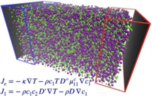
. Shown in Figure is a schematic diagram of the simulation setup together with a snapshot of the system with Kr atoms, in purple, larger in size than Ar atoms, in green.
Figure 1. (a) The subdivision of the simulation box into the different regions, the inner zone, white background, is where the fields and currents are measured, while the regions where the thermostats act on particle velocities are highlighted by different shades of blue for the lower temperature , on the left, and red for the higher temperature
, on the right, with particle exchanges taking place in the darker zones to fix the concentrations to the values
and
, respectively, as described in the text. Periodic boundary conditions are only applied in the x, y-directions, while in the z-direction the system is confined by repulsive walls, dark grey area, placed at the edges of the box. (b) A snapshot is rendered with VMD [Citation14] from the simulation data with temperature gradient
and molar fraction gradient
between the two reservoirs along the z-axis (blue arrow on-axis compass). Note a separation of Kr species (larger size, purple) particles gathering in the higher temperature region,
, as a result of the imposed concentration gradient. The empty spaces in the z-direction are the regions rarely explored by the particles where the wall potential is highly repulsive.
![Figure 1. (a) The subdivision of the simulation box into the different regions, the inner zone, white background, is where the fields and currents are measured, while the regions where the thermostats act on particle velocities are highlighted by different shades of blue for the lower temperature TC, on the left, and red for the higher temperature TH, on the right, with particle exchanges taking place in the darker zones to fix the concentrations to the values x1C and x1H, respectively, as described in the text. Periodic boundary conditions are only applied in the x, y-directions, while in the z-direction the system is confined by repulsive walls, dark grey area, placed at the edges of the box. (b) A snapshot is rendered with VMD [Citation14] from the simulation data with temperature gradient ∇T>0 and molar fraction gradient ∇x1>0 between the two reservoirs along the z-axis (blue arrow on-axis compass). Note a separation of Kr species (larger size, purple) particles gathering in the higher temperature region, TH, as a result of the imposed concentration gradient. The empty spaces in the z-direction are the regions rarely explored by the particles where the wall potential is highly repulsive.](/cms/asset/611d6d50-1546-406e-8199-a4a4aa8b6d92/tmph_a_1892849_f0001_oc.jpg)
All simulations are performed with a fixed total number of particles, on average with a 50/50 split of Ar to Kr atoms. The initial configuration is created by randomly assigning 7056 Ar and 7056 Kr particles with equal probability to the sites of an fcc lattice. After the particles have been placed and their identities assigned, the system is equilibrated by running a 200,000 ts constant temperature dynamics by means of the standard velocity Verlet algorithm coupled to an Andersen thermostat, where random velocity sampling takes place with a 10 ts frequency.
Thermal and concentration gradients are applied to the system in the BD-NEMD production runs. This is accomplished by first removing for convenience two small regions of width at the edges, most of the time empty of particles, and splitting the remaining volume, which is of dimension
, along the z-axis into two reservoir regions at the edges and a central ‘bulk’ region where particles dynamics is not perturbed, but simply determined by the forces arising from intermolecular interactions and following Newton's equations of motion. Each of these regions is split into slices of width
, with constant volume
in reduced units. The two reservoir regions consist of 6 slices at both edges while the bulk region consists of 24 such slices in total, and in each slice the temperature, partial density and energy fields, together with their related currents are calculated at each time step.
In the reservoir regions, temperature and concentration can be imposed individually in each of the 6 slices on both sides of the simulation box. Temperature control is achieved by rescaling the kinetic energy separately for each atomic type.
Concentration control is achieved by a switch of particle identity at random in the reservoir, from Ar to Kr or vice versa, with mass changing while keeping fixed the momentum value, in such a way to attain within ±1 particle the desired concentration value. The origin of the latter limitation in the ability of fixing the concentration is simply due to the fact that the particle count in the reservoir slices cannot be a fractional number. Consider in particular the case of equal concentrations: it can be enforced only if the total number of particles in the slice is even. If this number happens to be odd choosing the type of the last unpaired particle will introduce an excess of one particle type. In the general case of arbitrary concentration, the chosen value to enforce will always fall between two fractional numbers differing at most by one unit in the integer in the numerator: the algorithm will then assign the unknown type for such last remaining particle at random with a probability equal to the desired concentration value. In this way, the concentration in each reservoir slice will asymptotically attain the desired imposed value on average.
In the production run, the 6 slices of each reservoir region are further split into two groups. While temperature control is applied in all the 6 slices, concentration control is only applied to the outermost, with respect to the bulk, 3 slices. This permits having a thermostatted buffer region of width equal to the potential cut-off distance between the fixed concentration reservoirs and the bulk region in which no particle swap takes place. The single-step switch of the particle identity does, in fact, introduce a numerical noise in the integration algorithm, particularly in the case of the smaller Ar to larger Kr transformation where a spike in the force value can result in poor integration of the dynamics at fixed timestep value. Fortunately for the Ar/Kr swap, the differences between the LJ potential parameters are small and with the imposed constant kinetic energy temperature control this problem is minimised. We found that avoiding direct contact between the concentration reservoirs and the bulk region is sufficient to obtain the desired accuracy in the dynamics of the total system. We did observe that without temperature control numerical errors introduced by the sudden particle identity switches, although very small for Ar/Kr on the local scale, results in an unwanted and sizeable overall temperature rise on the very long time scales required to get accurate averages, persisting even over several millions timesteps.
The thermostat regions are dubbed and are outlined in red(right)/blue(left) in Figure . To impose a temperature gradient we set
and
. This establishes a constant thermal gradient with a value very close to
around the mean system temperature
across the inner 24 slices of width
.
Velocity rescaling is performed following a similar procedure to the one outlined in a previous paper [Citation15], where at each timestep, in every thermostatted slice, the total kinetic energy of the individual particle types are calculated after removing the group centre of mass motion from the individual particle velocity. Temperature control is performed in such a way that, individually for each particle type and as a result also globally, the total momentum in each slice is kept unchanged by the velocity rescaling procedure. The scaling factor is determined according to the instantaneous temperature for species
computed from the kinetic energy (
) of the
particles of species
, with
for species 1 or
for species 2. Locally for each slice:
(2)
(2) with
(3)
(3) where
is the instantaneous centre of mass velocity of particles of species
is the instantaneous individual particle momentum and the index i runs over the
particles within the inspected slice. We observed on the very long time scale of our simulations, particularly for the
cases, that thermostats using a velocity rescaling algorithm have a tendency to return a local temperature slightly above the desired value in the bulk region. The difference remains indeed small, below
parts, and it is hardly visible with respect to the statistical noise in the local averages even after averaging over several tens of million timesteps. This shift in temperature effect does not change the temperature gradient as it is constant across the bulk and we ignore its effect. All the values reported for temperature and concentration gradients, as well used in the calculation of transport properties, are those effectively measured by averaging over the particles in the bulk region.
All calculations were performed at fixed zero total momentum for the simulated system in the x- and y-directions, while the component in the z-direction fluctuates around zero only due to the interaction with the containing walls, since the two combined procedures leave the momentum unchanged at each time step. We choose to impose temperature gradients and concentration gradients in the ranges and
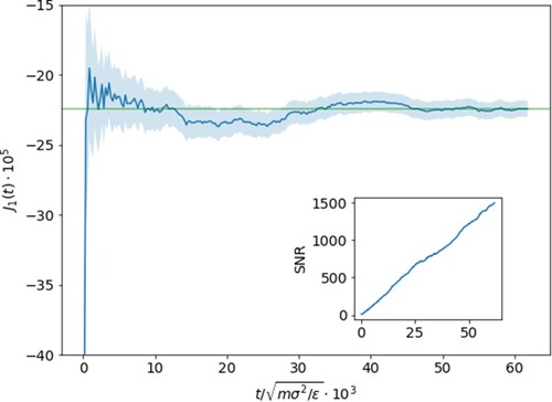
, where each simulation is run for several tens of million timesteps. Long equilibration times are needed to reach stationary flux values and are on the order of
LJ time units as shown in Figure by plotting the running average of the mass flux with (
).
Figure 2. Running average of the mass flux for with error shown by the shaded region. Relaxation to the stationary value occurs after
units with minor long-living fluctuations around the mean value afterwards as shown by the horizontal green line. Shown in the inset is the signal-to-noise (
) ratio which encouragingly continues to steadily climb with increasing statistics.
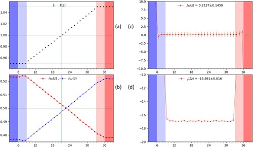
From the simulations, we extract the particle count, mass flux, heat flux, and temperature at each timestep and coarse grain them by averaging in each of the slices over 200 timesteps. The typical coarse-grained result along the z-dimension from a single simulation run are shown in Figure for the case , corresponding (see Section 4) to
in the bulk region. The darker colours at the edges in the panel highlight the different reservoir regions with the adjoining slightly lighter colours indicating the additional thermostat slices.
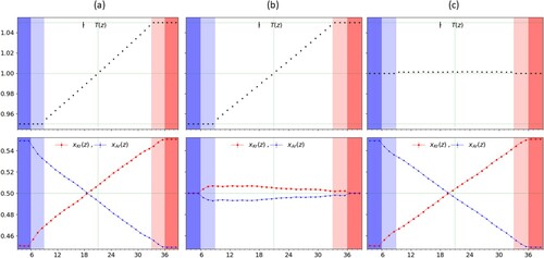
Figure 3. A plot of the temperature (a), mol fraction (b), mass flux of Kr (c), and energy flux (d) as a function of position along the z-direction measured in units of slice width, i.e. , with
. Each point represents the average over a slice and
are indicated by the red(right)/blue(left) shaded regions. The reservoir region in which the mol fraction is controlled consists of only the first and last 3 slices in
as described in the text and are shaded darker. The values reported in (c) and (d) are for the flux averaged across the entire bulk region, neglecting the slices in direct contact with the thermostats and where the faint green line shows the zero level. The vertical green lines in panels (a) and (b) show the equidistant point in the bulk from the reservoirs and it may be observed that the concentration profile (b) is not symmetric in shape for the two species across the bulk and indicates a preference of the heavier Kr towards the colder regions.
3. Theory
The mass and energy flux drive the evolution of a system and the Onsager transport coefficients, notably ,
, and
, measure the strength of the response to imposed gradients. Note that, due to the Curie principle, viscosity belongs to independent transport equations and we will not be concerned with it in the present manuscript. It should be highlighted that these coefficients are only meaningful in the linear regime for which they are derived, where it has been assumed that the system is only at the first-order expansion away from equilibrium. Outside of this regime, the higher orders of the gradients become relevant and need to be considered explicitly.
For a binary system, one can write the constitutive relationships, Equation (Equation1(1)
(1) ), relating these coefficients and the gradients to the energy and mass flux. Microscopically, spatial variations in the chemical potential and temperature are what drive this evolution and give rise to non-zero fluxes. The relevant chemical potential of the system (
with
, respectively, the chemical potential of Kr and Ar, defined per unit mass) is taken to be a function of temperature, pressure, and the molar fraction of component
, i.e.
. We can exploit the fact that in the linear regime the average temperature and pressure remain constant and use Gibbs–Duhem and chain rule (see Appendix) to write
. We choose to take the specific constitutive relations from equation (229) and (230) on page 276 of chapter XI of de Groot–Mazur book [Citation12] expressed in terms of the molar fraction
in the following format:
(4)
(4)
(5)
(5) where
is the mass flux of Kr,
the heat flux,
the partial derivative of the Kr chemical potential at constant temperature and pressure,
the mass density with
the number density,
the mole fraction of Kr, and
the mole fraction of Ar. Onsager reciprocal relations express the equality of the cross coefficients and relate the mass flow induced by a temperature gradient to the energy flux coming from a concentration gradient and manifest itself in the above equations by setting
.
To estimate the heat flux in Equation (Equation4(4)
(4) ) for a given slice we can use equivalently, as shown by Ercole et al. [Citation16], the energy flux defined by Irving and Kirkwood [Citation17] as
(6)
(6) where
is the sum of potential and kinetic energy,
the velocity for atom
,
the barycentric velocity of the tagged slice,
the force on atom
from atom
, and
the vector joining the positions of atom
and atom
. Note that index
extends to particles outside the slice with the slice volume given by
.
We estimate the mass flux in Equation (Equation5(5)
(5) ) by summation of the species momentum in each slice
(7)
(7) where
is the momentum of Kr atoms in slice
. By definition
. The choice of the fixed repulsive wall at the edges permits the system to remain immobile and allows the total momentum to fluctuate, throughout the simulation run, around the initial zero value. We specifically choose to impose along the z-direction confining walls rather than periodic boundary conditions as with the latter, we observed a permanent non-zero barycentric mass flow in the central bulk region compensated by an overall opposite flux created in the two reservoir regions since they are in direct contact through the periodic boundaries. This would contradict the hypothesis of zero bulk barycentric mass flow under which de Groot–Mazur's equations were derived. Finally, we choose to present the results in terms of the heavier particle 1 (Kr), note that only the sign of the Soret coefficient
would change if referring to Ar.
We make in passing the remark that an additional way to write the constitutive relations has been formulated by Trimble and Deutch [Citation18] and followed, not completely consistently, by other studies for transport coefficients [Citation7, Citation15]. This results in defining the coefficients in a slightly different notation. However, conversion between the two can be found and is presented in the Appendix. Note that for the purpose of this manuscript, we present the results using Equations (Equation4(4)
(4) ) and (Equation5
(5)
(5) ), following de Groot–Mazur formalism.
In order for the theory to be correctly applied, there are two requirements that must be fulfilled, first that the system reaches an asymptotic state in which the fluxes reach a uniform stationary value across the central bulk region and second that the strength of the imposed gradients remains in the linear regime region. Once that is assessed, we also need to make a proper estimate of the errors associated with the statistical averages, which provide the values of the fluxes. We can postpone to the next section the checks for both requirements, while we conclude this section discussing the algorithm we will use to evaluate the errors.
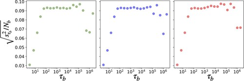
We remind that values sampled along a trajectory generated by Molecular Dynamics are often correlated in time and for error analysis we need to estimate correctly the number of independent contributions to the averages. The error associated to the flux value is computed via a block averaging approach which allows for independent samples to be obtained by uniformly partitioning the trajectory into different blocks, giving blocks of equal length
, as described in Flyvbjerg and Petersen [Citation19]. The
necessary to determine when the independence of block averages occurs is taken through observation of when the estimated variance of the block averages of length
divided by
reaches a plateau. An example of this procedure is shown in Figure . The error of the overall average is then computed through the following set of equations:
(8)
(8)
(9)
(9)
(10)
(10)
(11)
(11) where
is either the mass or energy flux value at an instant i in time within the particular time block b,
is the, generally biased, estimate of the variance of
and is a function of the time length
of the blocks. For high frequency sampling rates, the estimate is biased due to the values being correlated in time. The unbiased estimated variance of
is taken as the value of
as a function of
in the range where it remains approximately constant.
Figure 4. The estimated standard deviation for from the block analysis of three independent trajectory segments each of
timesteps for the (
) condition. Values for (
) are plotted against the number of timesteps in each block
, where
is the number of blocks and
. The region between 100 and 10,000 steps shows a relatively flat profile, which implies that there the block averages can be considered as independent samples. Going to shorter intervals of time, the decrease can be traced back to increasing correlations while at the other end the number of blocks
becomes too small to provide a reliable estimate of the variance of the sample.
4. Results
We start by showing that both requirements mentioned in Section 3 are met, namely that the flux values are relaxing to stationary values and that the gradients applied are kept in the linear regime. The relaxation of the mass flux of particle 1 is shown in Figure for the case of . We see that the presence of long-lived fluctuations after an initial ‘fast’ relaxation requires averages over time intervals lasting longer than O(
), but that the value does plateau and promisingly that the signal-to-noise ratio climbs steadily with time, testifying the achievement of asymptotic stationary conditions.
The first check for linearity can be quickly performed by comparing the values of the fluxes with the corresponding gradients when, while keeping , we double the imposed concentration boundary value from
. Resulting in
with
and
with
. Thus giving a ratio of
. We recall that while for the temperature gradient
holds to a high degree of accuracy, this is not the case for the concentration gradient
in the presence of a non-zero temperature gradient in the bulk region. Therefore, the general test for linearity consists in showing that
for any combination of the individual imposed gradients. Results from combining the imposed boundary conditions
, are analysed in Table and show that, with small relative errors, the condition for linearity is well satisfied.
Table 1. Check of linearity using the measured values of the temperature gradient, the energy flux, the molar fraction gradient and the mass flux for component 1, reported in LJ units.
With the requirements for linearity and stationarity of the fluxes and gradients fulfilled, we next move to the calculation of the transport coefficients with the BD-NEMD method. We can see from the constitutive relations, Equations (Equation1(1)
(1) ), that if we impose all but one gradient to be zero, we can measure one by one the elements of the matrix of coefficients while varying the strength of the non-zero gradient. So, at least in principle, in our procedure we have to set one of the two gradients equal to zero to extract directly the two transport relevant coefficients from the ratio of the resultant measured fluxes and the strength of the other gradient. As said, we only impose boundary values, so this is possible only after ensuring that the observed value of the first gradient is actually close to zero in the central bulk region ; otherwise, the residual value of the non-vanishing gradient needs to be taken into account explicitly. However, while we can impose the condition
with any desired degree of accuracy, in the presence of a non-zero temperature gradient a nonnegligible molar fraction gradient
is unavoidable in the bulk region. Therefore we start by extracting the transport coefficients from Equations (Equation4
(4)
(4) ) and (Equation5
(5)
(5) ) in the case when
and
. With both
and
known, the binary diffusion coefficient D and the product
can be computed by rearranging the two equations to give
(12)
(12)
(13)
(13) The gradients
and
are the ones calculated from the temperature and molar fraction profiles in the bulk region between
to
, as shown in Figure (c) for the case
and
. We can observe that the corresponding temperature profile is indeed flat, satisfying the condition
. One can see that in the bulk region, there is a slight temperature increase with respect to the reservoir regions, but it remains uniform and therefore gives no contribution to the flux so that D and the product
can be readily estimated from the above equations.
Figure 5. The temperature (top) and concentration (bottom) profiles where panels (a), (b) and (c) are for conditions respectively. Each point represents the average over a slice and regions
are indicated by the red(right)/blue(left) shaded areas. The reservoir region in which the mol fraction is controlled consists of only the first and last 3 slices in
as described in the text and are shaded darker. From (b), one can see that while the concentration is equal at both edges, it is not enough to force the profile in the bulk to be uniform and a small gradient emerges, with opposite sign to the temperature gradient.
We next impose the conditions in order to obtain the heat conductivity κ and the thermal diffusion coefficient
. However, in this case, as it can be observed from Figure (b) for
, a residual, stationary, non-zero gradient in concentration is present in bulk region, despite the imposed equimolar ratio in the reservoirs, and its contribution to the mass flux of component 1 cannot be ignored. Thus in order to compute the latter two transport coefficients correctly we need to account for both the temperature and the concentration gradients from the observed profiles Figure (b) and plug their values in the following expressions for κ and
, derived again from Equations (Equation4
(4)
(4) ) and (Equation5
(5)
(5) ):
(14)
(14)
(15)
(15) Summarising, from the simulation with
an accurate computation of
and the product
can be performed. Then these results can be used in a second simulation with
to complete the calculation of all coefficients for the remaining values of
and κ. Note that also
can now be computed.
With the flux values and necessary profiles in hand and following the procedure outlined above, we recollect the transport coefficients from the present study in Table .
Table 2. Heat and mass transport coefficients from the BD-NEMD protocol.
This numbers, reported to the Onsager coefficients, are compared in Table with those calculated by Sarman and Evans [Citation2], where the coefficients were extracted from Green-Kubo relations for a system of Ar–Kr using the Evans–Cummings scheme [Citation20], an algorithm to drive NEMD simulations by equating the time derivative of the Hamiltonian to a product of the flux and a mechanical force which gives the exact Green-Kubo relations in the linear limit.
Table 3. Comparison of the Onsager coefficients between our results (BD-NEMD) and those from the mechanical perturbation scheme by Sarman and Evans [Citation2] for a system of 1024 particles of Ar-Kr.
Rather than the values of the transport coefficients and of
, which are not calculated directly in the mechanical perturbation scheme, we compare with the values of the Onsager coefficients
and
calculated from our data (see Appendix for the details of definitions).
We see relative agreement between the two methods despite a small difference in our thermodynamic points and it should also be considered that the Sarman and Evans results were obtained with less statistics and for smaller system size.
As a further check of the new method, we also compare the Soret coefficient defined as [Citation12] with the one computed using the protocol following studies used in [Citation5, Citation15], which consists of imposing a temperature gradient at the edges of the simulation box and allowing the system to relax to mass equilibrium by the establishment of a natural concentration gradient. When
, the Soret coefficient can be taken as the ratio of the observed concentration gradient over the observed thermal gradient [Citation12], i.e.
.
We explored the behaviour of our system resulting from the imposition of only the difference in temperature between the two reservoir regions in order to estimate the naturally occurring concentration gradient. In practice, we found that the relaxation time needed to establish the asymptotic concentration and temperature profiles, i.e. to achieve mass equilibrium in the central bulk region, can be exceedingly long and that, correspondingly, the average mass flux remains small but non-zero even after very long times, reaching a final value that, divided by a number of the same order of magnitude (the product of the binary diffusion coefficient and thermal gradient) lead to an important correction for
, as we now show.
Making use of the binary diffusion coefficient D measured with the BD-NEMD scheme, we take the residual value of into account to obtain the improved expression
(16)
(16) and use it to compute the Soret coefficient using the gradients in two equivalent
conditions. In fact, thanks to the ability to fix both the concentration and the temperature in the reservoirs to our liking, we can pursue an alternative route to establish the same stationary flux
in a driven condition by imposing at the same time as
an appropriate boundary value for the concentration,
. Comparison of the gradients and fluxes obtained with these two alternative routes is summarised in Table . Both setups show a similar deviation from zero mass flux,
in one case and
in the other, so that, after treatment, both give
.
Table 4. Results of the measured fluxes and gradients in the bulk for the experimentally inspired protocol where .
Indeed, the values from Table give for two nonconsistent values, that is 1.747 (0.003) when we drive the system imposing both gradients and 1.644 (0.003) when we allow the system to reach the mass equilibrium state in the presence of a temperature gradient alone. Consistency is regained with Equation (Equation16
(16)
(16) ) including the correction due to the non-zero mass flux, as shown in Table . In this way, we do also get a consistent agreement with the value
previously calculated from the transport coefficients from BD-NEMD.
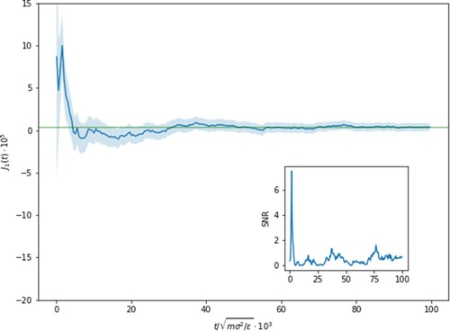
In Figure , we show the behaviour of the running average of in the driven condition. We can see that even after
LJ-units, the average mass flux is small but non-zero, reaching a final value (
) and that frustratingly the error associated with it is not insignificant in comparison (
). The increased uncertainty in the value of the Soret coefficient calculated from Equation (Equation16
(16)
(16) ) stems from such non negligible error associated to the evaluation of
as highlighted in the inset of Figure .
Figure 6. Running average of the mass flux with the shaded region showcasing the error with and
to achieve mass equilibrium. Note that even after
, there is still a measurable mass flux value and that at
the uncertainty is as large as the signal. This is shown more prominently in the inset where the signal-to-noise is given over time and contrasting to the inset of Figure where the SNR rose monotonically with simulation time.
Note that we showed that not considering the second term with results in underestimating the error on the value of
. While it has been reported that the Soret coefficient has an extreme sensitivity to even a minor perturbation in the imposed gradient, our results point rather to the large uncertainties on
coming from the difficulty to achieve the condition
with sufficient accuracy to justify neglecting its value. If this factor cannot be safely ignored, then knowledge of the binary diffusion coefficient must be obtained. In this respect, the benefit of the new BD-NEMD technique becomes apparent in that we can derive the value of the Soret coefficient directly from
computing the two transport coefficients in stationary non-equilibrium conditions, with an accuracy that can be improved at will by increasing the statistics or exploring in the linear regime a range of gradients conditions that can be plotted against the fluxes and the coefficients found through a simple linear fitting procedure.
5. Discussion
In the present manuscript, we have introduced a method that permits to set at will both a concentration and a temperature linear gradient by imposing simultaneously appropriate conditions at the edges of the simulation box and we used it to make a direct simulation of transport processes. The method has been applied here to binary mixtures but it can be straightforwardly generalised to multicomponent systems.
These are moreover real thermodynamics forces as opposed to the mechanical perturbations used by Evans et al. [Citation2, Citation3]. The bulk region in between the edges is run with Newtonian dynamics and it is from this bulk that we can obtain stationary mass and energy flux values, varying the imposed temperature or concentration gradients while keeping the other gradient fixed to zero. This gives the desired transport coefficients using the constitutive relations presented by de Groot–Mazur and valid in the linear regime. We compare the results for to the one obtained by running with a protocol where the system establishes a mass equilibrium by creating a concentration gradient countering the temperature polarisation of the system so that
. The two methods give consistent results, but to get complete alignment we need to consider the explicit residual value of
from this setup even for apparently very small order of magnitudes in order to correctly determine the uncertainty. Because of this, two other benefits of running the new BD-NEMD technique over this protocol are that (i) because no flux signal is perfectly zero, the stationary values give a higher signal-to-noise ratio and (ii) we can explicitly compute all the various transport coefficients and not be constrained to only extract their relative ratios or have to rely on equilibrium sampling techniques. This opens the possibility for exploration into the driving forces for glassy systems or purification where the thermal and concentration gradients are of similar magnitude and it is desired to compute the specific contributions to the magnitude of the flux evolution. Moreover, by fixing one species type and varying the other, this technique allows for a range of transport properties to be determined and thus allows for creation of more suitable mixtures. This is particularly useful in areas involving nanofluids [Citation21] in specific applications like refrigerant cooling where thermal diffusion is thought to play a more significant role and screening possible candidates based on observed properties can be difficult.
We highlight that while the technique is broad and applicable to any system, the results themselves can have a dependence on the thermodynamic point making comparison and estimation for different systems challenging. The results we present are only for a system of moderate packing density () and only for the mild change of Ar to Kr and vice versa. In the future, we plan to explore more dramatic changes such as Na
to K
, as the depolarisation of this specific type of concentration gradient is responsible in biological system signalling [Citation22]. Other avenues include dramatically varying the particle size such as in the separation of polymers. This may require a modification to the current simulation setup as a sudden particle type change in the reservoir regions can lead to instabilities caused by large steric overlap. This could potentially be circumvented by introducing a different time integration scheme in the reservoir regions or by the gradual growing or shrinking as is commonly done in free energy perturbation methods [Citation23–25]. We hope to apply this technique in a wide variety of applications where non-equilibrium states due to imposed gradients can be found and help elucidate the strength of the elusive cross-coefficient terms.
Acknowledgments
We are delighted to dedicate this small contribution in non-equilibrium molecular simulation to Mike Klein who has just achieved his 80 years. We wish he will continue to share with us his human and scientific wisdom for many years to come. This work is supported by grants from the Welch Foundation F-1896 and from the NIH GM059796.
Disclosure statement
No potential conflict of interest was reported by the author(s).
Additional information
Funding
References
- W. Kohler and K.I. Morozov, J. Non-Equilib. Thermodyn. 41 (3), 151–197 (2016). doi:https://doi.org/10.1515/jnet-2016-0024
- S. Sarman and D.J. Evans, Phys. Rev. A 45 (4), 2370–2379 (1992). doi:https://doi.org/10.1103/PhysRevA.45.2370
- S. Sarman and D.J. Evans, Phys. Rev. A 46 (4), 1960–1966 (1992). doi:https://doi.org/10.1103/PhysRevA.46.1960
- B. Hafskjold, T. Ikeshoji and S.K. Ratkje, Mol. Phys. 80, 1389–1412 (1993). doi:https://doi.org/10.1080/00268979300103101
- D. Reith and F. Muller-Plathe, J. Chem. Phys. 112 (5), 2436–2443 (2000). doi:https://doi.org/10.1063/1.480809
- P. Wirnsberger, D. Frenkel and C. Dellago, J. Chem. Phys. 143 (12), 124104 (2015). doi:https://doi.org/10.1063/1.4931597
- M. Ferrario, S. Bonella and G. Ciccotti, Eur. Phys. J.-Spec. Top. 225 (8–9), 1629–1642 (2016). doi:https://doi.org/10.1140/epjst/e2016-60137-4
- B. Hafskjold, Eur. Phys. J. E 40 (1), 539 (2017). doi:https://doi.org/10.1140/epje/i2017-11492-9
- V. Vaibhav, J. Horbach and P. Chaudhuri, Phys. Rev. E 101 (2), 539 (2020). doi:https://doi.org/10.1103/PhysRevE.101.022605
- S. Hollinger and M. Lucke, Phys. Rev. E 52 (1), 642–657 (1995). doi:https://doi.org/10.1103/PhysRevE.52.642
- R.L. Rowley and F.H. Horne, J. Chem. Phys. 72 (1), 131–139 (1980). doi:https://doi.org/10.1063/1.438897
- S.R. De Groot and P. MazurNon-equilibrium Thermodynamics (Dover Publications, New York, 2013).
- J.N. Israelachvili, Intermolecular and Surface Forces (Academic Press, Amsterdam, 2011).
- W. Humphrey, A. Dalke and K. Schulten, J. Mol. Graph. 14, 33–38 (1996). doi:https://doi.org/10.1016/0263-7855(96)00018-5
- S. Bonella, M. Ferrario and G. Ciccotti, Langmuir 33 (42), 11281–11290 (2017). doi:https://doi.org/10.1021/acs.langmuir.7b02565
- L. Ercole, A. Marcolongo, P. Umari and S. Baroni, J. Low Temp. Phys. 185 (1–2), 79–86 (2016). doi:https://doi.org/10.1007/s10909-016-1617-6
- J. Irving and J.G. Kirkwood, J. Chem. Phys 18, 817–829 (1950). doi:https://doi.org/10.1063/1.1747782
- R. Trimble and J. Deutch, J. Stat. Phys. 3 (2), 149–169 (1971). doi:https://doi.org/10.1007/BF01019848
- H. Flyvbjerg and H.G. Petersen, J. Chem. Phys. 91 (1), 461–466 (1989). doi:https://doi.org/10.1063/1.457480
- D.J. Evans and P.T. Cummings, Mol. Phys. 72, 893–898 (1991). doi:https://doi.org/10.1080/00268979100100621
- E.E. Michaelides, J. Non-Equilib. Thermodyn. 38 (1), 1–79 (2013). doi:https://doi.org/10.1515/jnetdy-2012-0023
- M.J.V. Clausen and H. Poulsen, in Metallomics and the Cell. Metal Ions in Life Sciences, edited by L. Banci, Vol. 12 (Springer, Berlin, 2013), pp. 41–67.
- C. Chipot and A. Pohorille, editors, Free Energy Calculations (Springer, Berlin, 2007).
- T. Lelièvre, M. Rousset and G. Stoltz, Free Energy Computations (Imperial College Press, London, 2010).
- A. Fathizadeh and R. Elber, J. Chem. Phys. 149 (7), 072325 (2018). doi:https://doi.org/10.1063/1.5027078
- L. Onsager, Phys. Rev. 37, 405–426 (1931). doi:https://doi.org/10.1103/PhysRev.37.405
Appendix. Reconciling Trimble–Deutch to de Groot–Mazur
In the present manuscript, we attempted to make comparisons primarily to the results in [Citation3, Citation7, Citation15]. However, we found that the coefficients defined in the constitutive equations in [Citation18] relating the flux to the transport equations do not match properly the ones given by de Groot and Mazur [Citation12]. We know that Onsager relations state that the mass flow per unit of imposed temperature difference should be equivalent to the energy flow per unit of imposed concentration gradient [Citation26]. Under the assumption of microscopic reversibility this means that the cross coefficients , when defined with respect to the thermodynamic forces
, should be identical. However, with the introduction of additional coefficients in the equations that is not immediately evident.
We first start by recalling the constitutive relations for a binary system in equations (212 and 213) from page 274 in Chapter XI of Non-Equilibrium Thermodynamics [Citation12]. In order to simplify the comparison with the corresponding expressions of Trimble and Deutch [Citation18], without having to include too many additional constant conversion factors that can ultimately hide the important part of the result, we choose here to follow de Groot–Mazur to work, rather than with the previously used molar fractions, in terms of the mass fractions and
. The relation within the two alternative descriptions if fully given in Chapter XI of [Citation12]. For a binary system the relevant chemical potential appearing in the expression of the thermodynamic force
driving mutual diffusion is given by
where
and
are the specific chemical potential of components 1 and 2, respectively, and at constant
and
satisfy the Gibbs–Duhem relation
. The following expression for the gradient of μ at constant temperature in terms of the gradient of the mass fraction
,
can then be derived, introducing here for brevity the quantity
. Note that the quantity
introduced in Section 3 is the equivalent abbreviation when using
as a function of the molar fraction
rather than of the mass fraction
. We can transform from one to the other by means of the relation
, that can be easily derived from the above definition of
and
.
The transport coefficients and
are then defined
(A1)
(A1)
(A2)
(A2) and showed to satisfy the equality
as a result of Onsager relation
. The superscripts
has been used here to identify the quantities defined using the formalism of de Groot-Mazur, while the superscript
will be used in the following to distinguish similar, but somehow differing, quantities defined in Trimble and Deutch formalism. In equations (90) and (91) on page 167 of Trimble and Deutch [Citation18] the Onsager relation is imposed in terms of somewhat different phenomenological coefficients
and the equations are then recast defining different transport coefficients
:
(A3)
(A3)
(A4)
(A4) Finally, by comparing, term by term, the expressions in front of the imposed gradients in Equations (EquationA1
(A1)
(A1) ) and (EquationA2
(A2)
(A2) ) with those in Equations (EquationA3
(A3)
(A3) ) and (EquationA4
(A4)
(A4) ) the conversion between the two formalisms can be fully expressed as
(A5)
(A5)
(A6)
(A6)
(A7)
(A7) resulting in the following alternative expressions for the Soret Coefficient
(A8)
(A8) Note finally that, following de Groot and Mazur [Citation12], for the case
the more commonly used expression for
can be derived from Equation (EquationA2
(A2)
(A2) )
(A9)
(A9)
where the right-hand side, in terms of molar fractions, is the actual expression we used when discussing our results in Section 4 and follows immediately by means of the equality
.