Effect of social distancing on super-spreading diseases: why pandemics modelling is more challenging than molecular simulation

Abstract

This paper aims to present some features of the non-Poissonian statistics of the spread of a disease like COVID19 to a community of chemical-physicists, who are more used to particle-based models. We highlight some of the reasons why creating a ‘transferable’ model for an epidemic is harder than creating a transferable model for molecular simulations. We describe a simple model to illustrate the large effect of decreasing the number of social contacts on the suppression of outbreaks of an infectious disease. Although we do not aim to model the COVID19 pandemic, we choose model parameter values that are not unrealistic for COVID19. We hope to provide some intuitive insight in the role of social distancing. As our calculations are almost analytical, they allow us to understand some of the key factors influencing the spread of a disease. We argue that social distancing is particularly powerful for diseases that have a fat tail in the number of infected persons per primary case. Our results illustrate that a ‘bad’ feature of the COVID19 pandemic, namely that super-spreading events are important for its spread, could make it particularly sensitive to truncating the number of social contacts.

GRAPHICAL ABSTRACT

Keywords:

• Pandemic
• generating function
• social distancing

1. Introduction

Like weather prediction, real-time modelling of a pandemic, whilst imperfect and unreliable for long-term predictions, is clearly indispensable for assessing mitigation strategies. During the 2020/2021 outbreak of COVID19, there has been explosive growth in pandemic-modelling studies. At present, the state-of-the-art models of the COVID19 pandemic are highly sophisticated, stratified and heterogeneous. Often, in analogy with molecular simulations, some of the advanced models are agent-based, with as many ‘agents’ as there are humans in a given population. However, as with simulations, it is not always easy to correlate the outcome of complex model calculations with the values of the very large number of individual input parameters. This is why simple models that depend on only a few parameters are still important.

In what follows, we discuss such a simple model. It is different from the better known SEIR (Susceptible-Exposed-Infected-Removed)-model and its many, often quite sophisticated [1], variants: ‘Removed’ stands for ‘Recovered’ but also includes the less pleasant option that the infected person does not recover. SEIR models typically are based on a set of coupled, nonlinear differential equations, often with some stochasticity. However, these equations treat the number of infected persons as a continuous variable, which could be less than one and then grow again. In practice, of course, if the number of infected person drops below one, that particular outbreak stops.

The discreteness of the spread of pandemics is taken into account in agent-based models of the pandemic or, as they are called in the field, Individual-Based Models (IBMs). Here, the discreteness is taken into account from the very beginning, but the calculations – like particle-based simulations in the physical sciences – are expensive. Moreover, each agent can have ‘attributes’: age, gender, ethnicity, size of household, pre-existing conditions, time since infection, travel patterns, etc. These attributes make IBMs very powerful, but interpreting the sensitivity of the model-outcomes to the values of the different attributes can be very demanding.

The very simple model that we use here for early-stage outbreaks is simpler even than the simplest SEIR models, but it retains one key feature of the IBMs: the number of infected persons must be an integer.

We stress that the level of modelling that we use would be considered embarrassingly simplistic by epidemiologists. However, it may help clarify some concepts in the control of epidemics for those of us who are more familiar with molecular modelling.

2. Motivation

One of the disconcerting aspects of the COVID19 pandemic is that in many countries it could stay undetected for relatively long periods of time, before the exponential growth phase became visible, as measured, grimly but reliably, by the excess number of deaths. Of course, even with exponential growth from a single case, it is to be expected that an outbreak will initially be ‘under the radar’, but there is evidence that the large-scale outbreak in various countries were preceded by relatively long periods when the disease was apparently present, but not growing rapidly. This puzzling behaviour has even led to some to postulate that a sizeable fraction of the population is effectively immune without having been exposed to SARS-CoV2 [2].

It seems likely that in some regions, the disease was introduced multiple times but that most of these introductions did not result in an outbreak. The question then arises how many ‘failed’ outbreaks (on average) preceded the real outbreak.

Answering this question may also be important for understanding the curious spread of the disease, which in many countries seemed to show initially (sometimes for many months) a remarkably non-uniform spatial distribution. Yet, as time progressed (from the first wave to the second wave), the distribution became more homogeneous, both in the USA and in various European countries.

Such behaviour would also be expected if the disease had been introduced numerous times in these low-incidence regions, but then petered out. The steady sequence of transients might give the impression of an epidemic that did not grow, but in the scenario of repeated reintroduction of the disease, the constant level of infections would simply be due to a steady ‘drip’ of new infections, possibly followed by small outbreaks due to local super-spreading events, which did not lead to a sustained larger-scale outbreak.

In this paper, we try to estimate the probability that a single infection in a susceptible population will not lead to an outbreak.

Here, we immediately run into the problem faced by all groups carrying out large-scale model simulations: what are the correct parameters required to characterise the growth of the pandemic? After more than a year of news coverage, the concept of the bare reproduction number $R_0$ seems to be sufficiently widely known that it is mentioned without further explanation in news reports – sometimes as if it is an intrinsic property of the virus, which it is not – or, at least, not exclusively. $R_0$ is the average number of secondary infections caused by a single infected individual in the absence of any interventions to suppress the spread of the disease.

Clearly, $R_0$ depends on the nature of the pathogen: the original strain of COVID19 seemed to have a reproduction number that is about an order of magnitude less than that for the measles. But $R_0$ also depends on many social and environmental factors. So much so that, even in the absence of interventions, one should not assume $R_0$ to be constant in either space, time or across different communities. In fact, this is why more realistic models must take societal heterogeneity into account [3].

To complicate matters more, the number of people infected by a single carrier is not Poisson-distributed, i.e. the probability to find n secondary cases is not equal to $(R^n/n!)\exp (-R)$; here, and in what follows, we drop the subscript 0 of $R_0$ unless explicitly stated otherwise. Rather, the real probability distribution of the number of secondary cases seems to have a much larger dispersion than the Poisson distribution. Such an over-dispersion means that the variance in the number of secondary infections can be much larger than the average; for a Poisson distribution, these two numbers would be equal. A symptom of this over-dispersion is the fact that most infected persons infect nobody at all, even when R is large. In fact, there is considerable evidence that less than 20% of all cases account for around 80% of all secondary infections [4] (for SARS, comparative data have been published: [5]).

3. Negative binomial distribution

A central quantity in the description of an outbreak is the probability distribution that a single infectious person will infect n secondary cases. We will denote this probability distribution by $p(n,1;\mathrm{\Delta }t)$, where $\mathrm{\Delta }t$ denotes the length of a single generation interval. As we will keep $\mathrm{\Delta }t$ constant, we leave it out in what follows and write $p(n,1)$ for the distribution of secondary cases infected by one person in one generation interval of length $\mathrm{\Delta }t$.

In the case of COVID19, the distribution of secondary cases is often assumed to be well described by the so-called negative-binomial distribution (the name can be explained, but the explanation does not clarify much), which depends on R and on a parameter k, quantifying the degree of over-dispersion. The negative-binomial expression for the probability density $p(n,1)$ of the number of secondary infections n, is given by (1) $p(n,1)=\frac{\mathrm{\Gamma }(n+k)}{n!\mathrm{\Gamma }(k)}{\left(\frac{k}{k+R}\right)}^k{\left(\frac{R}{k+R}\right)}^n,$(1) where Γ denotes the gamma function. The average number of secondary cases predicted by this negative-binomial distribution is R, as it should. The variance in n is given by $R(1+R/k)$. Well-known limits of the negative-binomial distribution are the Poisson distribution, when $k\to \mathrm{\infty }$, and the geometric distribution when k = 1. 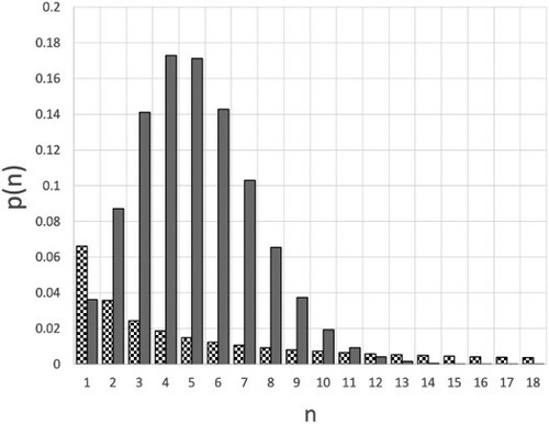Note that for $k\ll 1,$ the dispersion of the number of secondary cases can be much larger than R, in other words, the distribution of secondary case numbers has a ‘fat tail’ [6]; some preprints on COVID19, based on limited data, even suggested very fat ‘power-law’ tails [7]. The large difference between Poisson distribution and the over-dispersed negative binomial distribution is shown in Figure 1, which compares the Poisson distribution for R = 5 with the negative binomial distribution for k = 0.1. The values for $p(0,1)$, the probability that one person infects nobody else, are not shown in the plot because this value would dominate the plot in the case of small k: for the Poisson case, $p(0,1)\approx 0.0067$, whereas for the case with k = 0.1, $p(0,1)\approx 0.67$. Typical estimates for k for the case of COVID19 are in the range between 0.1 and 0.2 [9,10], but probably closer to 0.1. Estimates for R are scattered (fairly widely) around 2.8 for the original strand of the SARS-CoV2 virus, but for the variants that appeared in late 2020, it may be as high as 4 (if not higher) [8].

Figure 1. Comparison of the probability distribution $p(n,1)$ for a value of R = 5, which is in the range of the COVID19 variants that appeared in late 2020 [8]. The grey bars correspond to a Poisson distribution; the chequered bars correspond to a negative binomial with k = 0.1. To improve the readability of the figure, the data points for n = 0 have not been included. For the Poisson case, $p(0)\approx 0.0067$, whereas for the case with k = 0.1, $p(0,1)\approx 0.67$, which means that 67% of all infectious persons infect nobody else.

Low values of k are typical for infections whose spread is strongly influenced by super-spreader events: events with a high value of n that, whilst rare, nevertheless make a significant contribution to R. In fact, for small values of k, an increase in R has little influence on the probability to infect only a few other individuals: most of the difference is in the tail of the distribution (see Figure S1 of ref. [11]).

Interventions such as physical distancing, tracing and isolation of contacts, and lockdowns, result in an apparent increase in k. We will not follow this approach. Rather we will assume that the main effect of social isolation measures is to introduce an upper cut-off to the number of people that can be infected by a single individual. Such a truncation will, of course, also decrease the effective reproduction number, provided that we keep the parameter R constant. The idea of ‘chopping the tail’ of the distribution has recently been highlighted by other authors [12,13].

Our aim is to show how this effect can be understood using a very simple model. It is obvious that truncation affects the effective value of R: (2) $R_{\mathrm{eff}}=\sum _{n=1}^{n_t}{p}^{\mathrm{\prime }}(n,1)n,$(2) where $p^{\mathrm{\prime }}(n,1)$ is the original distribution but now normalised in the range $0\le n\le n_t$. In what follows, we will explore how the probability that a single infected person causes no outbreak, depends on R and k. We will use-values for these parameters that are in line with the available estimates COVID19, but we stress that, in spite of a massive research effort, both numbers are not accurately known and, as we argued above, part of the problem is that they are not constants of nature. Having said that, it is clear that, as more infectious strands of a virus emerge by mutation, R will increase because that is our measure of infectiousness. Much less is known (to our knowledge) about the effect of mutations on k. It seems likely that, as long as the spreading mechanism is not changed (e.g. the relative importance of direct contact and airborne transmission), the value of k is more determined by interaction network of individuals than by the virus. However, one could imagine that if a mutation would increase the survival time of a virus in an aerosol droplet, then k would go down.

4. The transmission matrix

To keep things simple, we will represent the time evolution of the early stages of an outbreak as a discrete Markov process. By considering early stages only, we can ignore the fact that, as the pandemic progresses, an increasing fraction of the population is (at least temporarily) barely susceptible.

A single step in our Markov process represents a single generation interval of the disease, i.e. the average number of days between a specific infection event and a subsequent secondary infection. In reality, there is, of course, a distribution of such times [14].

We next consider the transmission matrix $\mathbf{\text{G}}$. The elements of the matrix $\mathbf{\text{G}}$ give the conditional probability that, if at time t we have m infections, we will have n spawned infections at time t + 1 (the unit of time is the generation interval). As we consider a discrete process with a fixed time interval between subsequent infection events, the elements $G_{nm}$ do not depend explicitly on time, as they would have, if we had considered a continuous-time process. Also, we only consider direct transmission in one-time step. Hence, transmission is a Markov process.

In order to compute the elements of the matrix $\mathbf{\text{G}}$, we need to know the distribution of infections caused by a single infection event, and from that, the distribution of the number of infections at t + 1 caused by m infections at t.

For what follows, it is useful to introduce the generating function (3) $\tilde{p}(s;1)\equiv \sum _{n=0}^{n_t}{p}^{\mathrm{\prime }}(n,1)s^n.$(3) Clearly, the coefficient of $s^n$ in $\tilde{p}(s;1)$ is simply $p^{\mathrm{\prime }}(n,1)$, so we do not really need the generating function here. However, when we consider the probability $p(n,m)$ that m infectious persons will generate n new infections, then the use of generating functions becomes convenient. To see this, consider the probability that there are two infectious persons. What is the probability $G(2,2)$ that they will subsequently infect two others? Clearly, that probability is $p^{\mathrm{\prime }}(2,1)p^{\mathrm{\prime }}(0,1)$ + $p^{\mathrm{\prime }}(1,1)p^{\mathrm{\prime }}(1,1)$+ $p^{\mathrm{\prime }}(0,1)p^{\mathrm{\prime }}(2,1)$. But that is equal to the coefficient of $s^2$ in ${\tilde{p}}^2(s,1)$, In general, if we define (4) $\tilde{p}(s;m)\equiv (\tilde{p}(s;1){)}^m,$(4) then the coefficient of $s^n$ equals $G_{nm}$. Below (see Section 7), we shall also make use of a related matrix $\mathcal{G}(s)$, with as elements ${\mathcal{G}}_{nm}(s)=G_{nm}{s}^n$. Clearly, $G_{nm}={\mathcal{G}}_{nm}(s=1)$. With this notation, (5) $\tilde{p}(s;m)=\sum _{n=0}^{\mathrm{\infty }}{G}_{nm}{s}^n=\sum _{n=0}^{\mathrm{\infty }}\mathcal{G}(s).$(5) We stress that the use generating functions in modelling the spreading of a disease as such is not new [15].

5. Practical implementation

After a sufficiently long time, a single infection will have resulted either in an outbreak, or in just a transient. It is not our aim to model the growth in the number of infections, once this growth is unstoppable. Rather, we consider two scenarios: an initial infection will eventually result in 0 new infections, or in a number N that is larger than $k_{\max }$, where $k_{\max }$ is a threshold value beyond which outbreaks will (almost certainly) grow in the absence of mitigation steps.

In our calculations, we choose $k_{\max }$ sufficiently large that our results for the outbreak extinction probability are not sensitive to the precise value of $k_{\max }$. Typically, a value of $k_{\max }=100$ is large enough.

An outbreak stops once the number of cases has reached n = 0. n = 0 is an absorbing boundary, that is, probability can flow into this state, but it cannot flow out – but that is just a fancy way of saying that the spread stops once there are no infectious cases.

The probability that a state with m cases at t will result in $m^{\prime }$ cases at t + 1 can be computed from the negative-binomial distribution (Equation  (1(1) $p(n,1)=\frac{\mathrm{\Gamma }(n+k)}{n!\mathrm{\Gamma }(k)}{\left(\frac{k}{k+R}\right)}^k{\left(\frac{R}{k+R}\right)}^n,$(1) )).

We now define the generating function for the unnormalised truncated, negative-binomial distribution: (6) ${\tilde{p}}_u^{(t)}(s,1)\equiv \sum _{n=0}^{n_t}\frac{\mathrm{\Gamma }(n+k)}{n!\mathrm{\Gamma }(k)}{\left(\frac{k}{k+R}\right)}^k{\left(\frac{R}{k+R}\right)}^n{s}^n,$(6) where the superscript $(t)$ denotes ‘truncated’ and the subscript u indicates that fact that if we simply zero all $p(n,1)$ with $n>n_t$, then the resulting probability distribution is not normalised. Later (see Section 6), we will discuss different choices to normalise the truncated distribution to obtain a properly normalised $p^{\mathrm{\prime }}(n,1)$ and from that ${\tilde{p}}^{(t)}(s,1)$. Below, we will take an advance on Section 6 and assume that we have carried out this normalisation.

It is convenient to choose s complex, because in that case we can compute ${\tilde{p}}^{(t)}(s,1)$ from $p(n,1)$ by discrete Fourier transform, and ${\tilde{p}}^{(t)}(s,m)=({\tilde{p}}^{(t)}(s,1){)}^m$. We can then obtain all elements of the matrix $\mathbf{\text{G}}$ by inverse Fourier transform. In particular, $G_{nm}$ is the coefficient of $s^n$ in ${\tilde{p}}^{(t)}(s,m)$.

With this information, we can compute the probability that a state with m infected individuals will result in $m^{\prime }$ infected individuals in the next step. Note that, even though $p^{\mathrm{\prime }}(n,1)$ is truncated for $n>n_t$, the number of secondary infections can be larger if the initial number is larger than one. However, we will not consider cases where more than $k_{\max }$ individual have been infected, because $k_{\max }$ was chosen such that it corresponds to a regime where an outbreak is guaranteed: beyond $k_{\max }$ the outbreak has passed the point of no return.

In other words, we know all elements of the $(k_{\max }+1)\times (k_{\max }+1)$ matrix $\mathbf{\text{G}}$.

The next step is to compute the total extinction probability P that an outbreak is transient, i.e. that a situation where initially one person was infected, will not develop into a large-scale outbreak. In linear-algebra terms, we need to know the 01 elements of the matrix (7) $\mathbf{\text{Z}}\equiv \sum _{\ell =0}^{\mathrm{\infty }}{G}^n=(I-G{)}^{-1},$(7) where the sum over ℓ denotes a summation over successive steps (generation intervals) in the evolution of the infection. The matrix inversion of $\mathbf{\text{Z}}$ can be carried out with standard numerical routines. The element $Z_{01}$ then gives the probability P that a single initial infection will just lead to a transient, rather than an outbreak.

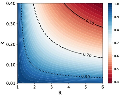
Figure 2 gives an impression of the probability that a single infection will not lead to an outbreak. The result for R<1 are not shown as these values of R<1 cannot lead to an outbreak. For R>1 an outbreak is possible and, after a number of primary cases, must necessarily happen. On average, it will take $1/(1-P)$ primary cases, before an outbreak occurs.

Figure 2. Extinction probability P of an infection chain started by one infected individual, as a function of R and k. The negative binomial distribution (Equation (1(1) $p(n,1)=\frac{\mathrm{\Gamma }(n+k)}{n!\mathrm{\Gamma }(k)}{\left(\frac{k}{k+R}\right)}^k{\left(\frac{R}{k+R}\right)}^n,$(1) )) is not truncated.

6. Truncated negative-binomial distribution

One of the most effective non-pharmaceutical interventions to mitigate the spread of the disease is to limit the number of contacts per person. To illustrate this effect, we consider what would happen if we truncate the negative-binomial distribution at a value $n_t$ where the probability is not yet negligible. However, truncation alone is not enough, because the probability of infecting 1,2,…,$n_t$ persons must still sum to one. There are two ways of normalising the truncated distribution: in one case, we just compute the sum (8) $S_t=\sum _{n=0}^{n_t}p(n,1)$(8) and define the normalised distribution $p^{\prime }(n,1)\equiv p(n,1)/S_t$. But this is not very realistic, because if people do not participate in ‘super-spreader’ events, it does not necessarily mean that they have a much higher chance of infecting people in their ‘bubble’. In what follows, we consider the limiting case that avoiding a super-spreader event does not affect the chances of infecting your closer circle. In that case, $p^{\mathrm{\prime }}(n,1)=p(n,1)$ for $n\ge 1$ and $p^{\mathrm{\prime }}(0,1)=p(0,1)+(1-S_t)$. As before, we can now, compute the probability that a single infected person created an outbreak, and vary $n_t$ from, say 30, all the way down to 1. Note that by decreasing $n_t$, we are decreasing $R_{\mathrm{eff}}$ (Equation (2(2) $R_{\mathrm{eff}}=\sum _{n=1}^{n_t}{p}^{\mathrm{\prime }}(n,1)n,$(2) )). Once $R_{\mathrm{eff}}=1$, no outbreak can occur. For a given value of k, we can use Equation (2(2) $R_{\mathrm{eff}}=\sum _{n=1}^{n_t}{p}^{\mathrm{\prime }}(n,1)n,$(2) ) to determine the value of $n_t$ for which $R_{\mathrm{eff}}$ crosses one: that calculation, although numerical, is trivial and can be done on a spreadsheet [22].

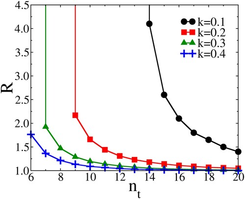
Figure 3 shows a plot of the effect of $n_t$ on the boundary between between outbreak and extinction: Note that by decreasing $n_t$, we are decreasing $R_{\mathrm{eff}}$. As is clear from this figure, a large dispersion (small k) makes a pandemic particularly sensitive to measures that aim to truncate the number of contacts. In real life, the threshold is of course never sharp, but that is not the point here: what we aim to illustrate is that, for the same value of the ‘bare’ $R_0$, it is easier to control a ‘super-spreader’ by social distancing, than a disease that infects people according to a Poisson distribution. The other important point to note is that, for small k, an increase in R above 3–4 barely changes the value of $n_t$ where $R_{\mathrm{eff}}$ dips below one.

Figure 3. As an illustration of the effect of limiting the number of contacts of an individual to $n_t$, the curves in this figure show how the threshold for an outbreak ($R_{\mathrm{eff}}=1$) depends on the bare reproduction number R and the dispersion factor k. For a given value of k, the area to the left of the curve corresponds to the parameter range where no outbreaks occur. In reality, this boundary will not be sharp. Clearly, the effect of limiting the number of contacts is largest for highly over-dispersed distributions (small k). We do not show the result for the Poisson distribution, because in that case truncating $n_t$ has no effect in the range of $n_t$ shown, unless R is very close to one.

7. Number of infected in transient

Consider again the generating function (9) $\tilde{p}(s;1)=\sum _{n}p(n,1)s^n.$(9) The average number of people infected by one person is (10) $⟨n{⟩}_1=\sum _{n}np(n,1)={\left(\frac{\mathrm{\partial }\tilde{p}(s;1)}{\mathrm{\partial }s}\right)}_{s=1},$(10) which is equal to R, as defined before. Similarly, for the number infected by m persons (11) $⟨n{⟩}_m={\left(\frac{\mathrm{\partial }\tilde{p}(s;m)}{\mathrm{\partial }s}\right)}_{s=1}.$(11) We now define a matrix $\mathcal{G}(s)$, with as elements ${\mathcal{G}}_{nm}(s)=G_{nm}{s}^n$. Then the derivative of $\mathcal{G}(s)$ with respect to s is given by (12) ${\mathcal{G}}^{\mathrm{\prime }}=\left(\frac{\mathrm{\partial }\mathcal{G}}{\mathrm{\partial }s}\right),$(12) and for s = 1, ${\mathcal{G}}^{\mathrm{\prime }}$ has as elements (13) ${\mathcal{G}}_{nm}^{\mathrm{\prime }}=np(n,m).$(13) If we consider the derivative (14) ${\left(\frac{\mathrm{\partial }{\mathcal{G}}^k}{\mathrm{\partial }s}\right)}_{s=1}={\mathcal{G}}^{\mathrm{\prime }}{\mathcal{G}}^{k-1}+\mathcal{G}{\mathcal{G}}^{\mathrm{\prime }}{\mathcal{G}}^{k-2}+\cdots +{\mathcal{G}}^{k-1}{\mathcal{G}}^{\mathrm{\prime }},$(14) we can write (15) ${\left(\frac{\mathrm{\partial }{\mathcal{G}}^k}{\mathrm{\partial }s}\right)}_{s=1}={\left(\frac{\mathrm{\partial }(\mathcal{G}+\lambda {\mathcal{G}}^{\mathrm{\prime }}{)}^k}{\mathrm{\partial }\lambda }\right)}_{\lambda =0},$(15) because at $\lambda =0$, the right-hand side only retains all terms linear in ${\mathcal{G}}^{\mathrm{\prime }}$, i.e. the right-hand side of Equation (14(14) ${\left(\frac{\mathrm{\partial }{\mathcal{G}}^k}{\mathrm{\partial }s}\right)}_{s=1}={\mathcal{G}}^{\mathrm{\prime }}{\mathcal{G}}^{k-1}+\mathcal{G}{\mathcal{G}}^{\mathrm{\prime }}{\mathcal{G}}^{k-2}+\cdots +{\mathcal{G}}^{k-1}{\mathcal{G}}^{\mathrm{\prime }},$(14) ). Let us now consider the matrix $\begin{array}{rl}\mathbf{\text{Z}}(\lambda )& \equiv \sum _{k=0}^{\mathrm{\infty }}(\mathcal{G}+\lambda {\mathcal{G}}^{\mathrm{\prime }}{)}^k\\ & =(I-[\mathcal{G}+\lambda {\mathcal{G}}^{\mathrm{\prime }}]{)}^{-1}\\ & =([I-\mathcal{G}][I-[I-\mathcal{G}{]}^{-1}[\lambda {\mathcal{G}}^{\mathrm{\prime }}]{)}^{-1}\\ & =(I-[I-\mathcal{G}{]}^{-1}[\lambda {\mathcal{G}}^{\mathrm{\prime }}]{)}^{-1}(I-\mathcal{G}{)}^{-1}.\end{array}$$\mathbf{\text{Z}}(\lambda )$ is just a generalisation of $\mathbf{\text{Z}}$ defined in Equation (7(7) $\mathbf{\text{Z}}\equiv \sum _{\ell =0}^{\mathrm{\infty }}{G}^n=(I-G{)}^{-1},$(7) ). The total number of infected people in a transient outbreak, $n_{\mathrm{eff}}$, is the 01 element of the derivative (16) $n_{\mathrm{eff}}={\left(\frac{\mathrm{\partial }\mathbf{\text{Z}}(\lambda )}{\mathrm{\partial }\lambda }\right)}_{\lambda =0,s=1}.$(16) We can write (17) $n_{\mathrm{eff}}=[(I-\mathcal{G}{)}^{-1}{\mathcal{G}}^{\mathrm{\prime }}(I-\mathcal{G}{)}^{-1}{]}_{01},$(17) where ${\mathcal{G}}^{\mathrm{\prime }}$ and $\mathcal{G}$ are computed at s = 1. In words, Equation (17(17) $n_{\mathrm{eff}}=[(I-\mathcal{G}{)}^{-1}{\mathcal{G}}^{\mathrm{\prime }}(I-\mathcal{G}{)}^{-1}{]}_{01},$(17) ) expresses the following: the first term describes the probability of propagation from the initial state to the state after $0,1,\dots ,k,\dots$ steps. Then the term $G^{\mathrm{\prime }}$ multiplies that probability with the number of infections generated at that step, and the final term multiplies this number with the probability to reach extinction after another $0,1,\dots ,k^{\mathrm{\prime }},\dots$ steps.

8. Results

Figure 4 shows the dependence of the extinction probability of a transient caused by one person, on the truncation $n_t$ of the negative binomial distribution. Note that by decreasing $n_t$, we are decreasing $R_{\mathrm{eff}}$ (Equation (2(2) $R_{\mathrm{eff}}=\sum _{n=1}^{n_t}{p}^{\mathrm{\prime }}(n,1)n,$(2) )). Once $R_{\mathrm{eff}}=1$, no outbreak can occur. This explains why the curves in Figure 4(a,b) saturate at 1 for a finite value of $n_t$. As mentioned above, that point can be computed trivially by determining the value of $n_t$ for which (18) $\sum _{n=1}^{n_t}n{p}^{\mathrm{\prime }}(n,1;k,R)=1$(18) From Figure 4, it is also clear that for the same value of $R_0$, it is much easier to suppress an outbreak by social-distancing, i.e. by decreasing $n_t$ for low values of k (strong over-dispersion), then it would be for more Poisson-like distributions. This is good news for a disease like COVID19 with an estimated value of k between 0.1 and 0.2. We also note that, not surprisingly, the threshold for an outbreak coincides with the case where one infected person infects, on average, one other. This behaviour is well-known from percolation problems in the physical sciences.

Figure 4. (A) Extinction probability P versus $n_t$ (see text) for $R_0=2$, and $k=0.1$, 0.2, 0.4. (B) Extinction probability P versus $n_t$ for $R_0=5$, and $k=0.1$, 0.2, 0.4. (C) Average number infected versus $n_t$ in a transient outbreak, for $R_0=2$, and k = 0.1, 0.2, 0.4. (D) Average number infected versus $n_t$ in a transient outbreak, for $R_0=5$, and k = 0.1, 0.2, 0.4.

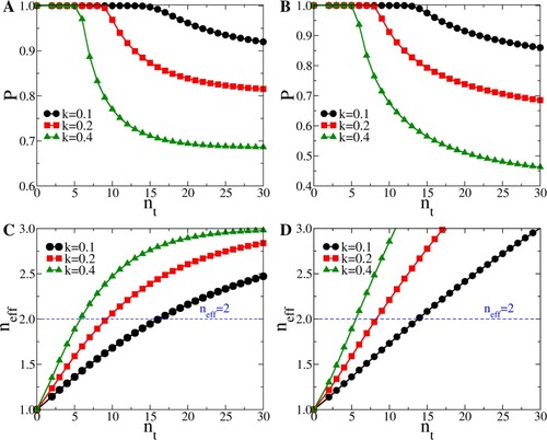
Beyond that threshold, the probability of a full-scale outbreak becomes non-zero, but the actual number of people infected in transients only increases slowly.

9. Discussion

In this paper, we used the negative binomial distribution to describe the number of secondary infections for a single primary case. However, the methods that we use would work just as well for any other plausible distribution that can reproduce over-dispersion, and we do not expect the conclusions to be changed qualitatively.

In the introduction, we noted the difference between our approach and the one used in the standard SEIR models. However, SEIR models can be adapted to account correctly for the probability that m individuals infect n others, using the language of Chemical Master Equations. Such an approach can also be used to arrive at an optimal choice of the ‘point of no return’ ($k_{\max }$) [16]. We did not explore this route, but for practical applications of model studies that include over-dispersion, the continuous-time Chemical Equation Approach is more flexible and potentially more powerful.

Our simple model strongly suggests that over-dispersion, which is related to the tendency of infections to propagate by super-spreader events, makes it easier to control outbreaks by decreasing $n_t$.

It is likely that the probability of infecting n others will be different for people belonging to different categories. In the current model, this entire variation is subsumed in the final $p(n,1)$, which can be viewed as the linear combination of individual distributions. Hence, we do not assume that all individuals/groups have the same spreading pattern. However, we do make a ‘mean-field’ approximation, assuming that there is no correlation between the categories to which infectious and susceptible people belong. Clearly, this is an oversimplification. However, the other ‘strongly correlated’ limit, where spreading is completely within a group with identical spreading behaviour, seems less realistic – but also easy to compute. Of course, the model can be made to account for heterogeneity, but only at the expense of making it more complicated. That is not the aim of the present paper.

Figure 2 suggests that the regional heterogeneity in the observed outbreaks is hard to reconcile with the assumption that $p(n,1)$ is the same everywhere. Rather, we argue that regional differences in $p(n,1)$ are a much more likely explanation for different outbreak probabilities. It would seem plausible to assume that the number of potentially dangerous contacts of people commuting in a big city is larger than the number of contacts of, say, a farmer.

Rather than attributing this difference to $R_0$ or k, one could argue that, effectively, a rural population has a lower $n_t$, except during special events such as Carnival [17]. It is then easy to understand why an outbreak that affects a densely populated area, may not propagate in the countryside. But as is clear from Figure 3, mutations that increase the infectiousness of a virus, even slightly, may foster an outbreak in a region that had thus far been spared.

The steady, low level of infections that were observed in some regions during the first wave of COVID19, is unlikely to be due to repeated extinction of outbreaks in a population with an otherwise homogeneous $p(n,1)$. It is more likely that local outbreaks occurred in venues such as meat factories, that had a larger than average $n_t$, and then petered out when the infections spread into a community where the effective $n_t$ was still below the threshold.

Modelling pandemics is more challenging than molecular simulation.

In the physical sciences, we are in the fortunate situation that the atoms and molecules, which make up the materials that we study, have immutable properties that can be probed in experiments. These experiments range from measuring the equation of state of a bulk sample, to more ‘microscopic’ experiments such as X-ray/neutron-scattering, various forms of microscopy, and much, much more. These data provide essential input for any subsequent modelling.

In a simulation, we usually go through the following ‘checklist’:

1. What are the players (atoms, molecules, proteins, colloids, solvents, substrates…)?

2. What is the best way to describe their interactions? After all, also in the physical sciences, we only know interactions approximately.

3. What is the state of the system, e.g. liquid, crystal, liquid crystal etc.?

4. What properties do we wish to predict? and

5. How should we perform the simulations?

Once we have a good force-field for a given class of molecules, we often assume that if that model worked well for a known system, it will also work for an unknown system – and often that is even true.

Now consider an emerging epidemic. Initially, we know very little about the pathogen, and many of the most important properties of a new pathogen: how it spreads, whom it attacks, how long people are infectious etc., can only be inferred from the outcome of (often Bayesian) simulations [18]. Direct experiments are almost always unethical. How unethical becomes clear if we look at the possibly lethal consequences of one unintended experiment, where the use of outdated spread-sheet software, randomly removed a large subgroup of people who were supposed to be in a UK test-and-trace program [19].

Working with the reported data on different groups in society, the problem arises that the more fine-grained we wish to make our analysis, the fewer data points we have, resulting in poor statistics. Moreover, what we cannot (or do not) measure, we do not detect: a serious problem in the early stages of the COVID19 pandemic. And then, while people are struggling to collect the relevant data, the landscape changes due to interventions, such as banning international travel or imposing lock-downs, imposing mandatory wearing of face masks and, at a later stage, vaccination, and also mutation of the pathogen. All these factors are complicated by varying degrees of (intentional or unintentional) non-compliance.

The factors listed above make it clear that it is extremely difficult to get the information that would be needed to design realistic, fine-grained models. Still, it is worthwhile to consider what such an unachievable model would look like, at least seen from the perspective of someone in the Physical Sciences. The reason for considering such a pipe-dream is not that it will be achievable, but rather that some ways of organising the data would be better suited for data integration than others.

First, we note that numbers such as $R_0$ and k should be outputs of a model that accounts for the biology (what is the minimal infectious dose?), physics (how are the viruses delivered to a susceptible person, and where do they land?) and sociology (who interacts with whom, where and for how long?). Only when we know $R_0$ and k from other sources, can we arrive at the form of $p(n,1)$. But even the negative-binomial form is only an approximation. Hence, we may be able to arrive at more realistic forms for $p(n,1)$.

So, what is primary biological information? First of all the probability per unit time that a susceptible person is infected by someone who is infectious. For a given pathogen, this probability depends on the age, gender, ethnicity etc. of the recipient and on the mode of transmission. This is where the physics comes in: to a first approximation, we can distinguish four major modes of transmission: airborne, direct (or close) contact, touching objects, which are called in the jargon ‘fomites’, but basically they are just objects that can carry the infection, and contact via bodily fluids.

These different modes of transmission become important when we consider the next stage (the sociology): with whom do people interact; how and for how long? Well, that depends: our social network for airborne transmission is totally different from our network for transmission via close, or very close, contact. But, at least some of these networks are knowable and, with the (well-regulated) tracking of mobile phone data (see e.g. [20]) such information is increasingly within reach. Still, different groups (age, ethnicity, gender, socio-economic status,…) have different networks.

Finally, we need to know the distribution of time intervals during which an infected person is infectious – and also whether the disease can be spread by people who seem perfectly healthy, because they are less likely to cut their number of contacts. Actually, the factors listed above are but a small subset of all the parameters that modulate disease transmission [21].

The above discussion makes it clear why modelling pandemics is much harder than modelling molecular systems. However, if we know the dominant mode of transmission, a description based on knowledge of the relevant social interaction network of a given population, combined with knowledge of the primary infectivity of the pathogen should yield numbers such as $R_0$ and the degree of dispersion. Moreover, such models should be able to account for the different spreading patterns of diseases that have a similar mode of propagation, but different infectiousness.

Of course, in practice, we will have to continue using simplified models, but it is clear that good models should be transferable: we should not have to assume that the social network of a person is different for two diseases that spread by the same mechanism. Transferable models should separate the properties of the network, of the individuals who are the nodes in the network, and of the virus. To give an example: if a virus becomes more infectious, we should not have to change the model of the network. But of course, the change of infectiousness may affect different groups differently. Conversely, if a policy changes the connectivity of the network, we should not need to change the properties of its nodes, or of the virus. The concept of transferability is deeply ingrained in the molecular-simulation community, but seems to be less high on the agenda of pandemic-modelling. (In a collection [D.F.] of over 500 recent re/pre-prints on topics related to pandemic modelling, the term ‘transferable never appears, at least not in the context of transferable models. Of course, absence of evidence is not evidence of absence.)

Thus far, we have discussed pandemic modelling as if the need were obvious. It is, however, useful to be precise about what kind of modelling may be useful for what purposes. Clearly, models cannot be used to predict the more distant future, because pandemics are like the weather: predictions tend to be extremely sensitive to small variations in the initial conditions, and become very unreliable after a relatively short time, just like the Lyapunov instability in Molecular Dynamics. However, some important questions can be addressed by modelling:

1. we can use models to gain insight into the mode of propagation of a disease; in other words, we use the models to infer the parameters that we use to describe the spread of the pandemic (e.g. the generation interval, the reproduction number, the period of infectiousness, the degree of over-dispersion …). Such parameter estimates are very important as snapshots. In the case of COVID19, such information was sorely lacking in the early stages of the pandemic.

2. even if models are of limited value for predicting the long-term development of the pandemic, they can be used to compare the expected medium-term impact of mitigation strategies.

In the language of molecular simulations, using models to gain insight would be called ‘computer experiments’, whereas attempting to predict the time evolution of a real pandemic would be called a ‘computer simulation’. The very simple model that we discussed in this paper is the equivalent of a ‘computer experiment’: our aim is not to predict, but (hopefully) to gain insight. One reason why we discussed this specific model is that the generating-functions approach provides an interesting link between pandemics modelling and the description of phenomena such as percolation or branched polymerisation in the physical sciences. As Richard Feynman wrote in volume II (lecture 12) of his Lectures on Physics: ‘The same equations, have the same solutions.’

Acknowledgments

This paper is was written in honour of Mike Klein, who too had to practice social distancing. D.F. expresses his gratitude to Mike who has been a friend and a source of inspiration for close to half a century.

Disclosure statement

No potential conflict of interest was reported by the author(s).

Additional information

Funding

The work was supported by the EU's Horizon 2020 Program through the grant FET-OPEN 766972-NANOPHLOW, by the Chinese National Science Foundation through the grants 11874398 and 12034019, by the Strategic Priority Research Program of the Chinese Academy of Sciences through the grant XDB33000000, and by an international collaboration grant from the K. C. Wong Education Foundation.

References

- K.A. Schneider, G.A. Ngwa, M. Schwehm, L. Eichner and M. Eichner, BMC Infect. Dis. 20 (1), 1–11 (2020). doi:https://doi.org/10.1186/s12879-020-05566-7
- K. Friston, A. Costello and D. Pillay, BMJ Global Health 5 (12), e003978 (2020). doi:https://doi.org/10.1136/bmjgh-2020-003978
- P. Liu, L. McQuarrie, Y. Song and C. Colijn, preprint (2021). medRxiv doi.org/https://doi.org/10.1101/2021.01.12.21249707.
- D.C. Adam, P. Wu, J.Y. Wong, E.H. Lau, T.K. Tsang, S. Cauchemez, G.M. Leung and B.J. Cowling, Nat. Med. 26 (11), 1714–1719 (2020). doi:https://doi.org/10.1038/s41591-020-1092-0
- J.O. Lloyd-Smith, S.J. Schreiber, P.E. Kopp and W.M. Getz, Nature 438 (7066), 355–359 (2005). doi:https://doi.org/10.1038/nature04153
- F. Wong and J.J. Collins, Proc. Natl. Acad. Sci. 117 (47), 29416–29418 (2020). doi:https://doi.org/10.1073/pnas.2018490117
- M. Fukui and C. Furukawa, preprint (2020). MedRxiv doi.org/https://doi.org/10.1101/2020.06.11.20128058.
- A. Grant and P.R. Hunter, preprint (2021). MedRxiv doi.org/https://doi.org/10.1101/2021.01.16.21249946.
- Y.M. Bar-On, R. Sender, A.I. Flamholz, R. Phillips and R. Milo, preprint (2020). arXiv arXiv:2006.01283v3.
- J.C. Taube, P.B. Miller and J.M. Drake, preprint (2021). MedRviv doi.org/https://doi.org/10.1101/2021.01.11.21249622.
- A. Endo, et al. Wellcome Open Res. 5, 67 (2020).
- M.P. Kain, M.L. Childs, A.D. Becker and E.A. Mordecai, Epidemics 34, 100430 (2021). doi:https://doi.org/10.1016/j.epidem.2020.100430
- B.F. Nielsen, L. Simonsen and K. Sneppen, Phys. Rev. Lett. 126 (11), 118301 (2021). doi:https://doi.org/10.1103/PhysRevLett.126.118301
- Q.B. Lu, Y. Zhang, M.J. Liu, H.Y. Zhang, N. Jalali, A.R. Zhang, J.C. Li, H. Zhao, Q.Q. Song, T.S. Zhao, J. Zhao, H.Y. Liu, J. Du, A.Y. Teng, Z.W. Zhou, S.X. Zhou, T.L. Che, T. Wang, T. Yang, X.G. Guan, X.F. Peng, Y.N. Wang, Y.Y. Zhang, S.M. Lv, B.C. Liu, W.Q. Shi, X.A. Zhang, X.G. Duan, W. Liu, Y. Yang and L.Q. Fang, Eurosurveillance 25 (40), 2000250 (2020). doi:https://doi.org/10.2807/1560-7917.ES.2020.25.40.2000250
- J.C. Miller, Infect. Dis. Model. 3, 192–248 (2018). doi:https://doi.org/10.1016/j.idm.2018.08.001
- B. Munsky and M. Khammash, J. Chem. Phys. 124, 044104 (2006). doi:https://doi.org/10.1063/1.2145882
- Q. Chen, M.M. Toorop, M.G. De Boer, F.R. Rosendaal and W.M. Lijfering, BMC Public Health 20 (1), 1–10 (2020). doi:https://doi.org/10.1186/s12889-019-7969-5
- J.D. Peterson and R. Adhikari, (2020) preprint. arXiv:2010.10955.
- T. Fetzer and T. Graeber, preprint (2020). MedRxiv doi.org/https://doi.org/10.1101/2020.12.10.20247080.
- M. Serafino, H.S. Monteiro, S. Luo, S.D. Reis, C. Igual, A.S.L. Neto, M. Travizano, J.S. Andrade and H.A. Makse, preprint (2020). medRxiv doi.org/https://doi.org/10.1101/2020.08.12.20173476.
- L. Pellis, F. Ball, S. Bansal, K. Eames, T. House, V. Isham and P. Trapman, Epidemics 10, 58–62 (2015). doi:https://doi.org/10.1016/j.epidem.2014.07.003
- D. Frenkel, 2021. doi:https://doi.org/10.17863/CAM.70303