Generalised Landau–Teller fitting of the vibrational relaxation rates in atom–diatom collisions: O₂–Ar system as a case study

Abstract

The common trajectory effective mass (CTEM) approach is applied to the calculation of the temperature dependence of the vibrational relaxation rate coefficient k₁₀ in collisions of a diatomic molecule with chemically inert atom on an anisotropic PES. As a case study, we consider the O₂–Ar system for which experimental data across the wide temperature range and ab initio results for the PES are available. It is shown that temperature dependence of the vibrational relaxation rate coefficient k₁₀ is described by the CTEM approach with non-empirical value of the effective Landau–Teller characteristic temperature that indicates the contribution of O₂ rotation in inducing vibrational transition.

GRAPHICAL ABSTRACT

KEYWORDS:

• Vibrational relaxation
• Landau–Teller model
• effect of molecular rotation

1. Introduction

The experimental values of vibration relaxation rate coefficients k₁₀ (T) for $v=1\to v=0$ transitions in diatomic molecules in collision with atom are often represented in the form of the Landau–Teller (LT) temperature dependence or its later generalisations. The original LT paper [1] gives only the exponential factor in the expression of k₁₀ (T). A respective rate coefficient $k_{10}^{\text{LT}}\left(T\right)$ reads (1) $k_{10}^{\text{LT}}\left(T\right)\propto \mathrm{e}\mathrm{x}\mathrm{p}\left(-\frac{3}{2}{\left(\frac{4{\pi }^2{\omega }^2\mu }{{\alpha }_{\text{LT}}^2{k}_{\text{B}}T}\right)}^{1/3}\right)$(1)

This expression refers to the one-dimensional (1D) atom–diatom collision partners of the reduced mass µ moving under the action of a repulsive exponential potential proportional to $\mathrm{e}\mathrm{x}\mathrm{p}(-{\alpha }_{\text{LT}}^{}R)$, where R denotes collision coordinate. In LT model, diatomic molecule is represented by harmonic oscillator with frequency ω. The 3D generalisation of the 1D expression (1) was suggested by Schwartz, Slawsky and Herzfeld (SSH) [2,3] for isotropic exponential interaction with a model coupling between two vibrational states [4,5]. A further refinement of the LT model comes from the first WKB correction to the classical LT exponent [6] which is important in restoring the detailed balance relation between rate coefficients for vibrational deactivation and activation. The respective expression for the rate coefficient known now as a common trajectory (CT) rate coefficient, $k_{10}^{\text{CT}}\left(T\right)$, can be conveniently expressed through two characteristic temperatures – the LT temperature and the vibrational (v) temperature: (2) $T_{\text{LT}}^{}=4{\pi }^2{\omega }^2\mu /{\alpha }_{\text{LT}}^2{k}_{\text{B}},T_{\text{v}}=\hslash \omega /k_{\text{B}}$(2)

In this way (3) $k_{10}^{\text{CT}}\left(T\right)\propto C_{10}^{\text{SSH}}\left(T\right)\mathrm{e}\mathrm{x}\mathrm{p}\left(-\frac{3}{2}{\left(\frac{T_{\text{LT}}^{}}{T}\right)}^{1/3}+\frac{T_{\text{v}}}{2T}\right)$(3) For this model, the temperature dependence of $C_{10}^{\text{SSH}}\left(T\right)$ is also known, $C_{10}^{\text{SSH}}\left(T\right)$ is proportional to $T^{1/3}$. It comes from the interplay of the temperature dependence of the collision number, which is proportional to $T^{1/2}$, and the temperature dependence of the effective energy width in the thermal averaging, $\propto T^{-1/6}$. Expression (3) is widely used for the interpretation of experimental data [7–10].

Within this approach, the question of relation of $T_{\text{LT}}^{}$ to an anisotropic PES remains open. Of course, with a modern computational technique for scattering calculations and available PES that depend on three coordinates (the atom–diatom distance R, the angle θ between the molecular axis and the collision axis and the interatomic distance r in a diatom) the relaxation rate coefficient can be calculated from the state-to-state vibrational–rotational inelastic cross sections. However, the subsequent thermal averaging over initial translational and rotational degrees of freedom is accompanied by tremendous loss of fine dynamical details, such that one is tempted to develop simplified methods that can shed light on some particular features of the relaxation rate coefficients. One of these features is the temperature dependence of the relaxation rate coefficients and its relation to the properties of PES. Here we are encouraged by the remark by Landau and Teller [1] that the main temperature dependence of the relaxation rate coefficients can be deduced from the properties of the atom–diatom interaction for the equilibrium value of r. In other words, the vibrationally inelastic event in this way is related to the vibrationally elastic motion of colliding partners across PES for a fixed value of the vibrational coordinate of the diatom. As a case study, we consider here the relaxation of O₂ in Ar for which there exist a wealth of experimental data from classical works [11–17] discussed at lengths in reviews [8, 9] and supplemented also by recent study [18–20]. Here, we benefit also from information on ab initio PES for this system [21, 22]. We acknowledge also the results of full dynamical calculations of vibrational relaxation of O₂ in Ar [23–26]. In this respect, our study can provide simple (though quite restrictive) insight into the results of complicated numerical calculations of the relaxation rate coefficient.

2. Configuration-dependent transition probability.

In the following, we adopt the common trajectory effective mass (CTEM) approach which represents an approximation to the semiclassical effective mass (SCEM) method used earlier in the interpretation of N₂ relaxation in He [27]. The main difference of the CTEM approach from the standard 3D generalisation of the classical LT model (such as the SSH model) is that here the reduced mass µ is replaced by the configuration-dependent effective mass µ^EM and that the global isotropic repulsive potential is replaced by the local configuration-dependent repulsive potential.

In line with our previous work [27], the semiclassical CTEM rate coefficient is represented as the mean probability-weighted flux $F_{10}^{\text{CTEM}}$ through the dividing surface S* created by revolution of the generatrix $R^{\ast }=R^{\ast }(T,\theta )$ (4) $\begin{array}{l}{k}_{10}^{\text{CTEM}}\left(T\right)=\underset{S^{\ast }}{\int }{F}_{10}^{\text{CTEM}}(T,\theta )d{S}^{\ast },\\ d{S}^{\ast }\left(\theta \right)=2\pi {\left.R^{\ast }\sqrt{{\left(R^{\ast }\right)}^2+{\left(d{R}^{\ast }/d\theta \right)}^2}\right|}_{R^{\ast }=R^{\ast }(T,\theta )}d\theta \end{array}$(4) The mean configuration-dependent flux $F_{10}^{\text{CTEM}}(T,\theta )$ in Equation (4) corresponds to the one-dimensional relative motion of the partners along the driving mode coordinate q through the dividing surface S*. The flux $F_{10}^{\text{CTEM}}(T,\theta )$ is proportional, under near-adiabatic conditions of vibrational transition, to the exponential factor that originates from the product of two exponential factors, one coming from the transition probability at a fixed energy of the driving mode and the other from the Boltzmann distribution.

In what follows, we concentrate on the calculation of the mean exponential factor that determines main features of the temperature dependence of the rate coefficient. According to [27], we introduce the configuration-dependent transition probability which is parameterised by the point $R_{\text{C}}(E,\theta ),\theta$ on the equipotential line $U_{\text{c}}(R,\theta )=E$ or equivalently by E,θ. In the CTEM approximation, the flux is proportional to the exponential factor (5) $F_{10}^{\text{CTEM}}(E,\theta )\propto \mathrm{e}\mathrm{x}\mathrm{p}\left(-2\omega {\tau }^{\text{CTEM}}(E,\theta )\right)$(5) where the exponent contains the characteristic CTEM collision time ${\tau }^{\text{CTEM}}(E,\theta )$ (6) ${\tau }^{\text{CTEM}}(E,\theta )=\frac{1}{2}\underset{q_t(E,\theta )}{\overset{q_s}{\int }}\frac{\sqrt{2{\mu }^{\text{EM}}(E,\theta )}dq}{\sqrt{U^{\text{CT}}\left(q,\theta \right)-E}}$(6)

The quantity ${\tau }^{\text{CTEM}}(E,\theta )$ refers to the driving mode coordinate q that starts at the point $R_{\text{C}}(E,\theta ),\theta$ (turning point q_t) and runs in the classically forbidden region of the common potential $U^{\text{CT}}\left(q;\theta \right)$ along $\text{grad}U(R,\theta )$ until the integral over q can be considered as converged (the upper limit q_s). The driving mode is a specific combination of the coordinate displacements ΔR and Δθ that describes the motion in a small region centred at $R_{\text{C}}(E,\theta ),\theta$. In this way, the two-dimensional potential $U(R+\mathrm{\Delta }R,\theta +\mathrm{\Delta }\theta )$ is then replaced by a one-dimensional potential $U^{\text{CT}}(q;\theta )$ along $\text{grad}U(R,\theta )$. As in our earlier work [27], we approximate $U^{\text{CT}}\left(q;\theta \right)$ by an exponential function of q with the characteristic slope parameter α^CT defined by the gradient of $U(R,\theta )$ as (7) ${\alpha }^{\text{CT}}(E,\theta )={|\text{grad}U(R,\theta )|}_{R_{\text{C}}(E,\theta ),\theta }/E$(7) Then, the expression in Equation (6) becomes (8) ${\tau }^{\text{CTEM}}(E,\theta )=\pi \sqrt{{\mu }^{\text{EM}}(E,\theta )}/{\alpha }^{\text{CT}}(E,\theta )\sqrt{2E}$(8)

The effective mass µ^EM that enters into Equations (6) and (8) takes into accounts that motion along q near q_t is a superposition of the atom–diatom radial motion and the rotational motion of the diatom with respect to the collision axis. Explicitly, the expression for µ^EM (E,θ) reads [27] (9) $\frac{{\mu }^{\text{EM}}(E,\theta )}{\mu }={\left(1+\frac{\mu }{M{r}_e^2}{\left(\frac{\mathrm{\partial }{R}_{\text{C}}}{\mathrm{\partial }\theta }\right)}^2\right)}^{-1}$(9) where M and r_e are the reduced mass of the diatom and its equilibrium interatomic distance, respectively. This expression is valid when the anisotropy of PES, characterised by the ratio $|\mathrm{\partial }{R}_{\text{C}}/R_{\text{C}}\mathrm{\partial }\theta |$, is not too large, i.e. $|\mathrm{\partial }{R}_{\text{C}}/R_{\text{C}}\mathrm{\partial }\theta |<<1$. We also note that foregoing condition permits one to regard the dividing surface S* in Equation (4) as a sphere. Nonetheless, the second term in the parentheses in r.h.s. of Equation (9) can be noticeable provided the ratio $\mu R_{\text{C}}^2/M{r}_e^2$ is large enough.

The thermal averaging of the flux that transforms $F_{10}^{\text{CTEM}}(E,\theta )$ into $F_{10}^{\text{CTEM}}(T,\theta )$ is accomplished by the steepest descent (SD) approximation, yielding (10) ${\overline{P}}_{10}^{\text{CTEM}}(T,\theta )\propto \mathrm{e}\mathrm{x}\mathrm{p}\left(-2\omega {\tau }^{\text{CTEM}}(E^{\ast },\theta )-E^{\ast }/k_{\text{B}}T\right)$(10) where the optimal energy $E^{\ast }=E^{\ast }(T,\theta )$ is found from the SD condition (11) $2\omega d{\tau }^{\text{CTEM}}(E,\theta )/dE{|}_{E=E^{\ast }}+1/k_{\text{B}}T=0$(11)

The solution of Equation (11) with account taken for Equations (7)–(9) yields the function $E^{\ast }=E^{\ast }(T,\theta )$ and thus the exponent in Equation (10) for a fixed θ. A minimum of $E^{\ast }(T,\theta )$ with respect to θ determines the optimal configuration R*,θ*. We also note that the equation $E^{\ast }(T,\theta )=U(R^{\ast },\theta )$ defines the curve $R^{\ast }=R^{\ast }(T,\theta )$ which serves as a generatrix of the ‘dividing surface’ in Equation (4) (vide supra).

For an isotropic exponential interaction, with $U(R,\theta )=U\left(R\right)\propto \mathrm{e}\mathrm{x}\mathrm{p}(-\overline{\alpha }R)$ and E being the radial collision energy, the time ${\tau }^{\text{CTEM}}$ coincides with the characteristic time for a collinear collision discussed by Landau and Teller [1]: (12) ${\tau }^{\text{LT}}=\pi \sqrt{\mu }/\overline{\alpha }\sqrt{2E}$(12) where the energy dependence of ${\tau }^{\text{LT}}$ appears explicitly. Then equation in Equation (11) can be solved explicitly to give (13) $\begin{array}{rl}{E}_{\text{LT}}^{\ast }& =k_{\text{B}}{T}_{\text{LT}}^{\ast }=\frac{k_{\text{B}}T}{2}{\left(\frac{T_{\text{LT}}}{T}\right)}^{1/3}\end{array}$(13) with T_LT defined by Equation (2).

In general case, it is convenient to represent the exponential in Equation (10) as (14) ${\overline{P}}_{10}^{\text{CTEM}}(T,\theta )\propto \mathrm{e}\mathrm{x}\mathrm{p}\left(-\frac{3}{2}{\left(\frac{T_{\text{LT}}}{T}\mathrm{\Theta }(T,\theta )\right)}^{1/3}\right)$(14) Here T_LT is introduced as a reference quantity from Equation (2), and $\mathrm{\Theta }(T,\theta )$ is a correction function. With a reasonably defined steepness parameter $\overline{\alpha }$, the function $\mathrm{\Theta }(T,\theta )$ is expected to be not too different from unity across the whole range of θ $(0\le \theta \le \pi )$ and the temperature range of interest.

If the preexponential factor in the expression in Equation (12) is known, i.e. the probability ${\overline{P}}_{10}^{\text{CTEM}}(T,\theta )$ is represented as (15) $\begin{array}{rl}& {\overline{P}}_{10}^{\text{CTEM}}(T,\theta )\\ & =A_{10}^{\text{CTEM}}(T,\theta )\mathrm{e}\mathrm{x}\mathrm{p}\left(-\frac{3}{2}{\left(\frac{T_{\text{LT}}}{T}\mathrm{\Theta }(T,\theta )\right)}^{1/3}+\frac{T_v}{2T}\right)\end{array}$(15) it can be used in Equation (4) for calculation of $k_{10}^{\text{CTEM}}\left(T\right)$. With the exponential accuracy, $k_{10}^{\text{CTEM}}\left(T\right)$ from Equation (15) can be estimated as (16) $k_{10}^{\text{CTEM}}\left(T\right)\propto \mathrm{e}\mathrm{x}\mathrm{p}\left(-\frac{3}{2}{\left(\frac{T_{\text{LT}}^{\ast }}{T}\right)}^{1/3}+\frac{T_v}{2T}\right),$(16) where (17) $T_{\text{LT}}^{\ast }=T_{\text{LT}}{\mathrm{\Theta }}^{\ast }\left(T\right)$(17) with $\mathrm{\Theta }(T,\theta )$ being the minimal value of $\mathrm{\Theta }(T,\theta )$ with respect to θ which is attained at θ = θ*: (18) ${\mathrm{\Theta }}^{\ast }\left(T\right)=\underset{\theta }{min}\left\{\mathrm{\Theta }(T,\theta )\right\}=\mathrm{\Theta }(T,\theta ){|}_{\theta ={\theta }^{\ast }}$(18)

If, in addition, ${\mathrm{\Theta }}^{\ast }\left(T\right)$, in the temperature range of interest, weakly depends on T, and one replaces ${\mathrm{\Theta }}^{\ast }\left(T\right)$ by a certain constant ${\overline{\mathrm{\Theta }}}^{\ast }={\mathrm{\Theta }}^{\ast }\left(\overline{T}\right)$ at the reference temperature $\overline{T}$, expression in Equation (16) becomes (19) $k_{10}^{\text{CTEM}}\left(T\right)\approx {\overline{k}}_{10}^{\text{LT}}\left(T\right)\propto \mathrm{e}\mathrm{x}\mathrm{p}\left(-\frac{3}{2}{\left(\frac{{\overline{T}}_{\text{LT}}^{\ast }}{T}\right)}^{1/3}+\frac{T_v}{2T}\right)$(19) with ${\overline{T}}_{\text{LT}}^{\ast }=T_{\text{LT}}{\overline{\mathrm{\Theta }}}^{\ast }$.

In a more accurate treatment, one can assume the standard θ dependence of $A_{10}^{\text{CTEM}}(T,\theta )$ which follows from the SSH model, $A_{10}^{\text{CTEM}}(T,\theta )\propto {\cos }^2\theta$. Then, Equation (3) transformed into the form that contains standard LT exponential, assumes the form (20) $k_{10}^{\text{CTEM}}\left(T\right)=B(T,\overline{T})C_{10}^{\text{LT}}\left(T\right)\mathrm{e}\mathrm{x}\mathrm{p}\left(-\frac{3}{2}{\left(\frac{{\overline{T}}_{\text{LT}}^{\ast }}{T}\right)}^{1/3}+\frac{T_v}{2T}\right)$(20) where the preexponential $B(T,\overline{T})$ includes contributions from θ and T dependence of the CTEM exponents. In this way, the factor $B(T,\overline{T})$ is written as (21) $\begin{array}{rl}B(T,\overline{T})& =b_1\left(T\right)b_2(T,\overline{T}),\\ b_1\left(T\right)& =\underset{0}{\overset{\pi }{\int }}\left(3/2\right){\cos }^2\theta \\ & \times \mathrm{e}\mathrm{x}\mathrm{p}\left[-\frac{3}{2}{\left(\frac{T_{\text{LT}}\left(\mathrm{\Theta }\right(T,\theta )-{\mathrm{\Theta }}^{\ast }(T\left)\right)}{T}\right)}^{1/3}\right]\sin \theta d\theta ,\\ b_2(T,\overline{T})& =\mathrm{e}\mathrm{x}\mathrm{p}\left\{-\frac{3}{2}{\left(\frac{T_{\text{LT}}\left[{\mathrm{\Theta }}^{\ast }\left(T\right)-{\overline{\mathrm{\Theta }}}^{\ast }\right]}{T}\right)}^{1/3}\right\}\end{array}$(21)

The factor b₁(T) roughly corresponds to the range of θ, Δθ that contributes to the vibrational transition, $\mathrm{\Delta }\theta /\pi <1$. It is expected to have a weak positive temperature dependence due to the broadening of the effective integration range over θ. The factor $b_2(T,\overline{T})$ compensates the inconsistency in replacing the temperature-dependent quantity $T_{\text{LT}}^{\ast }$ in Equation (16) by the temperature-independent quantity ${\overline{T}}_{\text{LT}}^{\ast }$ in Equation (19). If ${\mathrm{\Theta }}^{\ast }\left(T\right)$ has a positive temperature dependence (as is the case for O₂–Ar relaxation, see Section 3), the factor $b_2(T,\overline{T})$ has a negative temperature dependence and passes through unity at $T=\overline{T}$. The expression in Equation (20) formally looks like a corrected (correction factor B) SSH expression. However, now the LT temperature ${\overline{T}}_{\text{LT}}^{\ast }$ is not a fitting parameter, but rather a quantity that directly related to the parameters of PES, reduced mass of the partners and the reduced mass of the diatom.

3. Application to O₂–Ar system

In this section, we illustrate the general features described in Section 2 by the vibrational relaxation of O₂ in Ar. For this purpose, we use ab initio PES from [22] and experimental data from recent work [18–20]. The contour map of the potential for O₂–Ar system with equilibrium distance between O–O atoms is presented in Figure 1.

Figure 1. The contour map of the potential for O₂–Ar system (red full lines). Equipotential contours $R_{\text{C}}(E,\theta )$ are shown for values of $T_E=E/k_{\text{B}}$ equal to 500 K (a), 1200 K (b), 2500 K (c), 5000 K (d), 10,000 K (e), 20,000 K (f) and 40,000 K (g). Dashed green line corresponds to the optimal energy $E^{\ast }(T,\theta )$ for $v=1\to v=0$ transition at $T=3000\text{K}$. Optimal configuration at ${\theta }^{\ast }=0.35\pi$ is marked by a small circle. The driving mode corresponds to the coordinate q, and its full part indicates the range ${1/\alpha }^{\text{CT}}(E^{\ast },{\theta }^{\ast }){|}_{T=3000\text{K}}$.

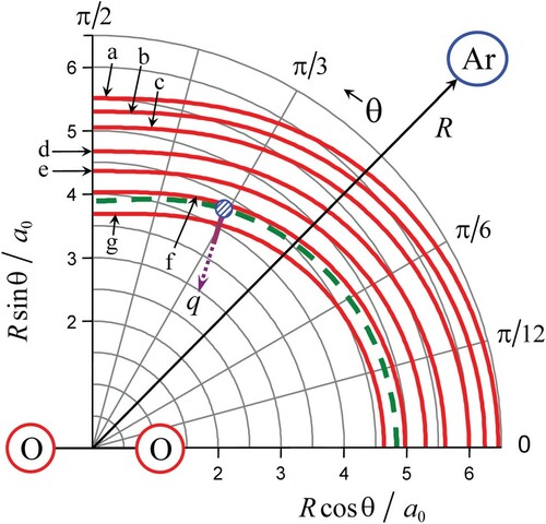
Shown here are several equipotential contours (red full lines) with green dashed curve for $E=E^{\ast }(T,\theta ){|}_{T=3000\text{K}}$. superimposed on them. The full portion of the driving mode coordinate q qualitatively indicates the range $1/{\alpha }^{\text{CT}}(E^{\ast },\theta ){|}_{T=3000\text{K}}$.

The main features of the vibrational relaxation rate coefficient $k_{10}^{\text{CTEM}}\left(T\right)$ for O₂ at collision with Ar are summarised below in items (i)–(v) related to results of Section 2.

(i). The calculated quantities ${\mu }^{\text{EM}}(E,\theta )/\mu$ (left part) and ${\alpha }^{\text{CT}}(E,\theta )$ (right part) from Equations (7) and (9) are shown in Figure 2 as plots vs. θ for different values of $E$. Since plots are symmetrical with respect to $\theta =\pi /2$, only halves of them are shown.

Figure 2. Plots of ${\alpha }^{\text{CT}}(E,\theta )$ and ${\mu }^{\text{EM}}(E,\theta )$ vs. θ for different values of E. The range of E shown roughly corresponds to that of the optimal energy E* (see Figures 3 and 4). All curves ${\mu }^{\text{EM}}(E,\theta )$ collapse into a single one.

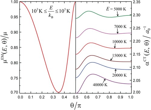
A noticeable increase of ${\alpha }^{\text{CT}}(E,\theta )$ with decreasing E reflects the effect of weak attraction at large interpartner distances. A slight variation of ${\alpha }^{\text{CT}}(E,\theta )$ with θ (for a fixed E) is presumably due to two maxima of the electron density of O₂ that come from the outer MO orbital of O₂. The angular dependence of the ratio ${\mu }^{\text{EM}}/\mu$ comes from the interplay of the large value of the mean frequencies ratio for the rotation of the complex to that of the molecule, $\sqrt{\mu }{R}^{\ast }/\sqrt{M}{r}_e$, and the small interaction anisotropy characterised by the parameter $|d{R}^{\ast }/R^{\ast }d\theta |$. A small value of this parameter, $|d{R}^{\ast }/R^{\ast }d\theta |<<1$, serves as a condition of applicability of the EM expression in the form given by Equation (9). The dependence of ${\mu }^{\text{EM}}(E,\theta )$ on E is so weak that it remains indiscernible.

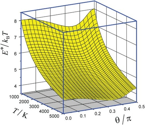
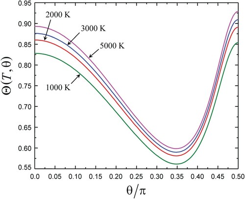
(ii). The optimal energy $E^{\ast }=E^{\ast }(T,\theta )$ which determines the CTEM exponent in Equation (10) was found from numerical solutions of Equation (11) in conjunction with definitions of ${\alpha }^{\text{CT}}(E,\theta )$ and ${\mu }^{\text{EM}}(E,\theta )$ by Equations (7) and (9). The surface plot of $E^{\ast }(T,\theta )$ vs. T and θ is shown in Figure 3 in which the optimal configuration is indicated (see below, item iv). Sections of this surface plot for several values of θ are shown in Figure 4.

Figure 3. 2D plot of the scaled optimal energy for the relaxing O₂–Ar system vs. T and θ. Red full line corresponds to the optimal configurations and a small circle to that in Figure 1.

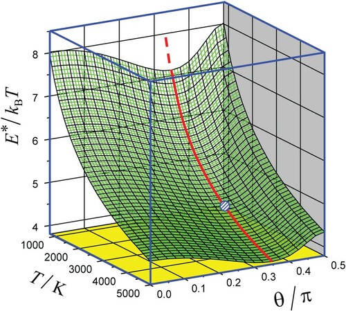
Figure 4. Plots of the optimal energies E* vs. T for different angles θ.

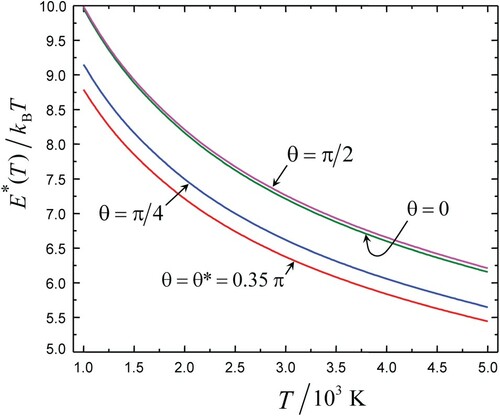
Note that the relation $E^{\ast }>>k_{\text{B}}T$ which is fulfilled for all graphs is the condition of applicability of the SD approximation for the calculation of the CTEM exponent. The drop of the ratio $E^{\ast }(T,\theta )/k_{\text{B}}$ with increasing T indicates at virtual breakdown of the SD approximation at very high temperatures.

(iii). The CTEM correction function $\mathrm{\Theta }(T,\theta )$ was calculated from the CTEM exponent in Equation (10) by factoring out a reference LT temperature with $\overline{\alpha }=1.9a_0^{-1}$ as taken from the highly repulsive portion of PES reported in [22]. Plots of $\mathrm{\Theta }(T,\theta )$ vs. θ for different temperatures are shown in Figure 5 within the range $0\le \theta \le \pi /2$.

Figure 5. Plots of the correction CTEM function $\mathrm{\Theta }(T,\theta )$ vs. θ for different temperatures.

For a fixed T, the global θ dependence of $\mathrm{\Theta }(T,\theta )$ reflects that of ${\mu }^{\text{EM}}(E,\theta )/\mu$ with negligible dependence of ${\mu }^{\text{EM}}(E,\theta )$ on E. For a fixed θ, the dependence of $\mathrm{\Theta }(T,\theta )$ on T reflects increase of ${\alpha }^{\text{CT}}(E^{\ast },\theta )$ with decreasing E*.

(iv). The optimal configuration of the collision complex O₂–Ar for the $v=1\to v=0$ transition at $T=3000\text{K}$ corresponds to the coordinates $R=R^{\ast }(T,{\theta }^{\ast })=4.27a_0,\theta ={\theta }^{\ast }=0.35\pi$, it is marked by a circle in Figures 1 and 3.

(v). Within the interval where the high precision experimental data are available, the temperature dependence of $B(T,\overline{T})$ is quite weak such that the overall temperature dependence of the CTEM rate coefficient is close to that of SSH rate coefficient provided that the LT temperature, T_LT, of the latter is identified with ${\overline{T}}_{\text{LT}}^{\ast }$.

The comparison of CTEM rate coefficient from Equations (20)–(21) (full line) with experimental data is presented in Figure 6. Previous experimental results taken from Refs. [13,16,17] (open symbols) are shown only for temperature range where recently measured high precision data ([18–20], red filled symbols) are not available.

Figure 6. Comparison of CTEM rate coefficient from Equations (20), (21) (full line) with experiment. The CTEM rate coefficient was fitted (by a scaling prefactor) to experimental data at T = 4000 K. Experimental data measured recently with high precision are shown by filled red symbols: squares [18], triangles [19] and circles [20]. Earlier experimental results are presented by open symbols: green triangles [13], blue squares [16], and magenta rhombs [17]. The dotted line corresponds to the case when the rotation of O₂ is ignored (µ^EM = µ).

For this case, theoretical value of ${\overline{T}}_{\text{LT}}^{\ast }$, calculated for $\overline{T}=2000\text{K}$, is $3.3\cdot {10}^6\text{K}$. This would correspond to expression in Equation (2) where ratio ${\mu }^{\text{EM}}/\mu =0.7$ (i.e. µ is replaced by $\tilde{\mu }=0.7\mu =12.5\text{a}\text{.m}\text{.u}\text{.}$) and α by $\tilde{\alpha }=2.10a_0^{-1}$. Also shown is LT plot for the same value of α and for ${\mu }^{\text{EM}}/\mu =1.0$, what is equivalent to ${\overline{T}}_{\text{LT}}^{\ast }=4.7\cdot {10}^6\text{K}$ (dotted line). In this case common trajectory model is used, but rotation of molecule in vibrational relaxation event is neglected.

4. Conclusion

The common trajectory effective mass (CTEM) approach describes the collision-induced 1–0 vibrational transition in a diatom as induced by the classical translational–rotational motion of an atom–diatom system across the PES for the atom–diatom interaction at the equilibrium value of the vibrational coordinate of the diatom. The CTEM rate coefficient is calculated up to a temperature-independent scaling coefficient which incorporates the coupling of diatom vibration to the translation and rotation of the collision system. The application of the theoretical results to the vibrational relaxation of O₂ in Ar allows one to rationalise the experimental temperature dependence of the rate coefficient in terms of the effective Landau–Teller temperature calculated from ab initio PES. The latter indicates at the noticeable participation of the rotation of O₂ in the inducing vibrational transition which shows in the substantial decrease of the effective mass in the optimal configuration of the collision complex. This is at variance with our earlier findings for N₂–He system where the rotational contribution was found to be small [27]. The explanation goes back to different values of the ratio $\mu /M$ which is larger than unity for O₂–Ar and smaller than unity for N₂–He.

In summary, we regard the common trajectory, CT (motion along a classical trajectory running across a common potential that simulates two vibrationally adiabatic potentials originating from two vibrational states of a diatom) effective mass, EM (simulation of a two-dimensional trajectory in the $R,\theta$ space by an one-dimensional trajectory in the motion along the driving mode coordinate) approach (CTEM) as a reasonable approximation in the problem of VRT energy transfer under conditions of high temperatures and not very strong anisotropy (see comments in Section 3) for interpretation of experimental temperature dependence of the relaxation rate coefficient $k_{10}\left(T\right)$ in terms of the properties of the PES for an atom and a non–vibrating diatom.

Acknowledgements

This paper acknowledges many stimulating discussions with Professor J. Troe and his continuing interest in our work.

Disclosure statement

No potential conflict of interest was reported by the author(s).

References

- L. Landau and E. Teller, Phys. Z. Sowjetunion. 10, 34 (1936).
- R.N. Schwartz, Z. Slawsky and K.F. Herzfeld, J. Chem. Phys. 20, 1591 (1952). doi:https://doi.org/10.1063/1.1700221
- R.N. Schwartz and K.F. Herzfeld, J. Chem. Phys. 22, 767 (1954). doi:https://doi.org/10.1063/1.1740190
- T.L. Cottrell and J.C. McCoubrey, Molecular Energy Transfer in Gases (Butterworths, London, 1961).
- E.E. Nikitin, Theory of Elementary Atomic and Molecular Processes in Gases (Clarendon Press, Oxford, 1974).
- E.E. Nikitin and J. Troe, Phys. Chem. Chem. Phys. 8, 2012 (2006). doi:https://doi.org/10.1039/B517843F
- B.F. Gordiets, A.I. Osipov and L.A. Shelepin, Kinetic Processes in Gases and Molecular Lasers (Gordon and Breach, New York London Paris, 1988).
- E.E. Nikitin, A.I. Osipov and S.Y. Umansky, in Reviews of Plasma Chemistry, edited by B.M. Smirnov (Consultants Bureau, New York London, 1994).
- M. Capitelli, C.M. Ferreira, B.F. Gordiets and A.I. Osipov, Plasma Kinetics in Atmospheric Gases (Springer, Berlin Heidelberg, 2000).
- R. Brun, High Temperature Phenomena in Shock Waves (Springer, Berlin Heidelberg, 2012).
- M. Camac, J. Chem. Phys. 34, 448 (1961). doi:https://doi.org/10.1063/1.4757208
- K.I. Wray, J.Chem. Phys. 37, 1254 (1962). doi:https://doi.org/10.1063/1.1733273
- D.R. White and R.C. Millikan, J. Chem. Phys. 39, 1807 (1963). doi:https://doi.org/10.1063/1.1734533
- R.C. Millikan and D.R. White, J. Chem. Phys. 39, 3209 (1963). doi:https://doi.org/10.1063/1.1734182
- N.A. Generalov and S.A. Losev, J. Quan. Spectrosc. Radiat. Transfer. 6, 101–125 (1966). doi:https://doi.org/10.1016/0022-4073(66)90066-5
- C. Chiang and G.B. Skinner, J. Quan. Spectrosc. Radiat. Transfer. 24, 525–528 (1980). doi:https://doi.org/10.1016/0022-4073(80)90021-7
- V.S. Rao and G.B. Skinner, J. Chem. Phys. 81, 775–779 (1984). doi:https://doi.org/10.1063/1.447710
- J.W. Streicher, A. Krish, R.K. Hanson, K.M. Hanquist, R.S. Chaudhry and I.D. Boyd, Phys. Fluids. 32, 076103 (2020). doi:https://doi.org/10.1063/5.0012426
- J. W. Streicher, A. Krish, S. Wang, D. F. Davidson, and R. K. Hanson, AIAA Report 2019–0795, AIAA Science and Technology Forum and Exposition – Non–Equilibrium Flows I, San Diego, CA (2019).
- K.G. Owen, D.F. Davidson and R.K. Hanson, J. Thermophys. Heat Transfer. 30, 791–798 (2016). doi:https://doi.org/10.2514/1.T4505
- F.A. Gianturco and A. Storozhev, J. Chem. Phys. 101, 9624 (1994). doi:https://doi.org/10.1063/1.467927
- S.M. Cybulski, R.A. Kendal, G. Chalasinski, M.W. Severson and M. Szczesniak, J. Chem. Phys. 106, 7731 (1997). doi:https://doi.org/10.1063/1.473798
- I. S. Ulusoy, D. A. Andrienko, I. D. Boyd, and R. Hernandez, AIAA Report 2017–0661, AIAA Science and Technology Forum and Exposition – Aerothermodynamics II, 55th AIAA Aerospace Sciences Meeting, Grapevine, Texas (2017). https://doi.org/https://doi.org/10.2514/6.2017-0661
- I.S. Ulusoy, D.A. Andrienko, I.D. Boyd and R. Hernandez, J. Chem. Phys. 144, 234311 (2016). J. Chem. Phys. 145, 239902 (2016) [Erratum]. doi:https://doi.org/10.1063/1.4954041
- J.G. Kim and I.D. Boyd, Chem. Phys. 446, 76–85 (2015). doi:https://doi.org/10.1016/j.chemphys.2014.11.009
- K. M. Hanquist, R. S. Chaudhry, I. D. Boyd, J. W. Streicher, A. Krish, and R. K. Hanson, AIAA Report 2020–3275, AIAA Aviation Forum – Hypersonics, Virtual Event (2020). https://doi.org/https://doi.org/10.2514/6.2020-3275
- E.I. Dashevskaya, I. Litvin, E.E. Nikitin and J. Troe, J. Chem. Phys. 125, 154315 (2006). doi:https://doi.org/10.1063/1.2357951