
 ?Mathematical formulae have been encoded as MathML and are displayed in this HTML version using MathJax in order to improve their display. Uncheck the box to turn MathJax off. This feature requires Javascript. Click on a formula to zoom.
Abstract
Parity and nuclear spin symmetry are approximate symmetries, which for many primary processes in molecular spectroscopy and kinetics lead to almost exact constants of the motion. The symmetric isotopomer dichlorodisulfane (disulfur dichloride) is chiral with two enantiomers, each of which has also two nuclear spin isomers (ortho and para isomers). Electroweak quantum chemistry predicts a small ‘parity violating’ energy difference
between the ground states of the enantiomers (M being more stable than P by about
). Furthermore recent microwave spectroscopy has indicated ‘forbidden’ transitions between ortho and para isomers. These phenomena allow for a comparative study of the time-dependent quantum dynamics of parity and nuclear spin symmetry violation in a chiral molecule for the first time. We report quantum dynamical calculations of coherent radiative excitation of the complex manifold of polyads with hyperfine structure in ClSSCl. We demonstrate almost complete (near 100%) transfer of population from an almost pure para-ground state to an almost pure excited ortho state. Short-pulse excitation from the para-ground state to an excited time-dependent para chromophore state shows intramolecular interconversion between para and ortho nuclear spin isomers under isolation after the pulse on a time scale of a few nanoseconds to a few microsecond depending on the excited polyad. We also demonstrate the preparation of exotic ‘chameleon states’, which are superpositions of energy eigenstates corresponding to ortho- and para- nuclear spin symmetry isomers at the same time. The results are discussed in relation to the strong separation of time scales between the primary processes of nuclear spin symmetry isomerisation (nanoseconds to microseconds) and parity change (seconds) and in relation to possible experiments to measure
in this molecule. We also compare with the rate processes of nuclear spin symmetry isomerisation induced by thermal black body radiation, depending on temperature, occurring on time scales from less than seconds to more than 100 years.
GRAPHICAL ABSTRACT
1. Introduction
Jürgen Troe is known as a pioneer of short-time kinetics, who studied molecular primary processes in the picosecond time scale already prior to the availability of picosecond lasers, for example in his fundamental work on the dissociation of NO [Citation1–3]. Over the following decades, his research was extended far into the subpicosecond and femtosecond range, using laser techniques, but by no means restricted to these, in fact covering an exceptionally large range of methods from shock-waves to lasers, ranging from the lowest to the highest pressures in the gas phase and condensed phases, developing advanced and ingenious experimental approaches as well as theoretical methods. Some of this can be found summarised in the short survey given in [Citation4], by no means complete and continuing until today. While there existed many efforts on femtosecond laser chemistry following developments after 1980 [Citation5], Jürgen Troe has been exceptional in combining his experiments with deep theoretical insight as well as an understanding of practical applicability to problems of direct relevance to combustion, atmospheric chemistry, astrochemistry and photochemistry [Citation6,Citation7].
In recent years, the frontier of short-time kinetics and dynamics has moved into the sub-femtosecond and attosecond time ranges by generating laser pulses of ever shorter duration (see [Citation8–15] and references cited therein). We have pointed out, however, that an altogether completely different approach avoiding ultrashort laser pulses but rather using high frequency resolution at long times combined with advanced analysis can cover primary processes from very long times to the shortest, with femtosecond and possibly subfemtosecond characteristics [Citation16–19] and even extending into the yoctosecond domain, in principle ([Citation20] and references cited therein). Using this approach along very different lines, we have discussed that by slowing down one can explore a completely different, new frontier relating primary processes to fundamental symmetries of physics and chemistry. For instance, experiments on the kinetics of parity change in isolated chiral molecules can open a window to possibly new physics [Citation21,Citation22] and is expected to allow for the determination of the extremely small parity violating energy difference between the ground states of chiral molecules [Citation23]. While theoretical predictions for this quantity in the feV and sub-feV range exist ([Citation24] and references cited therein) no successful experiment has so far been carried out although a current experimental setup has demonstrated the accessibility of the range towards
in a proof of principle experiment on the achiral molecule NH
[Citation25]. Current efforts concentrate on the exploration of suitable chiral molecules for such experiments. Among possible candidates are the disulfanes (or also disulfides/disulphides).
The disulfide compounds X–S–S–Y contain a non-planar, intrinsically chiral structural element, and are of importance in a variety of contexts ranging from biological chemistry [Citation26] to the theory of molecular structure [Citation27] and astrophysics [Citation28–31]. A more recent focus has been the possibility of experiments on parity violation in such chiral molecules. While the simplest ‘parent’ molecule disulfane HSSH has a relatively large tunneling splitting of about in the ground state, which largely suppresses the effects from parity violating potentials on the order of
, other disulfides with heavier substituents show tunneling splittings smaller than parity violating energies and are thus dominated by parity violation [Citation24,Citation32–35]. Notably for the prototypical C
-symmetrical chiral molecule Cl–S–S–Cl (Figure ) we have shown some time ago that with a barrier of more than
for the interconversion of the enantiomers one can estimate a tunneling splitting much less than
for the hypothetical, symmetrical, parity conserving potential. The theoretically predicted parity violating energy difference
of
between the P- and the more stable M-enantiomer thus exceeds the tunneling splitting by several ten orders of magnitude [Citation36]. Therefore the quantum structure and dynamics of this molecule are completely dominated by parity violation, similar to, say, the prototypical tetrahedral organic molecule CHFClBr with a comparable predicted parity violating energy difference
of about
[Citation37,Citation38]. Thus ClSSCl exists at low energies in the form of two energetically slightly different isomers with ground state wavefunctions localised around the equilibrium structures of the enantiomers and ground state energies predicted to be separated by
(
). While this energy difference is too small to be directly measurable in a thermochemical or even high-resolution spectroscopic experiment, it can be obtained with the time-dependent technique proposed in [Citation23], if a suitable excited achiral electronic state can be identified for applying the scheme of Ref. [Citation23,Citation39]. Our experimental setup has shown sufficient sensitivity to measure energies on the order of
[Citation25]. In a time-dependent spectrum, one would observe the small change of parity by the violation of that symmetry, on a ms time scale (with a predicted period of motion of about
for ClSSCl [Citation36]).
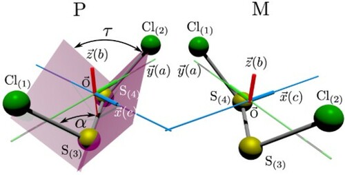
Figure 1. Perspective drawing of the equilibrium structure and axes definitions for the P and M enantiomers of (as calculated in [Citation36]). The axis in the I
representation for the A-reduced Watson Hamiltonian used in the analysis of the spectra are
,
,
(with a,b,c being the principal inertial axes). The C
symmetry axis coincides with the b-axis.
![Figure 1. Perspective drawing of the equilibrium structure and axes definitions for the P and M enantiomers of 35Cl−32S−32S−35Cl (as calculated in [Citation36]). The axis in the Ir representation for the A-reduced Watson Hamiltonian used in the analysis of the spectra are x′=b, y′=c, z′=a (with a,b,c being the principal inertial axes). The C2 symmetry axis coincides with the b-axis.](/cms/asset/6c9a26a3-777e-48cd-9ac5-95ff4de0e376/tmph_a_1959073_f0001_oc.jpg)
Recently a further interesting phenomenon has been observed for this molecule. As ClSS
Cl has a point group symmetry C
, it exists in the form of two different nuclear spin isomers ('ortho-' and 'para'-isomer, see Section 2.1) for each of the enantiomers. Radiative transitions between ortho and para isomers are usually forbidden by the nuclear spin symmetry selection rule. However, recent microwave experiments have shown such ‘forbidden’ transitions [Citation40–42], which therefore correspond to a violation of nuclear spin symmetry [Citation43,Citation44]. In the present work, we investigate this phenomenon by a time-dependent analysis in more detail following [Citation22] (and references cited therein), and we discuss the consequences for the slower processes of parity violation.
While the possibility of forbidden ortho-para transitions between the nuclear spin isomers has been hypothesised since the early days of molecular quantum mechanics and spectroscopy [Citation45–49] (and references cited therein) only few such examples have actually been observed by high-resolution spectroscopy (see the reviews [Citation22,Citation44] and references cited therein). It appears that ClSSCl is the only chiral molecule among these, thus providing a particularly interesting case of the two types of violations of approximate symmetries [Citation44]. Together with 1,2-dithiine [Citation50] and trisulfane [Citation51], ClSSCl is among the interesting candidates to study parity violation in chiral molecules with a disulfide structural element.
When considering short time kinetics, the most common observation has been nuclear spin symmetry conservation even under collisional conditions at high excitations [Citation52] or in supersonic jet expansions of polyatomic molecules [Citation53–56]. Nuclear spin symmetry can even be conserved in reactive processes on short time scales [Citation43,Citation57]. On the other hand on longer time scales, the interconversion of nuclear spin symmetry isomers has been studied under collisional conditions in a number of cases (see [Citation58–61] and references cited therein). It seems, however, that the intramolecular primary process of nuclear spin symmetry change as a function of time has never been observed, so far, although such experiments have been proposed quite some time ago [Citation22,Citation62,Citation63]. The results of the present work should also open a route towards such experiments.
2. Theory
2.1. Symmetry considerations and nuclear spin-rotational levels
ClSSCl is an asymmetric top molecule near to the limit of a prolate symmetric rotor with rotational constants ,
[Citation40,Citation64]. While the rotational spectra are predicted to be slightly different for the two enantiomers, the corresponding parity violating frequency shifts
are too small to be detectable at current resolution (for the comparable CHFClBr and CDFClBr the predicted
fall in the range
to
[Citation37,Citation38,Citation65,Citation66]). We therefore consider here one enantiomer as representative example. The C
symmetry z-axis in Figure coincides with the b-inertial axis. The C
symmetry group is isomorphic with the permutation group S
and the molecular symmetry group M
(
, (
)) following Longuet–Higgins [Citation67], where
represents the identity element and (
) the simultaneous exchange of the two (
Cl-S) units (see Table ). We use the conventional notation for asymmetric top wavefunctions with total rotational angular momentum quantum number J and labels
for its projection on the z-axis in the prolate top limit and
in the oblate top limit [Citation68]. Then the wavefunctions with J,
(even),
(even) (ee in shorthand) and J,
(odd),
(odd) (oo in shorthand) transform as the irreducible representation A, whereas with
= eo or oe they transform as B (see Table ).
Table 1. Character table for the C and
symmetry groups.
Table gives in addition the non-rigid molecule symmetry group M (
,
,
,
) isomorphic to S
. This includes the inversion
of coordinates at the centre of gravity and applies at high energies (above
) when tunneling splittings may become much larger than parity violating potentials and thus tunneling eigenstates have a nearly well-defined parity. In this limit, each level is split into two sublevels of positive and negative parity as given by the induced representation
in Table .
would also apply to an eventual planar excited electronic state.
Table 2. Character table for .
The isotope Cl (and also
Cl) has a nuclear spin
and positive parity [Citation69], resulting in four degenerate spin functions γ, δ, λ, μ, while
S has nuclear spin zero and positive parity. Therefore the
nuclear spin functions of
ClSS
Cl form a reducible representation of
which we denote as
(1)
(1)
The combined nuclear spin
of the two
Cl (following the ‘triangular-rule’ in steps of 1
) is given in parentheses in Equation (Equation1
(1)
(1) ) and the left exponent provides the corresponding nuclear spin multiplicity. As
Cl with half-odd-integral spin is a fermion and
S is a boson, the overall wavefunction must be antisymmetric of B symmetry. Therefore the generalised Pauli principle allows combining the 10 symmetric nuclear spin functions (with
odd) with antisymmetric rovibronic (here rotational) wavefunctions of B symmetry (i.e.
,
eo or oe) and the 6 anti-symmetric nuclear spin functions (
even) combine with
,
ee or oo. As the A and B rovibronic functions occur with equal frequency in the regular representation for the total density of rovibronic states [Citation70], the B rovibronic isomer has weight 10 and is more abundant in the high temperature limit (conventionally called ‘ortho’). The less abundant isomer of rovibronic symmetry A has weight 6 (called 'para'). At low energy each hyperfine level of a nuclear spin isomer appears furthermore as a close lying doublet of P and M enantiomer levels, which result in an extra ‘enantiomeric weight’ of 2 if the enantiomers and their splittings are not resolved, as is the case in current spectra (with hyperfine splittings in the kHz to MHz range and
in the sub-Hz range). In the absence of parity violation, one would have a tunneling splitting into two sublevels and a corresponding ‘parity weight’, when the splitting is not resolved [Citation44].
If one assumes nuclear spin symmetry conservation [Citation43,Citation44], one would have for the total molecular wave function
(2)
(2)
However, if coupling between the nuclear spins (with wave functions
) and the rovibronic motions (with wave functions
) is included, the exact wave function can include coupling of states of different nuclear spin symmetry. If we use the product wave functions
from Equation (Equation2
(2)
(2) ) as basis functions, we can write for the exact wave function:
(3)
(3) Here the sums in the expansion over the basis functions can be considered as two sums, one over pure ortho functions
and one over pure para functions
. The sum
gives the weight of the ortho nuclear spin isomer and
gives the weight of the para isomer in the total eigenstate
. Similar considerations apply to the general case with more than two nuclear spin symmetry isomers [Citation22,Citation44].
The total molecular Hamiltonian can be formally written as
(4)
(4)
Here
is the total Hamiltonian for the electronic and rotational-vibrational motion,
and
are the nuclear spin Hamiltonians for Cl-nucleus 1 and 2 (noting spin 0 for
) and
is the interaction.
2.2. Asymmetric rotor Hamiltonian and rotational energies for 
As suitable for a nearly prolate top asymmetric rotor, we use Watson's A-reduced effective Hamiltonian in the -representation for the rovibrational wave function in the electronic ground state following [Citation71–75]. Restricting attention to the vibrational ground state only, as we shall consider only rotational states with energies well below the first vibrational excitations we can write
(5)
(5)
with (
) and the anticommutator being denoted by the symbol
(6)
(6)
The rotational constants A>B>C include the effects of the electronic and vibrational motion in the electronic and vibrational ground states (i.e.
,
,
omitting the exponents in order to simplify notation), as do also the centrifugal distortion constants
,
,
and
. As discussed in [Citation40], this effective Hamiltonian is sufficient to describe the low lying rotational levels up to energies
(
). When the analysis of the spectrum is extended to higher energies (
) higher order constants are needed [Citation41].
Using the parameters summarised in Table from [Citation40], we have calculated the rotational energies given in Table using the programs WANG [Citation76] and SPCAT [Citation77], which give identical results. As discussed below, these rotational energies are consistent with the measured transition frequencies [Citation40], when also including hyperfine effects.
Table 3. Rotational and centrifugal distortion parameters after Ref. [Citation40].
Table 4. Rotational energies of smaller than 70
GHz calculated with SPCAT [Citation77] (and with identical results with the Wang program [Citation76]) labelled with the asymmetric rotor basis functions
using rotational and centrifugal distortion coefficients from [Citation40] and ordered by increasing energy (see appendix for higher energies).
Figure provides an overview of the rotational levels of in terms of the separate ortho and para nuclear spin isomers.
Figure 2. Low lying ortho and para isomer levels of including only rotational energies in the vibrational ground state. The states are labelled by their conventional quantum numbers
.
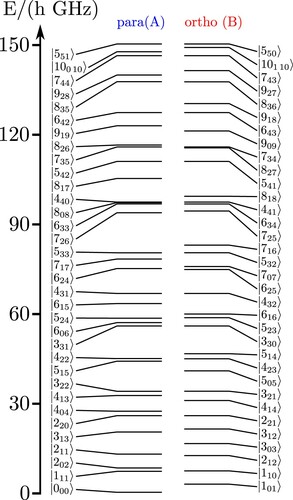
One can readily recognise close degeneracies of ortho and para levels allowing for nuclear spin symmetry mixing by hyperfine interactions. The usual selection rules for electric dipole transitions would be
(7)
(7)
(8)
(8)
and conservation of nuclear spin symmetry
(9)
(9)
where '↮' indicates a forbidden transition (rigorously forbidden if the approximation from Equation (Equation2
(2)
(2) ) is assumed).
If tunneling splittings were large as it may occur at very high vibrational or with electronic excitation, parity is a good quantum number and one has the parity selection rule (not relevant at low energy) for allowed electric dipole transitions (↔) with a change of parity.
(10)
(10)
2.3. Nuclear hyperfine hamiltonian, couplings and energy levels
If hyperfine effects are negligible and hyperfine splittings are not resolved as is frequently the case in infrared and visible spectra, the only effects from nuclear spin in the spectra arise from the nuclear spin statistical weights g in Tables and giving rise to intensity alternations in the corresponding line spectra [Citation46,Citation47]. When effects from the hyperfine energies are important, one has to include the coupling of the two quadrupolar nuclei and with rotation (Equation Equation4(4)
(4) ). So far only few cases of spectra with two coupled quadrupole nuclei have been analysed including the off diagonal interaction terms [Citation41,Citation78–81] and we follow in our analysis [Citation40,Citation77,Citation81] (see also [Citation82]). The program SPCAT of Pickett conveniently includes the possibility of important hyperfine effects from two quadrupolar nuclei and we have noted its power in such an analysis before [Citation81]. We have therefore used it in our calculations here as well, the parameters being taken from the analysis of [Citation40], summarised here in Table .
Table 5. Hyperfine constants for defined in Equation (Equation12
(12)
(12) ) with experimental values from Ref. [Citation40]. The two spin–rotation interaction terms
and
are 3 orders of magnitude smaller than the other parameters and our conclusions for the dynamics calculations are almost unchanged if these are set to zero. (For a definition of these, see Equations (S40, S41) in the supplementary of [Citation83] (see also [Citation82] for further discussion).
Briefly one has in Equation (Equation4(4)
(4) )
(11)
(11)
where N = 1 or 2 for the nucleus 1 or 2 of
and X, Y, Z are the space fixed coordinates and
is the nuclear quadrupole tensor operator related to the nuclear quadrupole moment
with
referring to the second derivative (with respect to X, Y, Z) of the electric potential at the position of the nucleus N. One finally introduces parameters for the quadrupole coupling
(12)
(12)
where α and β represent now the possible combinations of the principal axes a, b, c and e is the elementary charge (see also [Citation68,Citation81,Citation84]).
Introducing the notations used by Mizoguchi et al. [Citation40] and restricting attention to the isotopomer one couples first the two nuclear spins
(13)
(13)
followed by coupling of
to
giving a total angular momentum
(14)
(14)
The coupling of the angular momentum vectors
and
result in the triangular rules for the corresponding quantum numbers (in steps of 1)
(15)
(15)
(16)
(16)
One can now write the matrix elements of the nuclear spin Hamiltonian for two equal quadrupolar nuclei () in the symmetric basis functions with the coupling scheme presented in [Citation40]:
(17)
(17)
with the prefactor C
being given by
(18)
(18)
and with the Wigner 3-j symbol written with
and the 6-j symbol with
. As the quadrupole tensor in the principal axis system is symmetric the elements of the spherical quadrupole tensor for the two nuclei 1 and 2 (j = 1, 2) may be expressed as
(19)
(19)
Because the C
symmetry axis is the b-axis, we have the following symmetry relations between the quadrupole coupling constants for the two Cl-nuclei
(20)
(20)
Applying a Wang transformation to the matrix elements from Equation (Equation17
(17)
(17) ) gives the possibility to add the matrix elements from the A-reduced Watson Hamiltonian introduced in the previous section, which are usually also given in the Wang basis (see e.g. [Citation71–75]). We have reproduced the effective Hamiltonian from the program SPCAT [Citation77] for the given input parameters and have subsequently used the results for the eigenstate energies and for the dipole transition moments between the coupled basis functions from the output of SPCAT. For further details, we refer to the appendix.
Table provides a summary of all low energy hyperfine levels up to 40 GHz and a complete list up to 80 GHz is given in the supplementary tables. Besides the approximate assignment of the levels in terms of their dominant zero order contribution and the eigenstate energy we also indicate the contribution of ortho- and para states to the eigenstate (symbol ) and the two zero order states with the strongest contribution to the eigenstate (indicated by the symbol
in the appendix). It can be seen that all low energy states can be assigned as being either dominant ortho- or para-states by their nature (the 'forbidden weight' being typically less than 1%). The assignment by zero order quantum numbers is less unique, i.e. ‘intra-isomer mixings’ can be quite strong. But even the weak ortho-para mixings lead to observable ‘forbidden’ spectral lines as was shown experimentally [Citation42]. gives a graphical survey of the levels.
Figure 3. Low lying levels (below 25 GHz) for including all hyperfine levels separated into ‘para’ states (left) and ‘ortho’ states (right), and with splittings magnified.
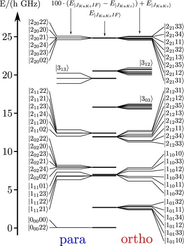
Table 6. Table of ortho–para coupling of all states with GHz with
and
with the simplified model ignoring the spin-rotation terms (see Equation (Equation3
(3)
(3) ) and appendix for more extensive tables. Here symbol E for energy/h).
Table contains a list of transition frequencies for the low frequency transitions including observed ‘forbidden’ ortho-para transitions from [Citation42] and the frequencies and intensities as calculated here from the simplified model. The agreement between the simplified model (parameters in Tables and and setting and
to zero) and the experiment is quite good, the root mean square deviation being
for the measured and calculated frequencies and the largest absolute deviation is
. Table gives a list of the calculated forbidden transitions and more complete tables are given in the supplementary publication.
Table 7. Table of ortho–para transitions ( above horizontal separation line from [Citation42] and below from [Citation40]) compared to the present calculation with
and the absolute square of the electric transition dipole matrix elements. The root mean square deviation is
.
Table 8. The strongest calculated ortho–para transitions using the simplified model and with for
sorted by intensity in decreasing order (see more complete table with
in the appendix).
In the present work, we study now the consequences for the time-dependent dynamics under radiative excitation.
2.4. Time-dependent dynamics of hyperfine states under coherent radiative excitation
We consider coherent radiative excitation of a molecular system () by coherent electromagnetic radiation under idealised conditions with negligible Doppler broadening in a cold molecular beam or a trap. The radiation field is assumed to be z-polarised with a slowly varying electric field amplitude envelope
represented by a quasiclassical electromagnetic wave propagating in the y-direction [Citation85–88]
(21)
(21)
is related to the microwave intensity I by the simple practical equation [Citation22]
(22)
(22)
The electric dipole approximation leads to an interaction energy
(23)
(23)
The time-dependent effective Hamiltonian for the molecule in the electromagnetic field is then (for a given position y of the molecule)
(24)
(24)
We have combined the phase factors into one phase η and omitted the explicit mentioning of y to simplify notation.
is the molecular Hamiltonian including hyperfine interactions as described in the previous sections. Following [Citation85–87], we derive the solution of the time-dependent Schrödinger equation for the molecule in the field
(25)
(25)
Expanding the wave function in the basis of molecular eigenstates
(in practice the rotational-hyperfine eigenstates given in Section 2.3 above) one has
(26)
(26)
Equation (Equation25
(25)
(25) ) then results in a matrix differential equation for the coefficients
(column matrix
, square Hamiltonian matrix
)
(27)
(27)
with diagonal elements of
being given by the eigenstates and off-diagonal elements in the electric dipole approximation
(28)
(28)
For slowly varying amplitude
, one can consider short intervals of time with constant
resulting in
(29)
(29)
leading to a set of coupled differential equations
(30)
(30)
with the diagonal matrix
. Applying the quasiresonant transformation [Citation88]
(31)
(31)
with the diagonal matrix
(32)
(32)
where
is the number of photons needed to reach near resonance
[Citation85–88] with small
one obtains with the neglect of small contributions from levels very far from resonance a matrix differential equation with a time-independent effective Hamiltonian matrix
(33)
(33)
where
and
(34)
(34)
is the same as
but setting explicitly all
for far-off-resonant couplings to zero.
For , one has the practical equation [Citation22]
(35)
(35)
The transition dipole matrix elements in Equation (Equation28
(28)
(28) ) were calculated with SPCAT [Citation77] from the eigenstate solutions in Section 2.3 including the hyperfine structure and taking as permanent dipole moment for ClSSCl the value
from [Citation42]. While, in principle, the treatment will include quasiresonant multiphoton transitions we have checked that for the conditions of the simulations reported below in the various excitations with different pulse sequences only multilevel systems in adjacent quasiresonant shells are coupled in practice. Also, for the conditions reported below, the quasiresonant approximation is excellent, as can be checked, for instance with the Floquet solutions using the URIMIR package, available when needed [Citation87] for more accurate solutions.
We also note that, in principle, magnetic dipole transitions could be included in essentially the same way, but they are orders of magnitude weaker and can be neglected (in contrast to the case of hyperfine structure excitation in Iodine, for instance [Citation87,Citation89,Citation90]). For further details and extensive derivations and discussion of the approximations, we refer to [Citation85–87,Citation91].
We have used this treatment for simulations of characteristic processes, which we have discussed before for the case of possible ortho–para transitions in simplified level schemes as shown in Figure . These include, in particular, the following processes:
Excitation of a nonstationary ‘chromophore’ para state
In a second process, one can start from a para state
In a third prototypical process, one can again start from a para state and excite it with a long pulse
Figure 4. Elementary level scheme for intramolecular couplings (not to scale). Pure para states are shown in the column above ‘para’, pure ortho states above ‘ortho’ and molecular eigenstates with contributions from both ortho- and para-states in the middle column (similar to Figure in [Citation22], where the otherwise self-explanatory notation is introduced).
![Figure 4. Elementary level scheme for intramolecular couplings (not to scale). Pure para states are shown in the column above ‘para’, pure ortho states above ‘ortho’ and molecular eigenstates with contributions from both ortho- and para-states in the middle column (similar to Figure 6 in [Citation22], where the otherwise self-explanatory notation is introduced).](/cms/asset/b6b2286f-1b3e-47bc-a251-31e2ac27fb9a/tmph_a_1959073_f0004_oc.jpg)
Figure 5. Level scheme for some low lying states of ClSSCl. Para states are shown in the column above ‘para’, ortho states above ‘ortho’ and selected eigenstates (symbol ) are shown in the middle. States denoted by the symbol
correspond to zero-order states of pure para and ortho character, whereas eigenstates are assigned as approximately para or ortho according to the dominant contribution (usually larger than
).
![Figure 5. Level scheme for some low lying states of ClSSCl. Para states are shown in the column above ‘para’, ortho states above ‘ortho’ and selected eigenstates (symbol |JKaKcIF〉) are shown in the middle. States denoted by the symbol |JKaKcIF] correspond to zero-order states of pure para and ortho character, whereas eigenstates are assigned as approximately para or ortho according to the dominant contribution (usually larger than 99%).](/cms/asset/6afd1eec-4e3c-4983-9c15-14a67fab2fa1/tmph_a_1959073_f0005_oc.jpg)
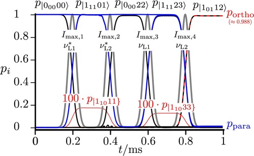
Figure 6. Sequential excitations starting from via
to
preparing
in the ground state and subsequent complete population transfer from para to ortho with
,
,
,
and all four pulse widths with
, the pulses being shown by the shaded gray lines. All frequencies are chosen to match exact resonances between the eigenstates.
We note that instead of generating a low-energy state with the pulse sequence and
, one can equivalently excite a high-energy superposition state of eigenstates of pure para and ortho characters (
) using the pulse sequence with frequencies
and
in the scheme of Figure , if such states can be identified at high energies. We might also mention that there exists a ‘folk myth’ among spectroscopists and others that such ‘exotic’ superpositions of ortho and para states cannot be prepared (e.g. [Citation93]), but as we have discussed before ([Citation22] and references cited therein) such superposition states are perfectly possible, as we shall demonstrate here for the case of the ‘real molecule’ ClSSCl.
Whereas we have reviewed these processes on simplified schemes before, the case of ClSSCl is the first example where such results can be demonstrated in a realistic hyperfine structure which corresponds to a much more complex multilevel situation of a real molecule.
Unless otherwise stated, in the simulations below all relevant levels in the multilevel system were included in the calculations, although explicit results for time-dependent state populations are given only for selected levels of particular importance. We should also note that in all simulations reported below we have used pure z-polarisation (with selection rule ) in the excitation, starting from an
initial state. Of course, similar simulations can be carried out for more general situations. We shall now discuss selected results for prototypical processes as they occur in ClSSCl.
3. Results for the time-dependent evolution
The effective Hamiltonian discussed in the previous section can be considered to be a satisfactory representation of the high resolution spectroscopic results reported in [Citation40–42]. Using the approach to the dynamics of coherent radiative excitation presented in Section 2.4, ClSSCl provides a unique opportunity to predict various time-dependent processes for para to ortho transitions, which we have reported in [Citation22] for a simplified model system as described by the elementary level scheme of Figure , but now extended to a completely realistic representation of an actual molecular system. We shall discuss the prototypical processes in turn for several selected aspects of the complex multilevel structures. As can be seen from Figure , these level structures occur as well-separated hyperfine structure ‘polyads’, where within each polyad there are many close-lying zero-order levels, which are coupled, subject to conservation of total angular momentum , to give a comparatively close lying set of eigenstates. The situation is reminiscent of the vibrational Fermi-resonance polyads in the vibrational spectra of polyatomic molecules, [Citation74,Citation94–96], but here on a very different energy scale. Because the polyads are very well separated in energy, coherent radiative excitation even with short, broadband, intense pulses will lead to dominant coupling just between pairs of two polyads at the given well-selected excitation frequencies. The excitation of other polyads is weak even though they are included in the calculation (within the quasiresonant approximation). The extensive tables in the appendix show however, that there are many ‘forbidden’ radiative transitions between ortho and para levels, which, while much weaker than the ‘allowed’ transitions, allow for substantial intercombinations between the ortho and para subsystems. We shall now discuss several exemplary cases.
3.1. Excitation in the low energy range: Coherent population transfer
Figure shows the low energy level diagram illustrating various possible excitation schemes following the elementary scheme of Figure . All levels are shown with their assignments, where we draw attention to the different energy scales on the ordinate and omitted energy ranges, where no extra levels occur between 100 kHz and 6760 MHz and the polyads ,
,
,
, and
have been omitted in the range from 6940 to 24758 MHz (see Figures and , each rotational level
giving rise to a set of close lying hyperfine levels with various possible values of I defining thus a ‘polyad’ in common spectroscopic nomenclature [Citation74]. When two or more rotational levels are close in energy, they also belong to the same polyad).
Within the different ranges, the representation of levels is to scale. We first demonstrate the paraortho transfer starting from a practically pure para state
(in the
notation) with also
and
due to the excitation with a long, moderately intense z-polarised pulse of high frequency purity. This generates a population transfer between eigenstates in the following sequence:
(36)
(36)
Figure shows the result for the time-dependent populations in these eigenstates. One can clearly see that this sequence leads to an almost complete population transfer from an essentially pure para state to an almost pure ortho state (with about 0.999988 ortho character in the eigenstate
).
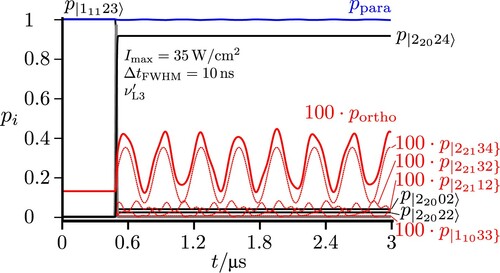
3.2. Short pulse excitation of a time-dependent para ‘chromophore’ state followed by para–ortho conversion in the isolated molecule
When one starts from the para ground state (with
prepared by the preceding steps as in Section 3.1) and excites with a relatively short, intense broad band pulse (
,
) one will excite initially a time-dependent ‘chromophore’ state of para character (symbolised by
in Figure and a dotted line to distinguish it from eigenstates), which is a superposition of the levels in the
polyad, corresponding in essence to a ‘zero-order’ state of the para isomer disregarding ortho–para coupling. After the end of the short pulse, there is an oscillatory exchange of population between the para and ortho isomers, in the isolated molecule, a purely intramolecular kinetic process. As the coupling is weak (
) and far off resonance the maximum population of the ortho isomer is only about 1% (magnified in Figure accordingly for better visibility). If there were only two levels involved as in the scheme of Figure , the population exchange would be simply periodic [Citation22]. Because of the more complex multilevel structures in the coupled
plus
polyad the oscillation of the populations appears as damped in Figure . We also show the dominant eigenstate populations in Figure , which are, of course, constant in time after the end of the pulse.
Figure 7. Excitation from the para ground state resonant to the ‘chromophore’ zero-order state estimated by the simplified scheme of two coupled states from [Citation22] (resulting here in the two eigenstates
and
). With a short pulse actually all hyperfine levels of the
and
polyads are excited simultaneously (frequency
). The lines in red correspond to projections with pure ortho character and in blue for pure para character. The total sum of populations of all states with pure para (or pure ortho) character is given by
and
. The dotted red lines show the projection of all eigenstates to the hyperfine levels
and
, with
representing the basis functions of the effective Hamiltonian with pure para or ortho character.
![Figure 7. Excitation from the para ground state resonant to the ‘chromophore’ zero-order state |11123] estimated by the simplified scheme of two coupled states from [Citation22] (resulting here in the two eigenstates |11123〉 and |11033〉). With a short pulse actually all hyperfine levels of the 111 and 110 polyads are excited simultaneously (frequency νL0=6766.4MHz). The lines in red correspond to projections with pure ortho character and in blue for pure para character. The total sum of populations of all states with pure para (or pure ortho) character is given by ppara and portho. The dotted red lines show the projection of all eigenstates to the hyperfine levels |11033} and |11011}, with |JKaKcIF} representing the basis functions of the effective Hamiltonian with pure para or ortho character.](/cms/asset/e15eb1b3-ed84-4ad9-96f4-4ab7e951d527/tmph_a_1959073_f0007_oc.jpg)
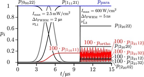
3.3. Preparation of an ‘exotic’ quantum superposition state of ortho and para isomers
As we have discussed in [Citation22], the scheme of Figure allows for the preparation of exotic superposition states of the different ortho and para nuclear spin symmetry isomers. This is similar to the preparation of exotic superpositions of structural isomers, such as enantiomers of chiral molecules [Citation23] or syn- and anti-isomers demonstrated in [Citation97] or, indeed, other kinds of structural isomers [Citation98,Citation99].
The molecular parameters of ClSSCl are such that no simple coherent radiative excitation scheme is available to generate superpositions of the lowest ortho and para states with the hypothetical sequence and
in Figure . However, such exotic superpositions can be generated at somewhat higher energy (
and
in Figures and ). In the scheme of Figure , one can first (with a long pulse of moderate intensity,
) excite an eigenstate
followed by an excitation of the polyad including
and
with a short intense pulse. The initial excitation of
follows the initial part of the sequence shown in Figure . The superposition of eigenstates after the last short pulse is shown in Figure to be dominated by the levels
,
and
, all of para character. However, also some states of mostly ortho character such as
are populated. If all of these eigenstates were either of pure para or pure ortho character the total para and ortho isomer population would be constant in time after the final pulse. However, in fact all these eigenstates carry also some of the ‘forbidden’ character of the opposite nuclear spin isomer. This results in a total population
after the pulse (shown in red and magnified for visibility) which oscillates around some non-zero average population near 0.25%.
Figure 8. Excitation from the para state with a frequency resonant to
. With this short pulse simultaneously all hyperfine levels of the
and
polyad are excited. The lines in red correspond to projections with pure ortho character and in blue for pure para character. Also
and
as defined in Figure are shown, with
magnified by a factor 100 for visibility. The lower red lines show the projection of all eigenstates to the hyperfine levels
,
and
, with
the basis functions of the effective Hamiltonian with pure para or ortho character.
A similar result is obtained when exciting with the long pulse initially the ‘para’ eigenstate followed by a broadband short pulse excitation into the
and
polyad. Figure shows again the constant eigenstate populations after the pulse (now dominantly
and
with some population carried by the ‘forbidden’ states
and
, magnified by 100 in the figure). The total ‘forbidden’ ortho population is again oscillating centred around a time averaged population a little less than 0.4%. While again this is not the simple result as it would be obtained from the idealised scheme in Figure , it nicely illustrates the exotic superposition of an exotic state which has ortho and para isomer nature at the same time. The reason for the relative large oscillations in the ortho population is, of course, that the eigenstates in the
and
polyad all have some contribution of the opposite ‘forbidden’ isomer. In order to find cases with smaller oscillation, one can look for eigenstates of a purer ortho and para character.
Figure 9. Resonant excitation from the para ground state via to
. With the second short pulse (frequency
), simultaneously all hyperfine levels of the
and
polyad are excited. The lines in red correspond to projections with pure ortho character and in blue for pure para character. The total sums of populations are given by
and
(see Figure ). The dotted red lines show the projection of all eigenstates to the hyperfine levels
and
, with
the basis functions of the effective Hamiltonian with pure para or ortho character.
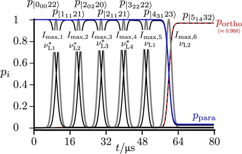
3.4. Excitation of higher polyads
As can be seen from the overview in Figure , the polyad structure with regions where ortho and para levels are either well separated or where the polyads include both ortho and para levels continues to higher rotational energies. Thus one can find levels with relatively pure ortho or para character and also levels where the eigenstates have substantial (although still minor) character of the respective ‘forbidden’ nuclear spin isomer. Figure shows examples with the well separated polyad of relatively pure ortho character and the polyad
(para), with ortho levels of
all falling in a range of about 3 MHz and therefore occur within the same polyad. Thus, after preparation of a para level, say, in the
polyad near
, by a suitable sequence of steps starting in the ground state, one can excite into the coupled polyad of
and
. If one selects then with a long pulse of moderate intensity and high frequency purity
an eigenstate
followed by an excitation with frequency
in Figure , on resonance with a ‘forbidden’ transition to
one can realise a transfer from an almost pure para state to an almost pure ortho state. Such a sequence is shown with selected pulses of similar length in Figure , describing the transitions:
(37)
(37)
before the final transfer to
.
Figure 10. Level scheme for some higher lying states of ClSSCl. Eigenstates assigned as dominantly para states are shown in the column above ‘para’, ortho states above ‘ortho’ and selected eigenstates with both para and ortho characters are shown in between (see also caption to Figure ).
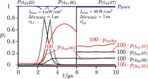
Figure 11. Sequential excitations starting from via
,
,
to
preparing the exemplary para to ortho population transfer from
via
to
with
,
,
,
,
and
and all six pulse widths
, with the pulses being shown by the shaded gray lines. All frequencies are chosen to match the exact resonances between the corresponding states. An almost complete population transfer to
and also to
) is reached.
Starting now from (
) considered as initial state in Figure , one can excite from there with a short (
) pulse a ‘chromophore’ state of almost pure para character. Such a state is dominantly a superposition of the eigenstates
and
, with some minor contribution from other eigenstates. If one analyses the superposition in terms of its time-dependent contributions from the pure para and pure ortho states one finds an oscillatory exchange between ortho and para isomers with a maximum contribution from the ortho isomer near 0.65 percent. It is instructive to compare this result, which is obtained when retaining essentially all hyperfine eigenstates in the description of the coherent radiative excitation with a result, which is obtained from a model such as in Figure where one para state as a lower state (with
) is radiatively coupled to only two excited eigenstates with
and
, which result from coupling two zero-order states of pure para (
) and pure ortho (
) character. This representative two coupled level model shows essentially the same ortho–para oscillation with a slightly larger amplitude (maximum near 0.85 percent for the ortho population). Thus for this selected example the simplified coupling model provides a reasonable semi-quantitative representation of the true, very complex multilevel situation. We also note that the ortho–para oscillation with a period of about
even in the complete multilevel dynamics appears as almost undamped, in contrast to the result in Figure .
Figure 12. Excitation from the higher lying para state with a frequency resonant to the 'chromophore' state (zero-order para state
estimated by the simplified scheme of two coupled states from [Citation22]). With a pulse of length
the eigenstates
and the ortho state
are excited. The lines in red correspond to projections with pure ortho character and in blue for pure para character. The total sum of all populations with para and ortho character is given by
and
. The dotted red line for
is identical to
, because only this ortho state is excited. In qualitative agreement with this we show
the time-dependent ortho population (full green line) from the simplified scheme of two coupled states from [Citation22] with
,
, a = 0.99934, b = 0.03633 and the reduced dipole transition moments chosen to eigenstates
and
in Figure with
and
.
![Figure 12. Excitation from the higher lying para state |32225〉 with a frequency resonant to the 'chromophore' state (zero-order para state |43126] estimated by the simplified scheme of two coupled states from [Citation22]). With a pulse of length 1μs the eigenstates |43126〉 and the ortho state |43236〉 are excited. The lines in red correspond to projections with pure ortho character and in blue for pure para character. The total sum of all populations with para and ortho character is given by ppara and portho. The dotted red line for p|43236} is identical to portho, because only this ortho state is excited. In qualitative agreement with this we show pno the time-dependent ortho population (full green line) from the simplified scheme of two coupled states from [Citation22] with W=4.5kHz, δ=123.5kHz, a = 0.99934, b = 0.03633 and the reduced dipole transition moments chosen to eigenstates Ψi and Ψn in Figure 4 with 〈Ψp|μ|Ψi〉=〈32225|μ|43126〉=1.792D and 〈Ψp|μ|Ψn〉=〈32225|μ|43236〉=−0.065D.](/cms/asset/0fc199d9-6080-415f-8b99-a17bc0bc8861/tmph_a_1959073_f0012_oc.jpg)
Figure shows the time evolution when one selects with a long pulse starting from the eigenstate
which has 99.75 percent para character and 0.25 percent ortho character. This first step is then followed by a short pulse excitation with a frequency
(cf. Figure ) resonant with the combined polyad of
and
in the range around
(cf. Figure and Figure ). As seen from Figure the final superposition of eigenstates is dominated by
and
(both largely para) but has a contribution of about 0.45 percent from
(largely ortho). Of course, the eigenstate populations after the pulse are constant in time. If one analyses the total wavefunction in the multilevel situation in terms of its time-dependent ortho and para characters, one has about 0.35 percent ortho character after the end of the short pulse, which is about constant in time. This example is therefore much closer to the simple scheme in Figure in its superposition state dynamics than the otherwise analogous example shown in Figure exciting into the combined
and
polyad. The time independence of the eigenstate populations does not imply a time-independent state. Rather, one has an oscillating state with a quasi-frequency of oscillation dominated by
(or a period
). This oscillation can be observed because of the time-dependent absorption spectrum of this time-dependent state, which we therefore have called a chameleon state (see [Citation22] and also [Citation98–100] and discussion in Section 2.4).
Figure 13. Excitation from the higher lying para state (
) with a frequency resonant to
(
) and subsequent simultaneous excitation of
(
) and
by a short pulse (
) resonant to
(
). With this the population from the eigenstate
is transferred to a superposition of eigenstates each of dominantly pure para and pure ortho character. A fraction of the population stays in
, which explains the difference between
and
.
3.5. Comparison with excitation by thermal radiation
It is instructive to compare the dynamics of nuclear spin isomer interconversion by coherent radiative transitions with the corresponding processes by collisions and by thermal background radiation. At ordinary pressures, collisional processes are obviously dominant and have in fact been studied in a number of cases ([Citation58–60] and references cited therein), although not for ClSSCl. However, here we consider experiments at very low pressures in molecular beams or traps, where collisional processes can be made negligible. Thermal background radiation can be made negligible as well by cooling the whole experimental setup to low temperatures (liquid nitrogen or liquid He [Citation23]). It is of interest, however, to study the processes more generally including room temperature conditions, where effects from thermal background radiation might become important under very low pressure conditions. This effect has been discussed in the more general context of thermal unimolecular reactions, where it was proposed to carry out the corresponding experiments under low pressure (molecular beam) conditions [Citation101], and these phenomena were subsequently studied experimentally and, indeed, publicised [Citation102]. As noted in [Citation85,Citation86,Citation101,Citation103], these processes have an interesting prehistory [Citation104].
The general rate coefficient expression for transitions from an initial state i to a final state f under thermal background radiation is given in [Citation101]
(38)
(38)
and
are the different energies of the initial and final levels in the transition and
for x>0 (x<0) (and 0 for x = 0, but the energies are assumed to be different in Equations (Equation38
(38)
(38) )–(Equation40
(40)
(40) )).
is the Einstein coefficient for spontaneous emission, which in the electric dipole approximation is given by Equation (Equation39
(39)
(39) )
(39)
(39)
From this one may derive the practically useful Equation (Equation40
(40)
(40) )
(40)
(40)
For microwave transitions at
the corresponding rate coefficients are on the order of
, which leads to negligible effects on the time scales considered here [Citation101]. However, as already discussed in the context of possible experiments on molecular parity violation [Citation23], at room temperature processes, which occur by radiative transitions to vibrationally excited states as intermediate levels, are much faster, typically with rate constants on the order of
for strongly allowed infrared transitions. We shall present here a simple model calculation for ClSSCl, for which infrared spectroscopic experiments with hyperfine structure resolution have not yet been reported. However, infrared vibrational spectra have been studied experimentally [Citation105] and by quantum chemical calculations [Citation106].
A strong vibrational band near has a calculated intensity
(or
), which corresponds to an absolute value of the vibrational transition moment
(see also [Citation84,Citation86]). In the absence of more detailed information, we shall compare the coherent radiative para
ortho conversion described in Figure to the simple scheme for infrared transitions by thermal radiation shown in Figure . This connects five levels of which four are dominantly ‘para’ in character and the final state 5 is dominantly ‘ortho’ in character. This is similar to Figure and to the transfer in Figure , but now with excitations occurring at infrared frequencies. For the transition intensities, we have taken the MW intensities scaled by the infrared frequencies and dipole moment (Equation Equation40
(40)
(40) ). Figure shows the time-dependent level populations starting with
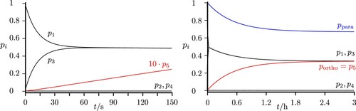
, as well as the total populations in the para- and ortho isomers. Transfer occurs and quasi-equilibrium is slowly reached on the time scale of milliseconds to seconds. For this particular process, which is just one example among a huge number of possible radiative transitions in the microwave and infrared range, quasi-equilibrium corresponds to about 30% final ortho-population given the selected subset of levels.
Figure 14. Simplified scheme for the paraortho transfer by thermal infrared transitions in a five-level system similar to the scheme shown in Figures and . We note that on a common energy scale, the levels 1, 3 and 5 on the one hand and 2 and 4 on the other hand are nearly degenerate (within
within one group of levels). Levels 1, 2, 3, 4 are dominantly para (
), level 5 is dominantly ortho. For
, the rate constants for the thermal transitions are
,
,
,
,
,
,
, and
, while ‘
’ indicates the rate constants for 2 and 4 shifted by
. The rate constants for all five states in the ground state are
,
,
,
,
,
,
,
and additionally
and
.
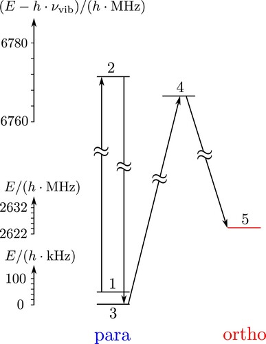
Figure 15. Time-dependent level populations for the simplified scheme of Figure under excitation with thermal background radiation at . The total populations in the para and ortho isomers are shown as well (with compressed time scale on the right hand side, see discussion in the text). If all levels were included, equilibrium would correspond to
ortho.
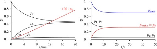
If one were to calculate all possible processes in the real ClSSCl molecule, one would obtain the statistical ortho/para ratio 10/6 according to the statistical weights (62.5% ortho). Figure shows also the corresponding level populations with incoherent thermal microwave radiation in a scheme exactly corresponding to Figures and . Here we have extended the time scale by factor of about . The present simple model estimates show, on what time scales for coherent radiative transfer one would have to cool the experimental setup to low temperatures and similar considerations apply to the experiment on parity violation [Citation23]. Figure shows the result for the ‘infrared’ scheme when exciting with thermal background radiation at
, the temperature of liquid Nitrogen.
Figure 16. Time-dependent level populations for the simplified scheme of Figure under excitation with thermal background radiation at with all five states belonging to the ground vibrational level (as in Figures and ). The total populations in the para and ortho isomers are shown as well (with compressed time scale on the right hand side, see discussion in the text). If all levels were included, equilibrium would correspond to
ortho.
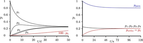
Figure 17. Time-dependent level populations for the simplified scheme of Figure under excitation with thermal background radiation at . The total populations in the para and ortho isomers are shown as well (with compressed time scale on the right hand side, see discussion in the text). If all levels were included, equilibrium would correspond to
ortho.
4. Discussion and conclusion
Parity and nuclear spin symmetry are approximate constants of the motion in quantum molecular dynamics, often assumed to correspond to almost exact symmetries [Citation44]. However, while the violation of parity symmetry is a very small effect, the interconversion of ‘parity isomers’ [Citation23] by collisional and radiative processes is facile [Citation39]. Nuclear spin symmetry isomers, on the other hand, are relatively stable with respect to collisions and radiation. The preparation and reaction dynamics of nuclear spin symmetry isomers have a long history starting with ortho- and para-hydrogen [Citation45–49]. Both the conservation of nuclear spin symmetry on short time scales and the interconversion between nuclear spin symmetry isomers under collisional conditions have been studied extensively [Citation44,Citation52–61]. The conservation of nuclear spin symmetry has been studied as well for reactive processes [Citation43,Citation57] and there have been recent demonstrations of different reactivities for nuclear spin symmetry isomers in bimolecular reactions [Citation107]. On the other hand, reaction dynamics with hyperfine structure resolution has been studied much less (see [Citation89,Citation90] for example) and direct observation of nuclear spin symmetry coupling by high resolution spectroscopy has been quite rare, with only a few examples, so far, in the literature (see [Citation108–113] and the reviews [Citation22,Citation44]). However, in principle, at very high excitations and high densities of rovibronic states in polyatomic molecules, the mixing of nuclear spin symmetry and even parity states must be ubiquitous on moderately long time scales of sub-ms to s [Citation44,Citation62,Citation63,Citation70]. For the common dissociated or ionised states resulting from different nuclear spin symmetry isomers the coupling is necessary and has, for instance, been made use of to determine in high precision spectroscopic experiments an accurate ground state interval between the ortho- and para-hydrogen isomers [Citation114,Citation115], although direct spectroscopic transitions between bound quantum states of ortho- and of para-hydrogen have not yet been observed. Such transitions have been observed in ,
and
, for example [Citation108–112].
Dichlorodisulfane ClSSCl is a unique example of a simple chiral molecule, where the parity violating energy difference between the ground state energies of the enantiomers has been studied by quantitative theory in relation to the hypothetical tunneling splitting in the parity conserving symmetrical case. In spite of the modest barrier (
) for interconversion between the enantiomers parity violation was shown to completely dominate the quantum dynamics at low energies, because of the minute tunneling splittings ([Citation36], recently reconfirmed [Citation116]). Parity symmetry is thus broken de lege in this molecule [Citation39]. Furthermore, most recent hyperfine structure resolved rotational spectra in the microwave range have demonstrated ‘forbidden’ transitions between the ortho- and para isomer manifolds [Citation42]. These observations have allowed us here to quantitatively predict the time-dependent processes of nuclear spin symmetry violation and compare them with the slower processes of intramolecular de lege parity violation for the first time in a realistic molecular example. We can summarise here some of the main conclusions from our investigation.
Already in the vibrational ground state, one can predict a very rich spectrum of ‘forbidden transitions’ connecting the ortho- and para-nuclear spin symmetry isomers. This allows us to study the time-dependent interconversion between the isomers by coherent radiative excitation.
The theoretical simulations demonstrate the possibility of an almost 100 percent complete transfer of population from an essentially pure para ground state to an almost pure excited ortho eigenstate on a collision-free time scale of less than 0.1 to
Short-pulse excitation from an almost pure para ground state to an excited time-dependent para chromophore state shows time-dependent intra-molecular (collision-free and radiationless) oscillatory interconversion between para and ortho nuclear spin isomers on a time scale of a few nanoseconds to a few microseconds. As the interconversion arises from a highly off-resonant coupling, the oscillation period is governed by the resonance defect and the maximum population transfer is 1 percent or less, typically, in these examples which should however, be easily detectable.
We have also demonstrated the preparation of exotic ‘chameleon states’, which are superpositions of eigenstates corresponding to ortho- and para- nuclear spin symmetry isomers. While the contributions from the isomers in the superposition state are not equal (0.5 and 99.5 percent typically, depending on the states chosen) they are in an experimentally detectable range, for instance by uncertainty limited frequency and time resolved spectroscopy [Citation89,Citation97].
We have furthermore shown that the transfer of population between para- and ortho-nuclear spin isomers by thermal radiation in the microwave range is exceedingly slow (up to 100 years at
In our modelling of various intramolecular and radiative transitions, we have neglected collisional effects. Such effects are expected to be small on the time scales considered and under typical molecular beam conditions and were shown to be negligibly small in the test experiments on NH under such conditions [Citation25]. One might possibly consider exotic very large collisional cross sections for decoherence of near degenerate levels. But even then one could optimise the experiments systematically to control the corresponding effects. We have also neglected magnetic dipole transitions which contribute very little in molecules like ClSSCl, although they can become important for systems with heavy atoms and could be included when needed [Citation87]. Similarly dynamic Stark effect type couplings can be assumed to result in small effects with the oscillatory fields considered, similar to the case of dynamic Zeeman-type splitting which were included explicitly in [Citation87].
In principle, all these effects and further small effects could be included in the calculations but are not expected to change any of the main results and conclusions significantly.
The time-dependent processes of nuclear spin symmetry isomerisation discussed here arise from couplings in complex multilevel structures arranged in rotational-nuclear spin state polyads. The conversion times observed here in the range between a few nanoseconds and a few microseconds can be interestingly compared to the times for intramolecular vibrational redistribution (IVR) which were derived from spectroscopy of complex Fermi-resonance polyads in polyatomic molecules to be as fast as 10 to [Citation16–20] but can also extend into the longer picosecond ranges for some molecules [Citation118–120]. An important aspect of the IVR processes discussed in [Citation16–20] and [Citation118–120] is the strong close resonance coupling observed for IVR, leading possibly to partial or complete microcanonical equilibrium-like distributions near to a partial maximum of entropy in a short time [Citation16–20,Citation98,Citation99,Citation121]. On the other hand, the weaker off resonant ortho-para coupling found in ClSSCl leads to a very incomplete redistribution of population (up to 1% only in the examples shown). However, one can anticipate that with excitation to high energy with high rovibrational densities of states, one can also obtain an effectively exponential relaxation towards microcanonical equilibrium between ortho and para isomers [Citation22,Citation62,Citation63,Citation70].
We can finally summarise some conclusions for possible future studies of parity violation in ClSSCl. The theoretically predicted corresponding to
[Citation36] falls in the range detectable by a current experimental setup [Citation25], using the approach of [Citation23]. The time scale for such an experiment is in the ms to second range, which is well separated from the much shorter times of nanoseconds to microseconds observed here for the interconversion of the nuclear spin symmetry isomers. This separation of time scales can be understood from the very different kind of symmetry breakings related to the two types of processes [Citation17,Citation22,Citation44,Citation91]. The separation of time scales corresponds to a comparable separation on the energy or frequency scale. The experimental approach using rovibrational frequency shifts could thus naturally be carried out on separate hyperfine structure states [Citation122–125] and the effect of hyperfine structure on parity violation can be studied theoretically by including nuclear spin-dependent terms [Citation34,Citation126], which lead to values
depending on the hyperfine structure level
(describing a rovibronic hyperfine level). Frequency shifts in MW or IR spectra, say [Citation37,Citation38,Citation65,Citation66], will then be
.
On the other hand, because parity does not change for different nuclear spin states, the time-dependent scheme [Citation23] to measure does not necessitate hyperfine resolution in order to detect an appropriate average value of
, because of the large separation of time scales. The separation of time scales will be less pronounced in molecules containing nuclear spin (1/2) nuclei. It remains true that the ideal choice of molecules for the study of parity violation would involve nuclei of spin 0 only (such as
S,
C or
O). Such molecules have been proposed, but they are difficult to synthesise [Citation39]. In that sense molecules with spin zero nuclei (S) and quadrupolar nuclei (Cl) only would be a ‘second best choice’. We might conclude with a speculation on the time scale of nuclear spin symmetry violation in molecules with zero nuclear spin. This would correspond to a change from a Pauli- allowed rovibronic state to rigorously Pauli forbidden state [Citation44]. Such states are usually considered to be nonexistent and have, indeed, never been observed. As we have discussed before [Citation44], their observation would correspond to a violation of a most fundamental symmetry principle in nature. There is, however, no experimental or theoretical evidence for such an effect.
Supplemental Material
Download PDF (365.2 KB)Acknowledgments
Our work was supported by an ERC Advanced grant and a generous grant from ETH Zürich. We enjoyed support and help from and many discussions with numerous coworkers and colleagues, and in particular Karen Keppler, Roberto Marquardt, Frédéric Merkt, Eduard Miloglyadov and Jürgen Stohner.
Disclosure statement
No potential conflict of interest was reported by the author(s).
Additional information
Funding
References
- J. Troe, Ber. Bunsenges. Phys. Chem. 73, 144–147 (1969).
- J. Troe, Ber. Bunsenges. Phys. Chem. 73, 906–911 (1969).
- J. Troe, Naturwissenschaften 56, 553–557 (1969). doi:https://doi.org/10.1007/BF00597258
- J. Troe, J. Phys. Chem. A 110, 2831–2849 (2006). doi:https://doi.org/10.1021/jp0680037
- J. Manz and L. Wöste, Femtosecond Chemistry, Proc. Berlin Conf. Femtosecond Chemistry, Berlin (March 1993), vols. 1 and 2, (Verlag Chemie, Weinheim, 1995).
- J. Troe, Ber. Bunsenges. Phys. Chem. 87, 161–169 (1983). doi:https://doi.org/10.1002/bbpc.19830870217
- J. Troe, J. Phys. Chem. 87, 1800–1804 (1983). doi:https://doi.org/10.1021/j100233a029
- H.J. Wörner and P. Corkum. Attosecond Spectroscopy, in Handbook of High-Resolution Spectroscopy, edited by M. Quack and F. Merkt (Wiley, Chichester, New York, 2011), Vol. 3, pp. 1781–1804.
- L. Gallmann and U. Keller. Femtosecond and Attosecond Light Sources and Techniques for Spectroscopy, in Handbook of High-Resolution Spectroscopy, edited by M. Quack and F. Merkt (Wiley, Chichester, New York, 2011), Vol. 3, pp. 1805–1836.
- L. Gallmann, J. Herrmann, R. Locher, M. Sabbar, A. Ludwig, M. Lucchini and U. Keller, Mol. Phys. 111, 2243–2250 (2013). doi:https://doi.org/10.1080/00268976.2013.799298
- A. Tehlar and H.J. Wörner, Mol. Phys. 111, 2057–2067 (2013). doi:https://doi.org/10.1080/00268976.2013.782439
- H. Braun, T. Bayer, M. Wollenhaupt and T. Baumert. 2D Strong-Field Spectroscopy to Elucidate Impulsive and Adiabatic Ultrafast Electronic Control Schemes in Molecules, in Molecular Spectroscopy and Quantum Dynamics, edited by R. Marquardt and M. Quack (Elsevier, 2020), pp. 79–112.
- D. Baykusheva and H.J. Wörner. Attosecond Molecular Dynamics and Spectroscopy, in Molecular Spectroscopy and Quantum Dynamics, edited by R. Marquardt and M. Quack (Elsevier, 2020), pp. 113–161.
- T. Ando, A. Iwasaki and K. Yamanouchi. Ultrafast Femtosecond Dynamics and High-Resolution Spectroscopy of Molecular Cations, in Molecular Spectroscopy and Quantum Dynamics, edited by R. Marquardt and M. Quack (Elsevier, 2020), pp. 283–300.
- F. Krausz and M. Ivanov, Rev. Mod. Phys. 81, 163–234 (2009). doi:https://doi.org/10.1103/RevModPhys.81.163
- R. Marquardt, M. Quack, J. Stohner and E. Sutcliffe, J. Chem. Soc. Farad. Trans. 2 82, 1173–1187 (1986). doi:https://doi.org/10.1039/f29868201173
- M. Quack, J. Mol. Struct. 292, 171–195 (1993). doi:https://doi.org/10.1016/0022-2860(93)80099-H
- M. Quack and J. Stohner, J. Phys. Chem. 97, 12574–12590 (1993). doi:https://doi.org/10.1021/j100150a020
- M. Quack, Chimia 55, 753–758 (2001).
- M. Quack. Molecular Femtosecond Quantum Dynamics between Less than Yoctoseconds and More than Days: Experiment and Theory, in Femtosecond Chemistry, Proc. Berlin Conf. Femtosecond Chemistry, (March 1993), edited by J. Manz and L. Wöste (Verlag Chemie, Berlin, 1995), Chap. 27, pp. 781–818.
- K. Bergmann, H.C. Nägerl, C. Panda, G. Gabrielse, E. Miloglyadov, M. Quack, G. Seyfang, G. Wichmann, S. Ospelkaus, A. Kuhn, S. Longhi, A. Szameit, P. Pirro, B. Hillebrands, X.F. Zhu, J. Zhu, M. Drewsen, W.K. Hensinger, S. Weidt, T. Halfmann, H.L. Wang, G.S. Paraoanu, N.V. Vitanov, J. Mompart, T. Busch, T.J. Barnum, D.D. Grimes, R.W. Field, M.G. Raizen, E. Narevicius, M. Auzinsh, D. Budker, A. Pálffy and C.H. Keitel, J. Phys. B At. Mol. Opt. Phys. 52, 202001 (2019). doi:https://doi.org/10.1088/1361-6455/ab3995(Roadmap on STIRAP applications, Chapter A2.3 Precision experiments for parity violation in chiral molecules: the role of STIRAP, E. Miloglyadov, M. Quack, G. Seyfang, G. Wichmann, pp. 11–13).
- M. Quack, G. Seyfang and G. Wichmann, Adv. Quant. Chem. 81, 51–104 (2020). doi:https://doi.org/10.1016/bs.aiq.2020.06.001
- M. Quack, Chem. Phys. Lett. 132, 147–153 (1986). doi:https://doi.org/10.1016/0009-2614(86)80098-7
- M. Quack and G. Seyfang. Tunnelling and Parity Violation in Chiral and Achiral Molecules: Theory and High Resolution Spectroscopy, in Tunnelling in Molecules: Nuclear Quantum Effects from Bio to Physical Chemistry, edited by J. Kästner, and D. Kozuch (Royal Society of Chemistry, Cambridge, England, 2020), pp. 192–244.
- P. Dietiker, E. Miloglyadov, M. Quack, A. Schneider and G. Seyfang, J. Chem. Phys. 143, 244305 (2015). doi:https://doi.org/10.1063/1.4936912
- A. Ryle, F. Sanger, L. Smith and R. Kitai, Biochem. J. 60, 541–556 (1955). doi:https://doi.org/10.1042/bj0600541(and references therein).
- F.M. Bickelhaupt, M. Solà and P.v.R. Schleyer, J. Comp. Chem. 16, 465–477 (1995). doi:https://doi.org/10.1002/jcc.v16:4 (and references therein).
- G. Winnewisser, M. Winnewisser and W. Gordy, J. Chem. Phys. 49, 3465 (1968). doi:https://doi.org/10.1063/1.1670621
- G. Winnewisser, Vibr. Spectrosc. 8, 241–253 (1995). doi:https://doi.org/10.1016/0924-2031(94)00053-J6th Austrian-Hungarian International Conference on Vibrational Spectroscopy.
- R. Martín-Doménech, I. Jiménez-Serra, G.M. Muñoz Caro, H.S.P. Müller, A. Occhiogrosso, L. Testi, P.M. Woods and S. Viti, Astron. Astrophys. 585, A112, 1–9 (2016).
- C. Zhu, S. Góbi, M.J. Abplanalp, R. Frigge, J.J. Gillis-Davis and R.I. Kaiser, J. Geophys. Res. Planets 124, 2772–2779 (2019). doi:https://doi.org/10.1029/2018JE005913
- M. Gottselig, D. Luckhaus, M. Quack, J. Stohner and M. Willeke, Helvet. Chim. Acta 84, 1846–1861 (2001). doi:https://doi.org/10.1002/(ISSN)1522-2675
- A. Bakasov and M. Quack, Chem. Phys. Lett. 303, 547–557 (1999). doi:https://doi.org/10.1016/S0009-2614(99)00238-9
- R. Berger and M. Quack, J. Chem. Phys. 112, 3148–3158 (2000). doi:https://doi.org/10.1063/1.480900
- L. Horný and M. Quack, Mol. Phys. 113, 1768–1779 (2015). doi:https://doi.org/10.1080/00268976.2015.1012131
- R. Berger, M. Gottselig, M. Quack and M. Willeke, Angew. Chem. Int. Ed. 40, 4195–4198 (2001). doi:https://doi.org/10.1002/1521-3773(20011119)40:22¡¿1.0.CO;2-D. Angew. Chem. 113, pp. 4342–4345 (2001).
- M. Quack and J. Stohner, Phys. Rev. Lett. 84, 3807–3810 (2000). doi:https://doi.org/10.1103/PhysRevLett.84.3807
- M. Quack and J. Stohner, J. Chem. Phys. 119, 11228–11240 (2003). doi:https://doi.org/10.1063/1.1622381
- M. Quack, Angew. Chem., Int. Edit. 28, 571–586 (1989). doi:https://doi.org/10.1002/(ISSN)1521-3773. Angew. Chem. 101, 588–604 (1989).
- A. Mizoguchi, S. Ota, H. Kanamori, Y. Sumiyoshi and Y. Endo, J. Mol. Spectr. 250, 86–97 (2008). doi:https://doi.org/10.1016/j.jms.2008.04.012
- Z.T. Dehghani, S. Ota, A. Mizoguchi and H. Kanamori, J. Phys. Chem. A 117, 10041–10046 (2013). doi:https://doi.org/10.1021/jp400632g
- H. Kanamori, Z.T. Dehghani, A. Mizoguchi and Y. Endo, Phys. Rev. Lett. 119, 173401 (2017). doi:https://doi.org/10.1103/PhysRevLett.119.173401
- M. Quack, Mol. Phys. 34, 477–504 (1977). doi:https://doi.org/10.1080/00268977700101861
- M. Quack. Fundamental Symmetries and Symmetry Violations from High Resolution Spectroscopy, in Handbook of High Resolution Spectroscopy, edited by M. Quack and F. Merkt (Wiley, Chichester, New York, 2011), Vol. 1, Chap. 18, pp. 659–722.
- E.P. Wigner, Z. Physik. Chem. B23, 28–32 (1933).
- G. Herzberg, Molecular spectra and molecular structure; I. Spectra of Diatomic Molecules, (D. van Nostrand Company, Inc., Princeton, New Jersey, New York, 1950), (First edition in German: Molekülspektren und Molekülstruktur; I. Zweiatomige Moleküle, T.Steinkopff Verlag Dresden und Leipzig, 1939).
- F. Hund, Z. Physik 42, 93–120 (1927). doi:https://doi.org/10.1007/BF01397124
- K.F. Bonhoeffer and P. Harteck, Z. Physik. Chem. 4B, 113–141 (1929). doi:https://doi.org/10.1515/zpch-1929-0408
- L. Farkas, in Book series: Ergebnisse der exakten Naturwissenschaften, (Springer Berlin Heidelberg, Berlin, Heidelberg, 1933), Chap. 6, pp. 163–218.
- S. Albert, I. Bolotova, Z. Chen, C. Fábri, L. Horný, M. Quack, G. Seyfang and D. Zindel, Phys. Chem. Chem. Phys. 18, 21976–21993 (2016). doi:https://doi.org/10.1039/C6CP01493C
- S. Albert, I. Bolotova, Z. Chen, C. Fabri, M. Quack, G. Seyfang and D. Zindel, Phys. Chem. Chem. Phys. 19, 11738–11743 (2017). doi:https://doi.org/10.1039/C7CP01139C
- B.J. Orr, Mol. Phys. 116, 3666–3700 (2018). doi:https://doi.org/10.1080/00268976.2018.1490463
- A. Amrein, M. Quack and U. Schmitt, J. Phys. Chem. 92, 5455–5466 (1988). doi:https://doi.org/10.1021/j100330a025
- C. Manca Tanner, M. Quack and D. Schmidiger, Mol. Phys. 116, 3718–3730 (2018). doi:https://doi.org/10.1080/00268976.2018.1484952(and references therein).
- V. Horká-Zelenková, G. Seyfang, P. Dietiker and M. Quack, J. Phys. Chem. A 123, 6160–6174 (2019). doi:https://doi.org/10.1021/acs.jpca.9b02580(and references therein).
- G. Wichmann, E. Miloglyadov, G. Seyfang and M. Quack, Mol. Phys. 118, e1752946 (2020). doi:https://doi.org/10.1080/00268976.2020.1752946
- M. Cordonnier, D. Uy, R.M. Dickson, K.E. Kerr, Y. Zhang and T. Oka, J. Chem. Phys. 113, 3181–3193 (2000). doi:https://doi.org/10.1063/1.1285852
- R.F. Curl, J.V.V. Kasper and K.S. Pitzer, J. Chem. Phys. 46, 3220–3228 (1967). doi:https://doi.org/10.1063/1.1841193
- K. Bahloul, M. Irac-Astaud, E. Ilisca and P.L. Chapovsky, J. Phys. B At. Mol. Opt. Phys. 31, 73–85 (1998). doi:https://doi.org/10.1088/0953-4075/31/1/010
- P.L. Chapovsky and L.J.F. Hermans, Ann. Rev. Phys. Chem. 50, 315–345 (1999). doi:https://doi.org/10.1146/annurev.physchem.50.1.315
- T. Oka. Orders of Magnitude and Symmetry in Molecular Spectroscopy, in Handbook of High Resolution Spectroscopy, edited by M. Quack and F. Merkt (Wiley, Chichester, New York, 2011).
- M. Quack, Farad. Disc. 102, 90–93 (1995). 358–360.
- M. Quack, Comments on intramolecular dynamics and femtosecond kinetics, Proc. 20th Solvay Conference Chemical reactions and their control on the femtosecond time scale, Adv. Chem. Phys., 1997, 101, 83–84, 92–93, 202, 277–278, 282, 373–388, 443, 453–456, 459, 586–591, 595.
- C.J. Marsden, R.D. Brown and P.D. Godfrey, J. Chem. Soc., Chem. Commun. 00, 399–401 (1979). doi:https://doi.org/10.1039/c39790000399
- M. Quack and J. Stohner, Z. Phys. Chem. 214, 675–703 (2000). doi:https://doi.org/10.1524/zpch.2000.214.5.675
- M. Quack and J. Stohner. How Do Parity Violating Weak Nuclear Interactions Inuence Rovibrational Frequencies in Chiral Molecules? in SASP 2000, Proceedings of the XII Symposium on Atomic and Surface Physics and Related Topics, edited by D. Bassi and P. Tosi, P (Univ. di Trento, Folgaria, Italy, 2000), pp. PR–11, 1–4.
- H.C. Longuet-Higgins, Mol. Phys. 6, 445–460 (1963). doi:https://doi.org/10.1080/00268976300100501
- A. Bauder. Fundamentals of Rotational Spectroscopy, in Handbook of High-resolution Spectroscopy, edited by M. Quack and F. Merkt (Wiley, Chichester, New York, 2011).
- M. Hippler, E. Miloglyadov, M. Quack and G. Seyfang. Mass and Isotope Selective Infrared Spectroscopy, in Handbook of High Resolution Spectroscopy, edited by M. Quack and F. Merkt (Wiley, Chichester; New York, 2011), Vol. 2, Chap. 28, pp. 1069–1118.
- M. Quack, J. Chem. Phys. 82, 3277–3283 (1985). doi:https://doi.org/10.1063/1.448225
- J.K.G. Watson, in Vibrational Spectra and Structure, edited by J. Durig (1977), Vol. 6, pp. 1.
- D. Papoušek and M.R. Aliev, in Molecular Vibrational / Rotational Spectra, 1982.
- R.N. Zare, Angular Momentum (John Wiley & Sons Inc., New York, 1988).
- S. Albert, K. Keppler Albert, H. Hollenstein, C. Manca Tanner and M. Quack. Fundamentals of Rotation-Vibration Spectra, in Handbook of High-Resolution Spectroscopy; Fundamentals of Rotation-Vibration Spectra, edited by M. Quack and F. Merkt (Wiley, Chichester, New York, 2011), Vol. 1, Chap. 3, pp. 117–173.
- H. Kroto, Molecular Rotation Spectra (Wiley, London, 1975).
- D. Luckhaus and M. Quack, Mol. Phys. 68, 745–758 (1989). doi:https://doi.org/10.1080/00268978900102511
- H.M. Pickett, J. Mol. Spectr. 148, 371–377 (1991). doi:https://doi.org/10.1016/0022-2852(91)90393-O
- H.S.P. Müller and M.C.L. Gerry, J. Chem. Soc., Faraday Trans. 90, 3473–3481 (1994). doi:https://doi.org/10.1039/FT9949003473
- W.H. Flygare and W.D. Gwinn, J. Chem. Phys. 36, 787–794 (1962). doi:https://doi.org/10.1063/1.1732611
- M.R. Keenan, D.B. Wozniak and W.H. Flygare, J. Chem. Phys. 75, 631–640 (1981). doi:https://doi.org/10.1063/1.442080
- A. Bauder, A. Beil, D. Luckhaus, F. Müller and M. Quack, J. Chem. Phys. 106, 7558–7570 (1997). doi:https://doi.org/10.1063/1.473759
- H. Benz, A. Bauder and H. Günthard, J. Mol. Spectr. 21, 156–164 (1966). doi:https://doi.org/10.1016/0022-2852(66)90134-2
- P. Yu and N.R. Hutzler, Phys. Rev. Lett. 126, 023003 (2021). doi:https://doi.org/10.1103/PhysRevLett.126.023003
- E.R. Cohen, T. Cvitas, J.G. Frey, B. Holmström, K. Kuchitsu, R. Marquardt, I. Mills, F. Pavese, M. Quack, J. Stohner, H.L. Strauss, M. Takami and A.J. Thor, Quantities, Units and Symbols in Physical Chemistry 3rd ed (IUPAC and Royal Society of Chemistry RSC Publishing, Cambridge, 2007).
- M. Quack, J. Chem. Phys. 69, 1282–1307 (1978). doi:https://doi.org/10.1063/1.436667
- F. Merkt and M. Quack. Molecular Quantum Mechanics and Molecular Spectra, Molecular Symmetry, and Interaction of Matter with Radiation, in Handbook of High-Resolution Spectroscopy; Molecular Quantum Mechanics and Molecular Spectra, Molecular Symmetry, and Interaction of Matter with Radiation, edited by Quack, M. and Merkt, F. (Wiley, Chichester, New York, 2011), Vol. 1, Chap. 1, pp. 1–55.
- R. Marquardt, M. Quack, J. Stohner and I. Thanopulos, Mol. Phys. 117, 3132–3147 (2019). doi:https://doi.org/10.1080/00268976.2019.1606952(with 537 pages of supplementary material including URIMIR package FORTRAN code).
- M. Quack. Reaction Dynamics and Statistical Mechanics of the Preparation of Highly Excited States by Intense Infrared Radiation, in Advances in Chemical Physics, edited by K. Lawley, I. Prigogine and S.A. Rice (John Wiley and Sons, Chichester and New York, 1982), Vol. 50, pp. 395–473.
- Y.B. He, J. Pochert, M. Quack, R. Ranz and G. Seyfang, Farad. Discuss. 102, 275–300 (1995). doi:https://doi.org/10.1039/fd9950200275
- T.K. Ha, Y. He, J. Pochert, M. Quack, R. Ranz, G. Seyfang and I. Thanopoulos, Ber. Bunsenges. Phys. Chem. 99, 384–392 (1995). doi:https://doi.org/10.1002/bbpc.v99:3
- R. Marquardt and M. Quack. Foundations of Time Dependent Quantum Dynamics of Molecules under Isolation and in Coherent Electromagnetic Fields, in Molecular Spectroscopy and Quantum Dynamics, edited by R. Marquardt and M. Quack 1st ed (Elsevier, Amsterdam, 2020).
- E. Schrödinger, Naturwissenschaften 23, 807–812 (1935). doi:https://doi.org/10.1007/BF01491891823–828, 844–849.
- T. Grohmann and J. Manz, Mol. Phys. 116, 2538–2555 (2018). doi:https://doi.org/10.1080/00268976.2018.1473651
- H.R. Dübal and M. Quack, Mol. Phys. 53, 257–264 (1984). doi:https://doi.org/10.1080/00268978400102271
- V. Horká, M. Quack and M. Willeke, Mol. Phys. 106, 1303–1316 (2008). doi:https://doi.org/10.1080/00268970802275611
- M. Quack, Ann. Rev. Phys. Chem. 41, 839–874 (1990). doi:https://doi.org/10.1146/annurev.pc.41.100190.004203
- C. Fábri, S. Albert, Z. Chen, R. Prentner and M. Quack, Phys. Chem. Chem. Phys. 20, 7387–7394 (2018). doi:https://doi.org/10.1039/C8CP00133B
- M. Quack. Die Symmetrie von Zeit und Raum und ihre Verletzung in molekularen Prozessen, in Jahrbuch 1990-1992 der Akademie der Wissenschaften zu Berlin (W. de Gruyter Verlag, Berlin, 1993), pp. 467–507.
- M. Quack. The Symmetries of Time and Space and Their Violation in Chiral Molecules and Molecular Processes, in Conceptual Tools for Understanding Nature. Proc. 2nd Int. Symp. of Science and Epistemology Seminar, Trieste April 1993, edited by Costa, G., Calucci, G. and Giorgi, M. (World Scientific Publ., Singapore, 1995), pp. 172–208.
- M. Quack, Europ. Rev. 22, S50–S86 (2014). doi:https://doi.org/10.1017/S106279871300077X
- M. Quack, Ber. Bunsenges. Phys. Chem. 83, 757–775 (1979). doi:https://doi.org/10.1002/bbpc.v83:8
- R.C. Dunbar and T.B. McMahon, Science 279, 194–197 (1998). doi:https://doi.org/10.1126/science.279.5348.194
- M. Quack, Farad. Discuss. Chem. Soc. 150, 533–565 (2011). doi:https://doi.org/10.1039/c1fd00096a
- J. Perrin, Trans. Faraday Soc. 17, 546–572 (1922). doi:https://doi.org/10.1039/tf9221700546(Discussion on the Radiation Theory of Chemical Action and references therein).
- S.G. Frankiss, J. Mol. Struct. 2, 271–279 (1968). doi:https://doi.org/10.1016/0022-2860(68)80019-5
- D. Das and S.L. Whittenburg, J. Phys. Chem. A 103, 2134–2140 (1999). doi:https://doi.org/10.1021/jp984210y
- A. Kilaj, H. Gao, D. Rösch, U. Rivero, J. Küpper and S. Willitsch, Nature Comm. 9, 00–0 (2018). doi:https://doi.org/10.1038/s41467-018-04483-3
- P. Yi, I. Ozier and N.F. Ramsey, J. Chem. Phys. 55, 5215–5227 (1971). doi:https://doi.org/10.1063/1.1675660
- J. Bordé, C.J. Bordé, C. Salomon, A. Van Lerberghe, M. Ouhayoun and C.D. Cantrell, Phys. Rev. Lett. 45, 14–17 (1980). doi:https://doi.org/10.1103/PhysRevLett.45.14
- J.P. Pique, F. Hartmann, R. Bacis, S. Churassy and J.B. Koffend, Phys. Rev. Lett. 52, 267–270 (1984). doi:https://doi.org/10.1103/PhysRevLett.52.267
- A.D.J. Critchley, A.N. Hughes and I.R. McNab, Phys. Rev. Lett. 86, 1725–1728 (2001). doi:https://doi.org/10.1103/PhysRevLett.86.1725
- A.D.J. Critchley, A.N. Hughes, I.R. McNab and R.E. Moss, Mol. Phys. 101, 651–661 (2003). doi:https://doi.org/10.1080/0026897021000021886
- K. Tanaka, M. Hayashi, M. Ohtsuki, K. Harada and T. Tanaka, Mol. Phys. 108, 2289–2301 (2010). doi:https://doi.org/10.1080/00268971003685764
- D. Sprecher, M. Beyer and F. Merkt, Mol. Phys. 111, 2100–2107 (2013). doi:https://doi.org/10.1080/00268976.2013.788743
- M. Beyer, N. Hölsch, J. Hussels, C.F. Cheng, E.J. Salumbides, K.S.E. Eikema, W. Ubachs, C. Jungen and F. Merkt, Phys. Rev. Lett. 123, 163002 (2019). doi:https://doi.org/10.1103/PhysRevLett.123.163002
- N. Sahu, J. Richardson and R. Berger, J. Comput. Chem. 42, 210–221 (2021). doi:https://doi.org/10.1002/jcc.v42.4
- P.L. Chapovsky, MNRAS 503, 1773–1779 (2020). doi:https://doi.org/10.1093/mnras/stab407
- K. von Puttkamer, H.R. Dübal and M. Quack, Farad. Discuss. Chem. Soc. 75, 197–210 (1983). doi:https://doi.org/10.1039/DC9837500197
- A. Kushnarenko, E. Miloglyadov, M. Quack and G. Seyfang, Phys. Chem. Chem. Phys. 20, 10949–10959 (2018). doi:https://doi.org/10.1039/C7CP08561C
- R. Marquardt and M. Quack. Energy Redistribution in Reacting Systems, in Encyclopedia of Chemical Physics and Physical Chemistry, edited by J.H. Moore and N. Spencer (IOP publishing, Bristol, 2001), Vol. 1 (Fundamentals), chap. A. 3.13, pp. 897–936.
- M. Quack, Nova. Acta. Leopold. 81, 137–173 (1999).
- V. Letokhov, Phys. Lett. A 53, 275–276 (1975). doi:https://doi.org/10.1016/0375-9601(75)90064-X
- C. Daussy, T. Marrel, A. Amy-Klein, C.T. Nguyen, C.J. Bordé and C. Chardonnet, Phys. Rev. Lett. 83, 1554–1557 (1999). doi:https://doi.org/10.1103/PhysRevLett.83.1554
- S.K. Tokunaga, C. Stoeffler, F. Auguste, A. Shelkovnikov, C. Daussy, A. Amy-Klein, C. Chardonnet and B. Darqui, Mol. Phys. 111, 2363–2373 (2013). doi:https://doi.org/10.1080/00268976.2013.821186
- A. Cournol, M. Manceau, M. Pierens, L. Lecordier, D.B.A. Tran, R. Santagata, B. Argence, A. Goncharov, O. Lopez, M. Abgrall, Y.L. Coq, R.L. Targat, H.A. Martinez, W.K. Lee, D. Xu, P.E. Pottie, R.J. Hendricks, T.E. Wall, J.M. Bieniewska, B.E. Sauer, M.R. Tarbutt, A. Amy-Klein, S.K. Tokunaga and B. Darquié, Quantum. Elec. (Woodbury) 49, 288–292 (2019). doi:https://doi.org/10.1070/QEL16880
- F. Hobi, R. Berger and J. Stohner, Mol. Phys. 111, 2345–2362 (2013). doi:https://doi.org/10.1080/00268976.2013.816444
Appendix
In the electronic supplementary material, we include the following documents and tables:
Description of the input used for the SPCAT program.
Table A1: Complete extended list of calculated rotational levels for the model (complete list related to Table )
Table A2: Complete extended list of hyperfine structure levels calculated from the model (complete list related to Table extended to high energies). This list contains also the contributions from the most important basis states in the last few columns (see discussion in the text)
Table A3: Complete list of the strongest ortho-para transitions with
Table A4: Energy levels (on diagonal, E/h in MHz) and transition dipole matrix elements (in D) for the calculations in Figure .
Table A5: Energy levels (on diagonal, E/h in MHz) and transition dipole matrix elements (in D) for the calculations in Figure .
Table A6: Energy levels (on diagonal, E/h in MHz) and transition dipole matrix elements (in D) for the calculations in Figure .
Table A7: Energy levels (on diagonal, E/h in MHz) and transition dipole matrix elements (in D) for the calculations in Figure .
Table A8: Energy levels (on diagonal, E/h in MHz) and transition dipole matrix elements (in D) for the calculations in Figure .
Table A9: Energy levels (on diagonal, E/h in MHz) and transition dipole matrix elements (in D) for the calculations in Figure .
Table A10: Energy levels (on diagonal, E/h in MHz) and transition dipole matrix elements (in D) for the calculations in Figure .
Table A11–A17: Extended results corresponding to Tables A4–A10 including all levels retained in the calculations.