Calculation of reaction rate constants from a classical Wigner model based on a Feynman path integral open polymer

Abstract

The Open Polymer Classical Wigner (OPCW) method [J. Chem. Phys. 152, 094111 (2020)] is applied to a flux-Heaviside trace for calculating reaction rate constants. The obtained expression for the reaction rate constant is tested on a symmetric Eckart potential. The OPCW method is shown to converge toward the exact classical Wigner result. The OPCW method shows some promise for rate constant calculations and suggestions for future tests are made.

GRAPHICAL ABSTRACT

KEYWORDS:

• Reaction rate constant
• open polymer classical Wigner model
• flux-side correlation function

1. Introduction

Reaction rates are of central importance in chemistry and methods to calculate reaction rate constants are therefore of interest. In many cases classical mechanics is sufficient in order to calculate rate constants, but quantum mechanics can be essential for instance for light atoms, such as hydrogen, and in cold environments.

Methods to obtain reaction rate constants from a Wigner distribution include the classical Wigner method [1, 2], with alternatives such as Feynman–Kleinert Linearised Path Integral [3] (FK-LPI), Local Gaussian Approximation Linearised Semi-Classical Initial Value Representation [4] (LGA-LSC-IVR), and to some extent the transition state theory with quantum partition functions of Wigner [5] and Eyring [6] and the quantum transition state theory of Pollak and Liao [7]. Other notable approximate quantum mechanical methods to calculate reaction rate constants are e.g. the instanton reaction rate theory [8–10], the statistical adiabatic channel model [11] and Ring Polymer Molecular Dynamics (RPMD) [12].

This article presents reaction rate constant calculations using a recent implementation of the classical Wigner method by the same authors [13]. Section 2 is an introduction to a general formulation of chemical reaction rates, then section 3 combines this theory with the Open Polymer Classical Wigner (OPCW) method. Section 4 notes some important corrections to consider for running the calculations. Sections 5, 6, and 7 respectively give the details of the computations that have been run, show the results of these computations, and contain the conclusions that have been drawn.

2. Reaction rate constants

Miller and coworkers published three quantum mechanical traces that can be used to acquire bimolecular reaction rate constants [14, 15]. These traces are (1) $\begin{array}{rl}{C}_{\mathrm{s}\mathrm{s}}\left(t\right)& =\mathrm{T}\mathrm{r}\left\{{\text{e}}^{-\frac{\text{β}}{2}\hat{H}}h\left(-\hat{x}\right){\text{e}}^{-\frac{\text{β}}{2}\hat{H}}{\text{e}}^{\frac{\mathrm{i}\hat{H}t}{\hslash }}h\left(\hat{x}\right){\text{e}}^{-\frac{\mathrm{i}\hat{H}t}{\hslash }}\right\}\end{array}$(1) (2) $\begin{array}{rl}{C}_{\mathrm{f}\mathrm{s}}\left(t\right)& =\mathrm{T}\mathrm{r}\left\{{\text{e}}^{-\frac{\text{β}}{2}\hat{H}}\hat{F}{\text{e}}^{-\frac{\text{β}}{2}\hat{H}}{\text{e}}^{\frac{\mathrm{i}\hat{H}t}{\hslash }}h\left(\hat{x}\right){\text{e}}^{-\frac{\mathrm{i}\hat{H}t}{\hslash }}\right\}\end{array}$(2) (3) $\begin{array}{rl}{C}_{\mathrm{f}\mathrm{f}}\left(t\right)& =\mathrm{T}\mathrm{r}\left\{{\text{e}}^{-\frac{\text{β}}{2}\hat{H}}\hat{F}{\text{e}}^{-\frac{\text{β}}{2}\hat{H}}{\text{e}}^{\frac{\mathrm{i}\hat{H}t}{\hslash }}\hat{F}{\text{e}}^{-\frac{\mathrm{i}\hat{H}t}{\hslash }}\right\}\end{array}$(3) where $h\left(x\right)$ is the Heaviside function, $\hat{x}$ is the position operator, $\text{β}=(k_{\mathrm{B}}T{)}^{-1}$, where $k_{\mathrm{B}}$ is Boltzmann's constant and T is the absolute temperature, $\hat{H}$ is the Hamiltonian operator of the system, i is the imaginary unit, t is time, ℏ is the reduced Planck constant, and $\hat{F}$ is the probability density flux operator. These functions can be used to obtain reaction rate constants, $k_{\mathrm{r}}$, through the relations (4) $\begin{array}{rl}{k}_{\mathrm{r}}{Q}_{\mathrm{R}}& =\underset{t\to \mathrm{\infty }}{lim}\frac{\text{d}}{\text{d}t}{C}_{\mathrm{s}\mathrm{s}}\left(t\right)\end{array}$(4) (5) $\begin{array}{rl}& =\underset{t\to \mathrm{\infty }}{lim}{C}_{\mathrm{f}\mathrm{s}}\left(t\right)\end{array}$(5) (6) $\begin{array}{rl}& ={\int }_0^{\mathrm{\infty }}\text{d}t{C}_{\mathrm{f}\mathrm{f}}\left(t\right)=\frac{1}{2}{\int }_{-\mathrm{\infty }}^{\mathrm{\infty }}\text{d}t{C}_{\mathrm{f}\mathrm{f}}\left(t\right)\end{array}$(6)

where $Q_{\mathrm{R}}$ is the canonical partition function per unit volume of the reactants.

It can be noted that the traces presented here have a symmetrised Boltzmann operator [16], i.e. ${\text{e}}^{-\frac{\text{β}}{2}\hat{H}}$ on both sides of the first operator in each trace. The relations 4(4) $\begin{array}{rl}{k}_{\mathrm{r}}{Q}_{\mathrm{R}}& =\underset{t\to \mathrm{\infty }}{lim}\frac{\text{d}}{\text{d}t}{C}_{\mathrm{s}\mathrm{s}}\left(t\right)\end{array}$(4) – 6(6) $\begin{array}{rl}& ={\int }_0^{\mathrm{\infty }}\text{d}t{C}_{\mathrm{f}\mathrm{f}}\left(t\right)=\frac{1}{2}{\int }_{-\mathrm{\infty }}^{\mathrm{\infty }}\text{d}t{C}_{\mathrm{f}\mathrm{f}}\left(t\right)\end{array}$(6) are just as valid for the real part of the trace with an asymmetrically placed Boltzmann operator [14]. Important to notice is that these relations are defined for potentials where the reactants start infinitely far from each other and the products end up infinitely far from each other. This requires the potential to be unbound. This restriction applies to the potential employed in this article. In the computations presented in this article the trace used for the calculation of rate constants is $C_{\mathrm{f}\mathrm{s}}\left(t\right)$.

3. Reaction rate constant calculation with the open polymer classical wigner method

In this section expressions for calculating reaction rate constants with the OPCW method will be derived. These derivations follow the ones in the original OPCW article [13] quite closely, but use the symmetrised Boltzmann operator and will be specialised to the flux-side trace, $C_{\text{fs}}\left(t\right)$ in Equation 2(2) $\begin{array}{rl}{C}_{\mathrm{f}\mathrm{s}}\left(t\right)& =\mathrm{T}\mathrm{r}\left\{{\text{e}}^{-\frac{\text{β}}{2}\hat{H}}\hat{F}{\text{e}}^{-\frac{\text{β}}{2}\hat{H}}{\text{e}}^{\frac{\mathrm{i}\hat{H}t}{\hslash }}h\left(\hat{x}\right){\text{e}}^{-\frac{\mathrm{i}\hat{H}t}{\hslash }}\right\}\end{array}$(2) .

Initially $C_{\text{fs}}\left(t\right)$ is written as the integral over position, $x_1$, of a matrix element. (7) $C_{\text{fs}}\left(t\right)={\int }_{-\mathrm{\infty }}^{\mathrm{\infty }}\text{d}{x}_1〈x_1\left|{\text{e}}^{-\frac{\text{β}}{2}\hat{H}}\hat{F}{\text{e}}^{-\frac{\text{β}}{2}\hat{H}}{\text{e}}^{\frac{\mathrm{i}\hat{H}t}{\hslash }}h\left(\hat{x}\right){\text{e}}^{-\frac{\mathrm{i}\hat{H}t}{\hslash }}\right|x_1〉$(7)

The Boltzmann operators are each divided into $\frac{N}{2}$ factors of ${\text{e}}^{-\frac{\text{β}}{N}\hat{H}}$, where N must be an even number. N−1 identity operators are inserted between these operators. (8) $\begin{array}{rl}{C}_{\text{fs}}\left(t\right)& =\left\{\prod _{j=1}^N{\int }_{-\mathrm{\infty }}^{\mathrm{\infty }}\text{d}{x}_j\right\}〈x_1\left|{\text{e}}^{-\frac{\text{β}}{N}\hat{H}}\right|x_2〉〈x_2\left|{\text{e}}^{-\frac{\text{β}}{N}\hat{H}}\right|x_3〉\\ & \dots 〈x_{\frac{N}{2}}\left|{\text{e}}^{-\frac{\text{β}}{N}\hat{H}}\hat{F}\right|x_{\frac{N}{2}+1}〉\\ & \dots 〈x_{N-1}\left|{\text{e}}^{-\frac{\text{β}}{N}\hat{H}}\right|x_N〉\\ & \times 〈x_N\left|{\text{e}}^{-\frac{\text{β}}{N}\hat{H}}{\text{e}}^{\frac{\mathrm{i}\hat{H}t}{\hslash }}h\left(\hat{x}\right){\text{e}}^{-\frac{\mathrm{i}\hat{H}t}{\hslash }}\right|x_1〉\end{array}$(8) This is an imaginary time, $-\mathrm{i}\hslash \text{β}$, Feynman path integral [17], which can be expressed with Wigner transforms instead of matrix elements, (9) $\begin{array}{rl}{C}_{\text{fs}}\left(t\right)& =\left\{\prod _{j=1}^N{\iint }_{-\mathrm{\infty }}^{\mathrm{\infty }}\frac{\text{d}{x}_j\text{d}{p}_j}{2\pi \hslash }\right\}{\text{e}}^{-\frac{\mathrm{i}}{\hslash }\sum _{j=1}^N{p}_j\left(x_{\left(jmodN\right)+1}-x_j\right)}\\ & \times {\left({\text{e}}^{-\frac{\text{β}}{N}\hat{H}}\right)}_{\text{W}}\left[\frac{x_1+x_2}{2},p_1\right]\\ & \times {\left({\text{e}}^{-\frac{\text{β}}{N}\hat{H}}\right)}_{\text{W}}\left[\frac{x_2+x_3}{2},p_2\right]\\ & \dots {\left({\text{e}}^{-\frac{\text{β}}{N}\hat{H}}\hat{F}\right)}_{\text{W}}\left[\frac{x_{\frac{N}{2}}+x_{\frac{N}{2}+1}}{2},p_{\frac{N}{2}}\right]\\ & \dots {\left({\text{e}}^{-\frac{\text{β}}{N}\hat{H}}\right)}_{\text{W}}\left[\frac{x_{N-1}+x_N}{2},p_{N-1}\right]\\ & \times {\left({\text{e}}^{-\frac{\text{β}}{N}\hat{H}}{\text{e}}^{\frac{\mathrm{i}\hat{H}t}{\hslash }}h\left(\hat{x}\right){\text{e}}^{-\frac{\mathrm{i}\hat{H}t}{\hslash }}\right)}_{\text{W}}\left[\frac{x_N+x_1}{2},p_N\right].\end{array}$(9) In the limit $N\to \mathrm{\infty }$ the Wigner transform of the Boltzmann operator simplifies to the classical Boltzmann factor. Also, the Boltzmann operators can be separated from the flux and Heaviside operators in this limit. We obtain (10) $\begin{array}{rl}{C}_{\text{fs}}\left(t\right)& =\underset{N\to \mathrm{\infty }}{lim}\left\{\prod _{j=1}^N{\iint }_{-\mathrm{\infty }}^{\mathrm{\infty }}\frac{\text{d}{x}_j\text{d}{p}_j}{2\pi \hslash }\right\}\\ & \times {\text{e}}^{-\frac{\mathrm{i}}{\hslash }\sum _{j=1}^N{p}_j\left(x_{\left(jmodN\right)+1}-x_j\right)}\\ & \times {\text{e}}^{-\frac{\text{β}}{N}\sum _{j=1}^{N}H\left(y_j,p_j\right)}{\left(\hat{F}\right)}_{\text{W}}\left[y_{\frac{N}{2}},p_{\frac{N}{2}}\right]\\ & \times {\left({\text{e}}^{\frac{\mathrm{i}\hat{H}t}{\hslash }}h\left(\hat{x}\right){\text{e}}^{-\frac{\mathrm{i}\hat{H}t}{\hslash }}\right)}_{\text{W}}\left[y_N,p_N\right]\end{array}$(10) where $y_j=\frac{x_j+x_{\left(jmodN\right)+1}}{2}$ and $H(y_j,p_j)$ is the classical Hamiltonian. If $V\left(y_j\right)$ is independent of momentum, all momenta except $p_{\frac{N}{2}}$ and $p_N$ can be integrated out analytically as done in the original derivation of the OPCW method [13]. This gives (11) $\begin{array}{rl}{C}_{\text{fs}}\left(t\right)& =\underset{N\to \mathrm{\infty }}{lim}{\left(\frac{mN}{2\pi \text{β}}\right)}^{\frac{N}{2}}\frac{\text{β}}{2\pi mN}{\hslash }^{-N}\left\{\prod _{j=1}^N{\int }_{-\mathrm{\infty }}^{\mathrm{\infty }}\text{d}{x}_j\right\}\\ & \times {\iint }_{-\mathrm{\infty }}^{\mathrm{\infty }}\text{d}{p}_{\frac{N}{2}}\text{d}{p}_N{\text{e}}^{-\frac{\text{β}}{N}\sum _{j=1}^{N}V\left(y_j\right)}\\ & \times {\text{e}}^{-\frac{mN}{2{\hslash }^2\text{β}}\left(\sum _{j=1}^{\frac{N}{2}-1}{\left(x_{j+1}-x_j\right)}^2+\sum _{j=\frac{N}{2}+1}^{N-1}{\left(x_{j+1}-x_j\right)}^2\right)}\\ & \times {\text{e}}^{-\frac{\mathrm{i}}{\hslash }{p}_{\frac{N}{2}}\left(x_{\frac{N}{2}+1}-x_{\frac{N}{2}}\right)}{\text{e}}^{-\frac{\text{β}}{N}\frac{p_{\frac{N}{2}}^2}{2m}}{\left(\hat{F}\right)}_{\text{W}}\left[y_{\frac{N}{2}},p_{\frac{N}{2}}\right]\\ & \times {\text{e}}^{-\frac{\mathrm{i}}{\hslash }{p}_N\left(x_1-x_N\right)}{\text{e}}^{-\frac{\text{β}}{N}\frac{p_N^2}{2m}}\\ & \times {\left({\text{e}}^{\frac{\mathrm{i}\hat{H}t}{\hslash }}h\left(\hat{x}\right){\text{e}}^{-\frac{\mathrm{i}\hat{H}t}{\hslash }}\right)}_{\text{W}}\left[y_N,p_N\right],\end{array}$(11) where m is the mass. For the flux operator $\hat{F}=\frac{1}{2m}\left(\delta \right(\hat{x})\hat{p}+\hat{p}\delta (\hat{x}\left)\right)$, the Wigner transform is (12) ${\left(\hat{F}\right)}_{\text{W}}\left[x,p\right]=\frac{p}{m}\delta \left(x\right),$(12) where $\delta \left(x\right)$ is the Dirac delta function. Using the momentum integrals of Appendix A in our previous article [13] a quantity $F^{\prime }(y_{\frac{N}{2}},x_{\frac{N}{2}+1}-x_{\frac{N}{2}})$ can be defined as (13) $\begin{array}{rl}{F}^{\prime }\left(y_{\frac{N}{2}},x_{\frac{N}{2}+1}-x_{\frac{N}{2}}\right)& =\frac{{\int }_{-\mathrm{\infty }}^{\mathrm{\infty }}\text{d}{p}_{\frac{N}{2}}{\left(\hat{F}\right)}_{\text{W}}\left[y_{\frac{N}{2}},p_{\frac{N}{2}}\right]{\text{e}}^{-\frac{\text{β}}{N}\frac{p_{\frac{N}{2}}^2}{2m}}{\text{e}}^{-\frac{\mathrm{i}}{\hslash }{p}_{\frac{N}{2}}\left(x_{\frac{N}{2}+1}-x_{\frac{N}{2}}\right)}}{{\int }_{-\mathrm{\infty }}^{\mathrm{\infty }}\text{d}{p}_{\frac{N}{2}}{\text{e}}^{-\frac{\text{β}}{N}\frac{p_{\frac{N}{2}}^2}{2m}}{\text{e}}^{-\frac{\mathrm{i}}{\hslash }{p}_{\frac{N}{2}}\left(x_{\frac{N}{2}+1}-x_{\frac{N}{2}}\right)}}\\ & =\frac{{\int }_{-\mathrm{\infty }}^{\mathrm{\infty }}\text{d}{p}_{\frac{N}{2}}\frac{p_{\frac{N}{2}}}{m}\delta \left(y_{\frac{N}{2}}\right){\text{e}}^{-\frac{\text{β}}{N}\frac{p_{\frac{N}{2}}^2}{2m}}{\text{e}}^{-\frac{\mathrm{i}}{\hslash }{p}_{\frac{N}{2}}\left(x_{\frac{N}{2}+1}-x_{\frac{N}{2}}\right)}}{\sqrt{\frac{2\pi mN}{\text{β}}}{\text{e}}^{-\frac{\text{β}}{N}\frac{m{N}^2{\left(x_{\frac{N}{2}+1}-x_{\frac{N}{2}}\right)}^2}{2{\hslash }^2{\text{β}}^2}}}\\ & =-\frac{\mathrm{i}N}{\hslash \text{β}}\left(x_{\frac{N}{2}+1}-x_{\frac{N}{2}}\right)\delta \left(y_{\frac{N}{2}}\right).\end{array}$(13)

This can be put into Equation 11(11) $\begin{array}{rl}{C}_{\text{fs}}\left(t\right)& =\underset{N\to \mathrm{\infty }}{lim}{\left(\frac{mN}{2\pi \text{β}}\right)}^{\frac{N}{2}}\frac{\text{β}}{2\pi mN}{\hslash }^{-N}\left\{\prod _{j=1}^N{\int }_{-\mathrm{\infty }}^{\mathrm{\infty }}\text{d}{x}_j\right\}\\ & \times {\iint }_{-\mathrm{\infty }}^{\mathrm{\infty }}\text{d}{p}_{\frac{N}{2}}\text{d}{p}_N{\text{e}}^{-\frac{\text{β}}{N}\sum _{j=1}^{N}V\left(y_j\right)}\\ & \times {\text{e}}^{-\frac{mN}{2{\hslash }^2\text{β}}\left(\sum _{j=1}^{\frac{N}{2}-1}{\left(x_{j+1}-x_j\right)}^2+\sum _{j=\frac{N}{2}+1}^{N-1}{\left(x_{j+1}-x_j\right)}^2\right)}\\ & \times {\text{e}}^{-\frac{\mathrm{i}}{\hslash }{p}_{\frac{N}{2}}\left(x_{\frac{N}{2}+1}-x_{\frac{N}{2}}\right)}{\text{e}}^{-\frac{\text{β}}{N}\frac{p_{\frac{N}{2}}^2}{2m}}{\left(\hat{F}\right)}_{\text{W}}\left[y_{\frac{N}{2}},p_{\frac{N}{2}}\right]\\ & \times {\text{e}}^{-\frac{\mathrm{i}}{\hslash }{p}_N\left(x_1-x_N\right)}{\text{e}}^{-\frac{\text{β}}{N}\frac{p_N^2}{2m}}\\ & \times {\left({\text{e}}^{\frac{\mathrm{i}\hat{H}t}{\hslash }}h\left(\hat{x}\right){\text{e}}^{-\frac{\mathrm{i}\hat{H}t}{\hslash }}\right)}_{\text{W}}\left[y_N,p_N\right],\end{array}$(11) , giving (14) $\begin{array}{rl}{C}_{\text{fs}}\left(t\right)& =\underset{N\to \mathrm{\infty }}{lim}{\left(\frac{mN}{2\pi \text{β}}\right)}^{\frac{N}{2}}\sqrt{\frac{\text{β}}{2\pi mN}}{\hslash }^{-N}\left\{\prod _{j=1}^N{\int }_{-\mathrm{\infty }}^{\mathrm{\infty }}\text{d}{x}_j\right\}\\ & \times {\int }_{-\mathrm{\infty }}^{\mathrm{\infty }}\text{d}{p}_N{\text{e}}^{-\frac{\text{β}}{N}\sum _{j=1}^{N}V\left(y_j\right)}\\ & \times {\text{e}}^{-\frac{mN}{2{\hslash }^2\text{β}}\sum _{j=1}^{N-1}{\left(x_{j+1}-x_j\right)}^2}\\ & \times \frac{\mathrm{i}N}{\hslash \text{β}}\left(x_{\frac{N}{2}}-x_{\frac{N}{2}+1}\right)\delta \left(y_{\frac{N}{2}}\right)\\ & \times {\text{e}}^{-\frac{\mathrm{i}}{\hslash }{p}_N\left(x_1-x_N\right)}{\text{e}}^{-\frac{\text{β}}{N}\frac{p_N^2}{2m}}\\ & \times {\left({\text{e}}^{\frac{\mathrm{i}\hat{H}t}{\hslash }}h\left(\hat{x}\right){\text{e}}^{-\frac{\mathrm{i}\hat{H}t}{\hslash }}\right)}_{\text{W}}\left[y_N,p_N\right].\end{array}$(14) We apply the classical Wigner approximation, (15) $\begin{array}{rl}& {\left({\text{e}}^{\frac{\mathrm{i}\hat{H}t}{\hslash }}h\left(\hat{x}\right){\text{e}}^{-\frac{\mathrm{i}\hat{H}t}{\hslash }}\right)}_{\text{W}}\left[y_N,p_N\right]\\ & \approx {\left(h\left(\hat{x}\right)\right)}_{\text{W}}\left[x\left(y_N,p_N,t\right),p\left(y_N,p_N,t\right)\right]\\ & =h\left(x\left(y_N,p_N,t\right)\right),\end{array}$(15) where $x(y_N,p_N,t)$ is the position at time t of a classical trajectory starting from $y_N$ and $p_N$. Then, by assuming finite N, we obtain (16) $\begin{array}{rl}{C}_{\text{fs},y}\left(t\right)& \approx {\left(\frac{mN}{2\pi \text{β}}\right)}^{\frac{N}{2}}\sqrt{\frac{\text{β}}{2\pi mN}}{\hslash }^{-N}\\ & \times \left\{\prod _{j=1}^N{\int }_{-\mathrm{\infty }}^{\mathrm{\infty }}\text{d}{x}_j\right\}{\int }_{-\mathrm{\infty }}^{\mathrm{\infty }}\text{d}{p}_N{\text{e}}^{-\frac{\mathrm{i}}{\hslash }{p}_N\left(x_1-x_N\right)}\\ & \times {\text{e}}^{-\frac{\text{β}}{N}\left(\frac{p_N^2}{2m}+\sum _{j=1}^{N}V\left(y_j\right)+\frac{m{N}^2}{2{\hslash }^2{\text{β}}^2}\sum _{j=1}^{N-1}{\left(x_{j+1}-x_j\right)}^2\right)}\\ & \times \frac{\mathrm{i}N}{\hslash \text{β}}\left(x_{\frac{N}{2}}-x_{\frac{N}{2}+1}\right)\delta \left(y_{\frac{N}{2}}\right)h\left(x\left(y_N,p_N,t\right)\right),\end{array}$(16) which is the expression corresponding to the $y_1$-version of the OPCW method for the flux-Heaviside trace. Due to the symmetrisation of the Boltzmann operator, the expression contains $y_{\frac{N}{2}}$ rather than $y_1$ and below it is simply referred to as the y-version of the OPCW method. The trace will be called $C_{\text{fs},y}\left(t\right)$. As shown in Appendix 1, we can also formulate an alternative version of the flux-Heaviside trace where the delta function now takes $x_{\frac{N}{2}}$ as argument. This results in: (17) $\begin{array}{rl}{C}_{\text{fs},x}\left(t\right)& \approx {\left(\frac{mN}{2\pi \text{β}}\right)}^{\frac{N}{2}}\sqrt{\frac{\text{β}}{2\pi mN}}{\hslash }^{-N}\left\{\prod _{j=1}^N{\int }_{-\mathrm{\infty }}^{\mathrm{\infty }}\text{d}{x}_j\right\}\\ & \times {\int }_{-\mathrm{\infty }}^{\mathrm{\infty }}\text{d}{p}_N{\text{e}}^{-\frac{\mathrm{i}}{\hslash }{p}_N\left(x_1-x_N\right)}\\ & \times {\text{e}}^{-\frac{\text{β}}{N}\left(\frac{p_N^2}{2m}+\sum _{j=1}^{N}V\left(y_j\right)+\frac{m{N}^2}{2{\hslash }^2{\text{β}}^2}\sum _{j=1}^{N-1}{\left(x_{j+1}-x_j\right)}^2\right)}\\ & \times \left(\frac{\mathrm{i}\hslash \text{β}}{4Nm}\left(\frac{\text{d}V\left(y_{\frac{N}{2}}\right)}{\text{d}{y}_{\frac{N}{2}}}+\frac{\text{d}V\left(y_{\frac{N}{2}+1}\right)}{\text{d}{y}_{\frac{N}{2}+1}}\right)\right.\\ & +\left.\phantom{\frac{\text{d}V\left(y_{\frac{N}{2}+1}\right)}{\text{d}{y}_{\frac{N}{2}+1}}}\frac{\mathrm{i}N}{2\hslash \text{β}}\left(x_{\frac{N}{2}}-x_{\frac{N}{2}+2}\right)\right)\delta \left(x_{\frac{N}{2}+1}\right)\\ & \times h\left(x\left(y_N,p_N,t\right)\right),\end{array}$(17) which below is called the x-version of the OPCW method for the flux-Heaviside trace.

4. Correction factors for evaluation of traces with monte carlo

In this work the position integrals in Equations 16(16) $\begin{array}{rl}{C}_{\text{fs},y}\left(t\right)& \approx {\left(\frac{mN}{2\pi \text{β}}\right)}^{\frac{N}{2}}\sqrt{\frac{\text{β}}{2\pi mN}}{\hslash }^{-N}\\ & \times \left\{\prod _{j=1}^N{\int }_{-\mathrm{\infty }}^{\mathrm{\infty }}\text{d}{x}_j\right\}{\int }_{-\mathrm{\infty }}^{\mathrm{\infty }}\text{d}{p}_N{\text{e}}^{-\frac{\mathrm{i}}{\hslash }{p}_N\left(x_1-x_N\right)}\\ & \times {\text{e}}^{-\frac{\text{β}}{N}\left(\frac{p_N^2}{2m}+\sum _{j=1}^{N}V\left(y_j\right)+\frac{m{N}^2}{2{\hslash }^2{\text{β}}^2}\sum _{j=1}^{N-1}{\left(x_{j+1}-x_j\right)}^2\right)}\\ & \times \frac{\mathrm{i}N}{\hslash \text{β}}\left(x_{\frac{N}{2}}-x_{\frac{N}{2}+1}\right)\delta \left(y_{\frac{N}{2}}\right)h\left(x\left(y_N,p_N,t\right)\right),\end{array}$(16) and 17(17) $\begin{array}{rl}{C}_{\text{fs},x}\left(t\right)& \approx {\left(\frac{mN}{2\pi \text{β}}\right)}^{\frac{N}{2}}\sqrt{\frac{\text{β}}{2\pi mN}}{\hslash }^{-N}\left\{\prod _{j=1}^N{\int }_{-\mathrm{\infty }}^{\mathrm{\infty }}\text{d}{x}_j\right\}\\ & \times {\int }_{-\mathrm{\infty }}^{\mathrm{\infty }}\text{d}{p}_N{\text{e}}^{-\frac{\mathrm{i}}{\hslash }{p}_N\left(x_1-x_N\right)}\\ & \times {\text{e}}^{-\frac{\text{β}}{N}\left(\frac{p_N^2}{2m}+\sum _{j=1}^{N}V\left(y_j\right)+\frac{m{N}^2}{2{\hslash }^2{\text{β}}^2}\sum _{j=1}^{N-1}{\left(x_{j+1}-x_j\right)}^2\right)}\\ & \times \left(\frac{\mathrm{i}\hslash \text{β}}{4Nm}\left(\frac{\text{d}V\left(y_{\frac{N}{2}}\right)}{\text{d}{y}_{\frac{N}{2}}}+\frac{\text{d}V\left(y_{\frac{N}{2}+1}\right)}{\text{d}{y}_{\frac{N}{2}+1}}\right)\right.\\ & +\left.\phantom{\frac{\text{d}V\left(y_{\frac{N}{2}+1}\right)}{\text{d}{y}_{\frac{N}{2}+1}}}\frac{\mathrm{i}N}{2\hslash \text{β}}\left(x_{\frac{N}{2}}-x_{\frac{N}{2}+2}\right)\right)\delta \left(x_{\frac{N}{2}+1}\right)\\ & \times h\left(x\left(y_N,p_N,t\right)\right),\end{array}$(17) are evaluated with Metropolis Monte Carlo [18]. In Monte Carlo integration there is a weight function and an integrand. Here, the weight function used is (18) $\begin{array}{rl}& {\left(\frac{mN}{2\pi \text{β}}\right)}^{\frac{N}{2}}\sqrt{\frac{\text{β}}{2\pi mN}}{\hslash }^{-N}\\ & \times {\text{e}}^{-\frac{\text{β}}{N}\left(\frac{p_N^2}{2m}+\sum _{j=1}^{N}V\left(y_j\right)+\frac{m{N}^2}{2{\hslash }^2{\text{β}}^2}\sum _{j=1}^{N-1}{\left(x_{j+1}-x_j\right)}^2\right)}\delta \left(y_{y,x}\right),\end{array}$(18) where $y_{y,x}$ is either $y_{\frac{N}{2}}$ or $x_{\frac{N}{2}+1}$. The integrand is thus (19) ${\text{e}}^{-\frac{\mathrm{i}}{\hslash }{p}_N\left(x_1-x_N\right)}\frac{\mathrm{i}N}{\hslash \text{β}}\left(x_{\frac{N}{2}}-x_{\frac{N}{2}+1}\right)h\left(x\left(y_N,p_N,t\right)\right)$(19) for the y-version of the OPCW method and (20) $\begin{array}{rl}& {\text{e}}^{-\frac{\mathrm{i}}{\hslash }{p}_N\left(x_1-x_N\right)}\\ & \times \left(\frac{\mathrm{i}\hslash \text{β}}{4Nm}\left(\frac{\text{d}V\left(y_{\frac{N}{2}}\right)}{\text{d}{y}_{\frac{N}{2}}}+\frac{\text{d}V\left(y_{\frac{N}{2}+1}\right)}{\text{d}{y}_{\frac{N}{2}+1}}\right)\right.\\ & +\left.\phantom{\frac{\text{d}V\left(y_{\frac{N}{2}+1}\right)}{\text{d}{y}_{\frac{N}{2}+1}}}\frac{\mathrm{i}N}{2\hslash \text{β}}\left(x_{\frac{N}{2}}-x_{\frac{N}{2}+2}\phantom{\frac{\text{β}{z}^{\text{β}}{N}_{\gamma ,k}\left({\mu }_{k}z\right)}{{\mu }_k^2}}\right)\right)\\ & \times h\left(x\left(y_N,p_N,t\right)\right)\end{array}$(20) for the x-version of the OPCW method. This means that the quantity actually calculated is $\frac{C_{\text{fs}}\left(t\right)}{Z_{\delta }^{\prime }}$, where $Z_{\delta }^{\prime }$ is (21) $\begin{array}{rl}{Z}_{\delta }^{\prime }& ={\left(\frac{mN}{2\pi \text{β}}\right)}^{\frac{N}{2}}\sqrt{\frac{\text{β}}{2\pi mN}}{\hslash }^{-N}\left\{\prod _{j=1}^N{\int }_{-\mathrm{\infty }}^{\mathrm{\infty }}\text{d}{x}_j\right\}{\int }_{-\mathrm{\infty }}^{\mathrm{\infty }}\text{d}{p}_N\\ & \times {\text{e}}^{-\frac{\text{β}}{N}\left(\frac{p_N^2}{2m}+\sum _{j=1}^{N}V\left(y_j\right)+\frac{m{N}^2}{2{\hslash }^2{\text{β}}^2}\sum _{j=1}^{N-1}{\left(x_{j+1}-x_j\right)}^2\right)}\\ & \times \delta \left(y_{y,x}\right),\end{array}$(21) which is similar to a canonical partition function, but the integrand includes a delta function and lacks a factor of ${\text{e}}^{-\frac{\mathrm{i}}{\hslash }{p}_N(x_1-x_N)}$. By sampling the integrand ${\text{e}}^{-\frac{\mathrm{i}}{\hslash }{p}_N(x_1-x_N)}$ in the same Monte Carlo run as $\frac{C_{\text{fs}}\left(t\right)}{Z_{\delta }^{\prime }}$ a correction factor $\frac{Z_{\delta }}{Z_{\delta }^{\prime }}$ can be obtained, where (22) $\begin{array}{rl}{Z}_{\delta }& ={\left(\frac{mN}{2\pi \text{β}}\right)}^{\frac{N}{2}}\sqrt{\frac{\text{β}}{2\pi mN}}{\hslash }^{-N}\left\{\prod _{j=1}^N{\int }_{-\mathrm{\infty }}^{\mathrm{\infty }}\text{d}{x}_j\right\}{\int }_{-\mathrm{\infty }}^{\mathrm{\infty }}\text{d}{p}_N\\ & \times {\text{e}}^{-\frac{\text{β}}{N}\left(\frac{p_N^2}{2m}+\sum _{j=1}^{N}V\left(y_j\right)+\frac{m{N}^2}{2{\hslash }^2{\text{β}}^2}\sum _{j=1}^{N-1}{\left(x_{j+1}-x_j\right)}^2\right)}\\ & \times {\text{e}}^{-\frac{\mathrm{i}}{\hslash }{p}_N\left(x_1-x_N\right)}\delta \left(y_{y,x}\right).\end{array}$(22) $Z_{\delta }$ is similar to $Z_{\delta }^{\prime }$, but it has ${\text{e}}^{-\frac{\mathrm{i}}{\hslash }{p}_N(x_1-x_N)}$ in the integrand, and is thus a partition function with a delta function in it.

The quantities obtained from the Monte Carlo integration are thus $\frac{C_{\text{fs}}\left(t\right)}{Z_{\delta }^{\prime }}$ and $\frac{Z_{\delta }}{Z_{\delta }^{\prime }}$. The final expression for $C_{\text{fs}}\left(t\right)$ is (23) $C_{\text{fs}}\left(t\right)=\frac{C_{\text{fs}}\left(t\right)}{Z_{\delta }^{\prime }}\times \frac{Z_{\delta }^{\prime }}{Z_{\delta }}\times Z_{\delta },$(23) where the additional correction factor $Z_{\delta }$ has to be computed separately.

5. Computational details

In this section we first define the Eckart potential. We then give some details on how the traces in Equations 16(16) $\begin{array}{rl}{C}_{\text{fs},y}\left(t\right)& \approx {\left(\frac{mN}{2\pi \text{β}}\right)}^{\frac{N}{2}}\sqrt{\frac{\text{β}}{2\pi mN}}{\hslash }^{-N}\\ & \times \left\{\prod _{j=1}^N{\int }_{-\mathrm{\infty }}^{\mathrm{\infty }}\text{d}{x}_j\right\}{\int }_{-\mathrm{\infty }}^{\mathrm{\infty }}\text{d}{p}_N{\text{e}}^{-\frac{\mathrm{i}}{\hslash }{p}_N\left(x_1-x_N\right)}\\ & \times {\text{e}}^{-\frac{\text{β}}{N}\left(\frac{p_N^2}{2m}+\sum _{j=1}^{N}V\left(y_j\right)+\frac{m{N}^2}{2{\hslash }^2{\text{β}}^2}\sum _{j=1}^{N-1}{\left(x_{j+1}-x_j\right)}^2\right)}\\ & \times \frac{\mathrm{i}N}{\hslash \text{β}}\left(x_{\frac{N}{2}}-x_{\frac{N}{2}+1}\right)\delta \left(y_{\frac{N}{2}}\right)h\left(x\left(y_N,p_N,t\right)\right),\end{array}$(16) and 17(17) $\begin{array}{rl}{C}_{\text{fs},x}\left(t\right)& \approx {\left(\frac{mN}{2\pi \text{β}}\right)}^{\frac{N}{2}}\sqrt{\frac{\text{β}}{2\pi mN}}{\hslash }^{-N}\left\{\prod _{j=1}^N{\int }_{-\mathrm{\infty }}^{\mathrm{\infty }}\text{d}{x}_j\right\}\\ & \times {\int }_{-\mathrm{\infty }}^{\mathrm{\infty }}\text{d}{p}_N{\text{e}}^{-\frac{\mathrm{i}}{\hslash }{p}_N\left(x_1-x_N\right)}\\ & \times {\text{e}}^{-\frac{\text{β}}{N}\left(\frac{p_N^2}{2m}+\sum _{j=1}^{N}V\left(y_j\right)+\frac{m{N}^2}{2{\hslash }^2{\text{β}}^2}\sum _{j=1}^{N-1}{\left(x_{j+1}-x_j\right)}^2\right)}\\ & \times \left(\frac{\mathrm{i}\hslash \text{β}}{4Nm}\left(\frac{\text{d}V\left(y_{\frac{N}{2}}\right)}{\text{d}{y}_{\frac{N}{2}}}+\frac{\text{d}V\left(y_{\frac{N}{2}+1}\right)}{\text{d}{y}_{\frac{N}{2}+1}}\right)\right.\\ & +\left.\phantom{\frac{\text{d}V\left(y_{\frac{N}{2}+1}\right)}{\text{d}{y}_{\frac{N}{2}+1}}}\frac{\mathrm{i}N}{2\hslash \text{β}}\left(x_{\frac{N}{2}}-x_{\frac{N}{2}+2}\right)\right)\delta \left(x_{\frac{N}{2}+1}\right)\\ & \times h\left(x\left(y_N,p_N,t\right)\right),\end{array}$(17) were evaluated and how the time propagation was done. Finally we consider some numerically exact expressions against which our OPCW results can be compared.

5.1. Potential and system parameters

The symmetric Eckart barrier is given by [19] (24) $V_{\text{Eckart}}\left(x\right)=\frac{6\hslash \omega }{\pi }{\mathrm{s}\mathrm{e}\mathrm{c}\mathrm{h}}^2\left(\sqrt{\frac{\pi m\omega }{12\hslash }}x\right),$(24) where ω is the absolute value of the angular frequency at the top of the barrier, i.e. at the transition state.

5.2. Traces

The integrals in equations 16(16) $\begin{array}{rl}{C}_{\text{fs},y}\left(t\right)& \approx {\left(\frac{mN}{2\pi \text{β}}\right)}^{\frac{N}{2}}\sqrt{\frac{\text{β}}{2\pi mN}}{\hslash }^{-N}\\ & \times \left\{\prod _{j=1}^N{\int }_{-\mathrm{\infty }}^{\mathrm{\infty }}\text{d}{x}_j\right\}{\int }_{-\mathrm{\infty }}^{\mathrm{\infty }}\text{d}{p}_N{\text{e}}^{-\frac{\mathrm{i}}{\hslash }{p}_N\left(x_1-x_N\right)}\\ & \times {\text{e}}^{-\frac{\text{β}}{N}\left(\frac{p_N^2}{2m}+\sum _{j=1}^{N}V\left(y_j\right)+\frac{m{N}^2}{2{\hslash }^2{\text{β}}^2}\sum _{j=1}^{N-1}{\left(x_{j+1}-x_j\right)}^2\right)}\\ & \times \frac{\mathrm{i}N}{\hslash \text{β}}\left(x_{\frac{N}{2}}-x_{\frac{N}{2}+1}\right)\delta \left(y_{\frac{N}{2}}\right)h\left(x\left(y_N,p_N,t\right)\right),\end{array}$(16) and 17(17) $\begin{array}{rl}{C}_{\text{fs},x}\left(t\right)& \approx {\left(\frac{mN}{2\pi \text{β}}\right)}^{\frac{N}{2}}\sqrt{\frac{\text{β}}{2\pi mN}}{\hslash }^{-N}\left\{\prod _{j=1}^N{\int }_{-\mathrm{\infty }}^{\mathrm{\infty }}\text{d}{x}_j\right\}\\ & \times {\int }_{-\mathrm{\infty }}^{\mathrm{\infty }}\text{d}{p}_N{\text{e}}^{-\frac{\mathrm{i}}{\hslash }{p}_N\left(x_1-x_N\right)}\\ & \times {\text{e}}^{-\frac{\text{β}}{N}\left(\frac{p_N^2}{2m}+\sum _{j=1}^{N}V\left(y_j\right)+\frac{m{N}^2}{2{\hslash }^2{\text{β}}^2}\sum _{j=1}^{N-1}{\left(x_{j+1}-x_j\right)}^2\right)}\\ & \times \left(\frac{\mathrm{i}\hslash \text{β}}{4Nm}\left(\frac{\text{d}V\left(y_{\frac{N}{2}}\right)}{\text{d}{y}_{\frac{N}{2}}}+\frac{\text{d}V\left(y_{\frac{N}{2}+1}\right)}{\text{d}{y}_{\frac{N}{2}+1}}\right)\right.\\ & +\left.\phantom{\frac{\text{d}V\left(y_{\frac{N}{2}+1}\right)}{\text{d}{y}_{\frac{N}{2}+1}}}\frac{\mathrm{i}N}{2\hslash \text{β}}\left(x_{\frac{N}{2}}-x_{\frac{N}{2}+2}\right)\right)\delta \left(x_{\frac{N}{2}+1}\right)\\ & \times h\left(x\left(y_N,p_N,t\right)\right),\end{array}$(17) were evaluated through the Metropolis Monte Carlo method [18]. The maximum stepsize for the Monte Carlo was chosen and updated according to the procedure in the original OPCW work [13]. A Maxwell-Boltzmann distribution of the inverse temperature $\text{β}/N$ was used to sample the momentum, $p_N$. For the sampling, the ran2 pseudo-random number generator of Press et al. [20] was used.

A molecular dynamics trajectory was run for each 10^th Monte Carlo step using the velocity Verlet algorithm [21, 22], with a timestep of 0.05 ${\omega }^{-1}$ and a total time of 10 ${\omega }^{-1}$.

The standard deviations of the results where calculated with the block average method, as explained in e.g. [23, 24], using a minimum block size of ${10}^6$ Monte Carlo steps.

To obtain the correction factor $Z_{\delta }$ for the Eckart potential the numerical matrix multiplication scheme [25] was used to calculate the matrix elements of the Boltzmann operator. As an alternative, we show how to obtain $Z_{\delta }$ by Monte Carlo in Appendix 2.

5.3. Expressions for comparison

The classical limit of the flux-Heaviside trace is easily shown to be (25) $k_{\text{r,CM}}{Q}_{\text{R}}=\frac{1}{2\pi \hslash \text{β}}{\text{e}}^{-\text{β}V\left(0\right)}.$(25) The corresponding quantum mechanical result can be calculated from an analytic transmission coefficient [19, 26], (26) ${\varkappa }_{\text{Eckart}}\left(E\right)=\frac{\cosh \left(24\sqrt{\frac{\pi E}{6\hslash \omega }}\right)-1}{\cosh \left(24\sqrt{\frac{\pi E}{6\hslash \omega }}\right)+\cosh \left(\sqrt{576-{\pi }^2}\right)},$(26) where E is energy. The trace is then obtained by numerically integrating (27) $k_{\text{r,QM}}{Q}_{\text{R}}=\frac{1}{2\pi \hslash }{\int }_0^{\mathrm{\infty }}\text{d}E{\text{e}}^{-\text{β}E}{\varkappa }_{\text{Eckart}}\left(E\right).$(27) In this work the integral is performed by Romberg integration [27], using an integration interval from 0 to 100 $\hslash \omega$ and a convergence criterion of ${10}^{-10}$.

The reactants are represented as a free particle, which has the partition function per unit of length (28) $Q_{\text{R}}=\sqrt{\frac{m}{2\pi \text{β}}}{\hslash }^{-1}.$(28) This partition function is the same in the classical and quantum mechanical cases.

To obtain exact classical Wigner flux-Heaviside traces for the Eckart potential the numerical matrix multiplication scheme [25] was used to calculate the matrix elements of the Boltzmann operator. An RPMD comparison was calculated using the formulation of Craig and Manolopoulos [28].

6. Results and discussion

In Figures 1–6 $C_{\text{fs}}\left(t\right)$ for the Eckart barrier at $\text{β}\hslash \omega =1$, 3, and 6 are shown for the x and y versions of OPCW. In Figure 7 we further show the x version result of OPCW for $\text{β}\hslash \omega =12$. At this low temperature, the convergence of the OPCW result with respect to the number of Monte Carlo steps becomes challenging and we chose a lower value of N to alleviate this. The rate constants and tunnelling factors, $\mathrm{\Gamma }=k_{\text{r,QM}}/k_{\text{r,CM}}$, are presented in Tables 1 and 2.

Figure 1. $C_{\text{fs}}\left(t\right)$ for an Eckart potential with $\text{β}\hslash \omega =1$. The traces are calculated with the y-version of OPCW for different N, exact Classical Mechanics (CM), exact Classical Wigner (CW), and exact Quantum Mechanics (QM). The QM-line only shows the result in the long time limit (not the time dependent function). The numbers in parenthesis are the number of Monte Carlo steps used. The top and bottom lines of each type show the standard deviation of the results (but uncertainties are often so small that the lines are not clearly distinguished).

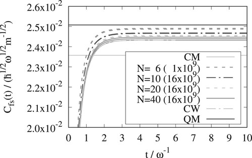
Figure 2. As in Figure 1 but for the x-version of OPCW.

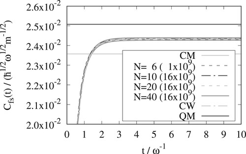
Figure 3. As in Figure 1 but for $\text{β}\hslash \omega =3$.

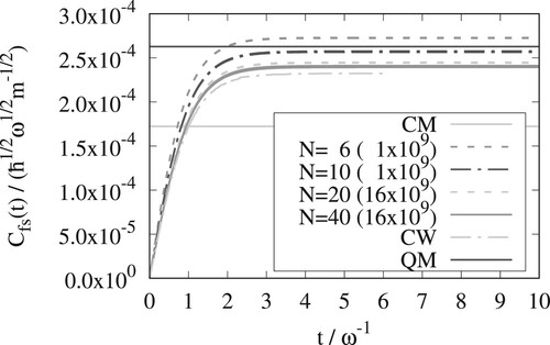
Figure 4. As in Figure 1 but for $\text{β}\hslash \omega =3$ and the x-version of OPCW.

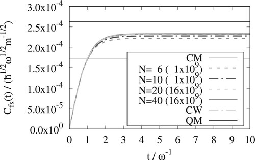
Figure 5. As in figure 1 but for $\text{β}\hslash \omega =6$.

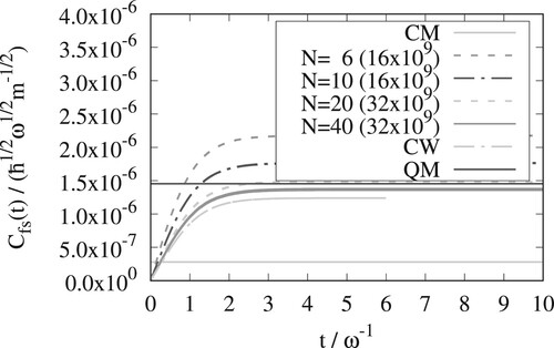
Figure 6. As in figure 1 but for $\text{β}\hslash \omega =6$ and the x-version of OPCW.

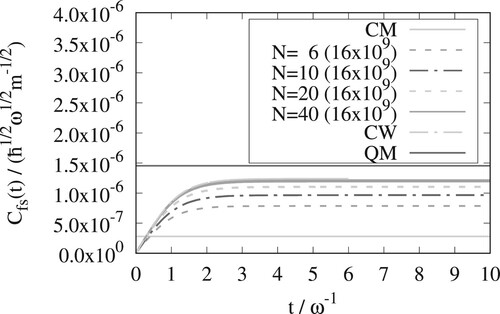
Figure 7. As in figure 1 but for $\text{β}\hslash \omega =12$ and the x-version of OPCW.

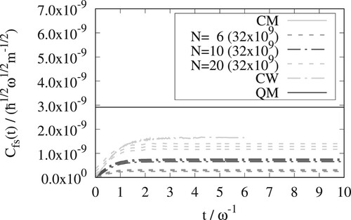
Table 1. Rate constants ($k_{\text{r}}$) for different inverse temperatures (β) for the Eckart barrier described in Equation 24(24) $V_{\text{Eckart}}\left(x\right)=\frac{6\hslash \omega }{\pi }{\mathrm{s}\mathrm{e}\mathrm{c}\mathrm{h}}^2\left(\sqrt{\frac{\pi m\omega }{12\hslash }}x\right),$(24) . Comparision of OPCW[x-version, N = 40], Ring Polymer Molecular Dynamics (RPMD), classical mechanics (CM), exact Classical Wigner (CW), and quantum mechanics (QM). Note that for $\text{β}=12$ only N = 20 was used for OPCW.

	$k_{\text{r}}/\left({\hslash }^{\frac{1}{2}}{\omega }^{\frac{1}{2}}{m}^{-\frac{1}{2}}\right)$
$\text{β}\hslash \omega$	OPCW	RPMD	CM	CW	QM
1	$6.10\times {10}^{-2}$	$6.17\times {10}^{-2}$	$5.9084\times {10}^{-2}$	$6.10\times {10}^{-2}$	$6.2856\times {10}^{-2}$
3	1.01 $\times {10}^{-3}$	1.07 $\times {10}^{-3}$	7.4821 $\times {10}^{-4}$	1.01 $\times {10}^{-3}$	1.1409 $\times {10}^{-3}$
6	7.39 $\times {10}^{-6}$	7.46 $\times {10}^{-6}$	1.7186 $\times {10}^{-6}$	7.61 $\times {10}^{-6}$	8.9347 $\times {10}^{-6}$
12	$1.\times {10}^{-8}$	1.39 $\times {10}^{-8}$	1.2824 $\times {10}^{-11}$	1.4 $\times {10}^{-8}$	2.5306 $\times {10}^{-8}$

Table 2. Tunneling factors (Γ) for different inverse temperatures (β) for the Eckart barrier described in Equation 24(24) $V_{\text{Eckart}}\left(x\right)=\frac{6\hslash \omega }{\pi }{\mathrm{s}\mathrm{e}\mathrm{c}\mathrm{h}}^2\left(\sqrt{\frac{\pi m\omega }{12\hslash }}x\right),$(24) . Comparision of OPCW[x-version, N = 40], Ring Polymer Molecular Dynamics (RPMD), exact Classical Wigner (CW), and exact results. Note that for $\text{β}=12$ only N = 20 was used for OPCW.

$\text{β}\hslash \omega$	${\mathrm{\Gamma }}_{\text{OPCW}}$	${\mathrm{\Gamma }}_{\text{RPMD}}$	${\mathrm{\Gamma }}_{\text{CW}}$	${\mathrm{\Gamma }}_{\text{Exact}}$
1	1.03	1.04	1.03	1.0638
3	1.35	1.43	1.35	1.5249
6	4.30	4.34	4.43	5.1987
12	9. $\times {10}^2$	1.09 $\times {10}^3$	1.1 $\times {10}^3$	1973.3

At $\text{β}\hslash \omega =1$ the quantum mechanical rate constant is only $\sim 6\mathrm{\%}$ bigger than the classical one. For the three lower temperatures the differences are significantly bigger, i.e. the quantum mechanical rate constant is $\sim 50\mathrm{\%}$ bigger for $\text{β}\hslash \omega =3$, a factor $\sim 5$ bigger for $\text{β}\hslash \omega =6$ and finally a factor of $\sim 2000$ bigger at the lowest temperature. The classical Wigner method gives rate constants that are intermediate between classical mechanics and quantum mechanics, but for the three lower temperatures they represent a significant improvement over the classical result.

The OPCW results converge to the exact classical Wigner result as the number of beads is increased. From Figures 1–6 it can be seen that the y-version of the OPCW method needs more beads than the x-version. The x-version of the OPCW method has excellent convergence with respect to the number of beads. $C_{\text{fs},y}\left(t\right)$ converge from above and $C_{\text{fs},x}\left(t\right)$ converge from below. Both the x and y versions of OPCW give results that are close to the exact classical Wigner result.

The RPMD and classical Wigner methods give similar results for all temperatures. Results from a single, symmetric, one-dimensional, potential is, however, not enough to draw general conclusions.

7. Conclusion and outlook

In this work, the recently developed Open Polymer Classical Wigner (OPCW) method [13] is extended to the flux-Heaviside trace of Miller [15] and applied to a symmetric Eckart potential, for four temperatures. For all but the lowest temperature, the OPCW method can be converged to the exact classical Wigner result by increasing the number of beads in the path integral polymer. For the lowest temperature, a strict convergence of the OPCW result was computationally too demanding, but a result some thirty percent from the exact Classical Wigner model was obtained, see Figure 7. This should be compared to the classical prediction that is about two thousand times smaller than exact quantum mechanics. Particularly the x-version of the OPCW method shows promise for further tests.

In the future, it would be of interest to apply the OPCW model to reaction rate constant calculations of multidimensional systems, such as the double well potential of Topaler and Makri [29] coupled to the harmonic bath of Caldeira and Leggett [30]. For such a system it could be beneficial to modify the OPCW calculations by making the bath classical, as illustrated in the preceding article [13]. There a ten-dimensional problem was considered. A more elaborate approach would be to keep an intermediate number of beads for the bath degrees of freedom, while still retaining the full number for the reaction coordinate. Such an approach will be the subject of future research. It would also be of interest to try the method on asymmetric potentials. Such potentials are challenging not just for the OPCW method but for all classical Wigner implementations, since the positioning of the dividing surface is not obvious. However, Liu and Miller have shown that this can be done successfully [4].

For systems where the reactants are bound it could be of interest to use the Heaviside-Heaviside trace of Miller et al. [14] instead of the flux-Heaviside trace.

Acknowledgments

Financial support from the Swedish Research Council (Vetenskapsrådet), diary numbers 2016-03275 and 2020-05293, is acknowledged. The computations in this work were performed at Chalmers Centre for Computational Science and Engineering (C3SE), a partner center of the Swedish National Infrastructure for Computing (SNIC).

Disclosure statement

No potential conflict of interest was reported by the author(s).

Additional information

Funding

Swedish Research Council 2020-05293; Swedish Research Council 2016-03275

Appendices

1

To obtain an expression corresponding to the $x_1$-version of OPCW we start from equation 8(8) $\begin{array}{rl}{C}_{\text{fs}}\left(t\right)& =\left\{\prod _{j=1}^N{\int }_{-\mathrm{\infty }}^{\mathrm{\infty }}\text{d}{x}_j\right\}〈x_1\left|{\text{e}}^{-\frac{\text{β}}{N}\hat{H}}\right|x_2〉〈x_2\left|{\text{e}}^{-\frac{\text{β}}{N}\hat{H}}\right|x_3〉\\ & \dots 〈x_{\frac{N}{2}}\left|{\text{e}}^{-\frac{\text{β}}{N}\hat{H}}\hat{F}\right|x_{\frac{N}{2}+1}〉\\ & \dots 〈x_{N-1}\left|{\text{e}}^{-\frac{\text{β}}{N}\hat{H}}\right|x_N〉\\ & \times 〈x_N\left|{\text{e}}^{-\frac{\text{β}}{N}\hat{H}}{\text{e}}^{\frac{\mathrm{i}\hat{H}t}{\hslash }}h\left(\hat{x}\right){\text{e}}^{-\frac{\mathrm{i}\hat{H}t}{\hslash }}\right|x_1〉\end{array}$(8) . There the $\hat{x}$-dependent parts of $\hat{F}$ have to operate to the right in the matrix element before rewriting as Wigner transforms. To be able to operate to the right, the flux operator has to be rearranged into a form where all $\hat{x}$-dependence is to the right of all $\hat{p}$-dependence. Using that $\hat{p}=-\mathrm{i}\hslash \frac{\text{d}}{\text{d}x}$ this can be achieved as (A1) $\begin{array}{rl}\hat{F}& =\frac{1}{2m}\left(\delta \left(\hat{x}\right)\hat{p}+\hat{p}\delta \left(\hat{x}\right)\right)=\frac{1}{2m}\left(\left[\delta \left(\hat{x}\right),\hat{p}\right]+\hat{p}\delta \left(\hat{x}\right)+\hat{p}\delta \left(\hat{x}\right)\right)\\ & =\frac{1}{2m}\left(-\mathrm{i}\hslash \left(\delta \left(\hat{x}\right)\frac{\text{d}}{\text{d}x}-\frac{\text{d}}{\text{d}x}\delta \left(\hat{x}\right)\right)+2\hat{p}\delta \left(\hat{x}\right)\right)\\ & =\frac{1}{2m}\left(-\mathrm{i}\hslash \left(\delta \left(\hat{x}\right)\frac{\text{d}}{\text{d}x}-\frac{\text{d}\delta \left(\hat{x}\right)}{\text{d}x}-\delta \left(\hat{x}\right)\frac{\text{d}}{\text{d}x}\right)+2\hat{p}\delta \left(\hat{x}\right)\right)\\ & =\frac{1}{2m}\left(\mathrm{i}\hslash \frac{\text{d}\delta \left(\hat{x}\right)}{\text{d}x}+2\hat{p}\delta \left(\hat{x}\right)\right),\end{array}$(A1) where the square brackets denote a commutator. Using this new form of the flux operator and operating $\hat{x}$ to the right we obtain (A2) $\begin{array}{rl}{C}_{\text{fs}}\left(t\right)& =\left\{\prod _{j=1}^N{\int }_{-\mathrm{\infty }}^{\mathrm{\infty }}\text{d}{x}_j\right\}〈x_1\left|{\text{e}}^{-\frac{\text{β}}{N}\hat{H}}\right|x_2〉〈x_2\left|{\text{e}}^{-\frac{\text{β}}{N}\hat{H}}\right|x_3〉\\ & \dots \left(〈x_{\frac{N}{2}}\left|{\text{e}}^{-\frac{\text{β}}{N}\hat{H}}\hat{p}\right|x_{\frac{N}{2}+1}〉\frac{1}{m}\delta \left(x_{\frac{N}{2}+1}\right)\phantom{\frac{\text{d}\delta \left(x_{\frac{N}{2}+1}\right)}{\text{d}{x}_{\frac{N}{2}+1}}}\right.\\ & \left.+〈x_{\frac{N}{2}}\left|{\text{e}}^{-\frac{\text{β}}{N}\hat{H}}\right|x_{\frac{N}{2}+1}〉\frac{\mathrm{i}\hslash }{2m}\frac{\text{d}\delta \left(x_{\frac{N}{2}+1}\right)}{\text{d}{x}_{\frac{N}{2}+1}}\right)\\ & \dots 〈x_{N-1}\left|{\text{e}}^{-\frac{\text{β}}{N}\hat{H}}\right|x_N〉〈x_N\left|{\text{e}}^{-\frac{\text{β}}{N}\hat{H}}{\text{e}}^{\frac{\mathrm{i}\hat{H}t}{\hslash }}h\left(\hat{x}\right){\text{e}}^{-\frac{\mathrm{i}\hat{H}t}{\hslash }}\right|x_1〉.\end{array}$(A2) Rewriting as Wigner transforms, taking the limit where the Wigner transform of the Boltzmann operator is the classical Boltzmann factor, and assuming that $V\left(y_j\right)$ is independent of momentum, a new way to write Equation 11(11) $\begin{array}{rl}{C}_{\text{fs}}\left(t\right)& =\underset{N\to \mathrm{\infty }}{lim}{\left(\frac{mN}{2\pi \text{β}}\right)}^{\frac{N}{2}}\frac{\text{β}}{2\pi mN}{\hslash }^{-N}\left\{\prod _{j=1}^N{\int }_{-\mathrm{\infty }}^{\mathrm{\infty }}\text{d}{x}_j\right\}\\ & \times {\iint }_{-\mathrm{\infty }}^{\mathrm{\infty }}\text{d}{p}_{\frac{N}{2}}\text{d}{p}_N{\text{e}}^{-\frac{\text{β}}{N}\sum _{j=1}^{N}V\left(y_j\right)}\\ & \times {\text{e}}^{-\frac{mN}{2{\hslash }^2\text{β}}\left(\sum _{j=1}^{\frac{N}{2}-1}{\left(x_{j+1}-x_j\right)}^2+\sum _{j=\frac{N}{2}+1}^{N-1}{\left(x_{j+1}-x_j\right)}^2\right)}\\ & \times {\text{e}}^{-\frac{\mathrm{i}}{\hslash }{p}_{\frac{N}{2}}\left(x_{\frac{N}{2}+1}-x_{\frac{N}{2}}\right)}{\text{e}}^{-\frac{\text{β}}{N}\frac{p_{\frac{N}{2}}^2}{2m}}{\left(\hat{F}\right)}_{\text{W}}\left[y_{\frac{N}{2}},p_{\frac{N}{2}}\right]\\ & \times {\text{e}}^{-\frac{\mathrm{i}}{\hslash }{p}_N\left(x_1-x_N\right)}{\text{e}}^{-\frac{\text{β}}{N}\frac{p_N^2}{2m}}\\ & \times {\left({\text{e}}^{\frac{\mathrm{i}\hat{H}t}{\hslash }}h\left(\hat{x}\right){\text{e}}^{-\frac{\mathrm{i}\hat{H}t}{\hslash }}\right)}_{\text{W}}\left[y_N,p_N\right],\end{array}$(11) can be obtained: (A3) $\begin{array}{rl}{C}_{\text{fs}}\left(t\right)& =\underset{N\to \mathrm{\infty }}{lim}{\left(\frac{mN}{2\pi \text{β}}\right)}^{\frac{N}{2}}\frac{\text{β}}{2\pi mN}{\hslash }^{-N}\left\{\prod _{j=1}^N{\int }_{-\mathrm{\infty }}^{\mathrm{\infty }}\text{d}{x}_j\right\}\\ & \times {\iint }_{-\mathrm{\infty }}^{\mathrm{\infty }}\text{d}{p}_{\frac{N}{2}}\text{d}{p}_N{\text{e}}^{-\frac{\text{β}}{N}\sum _{j=1}^{N}V\left(y_j\right)}\\ & \times {\text{e}}^{-\frac{mN}{2{\hslash }^2\text{β}}\left(\sum _{j=1}^{\frac{N}{2}-1}{\left(x_{j+1}-x_j\right)}^2+\sum _{j=\frac{N}{2}+1}^{N-1}{\left(x_{j+1}-x_j\right)}^2\right)}\\ & \times {\text{e}}^{-\frac{\mathrm{i}}{\hslash }{p}_{\frac{N}{2}}\left(x_{\frac{N}{2}+1}-x_{\frac{N}{2}}\right)}{\text{e}}^{-\frac{\text{β}}{N}\frac{p_{\frac{N}{2}}^2}{2m}}\\ & \times \left({\left(\hat{p}\right)}_{\text{W}}\left[y_{\frac{N}{2}},p_{\frac{N}{2}}\right]\frac{1}{m}\delta \left(x_{\frac{N}{2}+1}\right)+\frac{\mathrm{i}\hslash }{2m}\frac{\text{d}\delta \left(x_{\frac{N}{2}+1}\right)}{\text{d}{x}_{\frac{N}{2}+1}}\right)\\ & \times {\text{e}}^{-\frac{\mathrm{i}}{\hslash }{p}_N\left(x_1-x_N\right)}{\text{e}}^{-\frac{\text{β}}{N}\frac{p_N^2}{2m}}{\left({\text{e}}^{\frac{\mathrm{i}\hat{H}t}{\hslash }}h\left(\hat{x}\right){\text{e}}^{-\frac{\mathrm{i}\hat{H}t}{\hslash }}\right)}_{\text{W}}\left[y_N,p_N\right].\end{array}$(A3)

Knowing that ${\left(\hat{p}\right)}_{\text{W}}\left[x,p\right]=p$, $p_{\frac{N}{2}}$ can be integrated out as (A4) $\begin{array}{rl}& \frac{{\int }_{-\mathrm{\infty }}^{\mathrm{\infty }}\text{d}{p}_{\frac{N}{2}}{\left(\hat{p}\right)}_{\text{W}}\left[y_{\frac{N}{2}},p_{\frac{N}{2}}\right]{\text{e}}^{-\frac{\text{β}}{N}\frac{p_{\frac{N}{2}}^2}{2m}}{\text{e}}^{-\frac{\mathrm{i}}{\hslash }{p}_{\frac{N}{2}}\left(x_{\frac{N}{2}+1}-x_{\frac{N}{2}}\right)}}{{\int }_{-\mathrm{\infty }}^{\mathrm{\infty }}\text{d}{p}_{\frac{N}{2}}{\text{e}}^{-\frac{\text{β}}{N}\frac{p_{\frac{N}{2}}^2}{2m}}{\text{e}}^{-\frac{\mathrm{i}}{\hslash }{p}_{\frac{N}{2}}\left(x_{\frac{N}{2}+1}-x_{\frac{N}{2}}\right)}}\\ & =\frac{{\int }_{-\mathrm{\infty }}^{\mathrm{\infty }}\text{d}{p}_{\frac{N}{2}}{p}_{\frac{N}{2}}{\text{e}}^{-\frac{\text{β}}{N}\frac{p_{\frac{N}{2}}^2}{2m}}{\text{e}}^{-\frac{\mathrm{i}}{\hslash }{p}_{\frac{N}{2}}\left(x_{\frac{N}{2}+1}-x_{\frac{N}{2}}\right)}}{\sqrt{\frac{2\pi mN}{\text{β}}}{\text{e}}^{-\frac{\text{β}}{N}\frac{m{N}^2{\left(x_{\frac{N}{2}+1}-x_{\frac{N}{2}}\right)}^2}{2{\hslash }^2{\text{β}}^2}}}\\ & =-\frac{\mathrm{i}Nm}{\hslash \text{β}}\left(x_{\frac{N}{2}+1}-x_{\frac{N}{2}}\right)\end{array}$(A4) and we get (A5) $\begin{array}{rl}{C}_{\text{fs}}\left(t\right)& =\underset{N\to \mathrm{\infty }}{lim}{\left(\frac{mN}{2\pi \text{β}}\right)}^{\frac{N}{2}}\sqrt{\frac{\text{β}}{2\pi mN}}{\hslash }^{-N}\\ & \times \left\{\prod _{j=1}^N{\int }_{-\mathrm{\infty }}^{\mathrm{\infty }}\text{d}{x}_j\right\}{\int }_{-\mathrm{\infty }}^{\mathrm{\infty }}\text{d}{p}_N{\text{e}}^{-\frac{\text{β}}{N}\sum _{j=1}^{N}V\left(y_j\right)}\\ & \times {\text{e}}^{-\frac{mN}{2{\hslash }^2\text{β}}\sum _{j=1}^{N-1}{\left(x_{j+1}-x_j\right)}^2}\\ & \times \left(\phantom{\frac{\text{β}{z}^{\text{β}}{N}_{\gamma ,k}\left({\mu }_{k}z\right)}{{\mu }_k^2}}-\frac{\mathrm{i}N}{\hslash \text{β}}\left(x_{\frac{N}{2}+1}-x_{\frac{N}{2}}\right)\delta \left(x_{\frac{N}{2}+1}\right)\phantom{\frac{\text{d}\delta \left(x_{\frac{N}{2}+1}\right)}{\text{d}{x}_{\frac{N}{2}+1}}}\right.\\ & +\left.\frac{\mathrm{i}\hslash }{2m}\frac{\text{d}\delta \left(x_{\frac{N}{2}+1}\right)}{\text{d}{x}_{\frac{N}{2}+1}}\right){\text{e}}^{-\frac{\mathrm{i}}{\hslash }{p}_N\left(x_1-x_N\right)}\\ & \times {\text{e}}^{-\frac{\text{β}}{N}\frac{p_N^2}{2m}}{\left({\text{e}}^{\frac{\mathrm{i}\hat{H}t}{\hslash }}h\left(\hat{x}\right){\text{e}}^{-\frac{\mathrm{i}\hat{H}t}{\hslash }}\right)}_{\text{W}}\left[y_N,p_N\right].\end{array}$(A5) If $f\left(x\right)$ is a function of x then ${\int }_{-\mathrm{\infty }}^{\mathrm{\infty }}\text{d}xf\left(x\right)\frac{\text{d}\delta \left(x\right)}{\text{d}x}={\int }_{-\mathrm{\infty }}^{\mathrm{\infty }}\text{d}x(-\frac{\text{d}f\left(x\right)}{\text{d}x})\delta \left(x\right)$. This can be used to eliminate the derivative of the delta function through (A6) $\begin{array}{rl}& {\int }_{-\mathrm{\infty }}^{\mathrm{\infty }}\text{d}{x}_{\frac{N}{2}+1}{\text{e}}^{-\frac{\text{β}}{N}\left(V\left(y_{\frac{N}{2}}\right)+V\left(y_{\frac{N}{2}+1}\right)\right)}\\ & \times {\text{e}}^{-\frac{mN}{2{\hslash }^2\text{β}}\left({\left(x_{\frac{N}{2}+1}-x_{\frac{N}{2}}\right)}^2+{\left(x_{\frac{N}{2}+2}-x_{\frac{N}{2}+1}\right)}^2\right)}\frac{\mathrm{i}\hslash }{2m}\frac{\text{d}\delta \left(x_{\frac{N}{2}+1}\right)}{\text{d}{x}_{\frac{N}{2}+1}}\\ & ={\int }_{-\mathrm{\infty }}^{\mathrm{\infty }}\text{d}{x}_{\frac{N}{2}+1}{\text{e}}^{-\frac{\text{β}}{N}\left(V\left(y_{\frac{N}{2}}\right)+V\left(y_{\frac{N}{2}+1}\right)\right)}\\ & \times {\text{e}}^{-\frac{mN}{2{\hslash }^2\text{β}}\left({\left(x_{\frac{N}{2}+1}-x_{\frac{N}{2}}\right)}^2+{\left(x_{\frac{N}{2}+2}-x_{\frac{N}{2}+1}\right)}^2\right)}\frac{\mathrm{i}\hslash }{2m}\delta \left(x_{\frac{N}{2}+1}\right)\\ & \times (-1)\left(-\frac{\text{β}}{N}\left(\frac{1}{2}\frac{\text{d}V\left(y_{\frac{N}{2}}\right)}{\text{d}{y}_{\frac{N}{2}}}+\frac{1}{2}\frac{\text{d}V\left(y_{\frac{N}{2}+1}\right)}{\text{d}{y}_{\frac{N}{2}+1}}\right)\right.\\ & -\left.\phantom{\frac{\text{d}V\left(y_{\frac{N}{2}+1}\right)}{\text{d}{y}_{\frac{N}{2}+1}}\frac{\text{β}{z}^{\text{β}}{N}_{\gamma ,k}\left({\mu }_{k}z\right)}{{\mu }_k^2}}\frac{mN}{2{\hslash }^2\text{β}}\left(2\left(x_{\frac{N}{2}+1}-x_{\frac{N}{2}}\right)-2\left(x_{\frac{N}{2}+2}-x_{\frac{N}{2}+1}\right)\right)\right)\\ & ={\int }_{-\mathrm{\infty }}^{\mathrm{\infty }}\text{d}{x}_{\frac{N}{2}+1}{\text{e}}^{-\frac{\text{β}}{N}\left(V\left(y_{\frac{N}{2}}\right)+V\left(y_{\frac{N}{2}+1}\right)\right)}\\ & \times {\text{e}}^{-\frac{mN}{2{\hslash }^2\text{β}}\left({\left(x_{\frac{N}{2}+1}-x_{\frac{N}{2}}\right)}^2+{\left(x_{\frac{N}{2}+2}-x_{\frac{N}{2}+1}\right)}^2\right)}\\ & \times \left(\frac{i\hslash \text{β}}{4Nm}\left(\frac{\text{d}V\left(y_{\frac{N}{2}}\right)}{\text{d}{y}_{\frac{N}{2}}}+\frac{\text{d}V\left(y_{\frac{N}{2}+1}\right)}{\text{d}{y}_{\frac{N}{2}+1}}\right)\right.\\ & +\left.\phantom{\frac{\text{d}V\left(y_{\frac{N}{2}+1}\right)}{\text{d}{y}_{\frac{N}{2}+1}}\frac{\text{β}{z}^{\text{β}}{N}_{\gamma ,k}\left({\mu }_{k}z\right)}{{\mu }_k^2}}\frac{\mathrm{i}N}{2\hslash \text{β}}\left(2x_{\frac{N}{2}+1}-x_{\frac{N}{2}}-x_{\frac{N}{2}+2}\right)\right)\delta \left(x_{\frac{N}{2}+1}\right),\end{array}$(A6) leading to (A7) $\begin{array}{rl}{C}_{\text{fs}}\left(t\right)& =\underset{N\to \mathrm{\infty }}{lim}{\left(\frac{mN}{2\pi \text{β}}\right)}^{\frac{N}{2}}\sqrt{\frac{\text{β}}{2\pi mN}}{\hslash }^{-N}\left\{\prod _{j=1}^N{\int }_{-\mathrm{\infty }}^{\mathrm{\infty }}\text{d}{x}_j\right\}\\ & \times {\int }_{-\mathrm{\infty }}^{\mathrm{\infty }}\text{d}{p}_N{\text{e}}^{-\frac{\text{β}}{N}\sum _{j=1}^{N}V\left(y_j\right)}{\text{e}}^{-\frac{mN}{2{\hslash }^2\text{β}}\sum _{j=1}^{N-1}{\left(x_{j+1}-x_j\right)}^2}\\ & \times \left(-\frac{\mathrm{i}N}{\hslash \text{β}}\left(x_{\frac{N}{2}+1}-x_{\frac{N}{2}}\right)\delta \left(x_{\frac{N}{2}+1}\right)\phantom{\frac{\text{d}V\left(y_{\frac{N}{2}-1}\right)}{\text{d}{x}_{\frac{N}{2}+1}}}\right.\\ & +\left(\frac{\mathrm{i}\hslash \text{β}}{4Nm}\left(\frac{\text{d}V\left(y_{\frac{N}{2}}\right)}{\text{d}{y}_{\frac{N}{2}}}+\frac{\text{d}V\left(y_{\frac{N}{2}+1}\right)}{\text{d}{y}_{\frac{N}{2}+1}}\right)\right.\\ & \left.+\left.\phantom{\frac{\text{d}V\left(y_{\frac{N}{2}+1}\right)}{\text{d}{y}_{\frac{N}{2}+1}}}\frac{\mathrm{i}N}{2\hslash \text{β}}\left(2x_{\frac{N}{2}+1}-x_{\frac{N}{2}}-x_{\frac{N}{2}+2}\right)\right)\delta \left(x_{\frac{N}{2}+1}\right)\phantom{\frac{\text{β}{z}^{\text{β}}{N}_{\gamma ,k}\left({\mu }_{k}z\right)}{{\mu }_k^2}}\right)\\ & \times {\text{e}}^{-\frac{\mathrm{i}}{\hslash }{p}_N\left(x_1-x_N\right)}{\text{e}}^{-\frac{\text{β}}{N}\frac{p_N^2}{2m}}{\left({\text{e}}^{\frac{\mathrm{i}\hat{H}t}{\hslash }}h\left(\hat{x}\right){\text{e}}^{-\frac{\mathrm{i}\hat{H}t}{\hslash }}\right)}_{\text{W}}\left[y_N,p_N\right]\\ & =\underset{N\to \mathrm{\infty }}{lim}{\left(\frac{mN}{2\pi \text{β}}\right)}^{\frac{N}{2}}\sqrt{\frac{\text{β}}{2\pi mN}}{\hslash }^{-N}\left\{\prod _{j=1}^N{\int }_{-\mathrm{\infty }}^{\mathrm{\infty }}\text{d}{x}_j\right\}\\ & \times {\int }_{-\mathrm{\infty }}^{\mathrm{\infty }}\text{d}{p}_N{\text{e}}^{-\frac{\text{β}}{N}\sum _{j=1}^{N}V\left(y_j\right)}{\text{e}}^{-\frac{mN}{2{\hslash }^2\text{β}}\sum _{j=1}^{N-1}{\left(x_{j+1}-x_j\right)}^2}\\ & \times \left(\frac{\mathrm{i}\hslash \text{β}}{4Nm}\left(\frac{\text{d}V\left(y_{\frac{N}{2}}\right)}{\text{d}{y}_{\frac{N}{2}}}+\frac{\text{d}V\left(y_{\frac{N}{2}+1}\right)}{\text{d}{y}_{\frac{N}{2}+1}}\right)\right.\\ & +\left.\phantom{\frac{\text{d}V\left(y_{\frac{N}{2}+1}\right)}{\text{d}{y}_{\frac{N}{2}+1}}}\frac{\mathrm{i}N}{2\hslash \text{β}}\left(2x_{\frac{N}{2}+1}-x_{\frac{N}{2}}-x_{\frac{N}{2}+2}-2x_{\frac{N}{2}+1}+2x_{\frac{N}{2}}\right)\phantom{\frac{\text{β}{z}^{\text{β}}{N}_{\gamma ,k}\left({\mu }_{k}z\right)}{{\mu }_k^2}}\right)\\ & \times \delta \left(x_{\frac{N}{2}+1}\right){\text{e}}^{-\frac{\mathrm{i}}{\hslash }{p}_N\left(x_1-x_N\right)}\\ & \times {\text{e}}^{-\frac{\text{β}}{N}\frac{p_N^2}{2m}}{\left({\text{e}}^{\frac{\mathrm{i}\hat{H}t}{\hslash }}h\left(\hat{x}\right){\text{e}}^{-\frac{\mathrm{i}\hat{H}t}{\hslash }}\right)}_{\text{W}}\left[y_N,p_N\right]\\ & =\underset{N\to \mathrm{\infty }}{lim}{\left(\frac{mN}{2\pi \text{β}}\right)}^{\frac{N}{2}}\sqrt{\frac{\text{β}}{2\pi mN}}{\hslash }^{-N}\left\{\prod _{j=1}^N{\int }_{-\mathrm{\infty }}^{\mathrm{\infty }}\text{d}{x}_j\right\}\\ & \times {\int }_{-\mathrm{\infty }}^{\mathrm{\infty }}\text{d}{p}_N{\text{e}}^{-\frac{\text{β}}{N}\sum _{j=1}^{N}V\left(y_j\right)}{\text{e}}^{-\frac{mN}{2{\hslash }^2\text{β}}\sum _{j=1}^{N-1}{\left(x_{j+1}-x_j\right)}^2}\\ & \times \left(\frac{\mathrm{i}\hslash \text{β}}{4Nm}\left(\frac{\text{d}V\left(y_{\frac{N}{2}}\right)}{\text{d}{y}_{\frac{N}{2}}}+\frac{\text{d}V\left(y_{\frac{N}{2}+1}\right)}{\text{d}{y}_{\frac{N}{2}+1}}\right)\right.\\ & +\left.\phantom{\frac{\text{d}V\left(y_{\frac{N}{2}+1}\right)}{\text{d}{y}_{\frac{N}{2}+1}}}\frac{\mathrm{i}N}{2\hslash \text{β}}\left(x_{\frac{N}{2}}-x_{\frac{N}{2}+2}\right)\phantom{\frac{\text{β}{z}^{\text{β}}{N}_{\gamma ,k}\left({\mu }_{k}z\right)}{{\mu }_k^2}}\right)\delta \left(x_{\frac{N}{2}+1}\right)\\ & \times {\text{e}}^{-\frac{\mathrm{i}}{\hslash }{p}_N\left(x_1-x_N\right)}{\text{e}}^{-\frac{\text{β}}{N}\frac{p_N^2}{2m}}\\ & \times {\left({\text{e}}^{\frac{\mathrm{i}\hat{H}t}{\hslash }}h\left(\hat{x}\right){\text{e}}^{-\frac{\mathrm{i}\hat{H}t}{\hslash }}\right)}_{\text{W}}\left[y_N,p_N\right].\end{array}$(A7) Up to this point the new derivation is equivalent to what was done for the y-version up to Equation 14(14) $\begin{array}{rl}{C}_{\text{fs}}\left(t\right)& =\underset{N\to \mathrm{\infty }}{lim}{\left(\frac{mN}{2\pi \text{β}}\right)}^{\frac{N}{2}}\sqrt{\frac{\text{β}}{2\pi mN}}{\hslash }^{-N}\left\{\prod _{j=1}^N{\int }_{-\mathrm{\infty }}^{\mathrm{\infty }}\text{d}{x}_j\right\}\\ & \times {\int }_{-\mathrm{\infty }}^{\mathrm{\infty }}\text{d}{p}_N{\text{e}}^{-\frac{\text{β}}{N}\sum _{j=1}^{N}V\left(y_j\right)}\\ & \times {\text{e}}^{-\frac{mN}{2{\hslash }^2\text{β}}\sum _{j=1}^{N-1}{\left(x_{j+1}-x_j\right)}^2}\\ & \times \frac{\mathrm{i}N}{\hslash \text{β}}\left(x_{\frac{N}{2}}-x_{\frac{N}{2}+1}\right)\delta \left(y_{\frac{N}{2}}\right)\\ & \times {\text{e}}^{-\frac{\mathrm{i}}{\hslash }{p}_N\left(x_1-x_N\right)}{\text{e}}^{-\frac{\text{β}}{N}\frac{p_N^2}{2m}}\\ & \times {\left({\text{e}}^{\frac{\mathrm{i}\hat{H}t}{\hslash }}h\left(\hat{x}\right){\text{e}}^{-\frac{\mathrm{i}\hat{H}t}{\hslash }}\right)}_{\text{W}}\left[y_N,p_N\right].\end{array}$(14) . However, once this expression is subjected to the classical Wigner approximation and by assuming finite N, this is not the case anymore, as we obtain (A8) $\begin{array}{rl}{C}_{\text{fs},x}\left(t\right)& \approx {\left(\frac{mN}{2\pi \text{β}}\right)}^{\frac{N}{2}}\sqrt{\frac{\text{β}}{2\pi mN}}{\hslash }^{-N}\\ & \times \left\{\prod _{j=1}^N{\int }_{-\mathrm{\infty }}^{\mathrm{\infty }}\text{d}{x}_j\right\}{\int }_{-\mathrm{\infty }}^{\mathrm{\infty }}\text{d}{p}_N{\text{e}}^{-\frac{\mathrm{i}}{\hslash }{p}_N\left(x_1-x_N\right)}\\ & \times {\text{e}}^{-\frac{\text{β}}{N}\left(\frac{p_N^2}{2m}+\sum _{j=1}^{N}V\left(y_j\right)+\frac{m{N}^2}{2{\hslash }^2{\text{β}}^2}\sum _{j=1}^{N-1}{\left(x_{j+1}-x_j\right)}^2\right)}\\ & \times \left(\frac{\mathrm{i}\hslash \text{β}}{4Nm}\left(\frac{\text{d}V\left(y_{\frac{N}{2}}\right)}{\text{d}{y}_{\frac{N}{2}}}+\frac{\text{d}V\left(y_{\frac{N}{2}+1}\right)}{\text{d}{y}_{\frac{N}{2}+1}}\right)\right.\\ & +\left.\phantom{\frac{\text{d}V\left(y_{\frac{N}{2}+1}\right)}{\text{d}{y}_{\frac{N}{2}+1}}}\frac{\mathrm{i}N}{2\hslash \text{β}}\left(x_{\frac{N}{2}}-x_{\frac{N}{2}+2}\right)\phantom{\frac{\text{β}{z}^{\text{β}}{N}_{\gamma ,k}\left({\mu }_{k}z\right)}{{\mu }_k^2}}\right)\delta \left(x_{\frac{N}{2}+1}\right)\\ & \times h\left(x\left(y_N,p_N,t\right)\right).\end{array}$(A8) Equation A8(A8) $\begin{array}{rl}{C}_{\text{fs},x}\left(t\right)& \approx {\left(\frac{mN}{2\pi \text{β}}\right)}^{\frac{N}{2}}\sqrt{\frac{\text{β}}{2\pi mN}}{\hslash }^{-N}\\ & \times \left\{\prod _{j=1}^N{\int }_{-\mathrm{\infty }}^{\mathrm{\infty }}\text{d}{x}_j\right\}{\int }_{-\mathrm{\infty }}^{\mathrm{\infty }}\text{d}{p}_N{\text{e}}^{-\frac{\mathrm{i}}{\hslash }{p}_N\left(x_1-x_N\right)}\\ & \times {\text{e}}^{-\frac{\text{β}}{N}\left(\frac{p_N^2}{2m}+\sum _{j=1}^{N}V\left(y_j\right)+\frac{m{N}^2}{2{\hslash }^2{\text{β}}^2}\sum _{j=1}^{N-1}{\left(x_{j+1}-x_j\right)}^2\right)}\\ & \times \left(\frac{\mathrm{i}\hslash \text{β}}{4Nm}\left(\frac{\text{d}V\left(y_{\frac{N}{2}}\right)}{\text{d}{y}_{\frac{N}{2}}}+\frac{\text{d}V\left(y_{\frac{N}{2}+1}\right)}{\text{d}{y}_{\frac{N}{2}+1}}\right)\right.\\ & +\left.\phantom{\frac{\text{d}V\left(y_{\frac{N}{2}+1}\right)}{\text{d}{y}_{\frac{N}{2}+1}}}\frac{\mathrm{i}N}{2\hslash \text{β}}\left(x_{\frac{N}{2}}-x_{\frac{N}{2}+2}\right)\phantom{\frac{\text{β}{z}^{\text{β}}{N}_{\gamma ,k}\left({\mu }_{k}z\right)}{{\mu }_k^2}}\right)\delta \left(x_{\frac{N}{2}+1}\right)\\ & \times h\left(x\left(y_N,p_N,t\right)\right).\end{array}$(A8) is the expression corresponding to the $x_1$-version of OPCW for the flux-Heaviside trace. Due to the symmetrisation of the trace $x_{\frac{N}{2}+1}$ rather than $x_1$ is used. This trace is called $C_{\text{fs},x}\left(t\right)$ in the main text.

2

Here we show how to calculate the $Z_{\delta }$ factor using a Monte-Carlo implementation of the effective frequency theory of Feynman and Kleinert (FK). For an introduction to the FK theory, we refer the reader to Hagen Kleinerts book [31]. The theory develops approximations to path integrals involving the Boltzmann operator. The factor $Z_{\delta }$ is given by Equation 22(22) $\begin{array}{rl}{Z}_{\delta }& ={\left(\frac{mN}{2\pi \text{β}}\right)}^{\frac{N}{2}}\sqrt{\frac{\text{β}}{2\pi mN}}{\hslash }^{-N}\left\{\prod _{j=1}^N{\int }_{-\mathrm{\infty }}^{\mathrm{\infty }}\text{d}{x}_j\right\}{\int }_{-\mathrm{\infty }}^{\mathrm{\infty }}\text{d}{p}_N\\ & \times {\text{e}}^{-\frac{\text{β}}{N}\left(\frac{p_N^2}{2m}+\sum _{j=1}^{N}V\left(y_j\right)+\frac{m{N}^2}{2{\hslash }^2{\text{β}}^2}\sum _{j=1}^{N-1}{\left(x_{j+1}-x_j\right)}^2\right)}\\ & \times {\text{e}}^{-\frac{\mathrm{i}}{\hslash }{p}_N\left(x_1-x_N\right)}\delta \left(y_{y,x}\right).\end{array}$(22) : (A9) $\begin{array}{rl}{Z}_{\delta }& ={\left(\frac{mN}{2\pi \text{β}}\right)}^{\frac{N}{2}}\sqrt{\frac{\text{β}}{2\pi mN}}{\hslash }^{-N}\left\{\prod _{j=1}^N{\int }_{-\mathrm{\infty }}^{\mathrm{\infty }}\text{d}{x}_j\right\}{\int }_{-\mathrm{\infty }}^{\mathrm{\infty }}\text{d}{p}_N\\ & \times {\text{e}}^{-\frac{\text{β}}{N}\left(\frac{p_N^2}{2m}+\sum _{j=1}^{N}V\left(y_j\right)+\frac{m{N}^2}{2{\hslash }^2{\text{β}}^2}\sum _{j=1}^{N-1}{\left(x_{j+1}-x_j\right)}^2\right)}\\ & \times {\text{e}}^{-\frac{\mathrm{i}}{\hslash }{p}_N\left(x_1-x_N\right)}\delta \left(y_{y,x}\right).\end{array}$(A9) By using $\delta \left(y_{y,x}\right)$ we have chosen the dividing surface to lie at $x=0.$ The variable $p_N$ may be integrated out giving $\begin{array}{rl}{Z}_{\delta }& ={\left(\frac{mN}{2\pi \text{β}}\right)}^{\frac{N}{2}}{\hslash }^{-N}\left\{\prod _{j=1}^N{\int }_{-\mathrm{\infty }}^{\mathrm{\infty }}\text{d}{x}_j\right\}\\ & \times {\text{e}}^{-\frac{\text{β}}{N}\left(\sum _{j=1}^{N}V\left(y_j\right)+\frac{mN{}^2}{2{\hslash }^2{\text{β}}^2}\sum _{j=1}^N(x_{\left(jmodN\right)+1}-x_j{)}^2\right)}\delta \left(y_{y,x}\right).\end{array}$

This equation can be recognised as simply (A10) $Z_{\delta }=〈0\left|{\text{e}}^{-\text{β}\hat{H}}\right|0〉.$(A10) In multi-dimensional problems, it is necessary to evaluate equation A10(A10) $Z_{\delta }=〈0\left|{\text{e}}^{-\text{β}\hat{H}}\right|0〉.$(A10) by Monte Carlo methods. In the FK formulation, equation A10(A10) $Z_{\delta }=〈0\left|{\text{e}}^{-\text{β}\hat{H}}\right|0〉.$(A10) takes the form (see page 477 in [31]) (A11) $Z_{\delta }=\int \text{d}{x}_c\frac{1}{\sqrt{2\pi a^2\left(x_c\right)}}\frac{1}{2\pi \hslash }\sqrt{\frac{2\pi m}{\text{β}}}{\text{e}}^{-\text{β}{W}_1\left(x_c\right)}{\text{e}}^{-\frac{1}{2}{x}_c{}^2/a^2\left(x_c\right)}.$(A11) Here, $W_1\left(x_c\right)$ is the so-called centroid potential and $a{}^2\left(x_c\right)$ is the smearing width, both defined for a certain value of the path centroid $x_c$. Feynman and Kleinert showed how to determine $W_1\left(x_c\right)$ and $a{}^2\left(x_c\right)$ as a function of $x_c$. To implement equation A11(A11) $Z_{\delta }=\int \text{d}{x}_c\frac{1}{\sqrt{2\pi a^2\left(x_c\right)}}\frac{1}{2\pi \hslash }\sqrt{\frac{2\pi m}{\text{β}}}{\text{e}}^{-\text{β}{W}_1\left(x_c\right)}{\text{e}}^{-\frac{1}{2}{x}_c{}^2/a^2\left(x_c\right)}.$(A11) by Monte Carlo, we need a weight-function $f\left(x_c\right)$. Let us denote the integrand of equation A11(A11) $Z_{\delta }=\int \text{d}{x}_c\frac{1}{\sqrt{2\pi a^2\left(x_c\right)}}\frac{1}{2\pi \hslash }\sqrt{\frac{2\pi m}{\text{β}}}{\text{e}}^{-\text{β}{W}_1\left(x_c\right)}{\text{e}}^{-\frac{1}{2}{x}_c{}^2/a^2\left(x_c\right)}.$(A11) by $g\left(x_c\right).$ We first note that $g\left(x_c\right)$ is symmetric around $x_c=0$ for our Eckart potentials. We can get a number $〈x_c^2〉$ that characterises the spread of $g\left(x_c\right)$ by performing a Monte Carlo evaluation of (A12) ${〈x_c^2〉}_g=\frac{\int \text{d}{x}_c{x}_c^{2}g\left(x_c\right)}{\int \text{d}{x}_{c}g\left(x_c\right)},$(A12) by using $g\left(x_c\right)$ as weight function. Afterwards we construct a gaussian function $f\left(x_c\right)={\text{e}}^{-\text{β}k{x}_c^2}$, choosing k so that $f\left(x_c\right)$ has the same $〈x_c^2〉$ if we substitute g for f in Eq. A12(A13) $\begin{array}{rl}{Z}_{\delta }& =\int \text{d}{x}_c\frac{g\left(x_c\right)}{f\left(x_c\right)}f\left(x_c\right)=\int \text{d}{x}_{c}f\left(x_c\right)\times {〈\frac{g\left(x_c\right)}{f\left(x_c\right)}〉}_f\\ & =\sqrt{\frac{\pi }{\text{β}k}}\times {〈\frac{g\left(x_c\right)}{f\left(x_c\right)}〉}_f,\end{array}$(A13) . Then we rewrite Eq. A11(A11) $Z_{\delta }=\int \text{d}{x}_c\frac{1}{\sqrt{2\pi a^2\left(x_c\right)}}\frac{1}{2\pi \hslash }\sqrt{\frac{2\pi m}{\text{β}}}{\text{e}}^{-\text{β}{W}_1\left(x_c\right)}{\text{e}}^{-\frac{1}{2}{x}_c{}^2/a^2\left(x_c\right)}.$(A11) as (A13) $\begin{array}{rl}{Z}_{\delta }& =\int \text{d}{x}_c\frac{g\left(x_c\right)}{f\left(x_c\right)}f\left(x_c\right)=\int \text{d}{x}_{c}f\left(x_c\right)\times {〈\frac{g\left(x_c\right)}{f\left(x_c\right)}〉}_f\\ & =\sqrt{\frac{\pi }{\text{β}k}}\times {〈\frac{g\left(x_c\right)}{f\left(x_c\right)}〉}_f,\end{array}$(A13) where $〈{〉}_f$ is defined as in equation A12(A13) $\begin{array}{rl}{Z}_{\delta }& =\int \text{d}{x}_c\frac{g\left(x_c\right)}{f\left(x_c\right)}f\left(x_c\right)=\int \text{d}{x}_{c}f\left(x_c\right)\times {〈\frac{g\left(x_c\right)}{f\left(x_c\right)}〉}_f\\ & =\sqrt{\frac{\pi }{\text{β}k}}\times {〈\frac{g\left(x_c\right)}{f\left(x_c\right)}〉}_f,\end{array}$(A13) . This equation is again evaluated by Monte Carlo. In Table A1 below is shown the results of evaluating equation A10(A10) $Z_{\delta }=〈0\left|{\text{e}}^{-\text{β}\hat{H}}\right|0〉.$(A10) exactly and by using equation A13(A13) $\begin{array}{rl}{Z}_{\delta }& =\int \text{d}{x}_c\frac{g\left(x_c\right)}{f\left(x_c\right)}f\left(x_c\right)=\int \text{d}{x}_{c}f\left(x_c\right)\times {〈\frac{g\left(x_c\right)}{f\left(x_c\right)}〉}_f\\ & =\sqrt{\frac{\pi }{\text{β}k}}\times {〈\frac{g\left(x_c\right)}{f\left(x_c\right)}〉}_f,\end{array}$(A13) . We have also included the low temperature case $\text{β}\hslash \omega =12$. We further show the result obtained by evaluating equation A11(A11) $Z_{\delta }=\int \text{d}{x}_c\frac{1}{\sqrt{2\pi a^2\left(x_c\right)}}\frac{1}{2\pi \hslash }\sqrt{\frac{2\pi m}{\text{β}}}{\text{e}}^{-\text{β}{W}_1\left(x_c\right)}{\text{e}}^{-\frac{1}{2}{x}_c{}^2/a^2\left(x_c\right)}.$(A11) directly through a one-dimensional integration.

Table A1. $Z_{\delta }$ for the Eckart potential at various temperatures. Exact results were obtained using Eq. A10(A10) $Z_{\delta }=〈0\left|{\text{e}}^{-\text{β}\hat{H}}\right|0〉.$(A10) and the numerical matrix multiplication scheme. FK Monte Carlo results were obtained from Eq. A13(A13) $\begin{array}{rl}{Z}_{\delta }& =\int \text{d}{x}_c\frac{g\left(x_c\right)}{f\left(x_c\right)}f\left(x_c\right)=\int \text{d}{x}_{c}f\left(x_c\right)\times {〈\frac{g\left(x_c\right)}{f\left(x_c\right)}〉}_f\\ & =\sqrt{\frac{\pi }{\text{β}k}}\times {〈\frac{g\left(x_c\right)}{f\left(x_c\right)}〉}_f,\end{array}$(A13) using 15000 MC steps. In each case, the variance was estimated using three independent calculations. In parenthesis is shown the force constant of the reference function $f\left(x_c\right).$

$\text{β}\hslash \omega$	exact $Z_{\delta }$	$Z_{\delta }$ from FK MC	$Z_{\delta }$ from FK by direct integration of Eq. A11(A11) $Z_{\delta }=\int \text{d}{x}_c\frac{1}{\sqrt{2\pi a^2\left(x_c\right)}}\frac{1}{2\pi \hslash }\sqrt{\frac{2\pi m}{\text{β}}}{\text{e}}^{-\text{β}{W}_1\left(x_c\right)}{\text{e}}^{-\frac{1}{2}{x}_c{}^2/a^2\left(x_c\right)}.$(A11)
1	0.431	$0.43\pm 0.00(k=5.6)$	0.43
3	0.460	$0.46\pm 0.00(k=0.39)$	0.46
6	3.62	$3.43\pm 0.03(k=0.031)$	3.44
12	19652.	$16552\pm 349(k=0.0039)$	16647.

It is seen that the FK and accurate results are quite close to each other.

References

- E.J. Heller, J. Chem. Phys. 65 (4), 1289–1298 (1976).
- H. Wang, X. Sun and W.H. Miller, J. Chem. Phys. 108 (23), 9726–9736 (1998).
- J.A. Poulsen, G. Nyman and P.J. Rossky, J. Chem. Phys. 119 (23), 12179–12193 (2003).
- J. Liu and W.H. Miller, J. Chem. Phys. 131 (7), 074113 (2009).
- E. Wigner, Zeitschrift Für Physikalische Chemie B (Leipzig) 19, 203–216 (1932).
- H. Eyring, J. Chem. Phys. 3 (2), 107–115 (1935).
- E. Pollak and J.L. Liao, J. Chem. Phys. 108 (7), 2733–2743 (1998).
- J. Langer, Ann. Phys. (N. Y) 41 (1), 108–157 (1966).
- J. Langer, Ann. Phys. (N. Y) 54 (2), 258–275 (1969).
- W.H. Miller, J. Chem. Phys. 62 (5), 1899 (1975).
- M. Quack and J. Troe, Ber. Bunsenges. Phys. Chem 78 (3), 240–252 (1974).
- I.R. Craig and D.E. Manolopoulos, J. Chem. Phys. 122 (8), 084106 (2005).
- S.K.M. Svensson, J.A. Poulsen and G. Nyman, J. Chem. Phys. 152 (9), 094111 (2020).
- W.H. Miller, S.D. Schwartz and J.W. Tromp, J. Chem. Phys. 79 (10), 4889–4898 (1983).
- W.H. Miller, J. Chem. Phys. 61 (5), 1823–1834 (1974).
- P. Schofield, Phys. Rev. Lett. 4 (5), 239–240 (1960).
- R.P. Feynman, Rev. Mod. Phys. 20 (2), 367–387 (1948).
- N. Metropolis, A.W. Rosenbluth, M.N. Rosenbluth, A.H. Teller and E. Teller, J. Chem. Phys. 21 (6), 1087–1092 (1953).
- C. Eckart, Phys. Rev. 35 (11), 1303 (1930).
- W.H. Press, S.A. Teukolsky, W.T. Vetterling and B.P. Flannery, Numerical Recipes in FORTRAN: The Art of Scientific Computing, 2nd ed. (Cambridge University Press, The Pitt Building, Trumpington Street, Cambridge CB2 1RP, United Kingdom, 1992).
- L. Verlet, Phys. Rev. 159 (1), 98–103 (1967).
- W.C. Swope, H.C. Andersen, P.H. Berens and K.R. Wilson, J. Chem. Phys. 76 (1), 637–649 (1982).
- R. Friedberg and J.E. Cameron, J. Chem. Phys. 52 (12), 6049–6058 (1970).
- J.M. Flegal, M. Haran and G.L. Jones, Stat. Sci. 23 (2), 250–260 (2008).
- D. Thirumalai, E.J. Bruskin and B.J. Berne, J. Chem. Phys. 79 (10), 5063–5069 (1983).
- H.S. Johnston and D. Rapp, J. Am. Chem. Soc. 83 (1), 1–9 (1961).
- W. Romberg, Det Kongelige Norske Videnskabers Selskab Forhandlinger 28 (7), 30–36 (1955).
- I.R. Craig and D.E. Manolopoulos, J. Chem. Phys. 123 (3), 034102 (2005).
- M. Topaler and N. Makri, J. Chem. Phys. 101 (9), 7500–7519 (1994).
- A.O. Caldeira and A.J. Leggett, Ann. Phys. (N. Y) 149 (2), 374–456 (1983).
- H. Kleinert, Path Integrals, in Quantum Mechanics, Statistics, Polymer Physics and Financial Markets, 5th ed. (World Scientific, Singapore, 2009).
Appendices
1
To obtain an expression corresponding to the -version of OPCW we start from equation Equation8
(8)
(8) . There the
-dependent parts of
have to operate to the right in the matrix element before rewriting as Wigner transforms. To be able to operate to the right, the flux operator has to be rearranged into a form where all
-dependence is to the right of all
-dependence. Using that
this can be achieved as
(A1)
(A1) where the square brackets denote a commutator. Using this new form of the flux operator and operating
to the right we obtain
(A2)
(A2) Rewriting as Wigner transforms, taking the limit where the Wigner transform of the Boltzmann operator is the classical Boltzmann factor, and assuming that
is independent of momentum, a new way to write Equation Equation11
(11)
(11) can be obtained:
(A3)
Knowing that ,
can be integrated out as
(A4)
(A4) and we get
(A5)
(A5) If
is a function of x then
. This can be used to eliminate the derivative of the delta function through
(A6)
(A6) leading to
(A7)
(A7) Up to this point the new derivation is equivalent to what was done for the y-version up to Equation Equation14
(14)
(14) . However, once this expression is subjected to the classical Wigner approximation and by assuming finite N, this is not the case anymore, as we obtain
(A8)
(A8) Equation EquationA8
(A8) is the expression corresponding to the
-version of OPCW for the flux-Heaviside trace. Due to the symmetrisation of the trace
rather than
is used. This trace is called
in the main text.
2
Here we show how to calculate the factor using a Monte-Carlo implementation of the effective frequency theory of Feynman and Kleinert (FK). For an introduction to the FK theory, we refer the reader to Hagen Kleinerts book [Citation31]. The theory develops approximations to path integrals involving the Boltzmann operator. The factor
is given by Equation Equation22
(22)
(22) :
(A9)
(A9) By using
we have chosen the dividing surface to lie at
The variable
may be integrated out giving
This equation can be recognised as simply
(A10)
(A10) In multi-dimensional problems, it is necessary to evaluate equation EquationA10
(A10) by Monte Carlo methods. In the FK formulation, equation EquationA10
(A10) takes the form (see page 477 in [Citation31])
(A11)
(A11) Here,
is the so-called centroid potential and
is the smearing width, both defined for a certain value of the path centroid
. Feynman and Kleinert showed how to determine
and
as a function of
. To implement equation EquationA11
(A11) by Monte Carlo, we need a weight-function
. Let us denote the integrand of equation EquationA11
(A11) by
We first note that
is symmetric around
for our Eckart potentials. We can get a number
that characterises the spread of
by performing a Monte Carlo evaluation of
(A12)
(A12) by using
as weight function. Afterwards we construct a gaussian function
, choosing k so that
has the same
if we substitute g for f in Eq. EquationA12
(A13)
(A13) . Then we rewrite Eq. EquationA11
(A11) as
(A13) where
is defined as in equation EquationA12
(A13) . This equation is again evaluated by Monte Carlo. In Table below is shown the results of evaluating equation EquationA10
(A10) exactly and by using equation EquationA13
(A13) . We have also included the low temperature case
. We further show the result obtained by evaluating equation EquationA11
(A11) directly through a one-dimensional integration.
Table A1. for the Eckart potential at various temperatures. Exact results were obtained using Eq. EquationA10
(A10) and the numerical matrix multiplication scheme. FK Monte Carlo results were obtained from Eq. EquationA13
(A13) using 15000 MC steps. In each case, the variance was estimated using three independent calculations. In parenthesis is shown the force constant of the reference function