Comparative study of external electric field and potential effects on liquid water ions

Abstract

Molecular dynamics simulations were used extensively in the last decades to study the influence of an external electric field on many physical processes in water, including mobility of ions, field-induced vaporisation, and electrowetting. In most of these studies, the electric field was applied as an external force to all atoms in the simulation. While such an approach is intuitive and straightforward, it neither captures the shielding of the electric field by water nor any interfacial effect. The Constant Electrode Potential Method (CPM) allows for an external electric field to be applied on a system level, resembling experimental settings and accounting for shielding effects by water. In this work, the CPM method has been implemented to study the influence of an external electric field on the surface tension of water and to compare that to the conventional method, in addition to computing the interfacial mobilities of Na⁺ and Cl⁻ ions at a liquid–vapor interface. The two approaches yield a similar trend of surface tension variation with the electric field. The CPM method predicts a weaker variation in the surface tension in comparison to that of the conventional method, with the maximum reported difference being 36% of the surface tension value.

GRAPHICAL ABSTRACT

KEYWORDS:

• Molecular dynamics simulations
• constant potential method
• electric field
• surface tension

1. Introduction

The physical processes involved in the interaction between an external electric field and water in the liquid phase are at the core of a wide range of applications including electrowetting [1] electroporation [2], enhanced heat transfer [3], electrodialysis [4], and recently the emerging field of plasma-water interaction [5]. To analyze the response of water and the ions therein Molecular Dynamics (MD) simulations were used extensively [6,7], where it was reported that a critical electric field of the order 1 V nm⁻¹ is required to alter the structural properties of liquid water, including the radial distribution function at the interface and the coordination number of hydrated ions.

The most common approach to account for the presence of the electric field in such systems is by adding a Coulomb-type force to every atom in the simulation, where the force is exerted on the partial charges in a molecule and the free charges on the ions [8–13]. The advantages of this approach, which will be referred to as the Constant Field Method (CFM) henceforth, are that it is straightforward and intuitive. In addition, it provides good statistical sampling for parameters such as ions mobility as the ions experience the electric force along their trajectory over the entire duration of the simulation. Critically, this makes the CFM ideal for studies where a look-up table is required for the physical property as a function of the electric field. However, when it comes to modelling the response of a system to an external electric field the main disadvantage of CFM is its inability to fully capture the modification of the electric field by the system under study. In most of the experimental configurations, an external electric field is applied to a water sample by biasing an electrode near the sample, where the electric field originates from the anode, penetrating through the sample toward the cathode. Considering the high relative dielectric permittivity of water, in the order of 80, the electric field is substantially weakened as it penetrates the liquid sample. Moreover, physical properties such as mobility exhibit different behaviour at the liquid–vapor interface in comparison to the bulk, where at the interface the coordination number of the hydrated ions and the local field are different from the bulk [14]. Considering the assumptions made in CFM, such a deviation in interfacial quantities cannot be captured. Earlier work on the calculation of ionic mobilities such as Li⁺, Na⁺, K⁺, Rb⁺, and Cs⁺ in the bulk water at 1.0 V nm⁻¹ that have been reported by Song et al. ignored interfacial effects [15].

To address the shortcomings of the CFM, the Constant Potential Method (CPM) was developed [16,17]. In this method, two electrodes that may or may not be in direct contact with the molecular system under study are introduced in the simulation box, and a fluctuating charge is introduced on the electrodes, which is updated as the system is time-integrated to maintain a constant potential being applied to the system. In comparison to CFM, this method is fundamentally consistent with the Laplace equation used to determine the potential distribution and the electric field in the continuum limit. In addition, the CPM method can capture the variation of coordination number and the electric field at a liquid–vapor interface. This makes the CPM method ideal for comparing MD simulations to physical processes described by continuum models. Indeed, the CPM method has been successfully applied to study electrochemical effects in electric double layers [17–20].

In this study, the CPM method was used to study the influence of an external electric field on the surface tension, in addition to studying the interfacial mobilities of Na and Cl ions at a liquid–vapor interface. The remainder of the manuscripts is organised as follows, Section 2 describes the computational details including the CPM method and the simulation method used. Section 3 describes the results and discussion, and Section 4 presents the conclusion.

2. Computational details

The simulation system consisted of 5264 water molecules and 6 each of sodium and chloride ions (molar fraction of 0.11%). Water molecules were modelled using a well-known rigid extended simple point charge (SPC/E) model [21]. This force field is widely used to study structural [22], thermodynamic [23], and dynamical [24] properties of bulk and confined water in the literature. The ions Na⁺ and Cl⁻ were modelled with the force field parameters of Joung et al. [25] which were used along with the SPC/E water model. All the parameters are given in Table 1.

Table 1. SPC/E force field parameters for water.

Parameter type	Value
σOO (Å)	3.1660
εOO (kcal/mol)	0.1553
qO (e)	−0.8476
qH	0.4238
rOH (Å)	1.0
∠HOH (°)	109.47
σNaNa (Å)	2.1600
εNaNa (kcal/mol)	0.3526
σClCl (Å)	4.8300
εClCl (kcal/mol)	0.0128

All the non-bonded interactions consist of Lennard-Jones (LJ) plus electrostatic terms such that (1) $U(r_{ij})=4{ϵ}_{ij}\left[{\left(\frac{{\sigma }_{ij}}{r_{ij}}\right)}^{12}-{\left(\frac{{\sigma }_{ij}}{r_{ij}}\right)}^6\right]+\frac{1}{4\pi {\epsilon }_0}\frac{q_i{q}_j}{r_{ij}}$(1) where q_i and q_j are the charges on sites i and j, r_ij is the atom-atom separation, σ_ij and ε_ij are the L–J length and energy parameters, and ε₀ is the permittivity of free space. The non-bonded interactions were expressed as the sum of Coulombic and Lennard-Jones (12-6) site-site potentials and truncated at 12.5 Å in the present work.

The CPM and the CFM were performed to analyze the behaviour of properties such as the surface tension and the interfacial mobility of ions dissolved in water as the applied electric field was changed. Then the results were compared between the two methods.

2.1. Constant potential method (CPM)

All the constant potential method [26] Molecular Dynamics (MD) simulations were performed using package LAMMPS [27]. This method was developed by Reed et al. [16] and then further corrected by Gingrinch et al. [17] The CPM method works by placing the system under investigation, in this case, a slab of water, between two opposing electrodes. The local density fluctuations in the sandwiched electrolyte solution drive the charge fluctuations on the electrodes. The electric potential ψ_i on each atom in the electrodes is constrained at each simulation step to be equal to a present applied external potential V, which is constant over a given electrode. This constraint leads to the following equation for the charge, q_i, on each electrode atom (where i indexes the atoms in the electrode). (2) $V=({\psi }_i)=\frac{\mathrm{\partial }U}{\mathrm{\partial }{q}_i}$(2) where U is the Coulomb energy of the whole system. In the implementation of the CPM method, the point charge on the electrode is replaced with a Gaussian charge distribution to ensure the system of the linear equations relating q_i in Equation (2) has a solution [28]. The CPM method was applied to analyse the surface tension and the interfacial mobilities of Na⁺ and Cl⁻ under the influence of an external electric field.

2.2. Constant field method (direct approach)

The constant field method comprises a uniform electric field E introduced along the z-axis by inducing the external force on the charged atoms. (3) ${F_i}^E=-q_{i}E$(3) where q_i and F are the charges of the atom i, and the induced force on the corresponding charged atom.

This method was invoked using the ‘efield’ command in LAMMPS [27]. The static z-component of the electric field was pre-defined in VÅ⁻¹ units whereas other x,y-components were mentioned as zero. The CFM simulations were performed to calculate surface tensions and to examine the mobility of Na⁺ and Cl⁻ ions.

The potential applied to the electrode had the values of 0, 1, 2, 4, 6, and 9 V corresponding to external electric fields of 0, 0.1, 0.5, 0.75, 1.0, and 1.2 V nm⁻¹ were applied to the saltwater system.

2.3. Simulation method

Before applying CPM or CFM to the simulation system, the bulk water system with a density of 1 g cm⁻³ was equilibrated using constant-NVT simulations at 298 K for 0.5 ns. The temperature was maintained through the use of the Nosé–Hoover thermostat with a damping factor of 100 fs. Bonds and angles in water molecules were constrained using the SHAKE algorithm at every MD step. The equation of motion is integrated using a time step of 1.0 fs. Electrostatic interactions were calculated using the particle–particle particle–mesh (PPPM) method. Long-range corrections to energy and pressure were applied.

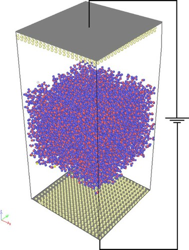
A final configuration of the equilibrated trajectory was placed at the centre of two face-centred-cubic (FCC) Pt electrodes, each consisting of three Pt layers. We considered Pt electrodes as it is the most studied metal at water interfaces, where Pt is studied using both computationally (classical and first-principles Born–Oppenheimer molecular dynamics (BOMD) simulations) and experimentally [29–33]. Pt metal is an ideal electrode to our current work as it is considered as an inert metal toward oxidation [34] and does not need to account for the bond breaking and formation of water during the classical simulations [35]. Moreover, the nature of the electrode does not affect our finding as there is no direct contact between water and the electrode. A direct contact of the electrode with the water results in the water dissociation at the voltage of 1.23 V in theory (0.11 V nm⁻¹) but 1.8 V (0.16 V nm⁻¹) is needed in practice to overcome the activation barrier of the reaction [36,37].

All the metal layers have a lattice constant of 3.92 Å and are spatially frozen during the simulations. A snapshot of the simulation geometry is shown in Figure 1. Periodic boundary conditions were applied along the x–y plane and the direction normal was defined along the z-direction, perpendicular to the Pt (111) surfaces. Unlike the original CPM, which used 2d-periodic Ewald sums [38,39], 3d-periodic Ewald sums with shape corrections were used to improve the calculation speed [40], with a volume factor set to 3. The correction term to the usual 3d-periodic energy expression is given by $\frac{2\pi }{V}{\left(\sum _i{q}_i{z}_i\right)}^2$.

Figure 1. Representation of the simulation system of the constant potential method MD simulations; Left and right-side electrodes are negative and positive electrodes respectively. Colour scheme: Red-O, white-H, green-Pt.

The simulation cell dimensions were 55.5, 55.5, and 129 Å in x-, y-, and z-direction, respectively. Pt electrodes were placed 30 Å above the water surface and thus were located at −58 and 58 Å in the z-axis. The distance of 30 Å from the surface was chosen to be larger than a certain jump-in distance of ∼20 Å to prevent water molecules from jumping to the electrode [26].

Na⁺ and Cl⁻ ions were placed on the top (surface directed towards positive electrode) and bottom (surface directed towards positive electrode) layers of the water. Lorentz–Berthelot mixing rules, σ_ij = (σ_i + σ_j)/2, ε_ij = (ε_iε_j)^1/2 were applied to calculate cross interatomic LJ interactions. In this work, the minimum and maximum applied potentials corresponded to the minimum and maximum electric fields of 0 V nm⁻¹ and 1.2 V nm⁻¹ respectively. It should be noted here that these values represent the external electric field applied by the electrodes. The total electric field depicted later in this work is the sum of the external field and the field induced in the water slap. For each case, the system is equilibrated for 2.5 ns, and properties were computed every 1000 ps for the analysis.

3. Results and discussions

The equilibrated final configurations obtained with a potential difference of 0 V nm^−1–1.2 V nm⁻¹ from CPM simulations are shown in Figure 2(a–f). These configurations delineate the instantaneous charges formed on saltwater and Pt (111) surface which were maintained at a constant potential difference. The quantity of the in-situ charge on both the electrodes was induced by the Coulombic interactions between the Pt atoms and prompt configuration of the charges in the total system. All the atoms are colour-coded with blue and red colours represent the negative and positive charges in Figure 2(a–f), respectively. To get a clear visual insight of the charge density on the electrode atoms at the relatively lower and higher voltages, the charges range of [–0.001e, 0.001e] is calculated for 0 V nm⁻¹–0.5 V nm⁻¹ (see Figure 2(a–c)) and [–0.003e, 0.003e].

Figure 2. (a–f) are snapshots of CPM simulations at (0 V nm⁻¹, 0.1 V nm⁻¹, 0.5 V nm⁻¹, 0.75 V nm⁻¹, 1.0 V nm⁻¹ 1.2 V nm⁻¹) respectively, temperature 298 K. Colour scheme on all atoms represents the instantaneous charge on the atoms: blue-negative charge and red-positive charge. (a–c) snapshots are shown within the charge range of [−0.001e to 0.001e] and (d–f) snapshots are within the charge range of [−0.003e to 0.003e] for the sake of clarity. Three-layered atoms at both ends correspond to Pt and middle atoms correspond to water and NaCl.

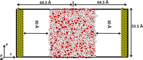
Figure 3. Electric potential profiles for the application of 0 V nm⁻¹, 0.1 V nm⁻¹, 0.5 V nm⁻¹, 0.75 V nm⁻¹, 1.0 V nm⁻¹, and 1.2 V nm⁻¹ potential differences on the Pt electrodes. The dotted straight lines parallel to y-axis represent the limits of the water slab.

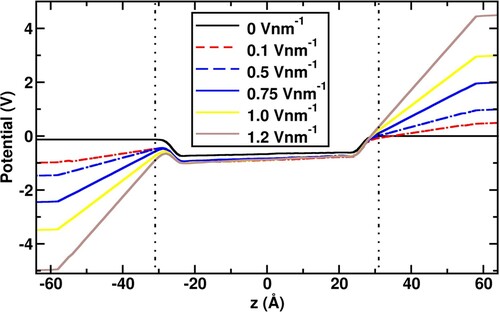
Figure 4. (a) 1D electric field profiles along the z-direction generated by the application of 0 V nm⁻¹ and 1.2 V nm⁻¹ electric potential difference on the saltwater system; (b) Electric field generated at the anode’s interface (top panel) and cathode’s interface (bottom panel) as functions of external applied fields.

Figure 5. (a) Trajectory of the maximum value of z-coordinate of surface water molecules that aligned towards both the electrodes at the extremum applied electric potentials differences of 0 and 1.2 V nm⁻¹. The top and bottom panels represent the z-length values at the upper and bottom interfaces.; (b) Time-averaged z-coordinate of the surface molecules as a function of the external electric field. The top and bottom panels correspond to the z-length values at the anode and cathode interfaces, respectively.

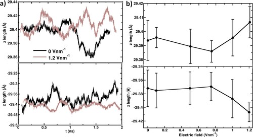
Figure 6. Comparison of surface tension calculated using the CPM method and the direct approach (constant electric field). Standard deviations (error bars) are obtained from the block average of five blocks of each consisting of 0.5 ns trajectory data.

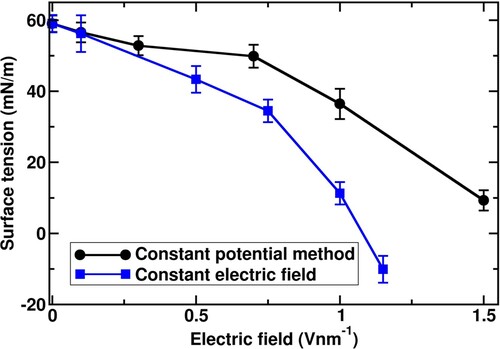
Figure 7. Pressure tensor along x-, y-, and z-direction on the interface model obtained from (a) constant potential method and (b) constant electric field MD simulations.

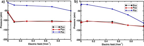
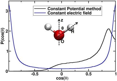
Figure 8. Probability distribution of angles between z-axis and $\overrightarrow{OH}$ vector (see inset) obtained H₂O in CPM and CFM simulations at 1.2 V nm⁻¹. Inset: Illustration of the angle between the reference axis (z-axis) and $\overrightarrow{OH}$ vector.

As shown in Figure 2, the magnitude of the charge on the Pt electrode increases with the applied constant potential. To check the behaviour of the constant potential implementation in our MD simulations while modelling the near electrode saltwater surface system, 1-dimensional electrostatic potential profiles were calculated using the following equation. (4) $\psi (z)=-{\int }_0^z\text{d}{z}^{\mathrm{\prime }}{\int }_0^{z^{\mathrm{\prime }}}\frac{\rho (z^{\mathrm{\prime }\mathrm{\prime }})}{{\epsilon }_0}\text{d}{z}_{}^{\mathrm{\prime }\mathrm{\prime }}$(4) where ε₀ is the vacuum permittivity and ρ is the charge distribution along the z-axis.

All the calculated electric potential profiles are shown in Figure 3 depicting the gap between the electrodes. The linear change of the electric potential in the bulk of the water slab is consistent with the 1-dimensional solution of the Laplace equation, confirming that the CPM captures the continuum limit correctly. The small non-zero slopes of the potential in the bulk slab region of the z-axis [–2.2, 2.2 nm] are due to the high permittivity of water. The potential changes non-linearly at the interface due to surface polarisation.

To calculate the electric field generated by applying constant potential, the derivative of the electrostatic potential with respect to the z-direction length using the following equation. (5) $E=\frac{\mathrm{\partial }\psi }{\mathrm{\partial }z}$(5)

The calculated electric fields by the application of 0 V nm⁻¹ and 1.2 V nm⁻¹ on the saltwater system are shown in Figure 4(a). The electric field obtains its maximum value on a single monolayer at the interface of the saltwater system. The peak electric field generated at the interface upon the application from 0 to 1.2 V nm⁻¹ is shown in Figure 4(b). The top panel in Figure 4(b) represents the upper interface facing the anode, while the lower panel represents the lower interface facing the cathode. As the external potential is increased, the maximum electric field at the anode’s interface increases while at the cathode’s interface decreases. This can be explained by the variation in the charge density on the monolayer at the interface region. With increasing the external potential applied to the electrodes, charge density represented by Na⁺ ions accumulates at the interface facing the cathode, causing a weaker field at the interface facing the cathode. Cl⁻ ions on the other hand do not follow the same behaviour. According to Smith et al., Cl⁻ ions possess a more favourable solvation free energy than Na⁺ ions in the liquid water phase at 298 K [41] which was proved theoretically and experimentally. Therefore, the Cl⁻ ions spend most of the trajectory time in the bulk, making the anode’s interface act as if it is pure water, where the interfacial electric field increases as the externally applied field are increased.

Further, to understand the changes in the structural characteristics of the interface with that of the bulk system, mass density profiles as a function of z-length were calculated at different constant potential MD simulations. The profiles are calculated by binning the simulation box along z-length and averaging the quantity of interest within each bin over the xyδz volume and bin size is of δz = 1.0 Å. The saltwater is situated in the region from −30 Å to 30 Å with a thickness of ∼60 Å and the electrode densities are identified at higher ends. The bulk density of the saltwater system at 0 V potential difference (T = 298 K) was calculated as 1.0 g cm⁻³, which agrees well with the reported literature values [42]. An insignificant decrease in the bulk density of 0.6%, was observed upon application of the external potential 0–1.2 V nm⁻¹. This observation also agrees well with reports by Nikzad et al. [43] and Yong et al., who reported the percentage difference in the density of water to be 0.5% for values similar to those investigated in this work [26]. Essentially, this indicates that the decrease in the bulk density is identical whether the CPM or the CFM is used.

The deformation of the water structure upon the application of external potential is examined by calculating the average z coordinate of the surface water molecules that direct towards both the electrodes as a function of time, which is shown in Figure 5(a,b). We used in-house codes that complement the established identification of truly interfacial molecules (ITIM) algorithm [44] for these analyses. It is evident that the fluctuations in the z values increase from 0 to 1.2 V nm⁻¹. This increase explains the reduction in the density of the water. Moreover, the enhanced fluctuations in the surface structure lead to disturbances in the cohesive forces between the water molecules at the surface, which affects surface tension. This phenomenon is quantitatively described in the following text.

The surface tension was computed for the saltwater (as described in Section 2) upon the application of CPM and CFM. The coefficients were calculated at different electric potentials to quantify the effect of the external electrostatic potential on the liquid–vapor interface. The pressure tensor was calculated by LAMMPS, which was then used to calculate the surface tension as shown in equation 6. (6) $\gamma =\frac{L_z}{2}\left\{P_{zz}-\frac{P_{xx}+P_{yy}}{2}\right\}$(6) where L_z is the length of the box, P_xx, P_yy, and P_zz are the three diagonal components of the pressure tensor along the x-, y-, and z-directions, respectively. The values obtained for the surface tension are shown in Figure 6.

In all cases, the surface tension decreases with increasing voltages over the investigated range of applied potentials. This is due to the disturbance to the cohesive interaction between water molecules at the interface as observed in the deformation of the water surface.

The CPM predictions of the surface tensions are in good qualitative agreement with the CFM where decreasing surface tension by increasing the electric fields from 0 to 1.2 V nm⁻¹. Our CFM results are in good agreement with those reported values by Nikzad et al. [43]. Quantitatively, however, there is a considerable difference observed in the variation between the CFM and CPM calculated surface tension values. The CPM MD simulations showed a weaker variation in the surface tension values compared to that of the reported values as shown in Figure 6.

In both CPM and CFM, the electric field is directed perpendicular to the saltwater slab surfaces which is along the z-axis direction. Hence, the difference between these two simulation methods stems from the induced pressure tensor along the z-axis, P_zz (see Equation (6)) as shown in Figure 7. The weaker decreasing trend in the P_zz values dominates the variation in the surface tensions as per Equation (6) with increasing the electric field.

The difference in the P_zz originates from the virial component of the pressure. In CFM simulations as the electric field is increased, the structure of the water slab is distorted and water molecules align in the direction of the electric field, as reported by Nikzad et al., which gradually converts to cylindrical shape by vanishing the interface along the z-direction. To understand the orientation of water molecules, the angle distribution function of water configurations obtained using both methods at 1.2 V nm⁻¹ was analyzed. The angle distribution between electric field applied axis, z-axis and $\overrightarrow{OH}$ vector of H₂O was calculated and is shown in Figure 8. In CPM simulations, water molecules display orientational freedom with a span of a range between 0˚ to 104˚ and a preferred angle of 30˚. However, in CFM simulations, all the water molecules orient parallel to the reference axis, z-axis, and show only angles of 0˚ or 180˚. It clearly explains that the water molecules orient along the applied field in CFM simulations at increased fields, in good agreement with the report of Nikzad et al. [43]. Whereas in CPM simulations, the preferred orientation of water molecules along with the applied voltage is not prominent. This is due to the shielding of the applied electric field by the water slab, an effect which is captured in the CPM method but not in the CFM method. Thus, the tensor component along the z-axis gradually decreases because of weakening the molecular structure by breaking the hydrogen bonds with the assistance of the higher fields.

3.1. Interfacial mobility calculations

The CPM MD simulations were carried out in an attempt to calculate the interfacial mobilities of Na⁺ and Cl⁻ ions. To do so the displacements of the ions in response to the applied potential difference were analyzed. The saltwater system was divided into three regions: (i) interface orients towards the anode where Na⁺ ions present at this interface in the starting configuration, (ii) interface directs towards the cathode where Cl⁻ ions present at this interface in the starting configuration, and (iii) bulk water region. The displacement of the individual six Na⁺ and Cl⁻ ions along the z-direction was calculated at 0 to 1.2 V nm⁻¹.

It was observed that both the ions tend to stay most of the simulation time in the bulk region, which can be explained as it is more energetically favourable for the ions to have a complete hydration shell, which cannot occur on the interface. In addition, the ions drift to the interfaces was observed to be independent of the applied electric potential. The absence of a clear trend in the displacement of ions was attributed to poor statistical sampling considering that the ions have a short residence time in the interface regions and that their number is small, which was to maintain the infinite dilution approximation. Therefore, for the CPM method to compute the interfacial mobilities much longer trajectories are required in comparison to typical trajectories required for the computation of other physical properties.

CFM simulations provided clear trend in the displacement of ions due to the better statistical sampling as the ions-solvent interaction is continuous over the entire simulation time. Nevertheless, the mobilities computed using this approach represent the bulk mobilities, which were reported in many previous works. To capture interfacial mobilities, the simulation should simultaneously take into account the variation of the electric local electric field and the broken hydration shell at the interface, which is not possible using the standard application of CFM method.

4 Conclusions

In this work, the Constant Potential Method (CPM) was implemented to study two physical properties of a slab of liquid water with a total of 12 ions of Na⁺ and Cl⁻, subject to an externally applied potential. These were the surface tension and the interfacial mobilities of Na⁺ and Cl⁻. The surface tension was compared to that computed using the more conventional constant field method, where a constant Coulombic force is applied to all charges in the system under investigation.

It was reported that the surface tensions followed a similar trend in both methods used, showing a decrease in its value as the external potential was increased. However, the CPM method showed a weaker variation by a factor of 36% in comparison to that of the CFM. This was attributed to the weaker decline in the normal pressure that was applied on the saltwater slab with increasing external field causing the less cohesive force disturbance between surface water molecules.

Despite the possibility of computing the interfacial mobility of the ions in the water, it was shown to not be doable on trajectories of few nanoseconds. This is due to the ions spending most of the trajectory time in the bulk region of the slab where it is more energetically favourable, as they are surrounded by a hydration shell.

Disclosure statement

No potential conflict of interest was reported by the author(s).

Additional information

Funding

The authors acknowledge the support of the Engineering and Physical Sciences Research Council [project EP/T000104/1].

References

- P. Teng, D. Tian, H. Fu and S. Wang, Mater. Chem. Front. 4, 140–154 (2020). doi:https://doi.org/10.1039/C9QM00458K.
- M. Tokman, J.H. Lee, Z.A. Levine, M.-C. Ho, M.E. Colvin, P.T. Vernier and J.M. Sanchez-Ruiz, PLoS One. 8, e61111 (2013). doi:https://doi.org/10.1371/journal.pone.0061111.
- B.-B. Wang, X.-D. Wang, Y.-Y. Duan and M. Chen, Int. J. Heat. Mass. Transf. 73, 533–541 (2014). doi:https://doi.org/10.1016/j.ijheatmasstransfer.2014.02.034.
- A. Campione, L. Gurreri, M. Ciofalo, G. Micale, A. Tamburini and A. Cipollina, Desalination. 434, 121–160 (2018). doi:https://doi.org/10.1016/j.desal.2017.12.044.
- L. Giuliani, L. De Angelis, G. Diaz Bukvic, M. Zanini, F. Minotti, M.I. Errea and D. Grondona, J. Appl. Phys. 127, 223303 (2020). doi:https://doi.org/10.1063/5.0005197.
- I.M. Svishchev and P.G. Kusalik, J. Am. Chem. Soc. 118, 649–654 (1996). doi:https://doi.org/10.1021/ja951624l.
- E.C. Neyts and P. Brault, Plasma. Process. Polym. 14, 1600145 (2017). doi:https://doi.org/10.1002/ppap.201600145.
- M. Kiselev and K. Heinzinger, J. Chem. Phys. 105, 650–657 (1996). doi:https://doi.org/10.1063/1.471921.
- W. Sun, Z. Chen and S. Huang, J. Shanghai Univ. (English Ed.). 10, 268–273 (2006). doi:https://doi.org/10.1007/s11741-006-0127-1.
- N.K. Karna, A. Rojano Crisson, E. Wagemann, J.H. Walther and H.A. Zambrano, Phys. Chem. Chem. Phys. 20, 18262–18270 (2018). doi:https://doi.org/10.1039/C8CP03186J.
- A. Lohrasebi and S. Rikhtehgaran, Nano Res. 11, 2229–2236 (2018). doi:https://doi.org/10.1007/s12274-017-1842-6.
- S. Murad, J. Chem. Phys. 134, 114504 (2011). doi:https://doi.org/10.1063/1.3565478.
- Y. Tsori and L. Leibler, Proc. Natl. Acad. Sci. 104, 7348–7350 (2007). doi:https://doi.org/10.1073/pnas.0607746104.
- J. Peng, D. Cao, Z. He, J. Guo, P. Hapala, R. Ma, B. Cheng, J. Chen, W.J. Xie, X.-Z. Li, P. Jelínek, L.-M. Xu, Y.Q. Gao, E.-G. Wang and Y. Jiang, Nature. 557, 701–705 (2018). doi:https://doi.org/10.1038/s41586-018-0122-2.
- S.H. Lee and J.C. Rasaiah, J. Phys. Chem. 100, 1420–1425 (1996). doi:https://doi.org/10.1021/jp953050c.
- S.K. Reed, O.J. Lanning and P.A. Madden, J. Chem. Phys. 126, 84704 (2007). doi:https://doi.org/10.1063/1.2464084.
- Z. Wang, Y. Yang, D.L. Olmsted, M. Asta and B.B. Laird, J. Chem. Phys. 141, 184102 (2014). doi:https://doi.org/10.1063/1.4899176.
- Z. Wang, D.L. Olmsted, M. Asta and B.B. Laird, J. Phys. Condens. Matter. 28, 464006 (2016). doi:https://doi.org/10.1088/0953-8984/28/46/464006.
- J. Vatamanu, D. Bedrov and O. Borodin, Mol. Simul. 43, 838–849 (2017). doi:https://doi.org/10.1080/08927022.2017.1279287.
- K.A. Dwelle and A.P. Willard, J. Phys. Chem. C. 123, 24095–24103 (2019). doi:https://doi.org/10.1021/acs.jpcc.9b06635.
- H.J.C. Berendsen, J.R. Grigera and T.P. Straatsma, J. Phys. Chem. 91, 6269–6271 (1987). doi:https://doi.org/10.1021/j100308a038.
- J. Zielkiewicz, J. Chem. Phys. 123, 104501 (2005). doi:https://doi.org/10.1063/1.2018637.
- J.R. Errington and A.Z. Panagiotopoulos, J. Phys. Chem. B. 102, 7470–7475 (1998). doi:https://doi.org/10.1021/jp982068v.
- Y.D. Fomin, V.N. Ryzhov, E.N. Tsiok and V.V. Brazhkin, Sci. Rep. 5, 14234 (2015). doi:https://doi.org/10.1038/srep14234.
- I.S. Joung and T.E. Cheatham, J. Phys. Chem. B. 112, 9020–9041 (2008). doi:https://doi.org/10.1021/jp8001614.
- P. Yang, Z. Wang, Z. Liang, H. Liang and Y. Yang, Chinese J. Chem. 37, 1251–1258 (2019). doi:https://doi.org/10.1002/cjoc.201900270.
- S. Plimpton, J. Comput. Phys. 117, 1–19 (1995). doi:https://doi.org/10.1006/jcph.1995.1039.
- T.R. Gingrich and M. Wilson, Chem. Phys. Lett. 500, 178–183 (2010). doi:https://doi.org/10.1016/j.cplett.2010.10.010.
- T. Ikeshoji, M. Otani, I. Hamada, O. Sugino, Y. Morikawa, Y. Okamoto, Y. Qian and I. Yagi, AIP. Adv. 2, 32182 (2012). doi:https://doi.org/10.1063/1.4756035.
- X. Xia and M.L. Berkowitz, Phys. Rev. Lett. 74, 3193–3196 (1995). doi:https://doi.org/10.1103/PhysRevLett.74.3193.
- K. Heinzinger, Pure Appl. Chem. 63, 1733–1742 (1991). doi:https://doi.org/10.1351/pac199163121733.
- H. Ogasawara, B. Brena, D. Nordlund, M. Nyberg, A. Pelmenschikov, L.G.M. Pettersson and A. Nilsson, Phys. Rev. Lett. 89, 276102 (2002). doi:https://doi.org/10.1103/PhysRevLett.89.276102.
- B. Shi, M.V. Agnihotri, S.-H. Chen, R. Black and S.J. Singer, J. Chem. Phys. 144, 164702 (2016). doi:https://doi.org/10.1063/1.4945760.
- R. Chen, C. Yang, W. Cai, H.-Y. Wang, J. Miao, L. Zhang, S. Chen and B. Liu, ACS Energy Lett. 2, 1070–1075 (2017). doi:https://doi.org/10.1021/acsenergylett.7b00219.
- A.P. Willard, D.T. Limmer, P.A. Madden and D. Chandler, J. Chem. Phys. 138, 184702 (2013). doi:https://doi.org/10.1063/1.4803503.
- X. Li, J. Yu, J. Jia, A. Wang, L. Zhao, T. Xiong, H. Liu and W. Zhou, Nano Energy. 62, 127–135 (2019). doi:https://doi.org/10.1016/j.nanoen.2019.05.013.
- L. Wang, Y. Lu, N. Han, C. Dong, C. Lin, S. Lu, Y. Min and K. Zhang, Small. 17, 2100400 (2021). doi:https://doi.org/10.1002/smll.202100400.
- M. Kawata, M. Mikami and U. Nagashima, J. Chem. Phys. 115, 4457–4462 (2001). doi:https://doi.org/10.1063/1.1395564.
- S.W. De Leeuw and J.W. Perram, Mol. Phys. 37, 1313–1322 (1979). doi:https://doi.org/10.1080/00268977900100951.
- I.-C. Yeh and M.L. Berkowitz, J. Chem. Phys. 111, 3155–3162 (1999). doi:https://doi.org/10.1063/1.479595.
- E.J. Smith, T. Bryk and A.D.J. Haymet, J. Chem. Phys. 123, 34706 (2005). doi:https://doi.org/10.1063/1.1953578.
- J. Alejandre, D.J. Tildesley and G.A. Chapela, J. Chem. Phys. 102, 4574–4583 (1995). doi:https://doi.org/10.1063/1.469505.
- M. Nikzad, A.R. Azimian, M. Rezaei and S. Nikzad, J. Chem. Phys. 147, 204701 (2017). doi:https://doi.org/10.1063/1.4985875.
- L.B. Pártay, G. Hantal, P. Jedlovszky, Á. Vincze and G. Horvai, J. Comput. Chem. 29, 945–956 (2008). doi:https://doi.org/10.1002/jcc.20852.