Spin–orbit coupling matrix elements from the explicitly connected expressions of the response functions within the coupled-cluster theory

Abstract

In this work, we present a coupled cluster-based approach to the computation of the spin–orbit coupling matrix elements. The working expressions are derived from the quadratic response function with the coupled-cluster parametrisation, using the auxiliary excitation operator S. Systematic approximations are proposed with the CCSD and CC3 levels of theory. The new method is tested by computing lifetimes of several electronic states of Ca, Sr and Ba atoms, with Gaussian and Slater basis sets. The results are compared with available theoretical and experimental data.

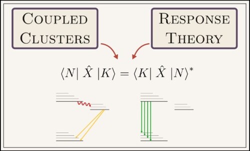
GRAPHICAL ABSTRACT

Keywords:

• Coupled clusters
• spin–orbit interaction
• transition moments
• transition probability
• lifetimes

1. Introduction

The spin–orbit (SO) interaction is a relativistic effect that plays a crucial role in the description of the electronic structure of heavy atoms. It causes the fine structure splitting and mixing of states with different multiplicities. In heavy atoms, the energy separation of the multiplet states due to the SO interaction becomes comparable to the energy separation between different electronic states. The second effect on the electronic structure is the mixing of states with different multiplicities causing radiative (phosphorescence) and nonradiative (intersystem crossing) decays. Contributions of spin–forbidden transitions are crucial for the computation of lifetimes of electronic states [1].

In this work, we focus on the spin–orbit coupling operators introduced in the framework of effective core potentials (SO ECP). This approximation was first proposed by Pitzer [2] and Schwartz [3], and is used in this work in the Pitzer and Winter formulation [4]. The effective Hamiltonian is given by (1) $H_{\mathrm{S}\mathrm{O}}=\sum _{l=1}^{l_{\mathrm{m}\mathrm{a}\mathrm{x}}}{\xi }_l\left(r\right)P_l\overrightarrow{l}\cdot \overrightarrow{s}{P}_l,$(1) where ${\xi }_l\left(r\right)$ is a radial potential and $P_l=\sum _{m_l}|l,m_l〉〈l,m_l|$ is the projection operator onto spherical harmonics with angular momentum l placed at a given pseudopotential centre.

In high-resolution spectroscopy, interpretation of the experimental spectra requires a theory that effectively includes both the relativistic effects and the electron correlation at a high level. In this work, we propose computing the SO coupling matrix elements within the coupled cluster (CC) approach to the response theory. There exist two approaches to the coupled cluster response theory. The first one, introduced in 1977 by Monkhorst [5,6] and extended by Bartlett et al. [7–10], is based on differentiation of the CC energy expression. Later, Koch et al. [11–14] derived the time-averaged quasi-energy Lagrangian technique. Within this approach, the expressions for the linear, quadratic, and cubic response functions [14], transition moments [15], spin–orbit coupling matrix elements [16,17], and many other properties [18], at the CC2 [19,20], CCSD [12], and CC3 levels [21,22] of theory were proposed. We will refer to this method as time-dependent CC theory (TD-CC).

In this work, we use the alternative approach in which one computes molecular properties directly from the average value of an operator X, using the auxiliary excitation operator S. Parenthetically, we note that this method, referred to as XCC, should not be confused with the approach of Bartlett and Noga [23] of the same name. The operator S was introduced in the context of CC theory in the works of Arponen et al. [24–26]. The authors defined the operator S through a set of nonlinear equations with no systematic scheme of approximations. In 1993, Jeziorski and Moszynski [27] proposed a different expression for the operator S that satisfies a set of linear equations and can be systematically approximated. Starting from the formula for the average value of X expressed through a finite series of commutators, the XCC method was extended to the computation of various electronic properties: electrostatic [28] and exchange [29] contributions to the interaction energies of closed-shell systems, the polarisation propagator [30], first-order molecular properties [31], static and dynamic dipole polarisabilities [32], and transition moments between excited states [33,34]. There is also a series of publications by Korona et al. on the computation of symmetry-adapted perturbation theory (SAPT) contributions [35–38]. An extensive review of the XCC methodology was recently published [39].

The XCC approach is straightforward in the sense that one makes use of the fundamental expression for the expectation value of an operator known from quantum mechanics. However, as the exact electronic wave function is approximated by the CC Ansatz, one encounters the problem of an infinite series expansion originating from the presence of the operator $T^{†}$. The introduction of the auxiliary operator S allows to overcome the problem. One proceeds in a similar manner for higher-order properties. As a result, all XCC properties are Hermitian irrespectively of the truncation scheme adopted for the cluster operator T. The only possible source of Hermiticity violation is the truncation of the auxiliary operator S. In other words, one can approach the Hermitian result in a controlled way by including higher-order corrections to S, even if the operator T itself is not exact. To the best of our knowledge, this is not the case in the TD-CC method, where any truncation of the cluster operator T automatically leads to the violation of the Hermiticity. We stress that preservation of the Hermitian nature of the theory is especially important in the calculation of the transition moments, where its violation can lead to an unphysical result, e.g. negative values of a transition strength [34]. Besides this favourable property of the XCC theory, there are also some computational advantages in comparison with the widely used TD-CC method. In fact, in the XCC theory, there is no need to solve separate equations for the so-called Λ amplitudes and the auxiliary operator S is calculated in a one-step procedure using a rapidly converging commutator expansion in combined powers of T and $T^{†}$. This makes the proposed approach less computationally demanding than TD-CC. Finally, it is worth pointing out that calculation of spin–orbit coupling matrix elements using CC models with explicit inclusion of triple excitations has not been reported thus far in the literature.

2. XCC theory

In CC theory [40–43], the ground state wave function ${\mathrm{\Psi }}_0$ is represented by the exponential ansatz ${\mathrm{\Psi }}_0=e^T\mathrm{\Phi }$, where Φ is the Slater determinant and the cluster operator T is a sum of n-tuple excitation operators (2) $T=\sum _{n=1}^N{T}_n,$(2) where N is the number of electrons. Each of the cluster operators $T_n$ is represented by (3) $T_n=\frac{1}{n!}\sum _{{\mu }_n}^N{t}_{{\mu }_n}{\mu }_n,$(3) and ${\mu }_n$ stands for the product of the n singlet excitation operators $E_{ai}$ [44]. The indices $a,b,c\dots$, $i,j,k\dots$ and $p,q,r\dots$ denote the virtual, occupied, and general orbitals, respectively.

In the XCC method molecular properties are computed with the use of the auxiliary excitation operator $S=S_1+S_2+S_3+\cdots$ defined as (4) $e^S\mathrm{\Phi }=\frac{e^{T^{†}}{e}^T\mathrm{\Phi }}{〈e^{T^{†}}{e}^T〉}.$(4) The S operator satisfies a set of linear equations expressed through a finite series of commutators [27] (5) $\begin{array}{rl}{S}_n& =T_n-\frac{1}{n}{\hat{\mathcal{P}}}_n\left(\sum _{k=1}\frac{1}{k!}\right[\tilde{T}{}^{†},T{]}_k)\\ & -\frac{1}{n}{\hat{\mathcal{P}}}_n\left(\sum _{k=1}\sum _{m=0}\frac{1}{k!}\frac{1}{m!}\right[[\tilde{S},T^{†}{]}_k,T{]}_m),\end{array}$(5) where (6) $\tilde{T}=\sum _{n=1}^{N}n{T}_n,\tilde{S}=\sum _{n=1}^{N}n{S}_n,$(6) and $[A,B{]}_k$ denotes a k-tuply nested commutator. The superoperator ${\hat{\mathcal{P}}}_n\left(X\right)$ yields the excitation part of X (7) ${\hat{\mathcal{P}}}_n\left(X\right)=\frac{1}{n!}\sum _{{\mu }_n}〈{\mu }_n|X〉{\mu }_n$(7) and $〈{\mu }_n|$ and $|{\nu }_m〉$ constitute a biorthonormal basis $〈{\mu }_n|{\nu }_m〉={\delta }_{{\mu }_n{\nu }_m}$ . The expression for the transition moment is derived from the quadratic response function, ${〈〈X;Y,Z〉〉}_{{\omega }_Y,{\omega }_Z}$, which describes the response of an observable X to periodic perturbations Y and Z with frequencies ${\omega }_Y$ and ${\omega }_Z$, respectively. The explicit form of the response function written as a sum over states reads [14] (8) $\begin{array}{rl}& 〈〈X;Y,Z〉{〉}_{{\omega }_Y,{\omega }_Z}\\ & =P_{XYZ}(\sum _{\begin{array}{c}{K}^{\prime }=1\\ N^{\prime }=1\end{array}}\frac{〈{\mathrm{\Psi }}_0\left|Y\right|{\mathrm{\Psi }}_{K^{\prime }}〉[〈{\mathrm{\Psi }}_{K^{\prime }}\left|X\right|{\mathrm{\Psi }}_{N^{\prime }}〉}{({\omega }_{K^{\prime }}+{\omega }_Y)({\omega }_{N^{\prime }}-{\omega }_Z)}\\ & +\sum _{\begin{array}{c}{K}^{\prime }=1\\ N^{\prime }=1\end{array}}\frac{{\delta }_{K^{\prime }{N}^{\prime }}〈{\mathrm{\Psi }}_0\left|X\right|{\mathrm{\Psi }}_0〉]〈{\mathrm{\Psi }}_{N^{\prime }}\left|Z\right|{\mathrm{\Psi }}_0〉}{({\omega }_{K^{\prime }}+{\omega }_Y)({\omega }_{N^{\prime }}-{\omega }_Z)}),\end{array}$(8) where the operator $P_{XYZ}$ symmetrises the expression with respect to exchange of the indices X, Y, and Z. The indices $K^{\prime }$ and $N^{\prime }$ run over all possible excited states with excitation energies ${\omega }_{K^{\prime }}$ and ${\omega }_{N^{\prime }}$. The transition moment ${\mathcal{T}}_{KN}^X$ between the excited states K and N, with $K\ne N$, is computed as a residue of the quadratic response function (9) $\begin{array}{rl}& \underset{{\omega }_Y\to -{\omega }_K}{lim}({\omega }_K+{\omega }_Y)\underset{{\omega }_Z\to {\omega }_N}{lim}({\omega }_N-{\omega }_Z){〈〈X;Y,Z〉〉}_{{\omega }_Y,{\omega }_Z}\\ & =〈{\mathrm{\Psi }}_0\left|Y\right|{\mathrm{\Psi }}_K〉〈{\mathrm{\Psi }}_K\left|X_0\right|{\mathrm{\Psi }}_N〉〈{\mathrm{\Psi }}_N\left|Z\right|{\mathrm{\Psi }}_0〉\\ & ={\mathcal{T}}_{0K}^Y{\mathcal{T}}_{KN}^X{\mathcal{T}}_{N0}^Z.\end{array}$(9) where $X_0=X-〈X〉$ and $〈X〉=〈{\mathrm{\Psi }}_0\left|X\right|{\mathrm{\Psi }}_0〉$.

In our previous work [34], we employed the XCC formalism to express the quadratic response function in terms of the T and S operators. By using the first-order perturbed wave function (10) ${\mathrm{\Psi }}^{\left(1\right)}\left({\omega }_Y\right)={\mathcal{R}}_{{\omega }_Y}Y|{\mathrm{\Psi }}_0〉$(10) expressed through the resolvent ${\mathcal{R}}_{{\omega }_Y}$ (11) ${\mathcal{R}}_{{\omega }_Y}=\sum _{N^{\prime }=1}\frac{|N^{\prime }〉〈N^{\prime }|}{{\omega }_N+{\omega }_Y}.$(11)

Equation (8(8) $\begin{array}{rl}& 〈〈X;Y,Z〉{〉}_{{\omega }_Y,{\omega }_Z}\\ & =P_{XYZ}(\sum _{\begin{array}{c}{K}^{\prime }=1\\ N^{\prime }=1\end{array}}\frac{〈{\mathrm{\Psi }}_0\left|Y\right|{\mathrm{\Psi }}_{K^{\prime }}〉[〈{\mathrm{\Psi }}_{K^{\prime }}\left|X\right|{\mathrm{\Psi }}_{N^{\prime }}〉}{({\omega }_{K^{\prime }}+{\omega }_Y)({\omega }_{N^{\prime }}-{\omega }_Z)}\\ & +\sum _{\begin{array}{c}{K}^{\prime }=1\\ N^{\prime }=1\end{array}}\frac{{\delta }_{K^{\prime }{N}^{\prime }}〈{\mathrm{\Psi }}_0\left|X\right|{\mathrm{\Psi }}_0〉]〈{\mathrm{\Psi }}_{N^{\prime }}\left|Z\right|{\mathrm{\Psi }}_0〉}{({\omega }_{K^{\prime }}+{\omega }_Y)({\omega }_{N^{\prime }}-{\omega }_Z)}),\end{array}$(8) ) is rewritten in the following form: (12) ${〈〈X;Y,Z〉〉}_{{\omega }_Y,{\omega }_Z}=P_{XYZ}〈{\mathrm{\Psi }}^{\left(1\right)}\left({\omega }_Y\right)\left|X_0\right|{\mathrm{\Psi }}^{\left(1\right)}(-{\omega }_Z)〉.$(12) At this point, we introduce the coupled cluster parametrisation. The normalised ground-state wave function in this parametrisation is given by (13) $|{\mathrm{\Psi }}_0〉=\frac{|e^T\mathrm{\Phi }〉}{〈e^T\mathrm{\Phi }|e^T\mathrm{\Phi }{〉}^{\frac{1}{2}}},$(13) and the first-order wave function ${\mathrm{\Psi }}^{\left(1\right)}\left({\omega }_Y\right)$ is defined as (14) $\left|{\mathrm{\Psi }}^{\left(1\right)}\right({\omega }_Y)〉=({\mathrm{\Omega }}_0^Y+{\mathrm{\Omega }}^Y\left({\omega }_Y\right)\left)\right|{\mathrm{\Psi }}_0〉,$(14) through the excitation operator (15) ${\mathrm{\Omega }}^Y\left({\omega }_Y\right)={\mathrm{\Omega }}_1^Y\left({\omega }_Y\right)+{\mathrm{\Omega }}_2^Y\left({\omega }_Y\right)+\cdots$(15) where the nth excitation operator ${\mathrm{\Omega }}_n^Y\left({\omega }_Y\right)$ is (16) ${\mathrm{\Omega }}_n^Y\left({\omega }_Y\right)=\sum _{{\mu }_n}\frac{1}{n!}{O}_{{\mu }_n}^Y\left({\omega }_Y\right){\mu }_n.$(16) The operator ${\mathrm{\Omega }}^Y\left({\omega }_Y\right)$ is found from the linear response equation [30,32] (17) $〈{\mu }_n\left|\right[e^{-T}H{e}^T,{\mathrm{\Omega }}^Y\left({\omega }_Y\right)]+{\omega }_Y{\mathrm{\Omega }}^Y({\omega }_Y)+e^{-T}Y{e}^T〉=0.$(17) By transforming the ${\mu }_n$ index to the basis of the right, $r_N$, and left, $l_N$, eigenvectors of the CC Jacobian matrix [7,11,45] $A_{{\mu }_n{\nu }_m}=〈{\mu }_n|[e^{-T}H{e}^T,{\nu }_m]〉$ we arrive at (18) ${\omega }_N{O}_N^Y\left(\omega \right)+{\omega }_Y{O}_N^Y\left(\omega \right)+{\xi }_N^Y=0,$(18) where (19) ${\xi }_N^Y=〈l_N|e^{-T}Y{e}^T〉.$(19) With the explicit expression for $\mathrm{\Omega }\left({\omega }_V\right)$ given above, Equation (12(12) ${〈〈X;Y,Z〉〉}_{{\omega }_Y,{\omega }_Z}=P_{XYZ}〈{\mathrm{\Psi }}^{\left(1\right)}\left({\omega }_Y\right)\left|X_0\right|{\mathrm{\Psi }}^{\left(1\right)}(-{\omega }_Z)〉.$(12) ) is reformulated using the following identities: (20) $\begin{array}{rl}\mathrm{\Omega }\left({\omega }_Y\right)e^T& =e^T\mathrm{\Omega }\left({\omega }_Y\right),\\ e^{-S^{†}}\mathrm{\Phi }& =\mathrm{\Phi },\\ X\mathrm{\Phi }& =〈X〉\mathrm{\Phi }+\hat{\mathcal{P}}\left(X\right)\mathrm{\Phi },\\ \frac{〈e^T\left|X\right|e^T〉}{〈e^T|e^T〉}& =〈e^{S^{†}}{e}^{-T}X{e}^T{e}^{-S^{†}}〉.\end{array}$(20) The quadratic response function becomes (21) $\begin{array}{rl}& {〈〈X;Y,Z〉〉}_{{\omega }_Y,{\omega }_Z}\\ & =P_{XYZ}\sum _{\begin{array}{c}{K}^{\prime }=1\\ N^{\prime }=1\end{array}}\frac{〈e^{-T}Y{e}^T|l_{K^{\prime }}〉}{{\omega }_{K^{\prime }}+{\omega }_Y}\frac{〈l_{N^{\prime }}|e^{-T}Z{e}^T〉}{{\omega }_Z-{\omega }_{N^{\prime }}}\\ & \times 〈\kappa (r_{K^{\prime }},S,T)\left|e^{S^{†}}{e}^{-T}{X}_0{e}^T{e}^{-S^{†}}\right|\eta (r_{N^{\prime }},S)〉,\end{array}$(21) where we introduced a shorthand notation (22) $\begin{array}{rl}\kappa (r_{K^{\prime }},S,T)& =\hat{\mathcal{P}}\left(e^{-S}{e}^{T^{†}}{r}_{K^{\prime }}{e}^{-T^{†}}{e}^S\right),\\ \eta (r_{N^{\prime }},S)& =\hat{\mathcal{P}}\left(e^{S^{†}}{r}_{N^{\prime }}{e}^{-S^{†}}\right).\end{array}$(22) The transition moment between the excited states, ${\mathcal{T}}_{KN}^X$ is obtained from the residue of the quadratic response function [34] by dividing the RHS of Equation (9(9) $\begin{array}{rl}& \underset{{\omega }_Y\to -{\omega }_K}{lim}({\omega }_K+{\omega }_Y)\underset{{\omega }_Z\to {\omega }_N}{lim}({\omega }_N-{\omega }_Z){〈〈X;Y,Z〉〉}_{{\omega }_Y,{\omega }_Z}\\ & =〈{\mathrm{\Psi }}_0\left|Y\right|{\mathrm{\Psi }}_K〉〈{\mathrm{\Psi }}_K\left|X_0\right|{\mathrm{\Psi }}_N〉〈{\mathrm{\Psi }}_N\left|Z\right|{\mathrm{\Psi }}_0〉\\ & ={\mathcal{T}}_{0K}^Y{\mathcal{T}}_{KN}^X{\mathcal{T}}_{N0}^Z.\end{array}$(9) ) by $\left|{\mathcal{T}}_{0K}^Y{\mathcal{T}}_{N0}^Z\right|=\sqrt{\left|{\mathcal{T}}_{0K}^Y{|}^2\right|{\mathcal{T}}_{N0}^Z{|}^2}$. (23) ${\mathcal{T}}_{KN}^X=\frac{〈\kappa (r_K,S,T)\left|e^{S^{†}}{e}^{-T}{X}_0{e}^T{e}^{-S^{†}}\eta \right(r_N,S)〉}{\sqrt{〈\kappa (r_K,S,T)\left|\eta \right(r_K,S)〉〈\kappa (r_N,S,T)\left|\eta \right(r_N,S)〉}}.$(23) This expression was previously used to compute numerous dipole and quadrupole transitions between electronic states [34]. In this work, we employed ${\mathcal{T}}_{KN}^X$ to compute the spin–orbit transition moments.

3. Computational details

3.1. Spin-orbit coupling matrix elements in the spin-free formulation

The transition moments are usually represented in the literature via the line strength $\mathcal{S}$, which is defined as the square of the transition moment from the state $K\equiv 〈L^{\prime }{S}^{\prime }{J}^{\prime }|$ to the state $N\equiv |LSJ〉$ [46] (24) ${\mathcal{S}}_{KN}=|{\mathcal{T}}_{KN}^{\mathcal{T}{\mathcal{T}}^{\left(k\right)}}{|}^2=|〈L^{\prime }{S}^{\prime }{J}^{\prime }\left|\right|\mathcal{T}{\mathcal{T}}^{\left(k\right)}\left|\right|LSJ〉{|}^2.$(24) In the above notation, the transition moment $〈L^{\prime }{S}^{\prime }{J}^{\prime }\left|\right|\mathcal{T}{\mathcal{T}}^{\left(k\right)}\left|\right|LSJ〉$ is the reduced matrix element of the irreducible tensor operator $\mathcal{T}{\mathcal{T}}^{\left(k\right)}=({\mathcal{T}}_{-q}^{\left(k\right)},\dots ,{\mathcal{T}}_q^{\left(k\right)})$ of rank k with 2k + 1 components q, $q\in (-k,\dots ,k)$. L, S, and J are quantum numbers of the orbital, spin, and total angular momentum, respectively.

It is a common practice in ab initio calculations, including our XCC implementation, to compute the transition moments in the point group symmetry basis $|{}^{2S+1}{\mathrm{\Gamma }}^{m_S}〉$. In order to compare our results with the available experimental and theoretical results, we need to express the ${\mathcal{S}}_{KN}$ in the molecular point group symmetry basis. This is done by transforming the $|LSJ〉$ basis to the $|L{m}_{L}S{m}_S〉$ using angular momentum algebra. The correspondence between $|L{m}_{L}S{m}_S〉$ and $|{}^{2S+1}{\mathrm{\Gamma }}^{m_S}〉$ is straightforward.

The reduced matrix element of Equation (24(24) ${\mathcal{S}}_{KN}=|{\mathcal{T}}_{KN}^{\mathcal{T}{\mathcal{T}}^{\left(k\right)}}{|}^2=|〈L^{\prime }{S}^{\prime }{J}^{\prime }\left|\right|\mathcal{T}{\mathcal{T}}^{\left(k\right)}\left|\right|LSJ〉{|}^2.$(24) ) can be written explicitly by summing over all $m_J$ and $m_{J^{\prime }}$ in the $|LSJ{m}_J〉$ basis, (25) ${\mathcal{S}}_{KN}=\sum _{m_J,m_{J^{\prime }}}|〈L^{\prime }{S}^{\prime }{J}^{\prime }{m}_{J^{\prime }}|\mathcal{T}{\mathcal{T}}^{\left(k\right)}|LSJ{m}_J〉{|}^2.$(25) Instead of summing all these contributions, we exploit the Wigner–Eckart theorem and express ${\mathcal{S}}_{KN}$ through the 3−j coefficients as (26) $\begin{array}{rl}{\mathcal{S}}_{KN}& =|{\left(\right(-1{)}^{(J^{\prime }-m_{J^{\prime }})}\left(\begin{array}{ccc}{J}^{\prime }& k& J\\ -m_{J^{\prime }}& q& m_J\end{array}\right))}^{-1}\phantom{...}\\ & \times {\phantom{...}〈L^{\prime }{S}^{\prime }{J}^{\prime }{m}_{J^{\prime }}|{\mathcal{T}}_q^{\left(k\right)}|LSJ{m}_J〉\phantom{{\left(\begin{array}{ccc}{J}^{\prime }& k& J\\ -m_{J^{\prime }}& q& m_J\end{array}\right)}^{-1}}|}^2.\end{array}$(26) It is important to note that the line strength ${\mathcal{S}}_{KN}$ does not depend on the choice of $m_J$, so any non-trivial contribution to the reduced matrix element of Equation (26(26) $\begin{array}{rl}{\mathcal{S}}_{KN}& =|{\left(\right(-1{)}^{(J^{\prime }-m_{J^{\prime }})}\left(\begin{array}{ccc}{J}^{\prime }& k& J\\ -m_{J^{\prime }}& q& m_J\end{array}\right))}^{-1}\phantom{...}\\ & \times {\phantom{...}〈L^{\prime }{S}^{\prime }{J}^{\prime }{m}_{J^{\prime }}|{\mathcal{T}}_q^{\left(k\right)}|LSJ{m}_J〉\phantom{{\left(\begin{array}{ccc}{J}^{\prime }& k& J\\ -m_{J^{\prime }}& q& m_J\end{array}\right)}^{-1}}|}^2.\end{array}$(26) ) is sufficient to obtain the line strength. Next, we transform the $|LSJ{m}_J〉$basis to the $|L{m}_{L}S{m}_S〉$ basis, with the help of the Clebsch–Gordan coefficients (27) $|LSJ{m}_J〉=\sum _{m_L=-L}^L\sum _{m_S=-S}^S{C}_{L{m}_{L}S{m}_S}^{J{m}_J}|L{m}_{L}S{m}_S〉.$(27) Therefore, the expression for the line strength becomes (28) $\begin{array}{rl}{\mathcal{S}}_{KN}& =\left|\right(-1{)}^{(J^{\prime }-m_{J^{\prime }})}{\left(\begin{array}{ccc}{J}^{\prime }& k& J\\ -m_{J^{\prime }}& q& m_J\end{array}\right)}^{-1}\sum _{\begin{array}{c}{m}_L=-L\\ m_{L^{\prime }}=-L^{\prime }\end{array}}^{L,L^{\prime }}\sum _{\begin{array}{c}{m}_S=-S\\ m_{S^{\prime }}=-S^{\prime }\end{array}}^{S,S^{\prime }}\phantom{...}\\ & \times C_{L{m}_{L}S{m}_S}^{J{m}_J}{C}_{L^{\prime }{m}_{L^{\prime }}{S}^{\prime }{m}_{S^{\prime }}}^{J^{\prime }{m}_{J^{\prime }}}\\ & \times {\phantom{...}〈L^{\prime }{m}_{L^{\prime }}{S}^{\prime }{m}_{S^{\prime }}\left|{\mathcal{T}}_q^{\left(k\right)}\right|L{m}_{L}S{m}_S〉\phantom{{\left(\begin{array}{ccc}{J}^{\prime }& k& J\\ -m_{J^{\prime }}& q& m_J\end{array}\right)}^{-1}}\phantom{\sum _{\begin{array}{c}{m}_L=-L\\ m_{L^{\prime }}=-L^{\prime }\end{array}}^{L,L^{\prime }}}|}^2.\end{array}$(28)

The effective spin–orbit operator $H_{\mathrm{S}\mathrm{O}}$ from Equation (1(1) $H_{\mathrm{S}\mathrm{O}}=\sum _{l=1}^{l_{\mathrm{m}\mathrm{a}\mathrm{x}}}{\xi }_l\left(r\right)P_l\overrightarrow{l}\cdot \overrightarrow{s}{P}_l,$(1) ) is expressed through the triplet excitation operators (29) $\begin{array}{rl}{T}_{pq}^{11}& =-a_{p\alpha }^{†}{a}_{q\text{β}},\\ T_{pq}^{1-1}& =a_{p\text{β}}^{†}{a}_{q\alpha },\\ T_{pq}^{10}& =\frac{1}{\sqrt{2}}(a_{p\alpha }^{†}{a}_{q\alpha }-a_{p\text{β}}^{†}{a}_{q\text{β}}),\end{array}$(29) resulting in (30) $\begin{array}{rl}{H}_{\mathrm{S}\mathrm{O}}& =\sum _{pq}[(-\frac{i}{2}{V}_{pq}^x-\frac{1}{2}{V}_{pq}^y)T_{pq}^{11}\\ & +(\frac{i}{2}{V}_{pq}^x-\frac{1}{2}{V}_{pq}^y)T_{pq}^{1-1}+\frac{i}{2\sqrt{2}}{V}_{pq}^z{T}_{pq}^{10}],\end{array}$(30) where $V_{pq}^v$ (31) $V_{pq}^v=\frac{1}{i}\int {\varphi }_p^{\star }\left(\mathbf{\text{r}}\right)\xi \left(r\right)l_v{P}_l{\varphi }_q\left(\mathbf{\text{r}}\right)\mathrm{d}\mathbf{\text{r}}v\in (x,y,z).$(31) The transition moment ${\mathcal{T}}_{KN}^X$, where $X=H_{\mathrm{S}\mathrm{O}}$ , from state $K\equiv L^{\prime }{m}_{L^{\prime }}{S}^{\prime }{m}_{S^{\prime }}$ to $N\equiv L{m}_{L}S{m}_S$ becomes (32) $\begin{array}{rl}& 〈L^{\prime }{m}_{L^{\prime }}{S}^{\prime }{m}_{S^{\prime }}|H_{\mathrm{S}\mathrm{O}}|L{m}_{L}S{m}_S〉\\ & =\frac{1}{2}\sum _{pq}〈L^{\prime }{m}_{L^{\prime }}|(i{V}_{pq}^x+V_{pq}^y)|L{m}_L〉\\ & \times 〈S^{\prime }{m}_{S^{\prime }}|T_{pq}^{10}|S{m}_S〉\\ & +\frac{1}{2}\sum _{pq}〈L^{\prime }{m}_{L^{\prime }}|(-i{V}_{pq}^x+V_{pq}^y)|L{m}_L〉\\ & \times 〈S^{\prime }{m}_{S^{\prime }}|T_{pq}^{10}|S{m}_S〉\\ & +\frac{i}{2\sqrt{2}}\sum _{pq}〈L^{\prime }{m}_{L^{\prime }}|V_{pq}^z|L{m}_L〉〈S^{\prime }{m}_{S^{\prime }}|T_{pq}^{10}|S{m}_S〉.\end{array}$(32) To separate the spin and angular parts and use the spin-free formalism, we expressed the $m_S$-changing spin-tensor operators $T_{pq}^{11}$ and $T_{pq}^{1-1}$ in terms of $T_{pq}^{10}$ by the virtue of the Wigner–Eckart theorem.

3.2. Approximations

To compute the XCC properties, one needs to follow four independent steps: obtain the amplitudes T and S, compute the excitation amplitudes $r_N$, and finally use Equation (23(23) ${\mathcal{T}}_{KN}^X=\frac{〈\kappa (r_K,S,T)\left|e^{S^{†}}{e}^{-T}{X}_0{e}^T{e}^{-S^{†}}\eta \right(r_N,S)〉}{\sqrt{〈\kappa (r_K,S,T)\left|\eta \right(r_K,S)〉〈\kappa (r_N,S,T)\left|\eta \right(r_N,S)〉}}.$(23) ) to compute ${\mathcal{T}}_{KN}^X$. The calculation of the amplitudes T is done by any standard CC method. In this work, we use the coupled-cluster method limited to single and double excitations (CCSD) and the coupled-cluster method limited to single, double, and approximate triple excitations (CC3).

The expression for the auxiliary amplitudes S, Equation (5(5) $\begin{array}{rl}{S}_n& =T_n-\frac{1}{n}{\hat{\mathcal{P}}}_n\left(\sum _{k=1}\frac{1}{k!}\right[\tilde{T}{}^{†},T{]}_k)\\ & -\frac{1}{n}{\hat{\mathcal{P}}}_n\left(\sum _{k=1}\sum _{m=0}\frac{1}{k!}\frac{1}{m!}\right[[\tilde{S},T^{†}{]}_k,T{]}_m),\end{array}$(5) ), is a finite expansion, though it contains terms of high order in the fluctuation potential [27], i.e. in the sense of many-body perturbation theory (MBPT). To reduce the computational cost S can be systematically approximated while retaining the size-consistency [33]. Let $S_n\left(m\right)$ denote the n-electron part of S, where all contributions up to and including the order m of MBPT are accounted for. In the computations based on the CC3 model, we employ (33) $\begin{array}{rl}{S}_1\left(2\right)& =T_1,\\ S_1\left(3\right)& =S_1\left(2\right)+{\hat{\mathcal{P}}}_1\left(\right[T_1^{†},T_2\left]\right)+{\hat{\mathcal{P}}}_1\left(\right[T_2^{†},T_3\left]\right),\\ S_2\left(2\right)& =T_2,\\ S_2\left(3\right)& =S_2\left(2\right)+\frac{1}{2}{\hat{\mathcal{P}}}_2\left(\right[[T_2^{†},T_2],T_2\left]\right),\\ S_3\left(2\right)& =T_3,\end{array}$(33) where the CC3 equations for $T_1$, $T_2$ and $T_3$ are given by Koch et al. [21]. In the instances where the underlying model of the wave function is CCSD, we employ $S=S_1\left(3\right)+S_2\left(3\right)$ neglecting the terms containing $T_3$. The amplitudes $r_N$ are obtained from the EOM-CC3 or EOM-CCSD model depending on which approximation is used for the ground state, with the cost scaling as $N^7$ and $N^6$, respectively.

The most challenging problem is to systematically approximate the transition moment formula. In order to do so, we performed a commutator expansion of the numerator of Equation (23(23) ${\mathcal{T}}_{KN}^X=\frac{〈\kappa (r_K,S,T)\left|e^{S^{†}}{e}^{-T}{X}_0{e}^T{e}^{-S^{†}}\eta \right(r_N,S)〉}{\sqrt{〈\kappa (r_K,S,T)\left|\eta \right(r_K,S)〉〈\kappa (r_N,S,T)\left|\eta \right(r_N,S)〉}}.$(23) ) and assessed the importance of each term individually by order of its leading MBPT contribution. The formulas were derived automatically by the program paldus developed by one of us (AMT). Due to the computational and memory restrictions some additional approximations were used, as described below.

All terms resulting from commutator expansion of Equation (23(23) ${\mathcal{T}}_{KN}^X=\frac{〈\kappa (r_K,S,T)\left|e^{S^{†}}{e}^{-T}{X}_0{e}^T{e}^{-S^{†}}\eta \right(r_N,S)〉}{\sqrt{〈\kappa (r_K,S,T)\left|\eta \right(r_K,S)〉〈\kappa (r_N,S,T)\left|\eta \right(r_N,S)〉}}.$(23) ) are of the type: (34) $〈\left[\right[{\mu }_n,T^{†}{]}_{k_1},S{]}_{k_2}\left|\right[[X,T{]}_{k_3},S^{†}{]}_{k_4}|[{\nu }_m,S^{†}{]}_{k_5}〉,$(34) where $k_1-k_5$ are integers that denote the nesting level and m and n are the excitation levels. For clarity, we omit the excitation levels of T and S in the above expression. We include all terms up to a given MBPT order with a few exceptions that are listed in Table  1. One should interpret the description as:

• ‘neglect $〈{\mu }_n|\dots |{\nu }_m〉$’ means that all terms that have n-tuple excitations in the bra and m-tuple excitations in the ket are neglected.

• ‘neglect $〈{\mu }_n|\dots |{\nu }_m〉$ unless includes $T_1$ or $S_1$’ means that all terms that have n-tuple excitations in the bra and m-tuple excitations in the ket are neglected unless the operators $T_1$ or $S_1$ appear at least once, e.g. $〈X[{\mu }_3,T_2^{†}]\left|\right[{\nu }_2,S_1^{†}]〉$ is included, but $〈X[S_2,[{\mu }_3,〉T_3^{†}]]|{\nu }_2$ is not.

Table 1. Terms included in the XCC transition moments calculations.

Leading MBPT order	CCSD	CC3
0	All	All
1	All	All
2	All	Neglect $〈{\mu }_3|\cdots |{\nu }_3〉$
3	All	Neglect $〈{\mu }_3|\cdots |{\nu }_3〉$
		Neglect $〈{\mu }_2|\cdots |{\nu }_3〉$ unless includes $T_1$ or $S_1$
		Neglect $〈{\mu }_1|\cdots |{\nu }_3〉$ unless includes $T_1$ or $S_1$

4. Numerical results

4.1. Spin-forbidden transitions

The transition probability ${\mathcal{A}}_{KN}$ from an initial state K to a final state N for the dipole (E1) and quadrupole (E2) transitions is given by the Einstein coefficients (35) $\begin{array}{rl}{\mathcal{A}}_{KN}\left(E1\right)& =\frac{16{\pi }^3}{3h{ϵ}_0{\lambda }^3(2J_K+1)}{\mathcal{S}}_{KN}\left(E1\right),\end{array}$(35) (36) $\begin{array}{rl}{\mathcal{A}}_{KN}\left(E2\right)& =\frac{16{\pi }^5}{15h{ϵ}_0{\lambda }^5(2J_K+1)}{\mathcal{S}}_{KN}\left(E2\right),\end{array}$(36) where h is the Planck constant, ${ϵ}_0$ is the vacuum permittivity, λ is the wavelength in $\left[m\right]$, J is the total angular momentum for the initial state, ${\mathcal{S}}_{KN}\left(E1\right)$ is the line strength of a dipole transition, and ${\mathcal{S}}_{KN}\left(E2\right)$ is the line strength of a quadrupole transition. Let us denote the electronic states K and N from Equation (24(24) ${\mathcal{S}}_{KN}=|{\mathcal{T}}_{KN}^{\mathcal{T}{\mathcal{T}}^{\left(k\right)}}{|}^2=|〈L^{\prime }{S}^{\prime }{J}^{\prime }\left|\right|\mathcal{T}{\mathcal{T}}^{\left(k\right)}\left|\right|LSJ〉{|}^2.$(24) ) as $|{\psi }_K〉$ and $|{\psi }_N〉$, so that the line strength is written down as (37) ${\mathcal{S}}_{KN}=|{\mathcal{T}}_{KN}^{\mathcal{T}{\mathcal{T}}^{\left(k\right)}}{|}^2=|〈{\psi }_K\left|\right|\mathcal{T}{\mathcal{T}}^{\left(k\right)}\left|\right|{\psi }_N〉{|}^2.$(37) To derive the expression for the spin–forbidden transitions, we use the Rayleigh–Schrödinger perturbation theory (RSPT) [47], where $H_{\mathrm{S}\mathrm{O}}$ is treated as a perturbation. Assuming that we have an initial triplet state $〈{}^3{\mathrm{\Psi }}_K|$ and a final singlet state $|{}^1{\mathrm{\Psi }}_N〉$, the RSPT expansion of the ket wave function is given by (38) $\begin{array}{rl}|{}^3{\mathrm{\Psi }}_K〉& =|{}^3{\mathrm{\Psi }}_K^{\left(0\right)}〉+|{}^3{\mathrm{\Psi }}_K^{\left(1\right)}〉+\cdots \\ & =|{}^3{\psi }_K^{\left(0\right)}〉+\sum _L\frac{〈{}^1{\psi }_L^{\left(0\right)}|H_{\mathrm{S}\mathrm{O}}{|}^3{\psi }_K^{\left(0\right)}〉}{{}^3{E}_K^{\left(0\right)}-1E_L^{\left(0\right)}}|{}^1{\psi }_L^{\left(0\right)}〉\\ & +\sum _L\frac{〈{}^3{\psi }_L^{\left(0\right)}|H_{\mathrm{S}\mathrm{O}}{|}^3{\psi }_K^{\left(0\right)}〉}{{}^3{E}_K^{\left(0\right)}-3E_L^{\left(0\right)}}|{}^3{\psi }_L^{\left(0\right)}〉+\cdots ,\end{array}$(38) where Ψ denotes the spin–orbit coupled state, ψ is a pure LS state and ${}^m{E}_L^{\left(0\right)}$ denotes the zeroth-order energy of the Lth state with multiplicity m. The final ground state is (39) $\begin{array}{rl}|{}^1{\mathrm{\Psi }}_N〉& =|{}^1{\mathrm{\Psi }}_N^{\left(0\right)}〉+|{}^1{\mathrm{\Psi }}_N^{\left(1\right)}〉+\cdots \\ & =|{}^1{\psi }_N^{\left(0\right)}〉+\sum _L\frac{〈{}^3{\psi }_L^{\left(0\right)}|H_{\mathrm{S}\mathrm{O}}{|}^1{\psi }_N^{\left(0\right)}〉}{{}^1{E}_N^{\left(0\right)}-3E_L^{\left(0\right)}}|{}^3{\psi }_L^{\left(0\right)}〉+\cdots \end{array}$(39) L runs only over states with triplet multiplicity, as other terms vanish due to the selection rules. Expanding the electric dipole perturbation, we get (40) ${\mathcal{T}}_{KN}^{\mathbf{\text{d}}}=〈{\mathrm{\Psi }}_K^{\left(0\right)}+{\mathrm{\Psi }}_K^{\left(1\right)}\left|\mathbf{\text{d}}\right|{\mathrm{\Psi }}_N^{\left(0\right)}+{\mathrm{\Psi }}_N^{\left(1\right)}〉,$(40) where we neglect higher-order terms [48]. Additionally, we set m = 1 in the expansion (38(38) $\begin{array}{rl}|{}^3{\mathrm{\Psi }}_K〉& =|{}^3{\mathrm{\Psi }}_K^{\left(0\right)}〉+|{}^3{\mathrm{\Psi }}_K^{\left(1\right)}〉+\cdots \\ & =|{}^3{\psi }_K^{\left(0\right)}〉+\sum _L\frac{〈{}^1{\psi }_L^{\left(0\right)}|H_{\mathrm{S}\mathrm{O}}{|}^3{\psi }_K^{\left(0\right)}〉}{{}^3{E}_K^{\left(0\right)}-1E_L^{\left(0\right)}}|{}^1{\psi }_L^{\left(0\right)}〉\\ & +\sum _L\frac{〈{}^3{\psi }_L^{\left(0\right)}|H_{\mathrm{S}\mathrm{O}}{|}^3{\psi }_K^{\left(0\right)}〉}{{}^3{E}_K^{\left(0\right)}-3E_L^{\left(0\right)}}|{}^3{\psi }_L^{\left(0\right)}〉+\cdots ,\end{array}$(38) ), as states of other multiplicities are not directly connected by the dipole transition with the ground state. The term $〈{\mathrm{\Psi }}_K^{\left(0\right)}\left|\mathbf{\text{d}}\right|{\mathrm{\Psi }}_N^{\left(0\right)}〉$ vanishes due to the selection rules, so the final expression for the transition dipole moment is given by (41) $\begin{array}{rl}{\mathcal{T}}_{KN}^{\mathbf{\text{d}}}& =\sum _L\frac{〈{}^3{\psi }_L^{\left(0\right)}|H_{\mathrm{S}\mathrm{O}}{|}^1{\psi }_N^{\left(0\right)}〉}{{}^1{E}_N^{\left(0\right)}-3E_L^{\left(0\right)}}〈{}^3{\psi }_K^{\left(0\right)}|\mathbf{\text{d}}{|}^3{\psi }_L^{\left(0\right)}〉\\ & +\sum _L\frac{〈{}^1{\psi }_L^{\left(0\right)}|H_{\mathrm{S}\mathrm{O}}{|}^3{\psi }_K^{\left(0\right)}〉}{{}^3{E}_K^{\left(0\right)}-1E_L^{\left(0\right)}}〈{}^1{\psi }_L^{\left(0\right)}|\mathbf{\text{d}}{|}^1{\psi }_N^{\left(0\right)}〉.\end{array}$(41) The radiative lifetime [49] ${\tau }_K$ of an atomic level K is defined through the Einstein coefficients ${\mathcal{A}}_{KN}$, Equations (35(35) $\begin{array}{rl}{\mathcal{A}}_{KN}\left(E1\right)& =\frac{16{\pi }^3}{3h{ϵ}_0{\lambda }^3(2J_K+1)}{\mathcal{S}}_{KN}\left(E1\right),\end{array}$(35) ) and (36(36) $\begin{array}{rl}{\mathcal{A}}_{KN}\left(E2\right)& =\frac{16{\pi }^5}{15h{ϵ}_0{\lambda }^5(2J_K+1)}{\mathcal{S}}_{KN}\left(E2\right),\end{array}$(36) ), as (42) ${\tau }_K=\frac{1}{\sum _N{\mathcal{A}}_{KN},}$(42) where the summation over N includes all states (channels) to which the state K can decay.

All formulas derived in this work were implemented in a suite of programs developed by one of us (AMT): an ab initio program for the coupled-cluster calculations, the paldus program for symbolic manipulations, factorisation and automatic generation of orbital expressions suitable for Open-MP parallel implementation, and the wigner script for angular momentum manipulations and transformation of the transition moments from the point group symmetry basis to the $|LSJ〉$ basis.

4.2. Notation

Table

Symbol	Meaning
$\mathcal{T}(N-M)$	Reduced transition moment from state N to M
$\mathcal{A}(N-M)$	Transition probability from state N to M
$\mathbf{\text{d}}=(d_{-1},d_0,d_1)$	Dipole moment operator
$\mathbf{\text{Q}}=(Q_{-2},Q_{-1},Q_0,Q_1,Q_2)$	Quadrupole moment operator
XCCSD(G)	This work, CCSD approximation, Gaussian basis set
XCC3(G)	This work, CC3 approximation, Gaussian basis set
XCCSD(S)	This work, CCSD approximation, Slater basis set
XCC3(S)	This work, CC3 approximation, Slater basis set

4.3. Basis sets

In this work, we study several low-lying states of the Ca, Sr, and Ba atoms. The results were obtained with two types of basis sets: Gaussian-type orbitals (GTO) [50,51] and Slater-type orbitals (STO) [52,53]. STO basis sets are usually significantly smaller than compared with GTO basis sets of comparable quality. Therefore, there is a strong reason to use them in the computationally demanding coupled-cluster theory. STOs used in this work were constructed according to the correlation-consistency principle [54]. For the Ca, Sr, and Ba atoms, we used the STO basis sets specifically designed for the calculations with the effective core potentials [55]. The following Gaussian basis sets were used: for Ca the ECP10MDF pseudopotential [56] together with the $\left[12s12p6d\right]$ basis augmented with a set of $\left[1s1p1d\right]$ diffuse functions, for Sr $\left[8s8p5d4f1g\right]$ augmented with a set of $\left[1s1p1d1f3g\right]$ diffuse functions [57] and the ECP28MDF pseudopotential [56,58,59], for Ba the ECP46MDF pseudopotential [56] together with the $\left[9s9p6d4f2g\right]$ Gaussian basis set [56]. To assess the quality of the basis sets, in Tables  2–4, we present the excitation energies obtained with the EOM-CCSD and EOM-CC3 codes and compare them with the experimental results. In the case of the triplet states, we used the ‘ nonrelativistic’ experimental values deduced from the Landé rule.

Table 2. Excitation energies of the calcium atom in ${\mathrm{c}\mathrm{m}}^{-1}$.

State	EXP [60,61]	CCSD(G)	CCSD(S)	CC3(G)	CC3(S)
$3{\mathrm{P}}^{\circ }$	15263.1	15098.7	15173.2	15063.5	15195.3
$3\mathrm{D}$	20356.6	–${}^{\mathrm{a}}$	20856.1	–${}^{\mathrm{a}}$	21299.6
$1\mathrm{D}$	21849.6	–${}^{\mathrm{a}}$	22878.6	–${}^{\mathrm{a}}$	22859.0
$1{\mathrm{P}}^{\circ }$	23652.3	24724.4	24845.8	24080.5	23879.6
$3\mathrm{S}$	31539.5	31518.3	31828.7	31157.3	31545.5
$1\mathrm{S}$	33317.3	33566.5	33890.9	32983.0	–${}^{\mathrm{a}}$

${}^{\mathrm{a}}$Iterations did not converge to the desired state. Explained in the text.

Table 3. Excitation energies of the strontium atom in ${\mathrm{c}\mathrm{m}}^{-1}$.

State	EXP [62]	CCSD(G)	CCSD(S)	CC3(G)	CC3(S)
$3{\mathrm{P}}^{\circ }$	14702.9	14575.6	14546.3	14570.8	14597.2
$3\mathrm{D}$	18253.8	18414.5	18155.0	18668.8	18393.7
$1\mathrm{D}$	20149.7	20814.1	20584.7	20650.3	20411.1
$1{\mathrm{P}}^{\circ }$	21698.5	22632.7	22701.9	21764.3	21797.5
$3\mathrm{S}$	29038.8	29137.0	29189.7	28885.3	28939.3
$1\mathrm{S}$	30591.8	31014.0	31063.1	30464.4	30508.6

Table 4. Excitation energies of the barium atom in ${\mathrm{c}\mathrm{m}}^{-1}$.

State	EXP [63]	CCSD(G)	CCSD(S)	CC3(G)	CC3(S)
$3\mathrm{D}$	9357.8	9270.9	8923.7	9581.6	9178.1
$1\mathrm{D}$	11395.4	12063.6	11653.5	11869.7	11391.4
$3{\mathrm{P}}^{\circ }$	13085.5	12970.5	12823.6	13069.8	12925.9
$1{\mathrm{P}}^{\circ }$	18060.3	19569.0	19527.3	18372.2	18284.6
$3\mathrm{S}$	26160.3	26136.6	26269.3	24275.7	26141.9
$1\mathrm{S}$	26757.3	27760.6	27971.9	25826.2	25213.0

It can be seen from Tables 2–4 that our results are in good agreement with the experimental data with an absolute average deviation (AAD) of about 2%. For the Ca atom, most of the states are in perfect agreement with the experiment (average error $0.3\mathrm{\%}$ for Slater/EOM-CC3 case). However, there are significant discrepancies for the $1\mathrm{D}$ and $3\mathrm{D}$ states. Within the Gaussian basis set both EOM-CCSD and EOM-CC3 iterations did not converge to the desired states, and within the Slater basis set the errors are around $4\mathrm{\%}$. An earlier analysis of this problem [55] revealed that this is an inherent problem of the pseudopotentials used in the calculations. The authors of Ref. [55] noted that this artifact was also observed in the original paper of Lim [56].

For the Sr atom, we observe AAD from the experiment around of $2\mathrm{\%}$ for the CCSD case. The best agreement is found in the case of the Slater basis set and the EOM-CC3 method, where AAD is only $0.6\mathrm{\%}$. For the Ba atom, the agreement is slightly worse than in the Sr case, with the average error of $0.9\mathrm{\%}$ in the case of the Slater basis set and the EOM-CC3 method (we assumed that the $1\mathrm{S}$ did not correctly converge, as it gave a $5\mathrm{\%}$ error).

We also analysed the overall importance of triple excitations. Both in Slater and Gaussian basis sets, AAD from the experiment is lower with the inclusion of the triples excitations. Using the Slater basis set in the CCSD case, we did not observe a significant improvement. In the case of $1\mathrm{D}$ and $3\mathrm{D}$ states of the Ca atom, the Slater basis set allowed for the correct convergence of the EOM-CC method. In the computation of lifetimes, whenever an energy level for a specific J was required (that is, in all cases where the energy of triplet state was required explicitly), we used the experimental energies.

4.4. The $5s5p3{\mathrm{P}}_1^{\circ }$ state of the Sr atom

In what follows, we denote the wave functions by the irreducible representations of the $D_{2h}$ point group $\mathrm{\Gamma }=\{{\mathrm{A}}_g,{\mathrm{B}}_{1g},{\mathrm{B}}_{2g},{\mathrm{B}}_{3g},{\mathrm{A}}_u,{\mathrm{B}}_{1u},{\mathrm{B}}_{2u},{\mathrm{B}}_{3u}\}$. The lifetime of the $5s5p3{\mathrm{P}}_1^{\circ }$ state is computed as (43) ${\tau }_{[3{\mathrm{P}}_1^{\circ }]}=\frac{1}{\mathcal{A}(3{\mathrm{P}}_1^{\circ }-1{\mathrm{S}}_0)}.$(43) The transition moment from the $3{\mathrm{P}}_1^{\circ }$ state is expressed in the point group symmetry basis as (44) $\begin{array}{rl}& \mathcal{T}(3{\mathrm{P}}_1^{\circ }-1{\mathrm{S}}_0)=\sqrt{3}〈1{\mathrm{S}}_0^0\left|z\right|1{\mathrm{P}}_1^1〉\frac{〈1{\mathrm{P}}_1^1\left|H_{\mathrm{S}\mathrm{O}}\right|3{\mathrm{P}}_1^1〉}{E_{3{\mathrm{P}}_1}-E_{1{\mathrm{P}}_1}}\\ & =\sqrt{3}〈1{\mathrm{A}}_g\left|z\right|1{\mathrm{B}}_{1u}〉\\ & \times \frac{1}{2}\frac{〈1{\mathrm{B}}_{1u}\left|V^x\right|3{\mathrm{B}}_{2u}〉+〈1{\mathrm{B}}_{1u}\left|V^y\right|3{\mathrm{B}}_{3u}〉}{E_{3{\mathrm{P}}_1}-E_{1{\mathrm{P}}_1}}\end{array}$(44) A comparison of our results with the existing theoretical and experimental data is presented in Table 5. Skomorowski et al. [57] obtained $\tau =21.40\mu$s using TD-CC3 method together with the multireference CI for the spin–orbit coupling matrix elements. Porsev et al. [65] obtained $\tau =19\mu$s with the use of the CI+MBPT method. We observe that both in the Gaussian and Slater basis sets the inclusion of the triple excitations results in a longer lifetime. The use of the Slater basis set results in a shorter lifetime in the XCCSD and XCC3 cases. Our computed lifetime $\tau =24.6\mu$s is in a perfect agreement with the value obtained by Santra et al. [64] ($\tau =24.4\mu$s). The experimental work from 2006 of Zelevinsky et al. [66] suggest a lower value of $\tau =21.5\mu$s.

Table 5. Lifetime τ in μs of the $5s5p3{\mathrm{P}}_1^{\circ }$ state of the Sr atom.

Reference	τ (μs)
Theory
This work XCCSD(G)	23.67
This work XCC3(G)	25.00
This work XCCSD(S)	23.24
This work XCC3(S)	24.60
Skomorowski et al. [57]	21.40
Santra et al. [64]	24.4
Porsev et al. [65]	19.0
Experiment
Zelevinsky et al. [66]	$21.5\pm 0.2$

4.5. The $6s5d3{\mathrm{D}}_2$ state of the Ba atom

We calculated the lifetime of the $6s5d3{\mathrm{D}}_2$ state. The following expression was derived using the wigner code (45) $\begin{array}{rl}& \mathcal{T}(3{\mathrm{D}}_2,1{\mathrm{S}}_0)=〈6s5d3{\mathrm{D}}_2\left|\right|\mathbf{\text{Q}}\left|\right|6s^{2}1{\mathrm{S}}_0〉\\ & =\sqrt{5}〈6s5d3{\mathrm{D}}_2^0\left|Q_0\right|6s^{2}1{\mathrm{S}}_0^0〉\\ & =\sqrt{5}\frac{〈6s5d3{\mathrm{D}}_2^0\left|H_{\mathrm{S}\mathrm{O}}\right|6s5d1{\mathrm{D}}_2^0〉}{E_{3{\mathrm{D}}_2^0}-E_{1{\mathrm{D}}_2^0}}\\ & \times 〈6s5d1{\mathrm{D}}_2^0\left|Q_0\right|6s^{2}1{\mathrm{S}}_0^0〉\\ & =\sqrt{5}\frac{(-\frac{1}{2}〈1{\mathrm{A}}_g\left|V^x\right|3{\mathrm{B}}_{3g}〉+\frac{1}{2}〈1{\mathrm{A}}_g\left|V^y\right|3{\mathrm{B}}_{2g}〉)}{E_{3{\mathrm{D}}_2^0}-E_{1{\mathrm{D}}_2^0}}\\ & \times \sqrt{\frac{3}{2}}〈1{\mathrm{A}}_g\left|Q_{zz}\right|1{\mathrm{A}}_g〉,\end{array}$(45) (46) $\begin{array}{rl}{Q}_0& =\sqrt{\frac{3}{2}}{Q}_{zz}.\end{array}$(46) In Table 6, we present comparison of our results with the available theoretical data, as no experimental results have been reported thus far. Unfortunately, there are very few theoretical results available for this state in the literature, either. Migdalek et al. [67] employed a relativistic multi-configurational Dirac-Fock method (MCDF) and performed two types of calculations. In MCDF-I, the relativistic counterparts of only $6s5d$ and $5d^2$ configurations are included, and in MCDF-II the $6p^2$ configuration is additionally included. The results for the $5s6d3{\mathrm{D}}_2$ Ba lifetime are given both in the length and velocity representations. It is clear from Table  6 that a huge variation of the results was observed for MCDF-I depending on the choice of the gauge. As the difference between the length and velocity gauges is frequently used to verify the quality of a method, the authors suggest that the MCDF-II method works better in this case. We also compare our results with the computations of Trefftz [68], where multi-configurational Hartree-Fock (MCHF) wave functions were used in the configuration interaction method, including the spin–orbit coupling. The authors obtained $\tau =20.0$ s, which is in perfect agreement with our computed value of $\tau =20.0$ s.

Table 6. Lifetimes for the $5s6d3{\mathrm{D}}_2$ (s) state for barium atom. (T/E, L/V) denote Theoretical/Experimental energy and Length/Velocity representation.

Reference		Method	τ (s)
This work		XCC3(G)	20.0
Migdalek et al. [67]	$\{\begin{array}{l}\\ \\ \\ \\ \\ \\ \end{array}$	MCDF-I (T, L)	418.3
		MCDF-I (T, V)	3404.2
		MCDF-I (E, L)	582.6
		MCDF-I (E, V)	4153.0
		MCDF-II (T, L)	43.6
		MCDF-II (T, V)	50.6
		MCDF-II (E, L)	59.4
		MCDF-II (E, V)	60.9
Trefftz et al. [68]		MCHF	20.0

4.6. The $3d4s1{\mathrm{D}}_2$ state of the Ca atom and the $5s4d1{\mathrm{D}}_2$ state of the Sr atom

The lifetimes of the $3d4s1{\mathrm{D}}_2$ state of calcium and the $5s4d1{\mathrm{D}}_2$ state of strontium are defined as (47) ${\tau }_{\left[1{\mathrm{D}}_2\right]}=\frac{1}{\mathcal{A}(1{\mathrm{D}}_2,1{\mathrm{S}}_0)+\mathcal{A}(1{\mathrm{D}}_2,3{\mathrm{P}}_2)+\mathcal{A}(1{\mathrm{D}}_2,3{\mathrm{P}}_1)}$(47) and are especially interesting as three different transitions contribute to it. The expressions for the quadrupole transition $\mathcal{T}(1{\mathrm{D}}_2,1{\mathrm{S}}_0)$ and two spin–forbidden transitions, $\mathcal{T}(1{\mathrm{D}}_2,3{\mathrm{P}}_2)$ and $\mathcal{T}(1{\mathrm{D}}_2,3{\mathrm{P}}_1)$, are (48) $\begin{array}{rl}& \mathcal{T}(1{\mathrm{D}}_2,1{\mathrm{S}}_0)\\ & =〈1{\mathrm{D}}_2\left|\right|\mathbf{\text{Q}}\left|\right|1{\mathrm{S}}_0〉=\sqrt{5}\sqrt{\frac{3}{2}}〈1{\mathrm{D}}_2^0\left|Q_{zz}\right|1{\mathrm{S}}_0^0〉\\ & =\sqrt{5}\sqrt{\frac{3}{2}}〈1{\mathrm{A}}_g\left|Q_{zz}\right|1{\mathrm{A}}_g〉,\\ & \mathcal{T}(1{\mathrm{D}}_2,3{\mathrm{P}}_2)\\ & =-\sqrt{10}\frac{〈1{\mathrm{D}}_2^{-1}\left|H_{\mathrm{S}\mathrm{O}}\right|3{\mathrm{D}}_2^{-1}〉}{E_{1{\mathrm{D}}_2}-E_{3{\mathrm{D}}_2}}〈3{\mathrm{D}}_2^{-1}\left|d_{-1}\right|3{\mathrm{P}}_2^0〉\\ & =-\sqrt{10}\frac{(-\frac{1}{2}〈1{\mathrm{A}}_g\left|V^x\right|3{\mathrm{B}}_{3g}〉+\frac{1}{2}〈1{\mathrm{A}}_g\left|V^y\right|3{\mathrm{B}}_{2g}〉)}{E_{1{\mathrm{D}}_2}-E_{3{\mathrm{D}}_2}}\\ & \times (\frac{1}{4}〈3{\mathrm{B}}_{1u}\left|x\right|3{\mathrm{B}}_{2g}〉-\frac{1}{4}〈3{\mathrm{B}}_{1u}\left|y\right|3{\mathrm{B}}_{3g}〉),\\ & \mathcal{T}(1{\mathrm{D}}_2,3{\mathrm{P}}_1)\\ & =-\sqrt{\frac{15}{2}}\frac{〈1{\mathrm{D}}_2^{-1}\left|H_{\mathrm{S}\mathrm{O}}\right|3{\mathrm{D}}_2^{-1}〉}{E_{1{\mathrm{D}}_2}-E_{3{\mathrm{D}}_2}}〈3{\mathrm{D}}_2^{-1}\left|d_{-1}\right|3{\mathrm{P}}_1^0〉\\ & -\sqrt{\frac{15}{2}}\frac{〈3{\mathrm{P}}_1^0\left|H_{\mathrm{S}\mathrm{O}}\right|1{\mathrm{P}}_1^0〉}{E_{1{\mathrm{P}}_1}-E_{3{\mathrm{P}}_1}}〈1{\mathrm{P}}_1^0\left|d_0\right|1{\mathrm{D}}_2^0〉\\ & =-\sqrt{\frac{15}{2}}\frac{(-\frac{1}{2}〈1{\mathrm{A}}_g\left|V^x\right|3{\mathrm{B}}_{3g}〉+\frac{1}{2}〈1{\mathrm{A}}_g\left|V^y\right|3{\mathrm{B}}_{2g}〉)}{E_{1{\mathrm{D}}_2}-E_{3{\mathrm{D}}_2}}\\ & \times (\frac{1}{2}〈3{\mathrm{B}}_{2u}\left|z\right|3{\mathrm{B}}_{3g}〉+\frac{1}{2}〈3{\mathrm{B}}_{2g}\left|z\right|3{\mathrm{B}}_{3u}〉)\\ & -\sqrt{\frac{15}{2}}\frac{(-\frac{1}{2}〈3{\mathrm{B}}_{1u}\left|V^x\right|3{\mathrm{B}}_{2u}〉+\frac{1}{2}〈3{\mathrm{B}}_{1u}\left|V^y\right|3{\mathrm{B}}_{3u}〉)}{E_{1{\mathrm{P}}_1}-E_{3{\mathrm{P}}_1}}\\ & \times 〈1{\mathrm{A}}_g\left|z\right|3{\mathrm{B}}_{1u}〉.\end{array}$(48)

In Table 7, we present the lifetime of the $3d4s1{\mathrm{D}}_2$ state of the Ca atom computed with XCC method and compare it with the available theoretical and experimental data. Lifetimes computed with the XCCSD(G), XCCSD(S), XCC3(G) methods are not available due to the divergence of the CC procedure [55]. It can be seen from Equation (48(48) $\begin{array}{rl}& \mathcal{T}(1{\mathrm{D}}_2,1{\mathrm{S}}_0)\\ & =〈1{\mathrm{D}}_2\left|\right|\mathbf{\text{Q}}\left|\right|1{\mathrm{S}}_0〉=\sqrt{5}\sqrt{\frac{3}{2}}〈1{\mathrm{D}}_2^0\left|Q_{zz}\right|1{\mathrm{S}}_0^0〉\\ & =\sqrt{5}\sqrt{\frac{3}{2}}〈1{\mathrm{A}}_g\left|Q_{zz}\right|1{\mathrm{A}}_g〉,\\ & \mathcal{T}(1{\mathrm{D}}_2,3{\mathrm{P}}_2)\\ & =-\sqrt{10}\frac{〈1{\mathrm{D}}_2^{-1}\left|H_{\mathrm{S}\mathrm{O}}\right|3{\mathrm{D}}_2^{-1}〉}{E_{1{\mathrm{D}}_2}-E_{3{\mathrm{D}}_2}}〈3{\mathrm{D}}_2^{-1}\left|d_{-1}\right|3{\mathrm{P}}_2^0〉\\ & =-\sqrt{10}\frac{(-\frac{1}{2}〈1{\mathrm{A}}_g\left|V^x\right|3{\mathrm{B}}_{3g}〉+\frac{1}{2}〈1{\mathrm{A}}_g\left|V^y\right|3{\mathrm{B}}_{2g}〉)}{E_{1{\mathrm{D}}_2}-E_{3{\mathrm{D}}_2}}\\ & \times (\frac{1}{4}〈3{\mathrm{B}}_{1u}\left|x\right|3{\mathrm{B}}_{2g}〉-\frac{1}{4}〈3{\mathrm{B}}_{1u}\left|y\right|3{\mathrm{B}}_{3g}〉),\\ & \mathcal{T}(1{\mathrm{D}}_2,3{\mathrm{P}}_1)\\ & =-\sqrt{\frac{15}{2}}\frac{〈1{\mathrm{D}}_2^{-1}\left|H_{\mathrm{S}\mathrm{O}}\right|3{\mathrm{D}}_2^{-1}〉}{E_{1{\mathrm{D}}_2}-E_{3{\mathrm{D}}_2}}〈3{\mathrm{D}}_2^{-1}\left|d_{-1}\right|3{\mathrm{P}}_1^0〉\\ & -\sqrt{\frac{15}{2}}\frac{〈3{\mathrm{P}}_1^0\left|H_{\mathrm{S}\mathrm{O}}\right|1{\mathrm{P}}_1^0〉}{E_{1{\mathrm{P}}_1}-E_{3{\mathrm{P}}_1}}〈1{\mathrm{P}}_1^0\left|d_0\right|1{\mathrm{D}}_2^0〉\\ & =-\sqrt{\frac{15}{2}}\frac{(-\frac{1}{2}〈1{\mathrm{A}}_g\left|V^x\right|3{\mathrm{B}}_{3g}〉+\frac{1}{2}〈1{\mathrm{A}}_g\left|V^y\right|3{\mathrm{B}}_{2g}〉)}{E_{1{\mathrm{D}}_2}-E_{3{\mathrm{D}}_2}}\\ & \times (\frac{1}{2}〈3{\mathrm{B}}_{2u}\left|z\right|3{\mathrm{B}}_{3g}〉+\frac{1}{2}〈3{\mathrm{B}}_{2g}\left|z\right|3{\mathrm{B}}_{3u}〉)\\ & -\sqrt{\frac{15}{2}}\frac{(-\frac{1}{2}〈3{\mathrm{B}}_{1u}\left|V^x\right|3{\mathrm{B}}_{2u}〉+\frac{1}{2}〈3{\mathrm{B}}_{1u}\left|V^y\right|3{\mathrm{B}}_{3u}〉)}{E_{1{\mathrm{P}}_1}-E_{3{\mathrm{P}}_1}}\\ & \times 〈1{\mathrm{A}}_g\left|z\right|3{\mathrm{B}}_{1u}〉.\end{array}$(48) ) that in order to compute all the components that contribute to ${\tau }_{\left[1{\mathrm{D}}_2\right]}$ we need the EOM-CC procedure to converge to the $1\mathrm{D},3\mathrm{D},1\mathrm{P}$ and $3\mathrm{P}$ states. As mentioned in the discussion of Table  2 in some cases we did not achieve convergence to the proper states, so we were unable to use these states in the transition moment calculations. The only reliable result was obtained with the XCC3(S) method. All theoretical methods included in Table  7 predict a longer lifetime than the lifetime measured in experiments. The fact that the XCC3(S) lifetime might deviate from the experiment is already indicated by the poor quality of the computed excitation energies for the D states, which deviates from the reference by roughly 1000 ${\mathrm{c}\mathrm{m}}^{-1}$.

Table 7. Lifetime τ in ms of the $3d4s1{\mathrm{D}}_2$ state of the Ca atom.

Reference	τ (ms)
Theory
This work XCC3(S)	3.5
Bauschlicher et al. [69]	3.05
Bauschlicher et al. [69]	2.76
Experiment
Beverini et al. [70]	$2.3\pm 0.5$
Drozdowski et al. [71]	$1.5\pm 0.4$
Pasternack et al. [72]	$2.3\pm 0.5$

For the Sr atom, Table  8, we see that the use of the Slater basis set gives shorter lifetimes than the use of the Gaussian basis set. The inclusion of triple excitations with the Gaussian basis set gives a longer lifetime than for CCSD case. In the Slater basis set, the trend is opposite. As the EOM-CC3(S) states are of the best quality (see Section 3), we compare the XCC3(S) value with the experiment. As shown in Table  8, the existing experimental and theoretical results are scattered on the interval from 0.30 to 0.49 ms. Our computed lifetime 0.34 ms lies within this range and simultaneously is close to the most recent (2005) experimental result $\tau =0.30$ ms of Courtillot et al. [73].

Table 8. Lifetime τ in ms of the $5s4d1{\mathrm{D}}_2$ state of the Sr atom.

Reference	τ (ms)
Theory
This work XCCSD(G)	0.43
This work XCC3(G)	0.52
This work XCCSD(S)	0.36
This work XCC3(S)	0.34
Skomorowski et al. [57]	0.23
Bauschlicher et al. [69]	0.49
Experiment
Courtillot et al. [73]	0.30
Husain and Roberts [74]	$0.41\pm 0.01$

5. Summary and conclusions

The extension of the expectation value coupled-cluster method (XCC) to the computation of spin–orbit coupling matrix elements is reported. The spin–orbit interaction was treated perturbatively by computing the matrix element of the SO part of the pseudopotential. This approach allowed us to test the performance of our method for medium and heavy atoms where the SO interaction contributes significantly. The methodology presented here can be extended to CC models other than CCSD and CC3. Our final result, Equation (23(23) ${\mathcal{T}}_{KN}^X=\frac{〈\kappa (r_K,S,T)\left|e^{S^{†}}{e}^{-T}{X}_0{e}^T{e}^{-S^{†}}\eta \right(r_N,S)〉}{\sqrt{〈\kappa (r_K,S,T)\left|\eta \right(r_K,S)〉〈\kappa (r_N,S,T)\left|\eta \right(r_N,S)〉}}.$(23) ), is presented in a commutator form, and can be approximated systematically to include higher excitations.

To apply the formula for the transition matrix element, Equation (23(23) ${\mathcal{T}}_{KN}^X=\frac{〈\kappa (r_K,S,T)\left|e^{S^{†}}{e}^{-T}{X}_0{e}^T{e}^{-S^{†}}\eta \right(r_N,S)〉}{\sqrt{〈\kappa (r_K,S,T)\left|\eta \right(r_K,S)〉〈\kappa (r_N,S,T)\left|\eta \right(r_N,S)〉}}.$(23) ), we perform its commutator expansion and retain the contributions according to their leading MBPT order. The amplitudes that enter the formula for the transition moment come from the CCSD or CC3 calculations and the Jacobian eigenvectors are computed with the EOM-CCSD or EOM-CC3 methods. Our conclusion is that the third order of MBPT is sufficient to obtain converged results.

The accuracy of our method was tested on selected states of the Ca, Sr and Ba atoms. We compared our results with other theoretical data available in the literature and discussed possible reasons for the observed differences. The most important effect was that in some cases the use of the Slater basis set allowed for the proper convergence to the desired states. From the computation of the excitation energies, we deduced that the inclusion of triples on average improved the results. For all of the computed excitation energies, the CC3 approximation lowered the average deviation from the experimental data. Our conclusion is that the best choice is to use the Slater basis set and the CC3 level of approximation. There is room to extend the XCC theory for the calculation of the magnetic moments, nonadiabatic couplings and open-shell systems. Currently, we work on combining the explicitly correlated $\mathrm{F}12$ approach with the XCC theory.

Acknowledgments

We would like to thank Dr M. Modrzejewski for fruitful discussions and detailed reading of the manuscript.

Disclosure statement

No potential conflict of interest was reported by the author(s).

Additional information

Funding

This research was supported by the Narodowe Centrum Nauki (National Science Center (NCN)) [grant number 2017/25/B/ST4/02698].

References

- C.M. Marian, Reviews in Computational Chemistry Volume 17 , Kenny B. Lipkowitz and Donald B. Boyd (Wiley-VCH, New York, 2001).
- Y.S. Lee, W.C. Ermler and K.S. Pitzer, J. Chem. Phys. 61, 5861 (1977). doi:10.1063/1.434793
- P. Hafner and W. Schwarz, J. Phys. B 11, 2975 (1978). doi:10.1088/0022-3700/11/17/010
- R.M. Pitzer and N.W. Winter, J. Phys. Chem. 92 (11), 3061–3063 (1988). doi.org/10.1021/j100322a011.
- H.J. Monkhorst, Int. J. Quantum Chem. 12, 421 (1977). doi:10.1002/qua.v12:11+
- E. Dalgaard and H.J. Monkhorst, Phys. Rev. A 28, 1217 (1983). doi:10.1103/PhysRevA.28.1217
- H. Sekino and R.J. Bartlett, Int. J. Quant. Chem. 26, 255 (1984). doi:10.1002/(ISSN)1097-461X.
- G. Fitzgerald, R.J. Harrison and R.J. Bartlett, J. Chem. Phys. 85, 5143 (1986). doi:10.1063/1.451823
- E. Salter, H. Sekino and R.J. Bartlett, J. Chem. Phys. 87, 502 (1987). doi:10.1063/1.453596
- E. Salter, G.W. Trucks and R.J. Bartlett, J. Chem. Phys. 90, 1752 (1989). doi:10.1063/1.456069
- H. Koch and P. Jørgensen, J. Chem. Phys. 93, 3333 (1990). doi:10.1063/1.458814
- H. Koch, R. Kobayashi, A.S. de Meras and P. Jørgensen, J. Chem. Phys. 100, 4393 (1994). doi:10.1063/1.466321
- T.B. Pedersen and H. Koch, J. Chem. Phys. 106, 8059 (1997). doi:10.1063/1.473814
- O. Christiansen, P. Jørgensen and C. Hättig, Int. J. Quantum Chem. 68, 1 (1998). doi:10.1002/(ISSN)1097-461X
- O. Christiansen, A. Halkier, H. Koch, P. Jørgensen and T. Helgaker, J. Chem. Phys. 108, 2801 (1998). doi:10.1063/1.475671
- O. Christiansen and J. Gauss, J. Chem. Phys. 116, 6674 (2002). doi:10.1063/1.1460867
- B. Helmich-Paris, C. Hättig and C. van Wüllen, J. Chem. Theory Comput. 12, 1892 (2016). doi:10.1021/acs.jctc.5b01197
- T. Helgaker, S. Coriani, P. Jørgensen, K. Kristensen, J. Olsen and K. Ruud, Chem. Rev. 112, 543 (2012). doi:10.1021/cr2002239
- O. Christiansen, H. Koch and P. Jørgensen, Chem. Phys. Lett. 243, 409 (1995). doi:10.1016/0009-2614(95)00841-Q
- K. Hald, C. Hättig, D.L. Yeager and P. Jørgensen, Chem. Phys. Lett. 328, 291 (2000). doi:10.1016/S0009-2614(00)00933-7
- H. Koch, O. Christiansen, P. Jørgensen, A.M. Sanchez De Merís and T. Helgaker, J. Chem. Phys.106, 1808 (1997). doi:10.1063/1.473322
- K. Hald and P. Jørgensen, Phys. Chem. Chem. Phys. 4, 5221 (2002). doi:10.1039/B206207K
- R.J. Bartlett and J. Noga, Chem. Phys. Lett. 150, 29 (1988). doi:10.1016/0009-2614(88)80392-0
- J. Arponen, Ann. Phys. 151, 311 (1983). doi:10.1016/0003-4916(83)90284-1
- J. Arponen, R. Bishop and E. Pajanne, Phys. Rev. A 36, 2519 (1987). doi:10.1103/PhysRevA.36.2519
- R.F. Bishop and J.S. Arponen, Int. J. Quantum Chem. 38, 197 (1990). doi:10.1002/(ISSN)1097-461X
- B. Jeziorski and R. Moszynski, Int. J. Quantum Chem. 48, 161 (1993). doi:10.1002/(ISSN)1097-461X
- R. Moszynski, B. Jeziorski, A. Ratkiewicz and S. Rybak, J. Chem. Phys. 99, 8856 (1993). doi:10.1063/1.465554
- R. Moszynski, B. Jeziorski, S. Rybak, K. Szalewicz and H.L. Williams, J. Chem. Phys. 100, 5080 (1994). doi:10.1063/1.467225
- R. Moszynski, P.S. Żuchowski and B. Jeziorski, Collect. Czech. Chem. Commun. 70, 1109 (2005). doi:10.1135/cccc20051109
- T. Korona and B. Jeziorski, J. Chem. Phys. 125, 184109 (2006). doi:10.1063/1.2364489
- T. Korona, M. Przybytek and B. Jeziorski, Mol. Phys. 104, 2303 (2006). doi:10.1080/00268970600673975
- A.M. Tucholska, M. Modrzejewski and R. Moszynski, J. Chem. Phys. 141, 124109 (2014). doi:10.1063/1.4896056
- A.M. Tucholska, M. Lesiuk and R. Moszynski, J. Chem. Phys. 146, 034108 (2017). doi:10.1063/1.4973978
- T. Korona, J. Chem. Phys. 128, 224104 (2008). doi:10.1063/1.2933312
- T. Korona, Phys. Chem. Chem. Phys. 10, 6509 (2008). doi:10.1039/b807329e
- T. Korona and B. Jeziorski, J. Chem. Phys. 128, 144107 (2008). doi:10.1063/1.2889006
- T. Korona, J. Chem. Theory Comput. 5, 2663 (2009). doi:10.1021/ct900232j
- A.M. Tucholska and R. Moszynski, Adv. Quantum Chem. 83, 31–63 (2021). doi.org/10.1016/bs.aiq.2021.05.009.
- F. Coester, Nat. Phys. 7, 421 (1958. doi.org/10.1016/0029-5582(58)90280-3.
- F. Coester and H. Kümmel, Nat. Phys. 17, 477 (1960). doi:10.1016/0029-5582(60)90140-1
- J. Čížek, J. Chem. Phys. 45, 4256 (1966). doi:10.1063/1.1727484
- J. Čížek, Adv. Chem. Phys. 14, 35 (1969. doi.org/10.1002/9780470143599.ch2.
- J. Paldus and B. Jeziorski, Theor. Chim. Acta 73, 81 (1988). doi:10.1007/BF00528196
- T. Helgaker, P. Jørgensen and J. Olsen, Molecular Electronic-Structure Theory (Wiley, New York, 2014).
- G.H. Shortley, Phys. Rev. 57, 225 (1940). doi:10.1103/PhysRev.57.225
- J. Oddershede, Mol. Astrophys. 157, 533 (1985). doi:10.1007/978-94-009-5432-8
- C.M. Marian, Wiley Interdiscip. Rev. Comput. Mol. Sci. 2, 187 (2012). doi:10.1002/wcms.83
- G.W.F. Drake, Springer Handbook of Atomic, Molecular, and Optical Physics (Springer Science & Business Media, New York, 2006).
- S.F. Boys, Proc. R. Soc. London, Ser. A 200, 542 (1950). doi:10.1098/rspa.1950.0036
- S. Boys, G. Cook, C. Reeves and I. Shavitt, Nature 178, 1207 (1956). doi:10.1038/1781207a0
- J.C. Slater, Phys. Rev. 36, 57 (1930). doi:10.1103/PhysRev.36.57
- C. Zener, Phys. Rev. 36, 51 (1930). doi:10.1103/PhysRev.36.51
- T.H. Dunning Jr., J. Chem. Phys. 90, 1007 (1989). doi:10.1063/1.456153
- M. Lesiuk, A.M. Tucholska and R. Moszynski, Phys. Rev. A 95, 052504 (2017). doi:10.1103/PhysRevA.95.052504
- I.S. Lim, H. Stoll and P. Schwerdtfeger, J. Chem. Phys. 124, 034107 (2006). doi:10.1063/1.2148945
- W. Skomorowski, F. Pawłowski, C.P. Koch and R. Moszynski, J. Chem. Phys. 136, 194306 (2012). doi:10.1063/1.4713939
- D. Feller, J. Comput. Chem. 17, 1571 (1996). doi:10.1002/(ISSN)1096-987X
- K.L. Schuchardt, B.T. Didier, T. Elsethagen, L. Sun, V. Gurumoorthi, J. Chase, J. Li and T.L. Windus, J. Chem. Inf. Model. 47, 1045 (2007). doi:10.1021/ci600510j
- J. Sugar and C. Corliss, J. Phys. Chem. Ref. Data 8, 865 (1979). doi:10.1063/1.555609
- M. Miyabe, C. Geppert, M. Kato, M. Oba, I. Wakaida, K. Watanabe and K.D. Wendt, J. Phys. Soc. Jpn. 75, 034302 (2006). doi:10.1143/JPSJ.75.034302
- J. Sansonetti and G. Nave, J. Phys. Chem. Ref. Data 39, 033103 (2010). doi:10.1063/1.3449176
- B. Post, W. Vassen, W. Hogervorst, M. Aymar and O. Robaux, J. Phys. B 18, 187 (1985). doi:10.1088/0022-3700/18/2/007
- R. Santra, K.V. Christ and C.H. Greene, Phys. Rev. A 69, 042510 (2004). doi:10.1103/PhysRevA.69.042510
- S. Porsev, M. Kozlov, Y.G. Rakhlina and A. Derevianko, Phys. Rev. A 64, 012508 (2001). doi:10.1103/PhysRevA.64.012508
- T. Zelevinsky, M.M. Boyd, A.D. Ludlow, T. Ido, J. Ye, R. Ciuryło, P. Naidon and P.S. Julienne, Phys. Rev. Lett. 96, 203201 (2006). doi:10.1103/PhysRevLett.96.203201
- J. Migdalek and W. Baylis, Phys. Rev. A 42, 6897 (1990). doi:10.1103/PhysRevA.42.6897
- E. Trefftz, J. Phys. B 7, L342 (1974). doi:10.1088/0022-3700/7/11/005
- C.W. Bauschlicher Jr, S.R. Langhoff and H. Partridge, J. Phys. B 18, 1523 (1985). doi:10.1088/0022-3700/18/8/011
- N. Beverini, E. Maccioni, F. Sorrentino, V. Baraulia and M. Coca, Eur. Phys. J. D 23, 223 (2003). doi:10.1140/epjd/e2003-00058-0
- R. Drozdowski, J. Kwela and M. Walkiewicz, Z. Phys. D 27, 321 (1993). doi:10.1007/BF01437463
- L. Pasternack, D. Yarkony, P. Dagdigian and D. Silver, J. Phys. B 13, 2231 (1980). doi:10.1088/0022-3700/13/11/014
- I. Courtillot, A. Quessada-Vial, A. Brusch, D. Kolker, G.D. Rovera and P. Lemonde, Eur. Phys. J. D33, 161 (2005). doi:10.1140/epjd/e2005-00058-0
- D. Husain and G. Roberts, Chem. Phys. 127, 203 (1988). doi:10.1016/0301-0104(88)87119-2