Ultraprecise relative energies in the (2 0 0) vibrational band of H₂¹⁶O

Abstract

The technique of Noise-Immune Cavity Enhanced Optical Heterodyne Molecular Spectroscopy (NICE-OHMS) is employed to detect rovibrational transitions of ${\mathrm{H}}_2{}^{16}\mathrm{O}$ at wavelengths of 1.4 $\text{μ}$m. This intracavity-saturation approach narrows down the typical Doppler-broadened linewidths of about 600 MHz to the sub-MHz domain. The locking of the spectroscopy laser to a frequency-comb laser and the assessment of collisional and further line broadening effects result in transition frequencies with an absolute uncertainty below 10 kHz. The lines targeted for measurement are selected by the spectroscopic-network-assisted precision spectroscopy (SNAPS) approach. The principal aim is to derive precise and accurate relative energies from a limited set of Doppler-free transitions${\mathrm{H}}_2{}^{16}\mathrm{O}$. 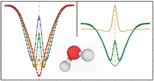The 71 newly observed lines, combined with further highly accurate literature transitions, allow the determination of the relative energies for all of the 59 rovibrational states up to J = 6 within the $(v_1{v}_2{v}_3)=(200)$ vibrational parent of ${\mathrm{H}}_2{}^{16}\mathrm{O}$, where J is the overall rotational quantum number and $v_1$, $v_2$, and $v_3$ are quantum numbers associated with the symmetric stretch, bend, and antisymmetric stretch normal modes, respectively. An experimental curiosity of this study is that for strong transitions an apparent signal inversion in the Lamb-dip spectra is observed; a novelty reserved to the NICE-OHMS technique.

GRAPHICAL ABSTRACT

Keywords:

• Water molecule
• vibrational band
• NICE-OHMS
• spectroscopic network
• saturation spectroscopy

1. Introduction

Water isotopologues, all of them asymmetric-top molecules, have been widely employed as test systems for modelling efforts in high-resolution and precision spectroscopy. The interest in water spectroscopy [1] is due partly to the fact that water spectra are involved in a huge number of important scientific and engineering applications, e.g. combustion, atmospheric sciences, and astronomy, either directly or indirectly (in the latter case the application requires the subtraction of water lines to reveal the lines of interest). Therefore, extensive line lists exist for at least nine water isotopologues [2–8].

For the main water isotopologue, ${\mathrm{H}}_2{}^{16}\mathrm{O}$, the related spectroscopic databases contain some 300,000 experimental rovibrational lines and some 20,000 empirical energy levels. Dr. Jean-Marie Flaud, to whom this paper is dedicated, has made significant contributions [9–32] to these spectroscopic data collections, providing thousands of measured line positions, line intensities, and collision parameters for a number of water isotopologues. Furthermore, the pioneering work of Flaud et al. [13] related to the conversion of measured transitions to empirical energy values provided one of the pillars of the MARVEL (Measured Active Rotational-Vibrational Energy Levels) protocol [33–35] and turned the attention of the Hungarian co-authors of this study toward the analysis and utilisation of spectroscopic networks [36].

The rovibrational energy levels of ${\mathrm{H}}_2{}^{16}\mathrm{O}$ are separated into two components, corresponding to the ortho and para nuclear-spin isomers. As of today, ortho–para transitions have not been detected for ${\mathrm{H}}_2{}^{16}\mathrm{O}$ due to their extremely low transition intensities [37]; thus, only relative energies can be determined from the measured lines. The relative energy of an ortho(para) state is defined as the difference between the absolute energy of this state and that of the lowest-energy ortho(para) state. In spectroscopy the absolute energy of the lowest para state $(v_1{v}_2{v}_3)J_{K_a,K_c}=(000)0_{0,0}$, is zero by definition, where $v_1$, $v_2$, and $v_3$ are the symmetric stretch, bend, and anti-symmetric stretch normal-mode quantum numbers, respectively, while $J_{K_a,K_c}$ stands for the asymmetric-top rotational quantum numbers [38]; thus, the relative para energies correspond to absolute energies. The most accurate empirical estimate for the absolute energy of the lowest ortho state, $(000)1_{0,1}$, is 23.79436122(25) cm${}^{-1}$ [39], enabling the accurate conversion of the relative ortho energies to absolute ones.

While all the experimental studies of Flaud and co-workers were based on Doppler-broadened spectroscopy, the advent of cavity-enhanced techniques has opened up a new territory, allowing experiments with much improved accuracy outside of the microwave spectral region. Such experiments in the near infra-red have already been carried out for ${\mathrm{H}}_2{}^{16}\mathrm{O}$, ${\mathrm{H}}_2{}^{17}\mathrm{O}$, and ${\mathrm{H}}_2{}^{18}\mathrm{O}$ [39–43]. The combination of ultrasensitive Noise-Immune Cavity Enhanced Optical Heterodyne Molecular Spectroscopy (NICE-OHMS) [44, 45] and the spectroscopic-network-assisted precision spectroscopy (SNAPS) procedure [39] has led to the derivation of a considerable number of ultraprecise absolute energies of ${\mathrm{H}}_2{}^{16}\mathrm{O}$ [39] and ${\mathrm{H}}_2{}^{18}\mathrm{O}$ [42] in the ground vibrational state.

In this study, 71 ultraprecise rovibrational lines of ${\mathrm{H}}_2{}^{16}\mathrm{O}$ are reported, observed with the NICE-OHMS technique in the 1.4 $\text{μ}$m region. Relying on the newly recorded transitions selected via the SNAPS scheme, as well as those of [39, 40, 46–48], accurate relative energies are deduced with an uncertainty of at most 15 kHz. Altogether 59 ultraprecise relative energies are determined this way for  the $(200)$ vibrational parent, forming a complete set up to J = 6. The newly derived relative energies allow the extension of an ultraprecise predicted line list of ${\mathrm{H}}_2{}^{16}\mathrm{O}$ [39], benefiting all those who require accurate spectroscopic information for their modelling efforts.

2. Methodological details

2.1. NICE-OHMS

NICE-OHMS [44, 45] is an absorption-based saturation-spectroscopy technique combining frequency modulation with cavity enhancement. A detailed description of our in-house NICE-OHMS spectrometer is given in [49], while the application of our setup to the study of water lines has been described in detail in [39, 42].

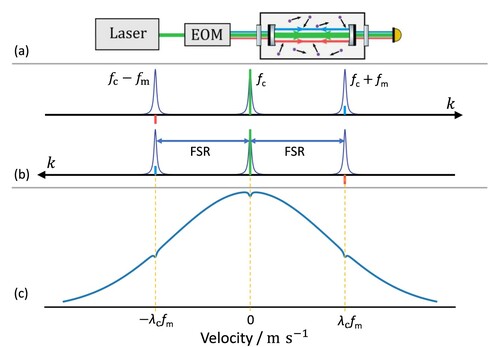
The technique of NICE-OHMS is based on the modulation of a laser, the carrier with frequency $f_{\mathrm{c}}$, to generate two opposite-phase sidebands with frequencies $f_{\mathrm{c}}\pm f_{\mathrm{m}}$ for heterodyne detection, where $f_{\mathrm{m}}$ is the modulation frequency (see Figure 1(a)). The in-phase sideband, that with frequency $f_{\mathrm{c}}+f_{\mathrm{m}}$, has the same phase as the carrier, while the other one with frequency $f_{\mathrm{c}}-f_{\mathrm{m}}$, named out-of-phase sideband, is shifted in its phase by 180${}^{\circ }$ with respect to the carrier. The three fields moving in both directions within the cavity must exactly match the resonant cavity modes, requiring $f_{\mathrm{m}}=\mathrm{FSR}$, where FSR is the free spectral range of the cavity (see Figure 1(b)). When $f_{\mathrm{c}}=f$ is set, where f is the central position of a molecular resonance, both counter-propagating carrier fields interact with the molecules flying perpendicularly. This interaction produces a hole burnt in the center of the axial velocity distribution and enables the observation of generic Doppler-free Lamb dips.

In addition to this generic Lamb dip, the two counter-propagating sidebands interact with molecules flying parallel to the beam and carrying a velocity of $\pm {\lambda }_{\mathrm{c}}{f}_{\mathrm{m}}$, where ${\lambda }_{\mathrm{c}}$ is the wavelength of the carrier. Due to the Doppler effect, molecules with these velocities perceive the sideband frequencies at f, leading to additional hole burning [50]. These holes appear in the axial velocity distribution at $\pm {\lambda }_{\mathrm{c}}{f}_{\mathrm{m}}$, forming two additional identical Lamb dips at $f_{\mathrm{c}}=f$ (see Figure 1(c)). All three Lamb dips are acquired simultaneously at $f_{\mathrm{c}}=f$, but the Lamb-dips generated by the sidebands are opposite in sign, as the out-of-phase sideband causes the sign to flip. Under most conditions the widths of the Lamb dips are nearly identical, leading only to a slight attenuation of the observed Lamp dip. However, in the case of strong resonances, the carrier-carrier saturation significantly broadens the Lamb dip. This broadening ensures sufficient contrast to observe the sideband-sideband Lamb dip separately, resulting in a notable double-dip profile.

Experimental constraints on the selection of target lines are imposed by the operating ranges of the diode laser, the frequency-comb laser, and the high-reflectivity mirrors. A further constraint is that the Lamb-dip spectra can be probed most efficiently within a limited range of intensities (${10}^{-26}$–${10}^{-21}$ cm molecule${}^{-1}$) and Einstein A-coefficients (${10}^{-4}$–${10}^2$ s${}^{-1}$).

Figure 1. Interaction among the multiple laser fields inside the cavity. Panel (a) shows the generation of the sidebands through the Electro Optic Modulator (EOM) with a modulation frequency $f_{\mathrm{m}}$. The EOM generates from an input field at frequency $f_{\mathrm{c}}$, the carrier, two sideband fields at frequencies $f_{\mathrm{c}}+f_{\mathrm{m}}$ and $f_{\mathrm{c}}-f_{\mathrm{m}}$. The thick green arrow represents the carrier field, at much higher power than the in-phase (blue) and out-of-phase (red) sidebands. The parameter $f_{\mathrm{m}}$ is set to the free spectral range (FSR), which is 305 MHz. Panel (b) illustrates the three fields coupled into three adjacent cavity modes and separated by the FSR. The matching cavity modes of the carrier, the in-phase sideband, and the out-of-phase sideband are denoted with green, blue, and red spikes, respectively. The two arrows labelled with k show the opposite propagation directions of the three bi-directionally propagating laser fields. Panel (c) exhibits the three distinctive holes burnt into the axial velocity distribution profile, all contributing to the observed lineshape. ${\lambda }_{\mathrm{c}}$ is the wavelength of the carrier.

2.2. SNAPS

The SNAPS procedure, built upon the theory of spectroscopic networks [36] and the Ritz principle [51], is well documented, see [39, 42]. Briefly, during the execution of SNAPS, one should (a) build paths and cycles (see Figure 2 of [42]) from highly-accurate ‘predetermined’ (literature) lines, as well as from target transitions satisfying the experimental constraints; (b) continue with recording the target lines; and (c) evaluate the spectroscopic information coded in the paths and cycles of the new and the predetermined transitions. The paths provide ultraprecise estimates for the energy differences and their uncertainties, while the cycles can be applied to test the internal accuracy of the newly resolved lines.

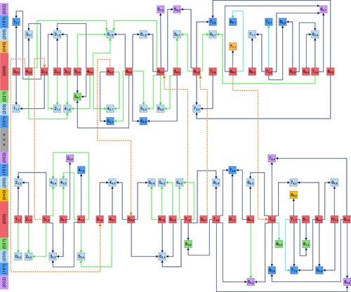
Figures 2 and 3 give an overview of all the ultraprecise lines observed for ortho- and para-${\mathrm{H}}_2{}^{16}\mathrm{O}$, respectively. The ‘light green’ transitions of Figures 2 and 3 are detected during this study, while all the other lines have been measured before [39, 40, 46–48], with a few kHz accuracy. In Figures 2 and 3, two poorly-connected subnetworks can be recognised within the ortho and para components. The $p^{+}$, $p^{-}$, $o^{+}$, and $o^{-}$ subnetworks correspond to the $(p^{″},q^{″})=(+1,+1)$, $(-1,+1)$, $(+1,-1)$, $(-1,-1)$ pairs, respectively, where $p^{″}=(-1{)}^{K_c^{″}}$ and $q^{″}=(-1{)}^{v_3^{″}+K_a^{″}+K_c^{″}}$, while $v_3^{″}$, $K_a^{″}$, and $K_c^{″}$ are lower-state quantum numbers. Despite the fact that the para ($q^{″}=+1$) component cannot be linked via experimental transitions with the ortho ($q^{″}=-1$) component, the $p^{+}/p^{-}$ and $o^{+}/o^{-}$ subnetworks are connected with pure rotational lines [46–48]. Considering only dipole-allowed, vibrational-state-altering lines, these subnetworks are fully decoupled from each other. Unlike in the case of ${\mathrm{H}}_2{}^{18}\mathrm{O}$ [42], only the p⁺ subnetwork of ${\mathrm{H}}_2{}^{16}\mathrm{O}$ is connected in itself, but the pure rotational lines make the ortho and para components entirely connected.

Figure 2. Pictorial representation of the precision lines observed for ortho-${\mathrm{H}}_2{}^{16}\mathrm{O}$. The rovibrational states are designated with $(v_1{v}_2{v}_3)J_{K_a,K_c}$, whereby $v_3+K_a+K_c$ is odd. The rovibrational lines correspond to $(v_1^{\prime }{v}_2^{\prime }{v}_3^{\prime })J_{K_a^{\prime },K_c^{\prime }}^{\prime }\leftarrow (v_1^{″}{v}_2^{″}{v}_3^{″})J_{K_a^{″},K_c^{″}}^{″}$, where ${}^{\prime }$ and ${}^{″}$ distinguish between the upper and lower states, respectively. Based on the even and odd parity of $K_c^{″}$, the near-infrared transitions can be divided into two subnetworks, $o^{+}$ and $o^{-}$, respectively, which are drawn separately. The $J_{K_a,K_c}$ rotational label is written out explicitly for each state in a circle, while the ($v_1{v}_2{v}_3$) vibrational labels [52] are indicated in the left-side colour legend. The vibrational states of this figure belong to the $P=0,$ 4, and 5 polyads, where $P=2v_1+v_2+2v_3$ is the polyad number. Transitions with light green arrows are results of the present study, while those with cyan, dark blue, grey, orange, and purple colours are taken from [39, 40, 46–48], respectively. Dashed arrows represent pure rotational lines linking the $o^{+}$ and $o^{-}$ subnetworks. The complete list of these ultraprecise transitions with their line centers and uncertainties are deposited in the Supplementary Material.

Figure 3. Pictorial representation of the precision lines observed for para-${\mathrm{H}}_2{}^{16}\mathrm{O}$. The specification of the rovibrational states and lines, as well as the formalism applied, is similar to that of Figure 2, with the difference that the para levels, identified with even $v_3+K_a+K_c$ values, are represented with squares. The NICE-OHMS transitions are organised into subnetworks $p^{+}$ and $p^{-}$, where the lines are characterised by even and odd $K_c^{″}$ values, respectively. The complete list of these ultraprecise transitions with their frequencies and uncertainties are deposited in the Supplementary Material.

3. Experimental results

3.1. Lineshapes of NICE-OHMS spectra

For the 71 ‘light green’ transitions shown in Figures 2 and 3, accurate line centers have been derived from the Lamb dips recorded during this study. The ultraprecise line positions and their individual uncertainties, representing 68 % confidence level, are given in Table 1.

Table 1. The complete list of the rovibrational transitions of ${\mathrm{H}}_2{}^{16}\mathrm{O}$ measured during this study, along with individual uncertainties.

No.	Assignment	Frequency (kHz)	No.	Assignment	Frequency (kHz)
1	$(101)4_{1,3}\leftarrow (000)5_{3,2}$	$\mathrm{210,106,545},991.7\pm 7.7$	37	$(200)4_{2,2}\leftarrow (000)3_{3,1}$	$\mathrm{216,467,935,097.0}\pm 4.9$
2	$(200)2_{2,1}\leftarrow (000)3_{3,0}$	$\mathrm{211,173,854,736.3}\pm 7.5$	38	$(200)6_{4,3}\leftarrow (000)7_{1,6}$	$\mathrm{216,533,504,194.3}\pm 5.1$
3	$(200)3_{0,3}\leftarrow (000)3_{3,0}$	$\mathrm{211,297,750,216.9}\pm 5.2$	39	$(200)2_{1,1}\leftarrow (000)2_{0,2}$	$\mathrm{216,543,604,990.8}\pm 7.7$
4	$(200)6_{1,6}\leftarrow (000)6_{2,5}$	$\mathrm{212,228,360,502.3}\pm 7.5$	40	$(200)6_{2,5}\leftarrow (000)5_{3,2}$	$\mathrm{216,584,789,651.7}\pm 7.7$
5	$(200)4_{3,1}\leftarrow (000)4_{4,0}$	$\mathrm{212,275,745,088.6}\pm 7.8$	41	$(200)6_{3,3}\leftarrow (000)5_{4,2}$	$\mathrm{216,713,868,387.2}\pm 5.3$
6	$(200)6_{4,3}\leftarrow (000)7_{3,4}$	$\mathrm{212,392,094,941.0}\pm 7.6$	42	$(200)4_{2,2}\leftarrow (000)4_{1,3}$	$\mathrm{216,759,402,341.3}\pm 7.5$
7	$(200)5_{3,3}\leftarrow (000)6_{2,4}$	$\mathrm{212,429,214,349.8}\pm 7.5$	43	$(200)3_{1,2}\leftarrow (000)3_{0,3}$	$\mathrm{216,816,255,011.5}\pm 8.0$
8	$(200)6_{0,6}\leftarrow (000)6_{1,5}$	$\mathrm{212,516,880,028.2}\pm 7.5$	44	$(200)5_{2,3}\leftarrow (000)5_{1,4}$	$\mathrm{216,845,549,472.7}\pm 7.6$
9	$(200)4_{2,3}\leftarrow (000)5_{1,4}$	$\mathrm{212,549,726,957.8}\pm 7.5$	45	$(200)3_{1,2}\leftarrow (000)2_{2,1}$	$\mathrm{216,872,016,984.5}\pm 7.7$
10	$(200)5_{1,5}\leftarrow (000)5_{2,4}$	$\mathrm{212,843,780,343.4}\pm 7.6$	46	$(200)6_{3,3}\leftarrow (000)6_{2,4}$	$\mathrm{216,933,944,189.3}\pm 7.5$
11	$(200)1_{1,0}\leftarrow (000)2_{2,1}$	$\mathrm{213,065,280,386.0}\pm 7.6$	47	$(200)5_{4,2}\leftarrow (000)6_{1,5}$	$\mathrm{217,091,029,773.4}\pm 13.8$
12	$(200)3_{0,3}\leftarrow (000)4_{1,4}$	$\mathrm{213,113,898,650.5}\pm 7.6$	48	$(200)5_{3,3}\leftarrow (000)6_{0,6}$	$\mathrm{217,108,282,261.0}\pm 7.5$
13	$(200)5_{0,5}\leftarrow (000)5_{1,4}$	$\mathrm{213,317,003,151.8}\pm 7.6$	49	$(200)4_{3,2}\leftarrow (000)5_{0,5}$	$\mathrm{217,135,374,647.8}\pm 7.6$
14	$(200)6_{5,1}\leftarrow (000)7_{4,4}$	$\mathrm{213,504,626,962.6}\pm 7.6$	50	$(200)4_{1,3}\leftarrow (000)4_{0,4}$	$\mathrm{217,221,204,437.3}\pm 7.5$
15	$(200)5_{4,2}\leftarrow (000)6_{3,3}$	$\mathrm{213,534,197,982.8}\pm 7.5$	51	$(200)3_{0,3}\leftarrow (000)2_{1,2}$	$\mathrm{217,471,142,188.6}\pm 8.0$
16	$(200)2_{0,2}\leftarrow (000)3_{1,3}$	$\mathrm{213,663,124,480.5}\pm 7.6$	52	$(200)4_{1,3}\leftarrow (000)3_{2,2}$	$\mathrm{217,693,417,582.6}\pm 7.6$
17	$(200)6_{0,6}\leftarrow (000)5_{3,3}$	$\mathrm{213,684,202,168.2}\pm 15.5$	53	$(200)4_{4,1}\leftarrow (000)5_{1,4}$	$\mathrm{217,831,529,702.9}\pm 7.8$
18	$(101)4_{1,3}\leftarrow (000)4_{3,2}$	$\mathrm{213,892,779,969.1}\pm 7.7$	54	$(200)6_{4,2}\leftarrow (000)6_{3,3}$	$\mathrm{217,840,321,863.3}\pm 7.5$
19	$(200)5_{4,1}\leftarrow (000)6_{3,4}$	$\mathrm{213,917,346,155.8}\pm 7.5$	55	$(200)4_{3,2}\leftarrow (000)4_{2,3}$	$\mathrm{217,884,424,690.3}\pm 7.5$
20	$(200)6_{6,1}\leftarrow (000)7_{5,2}$	$\mathrm{213,930,734,812.6}\pm 7.5$	56	$(200)4_{0,4}\leftarrow (000)3_{1,3}$	$\mathrm{218,048,663,367.3}\pm 7.5$
21	$(200)6_{6,0}\leftarrow (000)7_{5,3}$	$\mathrm{213,936,479,008.5}\pm 7.7$	57	$(002)6_{4,2}\leftarrow (000)6_{5,1}$	$\mathrm{218,094,331,523.0}\pm 7.5$
22	$(200)4_{0,4}\leftarrow (000)4_{1,3}$	$\mathrm{214,054,871,531.4}\pm 7.6$	58	$(200)5_{4,1}\leftarrow (000)5_{3,2}$	$\mathrm{218,119,436,295.0}\pm 7.7$
23	$(200)5_{5,1}\leftarrow (000)6_{4,2}$	$\mathrm{214,327,159,420.1}\pm 16.8$	59	$(200)4_{1,4}\leftarrow (000)3_{0,3}$	$\mathrm{218,281,318,913.5}\pm 7.9$
24	$(200)5_{5,0}\leftarrow (000)6_{4,3}$	$\mathrm{214,359,556,842.4}\pm 7.5$	60	$(200)4_{4,1}\leftarrow (000)4_{3,2}$	$\mathrm{218,339,397,004.6}\pm 8.1$
25	$(200)4_{1,3}\leftarrow (000)4_{2,2}$	$\mathrm{214,411,346,495.5}\pm 7.5$	61	$(200)6_{2,5}\leftarrow (000)6_{1,6}$	$\mathrm{218,430,303,230.1}\pm 7.5$
26	$(200)4_{4,1}\leftarrow (000)5_{3,2}$	$\mathrm{214,553,163,026.1}\pm 7.7$	62	$(200)5_{0,5}\leftarrow (000)4_{1,4}$	$\mathrm{218,551,953,037.4}\pm 7.5$
27	$(200)2_{1,1}\leftarrow (000)2_{2,0}$	$\mathrm{214,562,783,143.0}\pm 7.6$	63	$(200)6_{5,1}\leftarrow (000)6_{4,2}$	$\mathrm{218,600,010,890.1}\pm 7.9$
28	$(200)0_{0,0}\leftarrow (000)1_{1,1}$	$\mathrm{214,783,393,303.8}\pm 4.9$	64	$(200)5_{1,5}\leftarrow (000)4_{0,4}$	$\mathrm{218,664,430,158.9}\pm 7.6$
29	$(200)2_{0,2}\leftarrow (000)2_{1,1}$	$\mathrm{215,075,223,293.4}\pm 7.5$	65	$(200)5_{5,0}\leftarrow (000)5_{4,1}$	$\mathrm{218,748,027,171.1}\pm 7.8$
30	$(200)5_{2,3}\leftarrow (000)6_{1,6}$	$\mathrm{215,412,696,377.5}\pm 7.5$	66	$(200)5_{5,1}\leftarrow (000)5_{4,2}$	$\mathrm{218,754,067,492.0}\pm 7.5$
31	$(200)6_{1,6}\leftarrow (000)5_{2,3}$	$\mathrm{215,418,173,888.3}\pm 7.7$	67	$(200)6_{6,0}\leftarrow (000)6_{5,1}$	$\mathrm{219,063,350,040.7}\pm 7.6$
32	$(200)5_{1,5}\leftarrow (000)4_{2,2}$	$\mathrm{215,854,572,224.0}\pm 7.7$	68	$(200)6_{6,1}\leftarrow (000)6_{5,2}$	$\mathrm{219,064,282,101.9}\pm 7.6$
33	$(200)4_{2,3}\leftarrow (000)3_{3,0}$	$\mathrm{215,968,528,410.1}\pm 4.9$	69	$(200)5_{2,4}\leftarrow (000)4_{1,3}$	$\mathrm{219,622,319,934.8}\pm 7.6$
34	$(200)4_{1,4}\leftarrow (000)3_{2,1}$	$\mathrm{216,021,042,437.9}\pm 4.9$	70	$(200)6_{4,2}\leftarrow (000)7_{1,7}$	$\mathrm{220,090,855,818.2}\pm 8.4$
35	$(200)5_{2,4}\leftarrow (000)4_{3,1}$	$\mathrm{216,374,204,401.9}\pm 4.8$	71	$(200)4_{3,1}\leftarrow (000)4_{0,4}$	$\mathrm{220,252,665,298.9}\pm 7.6$
36	$(200)1_{1,0}\leftarrow (000)1_{0,1}$	$\mathrm{216,396,192,933.5}\pm 5.3$

In Figure 4, characteristic Lamb-dip spectra are shown for four distinct lines probed with our NICE-OHMS spectrometer. For the weaker transitions, see panels (a) and (c), an ordinary single-dip absorption feature can be observed. These Lamb-dip profiles, which are typical in saturation spectroscopy [53], have a full width at half maximum (FWHM) of ∼600 kHz. For the stronger transitions, connecting low-J levels, see panels (b) and (d), atypical, double-dip Lamb-dip profiles have been observed.

Figure 4. Spectral recordings of four Lamb-dip lines obtained in this study with their rovibrational assignments indicated. On panels (a,b) and (c,d), para- and ortho-${\mathrm{H}}_2{}^{16}\mathrm{O}$ transitions are depicted, respectively. Note that the double-dip line profiles, depicted in panels (b) and (d), arise when the underlying transitions have large Einstein-A coefficients.

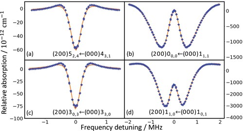
The signature of strong saturated lines in NICE-OHMS consists of three independent Lamb-dip contributions when the carrier frequency is tuned to $f_{\mathrm{c}}=f$ as described in Section 2.1. The interference of the three Lamb-dips yields a notable double-dip profile if their widths are significantly different. This is the case for strong water transitions, as the high-power carrier induces much higher power broadening in comparison to the weaker sidebands, allowing the detection of double-dip signals.

During the course of the experimental campaign, the characteristic Lamb-dip reversal was detected for lines with Einstein-A coefficients >0.1 s${}^{-1}$. Figure 5(a) exhibits a number of spectra for the $(200)0_{0,0}\leftarrow (000)1_{1,1}$ transition, demonstrating the enhancement of Lamb-dip reversion at increasing sideband powers, without any shift in the line center. As Figure 5(b) shows, the recorded signal can be fitted accurately by using a combination of two opposite sign fitting functions (i.e. first derivatives of dispersive Lorentzians [43]). Note that these double-dip line profiles, presented for the first time, occur exclusively in NICE-OHMS spectra and cannot be observed with other cavity-enhanced methods using only one intracavity laser field.

Figure 5. Spectral recordings of NICE-OHMS signals for the $(200)0_{0,0}\leftarrow (000)1_{1,1}$ line of ${\mathrm{H}}_2{}^{16}\mathrm{O}$. Panel (a) shows the spectral profile at various sideband (SB) powers [see the legend of panel (a)] and at fixed carrier power of 15 W. The dashed marker represents the position of the line center. Panel (b) illustrates the individual components of the double-dip spectra at a sideband power of 122 mW. The orange profile corresponds to the two coincident Lamb-dips, with a FWHM of 0.5 MHz, induced by the sideband fields. The blue profile of ordinary sign, with a FWHM of 2.4 MHz, is generated by the carrier. The combination of the orange and blue profiles leads to the recorded signal, denoted with a green curve.

3.2. Uncertainty quantification

The uncertainties of the transition frequencies displayed in Table 1 depend on several experimental effects arising mostly from homogeneous broadening mechanisms [53]. In this study, the following decomposition is applied to estimate the uncertainty of a measured frequency, δ: (1) $\delta =\sqrt{{\delta }_{\mathrm{stat}}^2+{\delta }_{\mathrm{day}}^2+{\delta }_{\mathrm{pow}}^2+{\delta }_{\mathrm{pres}}^2+{\delta }_{\mathrm{instr}}^2}.$(1) The statistical uncertainty, ${\delta }_{\mathrm{stat}}$, describes the reproducibility of the NICE-OHMS line positions. ${\delta }_{\mathrm{stat}}$ is approximated as the standard deviation of the transition frequencies derived from 3–4 scans. The day-to-day uncertainty, ${\delta }_{\mathrm{day}}$, is related to ${\delta }_{\mathrm{stat}}$, specifying the long-term reproducibility of the line centers and the stability of the NICE-OHMS setup. The spectra of some transitions were repeatedly recorded on 2–3 different days, yielding an average deviation of 2.5 kHz for these lines. This average deviation is used as ${\delta }_{\mathrm{day}}$ for each line probed. The uncertainty due to power-induced shifts, ${\delta }_{\mathrm{pow}}$, was diminishing, i.e. below 1 kHz, during the experiments. Therefore, a robust estimate of ${\delta }_{\mathrm{pow}}=0.5$ kHz is applied for all transitions.

If the vapour pressure is not negligible in the sample cell, the pressure-shift uncertainty, ${\delta }_{\mathrm{pres}}$, is significant. For lines $(200)0_{0,0}\leftarrow (000)1_{1,1}$ and $(200)4_{1,4}\leftarrow (000)3_{2,1}$, the pressure-shift effects were explicitly considered by recording spectra over a range of pressure values and extrapolating the transition frequencies to zero pressure and fitting a linear model, $f=Cp+f_{\mathrm{vac}}$, where f and $f_{\mathrm{vac}}$ are the transition frequencies at pressure p and in vacuum, respectively, and C denotes the pressure-shift coefficient (slope). The C coefficients determined in this study are +17.3  kHz Pa${}^{-1}$ [$(200)0_{0,0}\leftarrow (000)1_{1,1}$] and +4.5 kHz Pa${}^{-1}$ [$(200)4_{1,4}\leftarrow (000)3_{2,1}$]. Since the C values found in this study and in [39] fall into the range of $[-21,+22]$ kHz Pa${}^{-1}$, ${\delta }_{\mathrm{pres}}=C_{\mathrm{eff}}p$ is set for each new line, where $C_{\mathrm{eff}}=20$ kHz Pa${}^{-1}$, and p is the measurement pressure for the particular line. Since the pressure range applied is 0.01–0.2 Pa, ${\delta }_{\mathrm{pres}}$ corresponds to 0.2–4 kHz.

The ${\delta }_{\mathrm{instr}}$ factor is included in the uncertainty budget to describe the small frequency shifts due to an unbalanced Pound–Drever–Hall ‘lock’ causing slight asymmetries in the line profiles leading to fitting errors [54]. For nine selected transitions, this unbalance in the lock was corrected, revealing an average shift of ≈7 kHz. For these nine lines, ${\delta }_{\mathrm{instr}}=4$ kHz was chosen, while for all the other transitions ${\delta }_{\mathrm{instr}}=7$ kHz was adopted. For all the lines recorded in the present study, the values of the five uncertainty factors are listed in the Supplementary Material.

As an independent confirmation of the frequency uncertainties and the rovibrational assignments, all but one of the new NICE-OHMS lines were enclosed into cycles of different lengths. The only exception is the $(200)0_{0,0}\leftarrow (000)1_{1,1}$ line, whose upper state is not attainable from another pure rotational level through dipole-allowed transitions in our wavenumber range. To accelerate the experimental part of the cycle-based verification, the lines of the intermediate dataset were used to refine the initial positions via the Λ-correction scheme [42]. Furthermore, only two scans were performed instead of the usual four for those lines whose upper states were already determined accurately from other transitions. A subset of cycles, which helped to recognise an accidental mistake during the experiments, is plotted in Figure 6, while a collection of basic cycles [55, 56], whose discrepancy is typically 10 kHz or better for the final dataset, are placed in the Supplementary Material.

Figure 6. Typical short cycles formed during the SNAPS analysis. For the definitions of the colour codes and the elements of this figure, see the captions to Figures 2 and 3. The values on the arrows are transition frequencies in kHz, with the uncertainties of the last few digits given in parentheses. Combining any pairs of the three green lines with the blue transitions, three cycles of length 4, 6, and 8 are obtained. The brown frequency contains an additional error of +113.8 kHz, which was due to a miscalibration made during the measurement campaign. Using this erroneous frequency, the discrepancy [39] of the 6-membered cycle became an unacceptably large value of 119.4(121) kHz. Assuming that the blue transitions are correct, the green transition frequency was measured to decide which of the other two green lines causes the large discrepancy. Using the green frequency, the discrepancies of the 4- and 8-membered cycles were 111.5(126) and 7.9(138) kHz, respectively. The small discrepancy of the 8-membered cycle suggested that the brown frequency missing from this cycle should be responsible for the significant discrepancies of the other two cycles. After remeasuring the brown frequency, a new line center of 218 664 430 158.9 kHz was obtained. With this new line center, the discrepancies of the 4- and 6-membered cycles have been reduced to fairly small values, 2.3(126) and 5.6(121) kHz, respectively.

4. SNAPS-based results

4.1. Highly accurate relative energies

From the connected sets of the kHz-accuracy ortho and para transitions displayed in Figures 2 and 3, ultraprecise relative energies can be determined for the underlying ortho and para states, respectively. The relative energy of a particular ortho/para state is estimated here by constructing a lowest-uncertainty path from $(000)1_{0,1}$/$(000)0_{0,0}$ to the desired state and employing the Ritz principle in a successive way [39]. If the ortho and para components are linked with an artificial transition $(000)1_{0,1}\leftarrow (000)0_{0,0}$, whose wavenumber is set to 23.794 361 22(25) cm${}^{-1}$ [39], then one can also form paths from para states to their ortho siblings.

As an example, a path from $(200)0_{0,0}$ to $(200)1_{0,1}$ is presented in Figure 7. This path is capable of providing energy differences for any pair of the underlying states with definitive uncertainties. By taking the subpath from $(000)0_{0,0}$ to $(200)0_{0,0}$, the $(200)0_{0,0}$ energy, which is actually the vibrational band origin (VBO) of the $(200)$ vibrational parent, can be calculated as 7201.53995061(29) cm${}^{-1}$. This datum is nearly 1000 times more accurate than the W2020 estimate of 7201.54000(45) cm${}^{-1}$ [8]. Based on the lines of Figure 7, the energy difference of the ortho $(200)1_{0,1}$ and para $(200)0_{0,0}$ states, ${ϵ}^{(200)}$, is 23.04064642(39) cm${}^{-1}$, which is much lower than its counterpart in the ground vibrational state, ${ϵ}^{(000)}=23.79436122(25)$ cm${}^{-1}$ [39]. To understand the change $\mathrm{\Delta }ϵ={ϵ}^{(000)}-{ϵ}^{(200)}$, recall that ${ϵ}^{(v_1{v}_2{v}_3)}$ is the ‘rotational energy’ of the $(v_1{v}_2{v}_3)1_{0,1}$ level within the normal-mode and rigid-rotor approximations. Then, ${ϵ}^{(v_1{v}_2{v}_3)}$ can be given as the sum of the two smallest effective rotational constants: ${ϵ}^{(v_1{v}_2{v}_3)}\approx B^{(v_1{v}_2{v}_3)}+C^{(v_1{v}_2{v}_3)}$. In the case of ${\mathrm{H}}_2{}^{16}\mathrm{O}$,  (2) $\begin{array}{rl}\mathrm{\Delta }ϵ& \approx B^{(000)}-B^{(200)}+C^{(000)}-C^{(200)}\\ & \approx 14.51-14.17+9.29-8.95=0.68{\mathrm{cm}}^{-1},\end{array}$(2) where the effective rotational constants are taken from [57]. This simple estimate is in good agreement with the SNAPS-based determination of 0.75371480(29) cm${}^{-1}$.

Relying on the lines of Figures 2 and 3, ultraprecise relative energies are derived, via the SNAPS scheme, for 192 energy levels. Of these states, 59 lie on the $(200)$ band and form a complete set up to J = 6. The relative energies of the 59 states, among which 32 have not been investigated in previous Lamb-dip studies [39, 40], are displayed, with individual uncertainties, in Table 2. The complete list of the 192 relative rovibrational energies is given in the Supplementary Material.

Figure 7. Path from the $(200)0_{0,0}$ (para) state to the $(200)1_{0,1}$ (ortho) state. The colour codes and the elements of the figure are explained in the captions to Figures 2 and 3, except the red dash-dotted line, which symbolises the calculated energy difference between the lowest ortho and para states, taken from [39]. The values on the arrows are transition wavenumbers in cm${}^{-1}$, with the uncertainties of the last few digits given in parentheses. Utilizing the Ritz principle in a successive form and exploiting the law of uncertainty propagation (see also [39]), the $(200)1_{0,1}-(200)0_{0,0}$ energy difference is estimated to be 23.040 646 42(39) cm${}^{-1}$. Note that from the subpaths of this path one can derive absolute energies for all the rovibrational states displayed in the figure.

Table 2. Ultraprecise relative energies in the $(200)$ vibrational band of ${\mathrm{H}}_2{}^{16}{\mathrm{O}}^{\mathrm{a}}$

Assignment (para)	Rel. energy (para) (cm${}^{-1}$)	Assignment (ortho)	Rel. energy (ortho) (cm${}^{-1}$)
$(200)0_{0,0}$	7201.53995061(29)	$(200)1_{0,1}$	7200.786235810(61)
$(200)1_{1,1}$	7236.80750451(14)	$(200)1_{1,0}$	7218.20003002(18)
$(200)2_{0,2}$	7269.31316664(29)	$(200)2_{1,2}$	7253.893683916(53)
$(200)2_{1,1}$	7293.20798308(29)	$(200)2_{2,1}$	7305.625797494(71)
$(200)2_{2,0}$	7331.62273401(16)	$(200)3_{0,3}$	7309.75850566(24)
$(200)3_{1,3}$	7338.25106968(14)	$(200)3_{1,2}$	7345.17909462(27)
$(200)3_{2,2}$	7398.40716108(23)	$(200)3_{2,1}$	7381.44363884(15)
$(200)3_{3,1}$	7472.95224315(18)	$(200)3_{3,0}$	7449.26681703(12)
$(200)4_{0,4}$	7415.59899771(29)	$(200)4_{1,4}$	7394.04836537(27)
$(200)4_{1,3}$	7467.77221388(30)	$(200)4_{2,3}$	7465.55889585(23)
$(200)4_{2,2}$	7505.81243506(33)	$(200)4_{3,2}$	7544.41002417(30)
$(200)4_{3,1}$	7568.89086382(30)	$(200)4_{4,1}$	7641.74087077(32)
$(200)4_{4,0}$	7665.57141588(25)	$(200)5_{0,5}$	7491.15247461(33)
$(200)5_{1,5}$	7515.91304208(30)	$(200)5_{1,4}$	7563.59182176(19)
$(200)5_{2,4}$	7601.30908677(34)	$(200)5_{2,3}$	7608.85211103(33)
$(200)5_{3,3}$	7688.64936255(35)	$(200)5_{3,2}$	7666.63979709(26)
$(200)5_{4,2}$	7784.28307110(41)	$(200)5_{4,1}$	7760.69894239(32)
$(200)5_{5,1}$	7906.96469276(42)	$(200)5_{5,0}$	7883.19559200(38)
$(200)6_{0,6}$	7631.70585896(41)	$(200)6_{1,6}$	7608.29313870(33)
$(200)6_{1,5}$	7725.44885815(25)	$(200)6_{2,5}$	7709.50864049(32)
$(200)6_{2,4}$	7784.02966286(27)	$(200)6_{3,4}$	7797.89506440(28)
$(200)6_{3,3}$	7838.91097588(36)	$(200)6_{4,3}$	7903.19993741(32)
$(200)6_{4,2}$	7927.91990288(40)	$(200)6_{5,2}$	8025.53121847(29)
$(200)6_{5,1}$	8049.49167620(44)	$(200)6_{6,1}$	8172.00229382(45)
$(200)6_{6,0}$	8195.79946638(41)	$(200)7_{2,5}$	7933.87434422(29)
$(200)7_{3,5}$	7985.28524726(37)	$(200)7_{6,1}$	8338.64298556(38)
$(200)7_{6,2}$	8362.40069771(34)	$(200)8_{6,3}$	8528.91446581(40)
$(200)7_{7,1}$	8530.40686109(40)	$(200)9_{3,6}$	8417.78773038(34)
$(200)8_{0,8}$	7917.72240604(29)
$(200)8_{3,5}$	8216.20356896(39)
$(200)9_{4,6}$	8482.46674719(37)

${}^{\mathrm{a}}$The relative energy is zero for the lowest ortho and para states. The uncertainties of the last few digits, related to 68% confidence level, are displayed in parentheses. The boldface entries are results of this study, all the other values are taken from [39]. For ortho-${\mathrm{H}}_2{}^{16}\mathrm{O}$, the formulas $E=$ $e+E_0$ and $u_E=\sqrt{u_e^2+u_{E_0}^2}$ can be used to derive absolute energies, where $E_0=23.79436122$ cm${}^{-1}$ is the absolute energy of the lowest ortho state [39] with an uncertainty of $u_{E_0}=2.5\times {10}^{-7}$ cm${}^{-1}$, and e and E are the relative and absolute energies of a given state with uncertainties $u_e$ and $u_E$, respectively.

4.2. Ultrahigh-accuracy predicted line list

Utilizing the relative SNAPS energies deduced from the lines of Figures 2 and 3, an ultraprecise predicted line list, satisfying one-photon, electric-dipole selection rules, has been compiled (for further details  about the generation of the line list, see Supplementary Note 6 of [39]). In the line list, the SNAPS wavenumbers, which are typically 100–1000 times more accurate than the previous line positions, are augmented with intensities determined from the Einstein-A coefficients of [58]. The complete line list, corresponding to the ranges of 0–1005 and 6200–8110 cm${}^{-1}$, is available in the Supplementary Material (see also Figure 8).

Our extended SNAPS-predicted line list contain 1743 transitions, including 524 extra entries in comparison to that of [39]. Of the 1743 lines, 983 are characterised with an intensity larger than $1\times {10}^{-26}$ cm molecule${}^{-1}$. These 983 entries, out of which 207 are results of the present study, may serve as calibration standards for high-resolution studies (e.g. in atmospheric spectroscopy). The predicted line list contains 21 closely-spaced ortho-para doublets with intensities of at least $1\times {10}^{-26}$ cm molecule${}^{-1}$ for the more intense member of each line pair. The separation of such a doublet is smaller than the Doppler FWHM at room temperature, that is $<0.02$ cm${}^{-1}$ in the 6200–8110 cm${}^{-1}$ region. Resolving these line pairs in room-temperature Doppler-broadened measurements is difficult, if possible at all.

Figure 8. Illustration of the ultrahigh-accuracy predicted line list of ${\mathrm{H}}_2{}^{16}\mathrm{O}$ assembled during this study. The wavenumbers are estimated from the SNAPS-based relative energies, while the one-photon, dipole-allowed intensities are deduced from the Einstein-A coefficients of [58]. The green diamonds designate the results of this study, while the blue squares represent estimates of [39]. Although the direct experimental lines used in the derivation of the relative energies are restricted to the regions 0–20 and 7000–7350 cm${}^{-1}$, the predicted transitions extend between 0–1005 and 6200–8110 cm${}^{-1}$. The points located in the upper left, lower left, and upper right quadrants correspond to $P^{\prime }-P^{″}=0-0$, 4−4, and 4−0, transitions, respectively, where $P^{\prime }$ and $P^{″}$ are the polyad numbers of the upper and lower states, respectively.

5. Conclusions

A saturation spectroscopic technique, the Noise-Immune Cavity Enhanced Optical Heterodyne Molecular Spectroscopy (NICE-OHMS), is employed to accurately measure rovibrational lines of ${\mathrm{H}}_2{}^{16}\mathrm{O}$ in the 1.4 $\text{μ}$m wavelength region. The observed lines are selected based on the scheme called spectroscopic-network-assisted precision spectroscopy (SNAPS) to form a complete set of ultraprecise relative energies within the $(v_1{v}_2{v}_3)=(200)$ band of ${\mathrm{H}}_2{}^{16}\mathrm{O}$ up to $J\le 6$, where J is the overall rotational quantum number and $v_1$, $v_2$, and $v_3$ are quantum numbers associated with the symmetric stretch, bend, and antisymmetric stretch normal modes, respectively. The typical accuracy achieved for the relative energies is $3\times {10}^{-7}$ cm${}^{-1}$. Since most previous determinations of the $(200)$ relative energies were obtained from Doppler-limited spectroscopy, the present values represent an improvement in accuracy of 2−3 orders of magnitude. Unlike in our previous studies [39, 42], focussing on the ground vibrational state of ${\mathrm{H}}_2{}^{16}\mathrm{O}$ and ${\mathrm{H}}_2{}^{18}\mathrm{O}$, no fitting of an effective Hamiltonian (EH) was attempted to the ultraprecise relative energies of the $(200)$ vibrational parent , part of the P = 4 polyad, where $P=2v_1+v_2+2v_3$ is the polyad number. As the published EH fits [59–61] prove, these models of strongly interacting states are unable to reproduce the accuracy of the Doppler-broadened P = 4 dataset, which is a few times ${10}^{-3}$ cm${}^{-1}$, not even after invoking a large number of parameters. The accuracy issue would be even more pronounced for the ultraprecise measurements of the present study.

A curiosity related to the NICE-OHMS measurements performed is that for relatively strong, low-J transitions an interesting signal inversion in their Lamb-dip spectra was observed. This phenomenon, reported for the first time, can be understood as the interference of strong saturation signals from the carrier frequency, leading to broadening of the generic Lamb dip, and the saturation signals originating from the much weaker sidebands, typically used in NICE-OHMS, one of which is out-of-phase leading to an inverted sign for the signal.

The 71 newly measured lines, forming a carefully designed spectroscopic network with the ultraprecise transitions of previous papers [39, 40, 46–48], allow a highly accurate determination of the $(200)1_{0,1}$–$(200)0_{0,0}$ energy difference, which is 23.040646421(39) cm${}^{-1}$. A similarly accurate estimate, 7201.53995061(29) cm${}^{-1}$, is obtained for the vibrational band origin (VBO) of the $(200)$ state, providing the most accurate VBO of ${\mathrm{H}}_2{}^{16}\mathrm{O}$. In comparison, the best previous estimate for this VBO, that in the W2020 dataset [7], is 7201.54000(45) cm${}^{-1}$.

The empirical line list based upon the relative energies determined in this and a previous NICE-OHMS [39] study of ${\mathrm{H}}_2{}^{16}\mathrm{O}$ consists of 1743 transitions. Out of the 1743 transitions, 983 are characterised with electric-dipole-allowed intensities larger than $1\times {10}^{-26}$ cm molecule${}^{-1}$; thus, they are relevant to a number of applications, including atmospheric modelling.

Disclosure statement

No potential conflict of interest was reported by the author(s).

Additional information

Funding

The research described has received funding from the European Commission (LASERLAB-EUROPE) [grant number 654148], a European Union's Horizon 2020 research and innovation programme. The work performed in Budapest received support from the National Research, Development and Innovation Office (NKFIH) [grant number K138293]. WU acknowledges the European Research Council for an ERC Advanced Grant [grant number 670168]. Further support was obtained from the Nederlandse Organisatie voor Wetenschappelijk Onderzoek (NWO) program (16MYSTP) and from the NWO Dutch Astrochemistry Network.

References

- P.F. Bernath, Phys. Chem. Chem. Phys. 4, 1501–1509 (2002). doi:10.1039/b200372d
- I.E. Gordon, L.S. Rothman, C. Hill, R.V. Kochanov, Y. Tan, P.F. Bernath, M. Birk, V. Boudon, A. Campargue, K.V. Chance, B.J. Drouin, J.M. Flaud, R.R. Gamache, J.T. Hodges, D. Jacquemart, V.I. Perevalov, A. Perrin, K.P. Shine, M.A.H. Smith, J. Tennyson, G.C. Toon, H. Tran, V.G. Tyuterev, A. Barbe, A.G. Császár, V.M. Devi, T. Furtenbacher, J.J. Harrison, J.M. Hartmann, A. Jolly, T.J. Johnson, T. Karman, I. Kleiner, A.A. Kyuberis, J. Loos, O.M. Lyulin, S.T. Massie, S.N. Mikhailenko, N. Moazzen-Ahmadi, H.S.P. Müller, O.V. Naumenko, A.V. Nikitin, O.L. Polyansky, M. Rey, M. Rotger, S.W. Sharpe, K. Sung, E. Starikova, S.A. Tashkun, J.V. Auwera, G. Wagner, J. Wilzewski, P. Wcisło, S. Yu and E.J. Zak, J. Quant. Spectrosc. Radiat. Transf. 203, 3–69 (2017). doi:10.1016/j.jqsrt.2017.06.038
- I.E. Gordon, L.S. Rothman, R.J. Hargreaves, R. Hashemi, E.V. Karlovets, F.M. Skinner, E.K. Conway, C. Hill, R.V. Kochanova, Y. Tana, P. Wcislo, A.A. Finenko, K. Nelson, P.F. Bernath, M. Birk, V. Boudon, A. Campargue, K.V. Chance, A. Coustenis, B.J. Drouin, J. Flaud, R.R. Gamache, J.T. Hodges, D. Jacquemart, E.J. Mlawer, A.V. Nikitin, V.I. Perevalov, M. Rotger, K.P. Shines, J. Tennyson, G.C. Toon, H. Tran, V.G. Tyuterev, E.M. Adkins, A. Baker, A. Barber, E. Canev, A.G. Császár, O. Egorov, A.J. Fleisher, A. Foltynowicz, T. Furtenbacher, J.J. Harrison, J. Hartmann, V. Horneman, X. Huang, T. Karman, J. Karnsa, S. Kassi, I. Kleiner, V. Kofman, F. Kwabia-Tchana, T.J. Lee, D.A. Longo, A.A. Lukashevskaya, O.M. Lyulin, V.Y. Makhneva, S.T. Massie, M. Melosso, S.N. Mikhailenko, D. Mondelain, H.S.P. Müller, O.V. Naumenko, A. Perrin, O.L. Polyansky, E. Raddaoui, P.L. Rastonah, Z.D. Reed, M. Rey, C. Richard, R. Tóbiás, I. Sadieky, D.W. Schwenke, E. Starikova, K. Sung, F. Tamassia, S.A. Tashkun, J.V. Auwera, A.A. Vigasina, G.L. Villanueva, B. Vispoel, G. Wagner and S.N. Yurchenko, J. Quant. Spectrosc. Radiat. Transf. 276, 107949 (2022). doi:10.1016/j.jqsrt.2021.107949.
- N. Jacquinet-Husson, R. Armante, N.A. Scott, A. Chedin, L. Crepeau, C. Boutammine, A. Bouhdaoui, C. Crevoisier, V. Capelle, C. Boonne, N. Poulet-Crovisier, A. Barbe, D.C. Benner, V. Boudon, L.R. Brown, J. Buldyreva, A. Campargue, L.H. Coudert, V.M. Devi, M.J. Down, B.J. Drouin, A. Fayt, C. Fittschen, J.M. Flaud, R.R. Gamache, J.J. Harrison, C. Hill, O. Hodnebrog, S.M. Hu, D. Jacquemart, A. Jolly, E. Jimenez, N.N. Lavrentieva, A.W. Liu, L. Lodi, O.M. Lyulin, S.T. Massie, S. Mikhailenko, H.S.P. Mueller, O.V. Naumenko, A. Nikitin, C.J. Nielsen, J. Orphal, V.I. Perevalov, A. Perrin, E. Polovtseva, A. Predoi-Cross, M. Rotger, A.A. Ruth, S.S. Yu, K. Sung, S.A. Tashkun, J. Tennyson, V.I.G. Tyuterev, J.V. Auwera, B.A. Voronin and A. Makie, J. Mol. Spectrosc. 327, 31–72 (2016). doi:10.1016/j.jms.2016.06.007
- O.L. Polyansky, A.A. Kyuberis, L. Lodi, J. Tennyson, R.I. Ovsyannikov and N. Zobov, Mon. Not. R. Astron. Soc. 466, 1363–1371 (2017). doi:10.1093/mnras/stw3125
- O.L. Polyansky, A.A. Kyuberis, N.F. Zobov, J. Tennyson, S.N. Yurchenko and L. Lodi, Mon. Not. R. Astron. Soc. 480, 2597–2608 (2018). doi:10.1093/mnras/sty1877
- T. Furtenbacher, R. Tóbiás, J. Tennyson, O.L. Polyansky and A.G. Császár, J. Phys. Chem. Ref. Data 49, 033101 (2020). doi:10.1063/5.0008253
- T. Furtenbacher, R. Tóbiás, J. Tennyson, O.L. Polyansky, A.A. Kyuberis, R.I. Ovsyannikov, N.F. Zobov and A.G. Császár, J. Phys. Chem. Ref. Data 49, 043103 (2020). doi:10.1063/5.0030680
- J.M. Flaud, C. Camy-Peyret and A. Valentin, J. Phys (Paris) 33, 741–747 (1972). doi:10.1051/jphys:01972003308-9074100
- C. Camy-Peyret, J.M. Flaud, G. Guelachvili and C. Amiot, Mol. Phys. 26, 825–855 (1973). doi:10.1080/00268977300102131
- J.M. Flaud and C. Camy-Peyret, Mol. Phys. 26, 811–823 (1973). doi:10.1080/00268977300102121
- J.M. Flaud and C. Camy-Peyret, J. Mol. Spectrosc. 55, 278–310 (1975). doi:10.1016/0022-2852(75)90270-2
- J.M. Flaud, C. Camy-Peyret and J.P. Maillard, Mol. Phys. 32, 499–521 (1976). doi:10.1080/00268977600103251
- J.M. Flaud, C. Camy-Peyret, J.P. Maillard and G. Guelachvili, J. Mol. Spectrosc. 65, 219–228 (1977). doi:10.1016/0022-2852(77)90189-8
- J.M. Flaud, C. Camy-Peyret, J.P. Maillard and G. Guelachvili, Mol. Phys. 34, 413–426 (1977). doi:10.1080/00268977700101811
- J.M. Flaud, C. Camy-Peyret, K.N. Rao, D.W. Chen and Y.S. Hoh, J. Mol. Spectrosc. 75, 339–362 (1979). doi:10.1016/0022-2852(79)90081-X
- C. Camy-Peyret, J.M. Flaud and J.P. Maillard, J. Phys. Lett. (Paris) 41, 23–26 (1980). doi:10.1051/jphyslet:0198000410202300
- J.M. Flaud, C. Camy-Peyret and R.A. Toth, Water Vapour Line Parameters from Microwave to Medium Infrared (Pergamon, Oxford, 1981).
- A.S. Pine, M.J. Coulombe, C. Camy-Peyret and J.M. Flaud, J. Phys. Chem. Ref. Data 12, 413–465 (1983). doi:10.1063/1.555689
- C. Camy-Peyret, J.M. Flaud, J.Y. Mandin, J.P. Chevillard, J. Brault, D.A. Ramsay, M. Vervloet and J. Chauville, J. Mol. Spectrosc. 113, 208–228 (1985). doi:10.1016/0022-2852(85)90131-6
- J.Y. Mandin, J.P. Chevillard, C. Camy-Peyret and J.M. Flaud, J. Mol. Spectrosc. 118, 96–102 (1986). doi:10.1016/0022-2852(86)90227-4
- J.Y. Mandin, J.P. Chevillard, C. Camy-Peyret and J.M. Flaud, J. Mol. Spectrosc. 116, 167–190 (1986). doi:10.1016/0022-2852(86)90261-4
- J.P. Chevillard, J.Y. Mandin, J.M. Flaud and C. Camy-Peyret, Can. J. Phys. 65, 777–789 (1987). doi:10.1139/p87-114
- J.Y. Mandin, J.P. Chevillard, J.M. Flaud and C. Camy-Peyret, Can. J. Phys. 66, 997–1011 (1988). doi:10.1139/p88-162
- J.P. Chevillard, J.Y. Mandin, J.M. Flaud and C. Camy-Peyret, Can. J. Phys. 67, 1065–1084 (1989). doi:10.1139/p89-186
- V. Dana, J.Y. Mandin, C. Camy-Peyret, J.M. Flaud and L.S. Rothman, Appl. Opt. 31, 1179–1184 (1992). doi:10.1364/AO.31.001179
- J.Y. Mandin, V. Dana, C. Camy-Peyret and J.M. Flaud, J. Mol. Spectrosc. 152, 179–184 (1992). doi:10.1016/0022-2852(92)90128-B
- J.M. Flaud, C. Camy-Peyret, A. Bykov, O. Naumenko, T. Petrova, A. Scherbakov and L. Sinitsa, J. Mol. Spectrosc. 183, 300–309 (1997). doi:10.1006/jmsp.1997.7275
- J.M. Flaud, C. Camy-Peyret, A. Bykov, O. Naumenko, T. Petrova, A. Scherbakov and L. Sinitsa, J. Mol. Spectrosc. 185, 211–221 (1997). doi:10.1006/jmsp.1997.7377
- C. Camy-Peyret, J.M. Flaud, J.Y. Mandin, A. Bykov, O. Naumenko, L. Sinitsa and B. Voronin, J. Quant. Spectrosc. Radiat. Transf. 61, 795–812 (1999). doi:10.1016/S0022-4073(98)00068-5
- A. Bykov, O. Naumenko, L. Sinitsa, B. Voronin, J.M. Flaud, C. Camy-Peyret and R.A. Lanquetin, J. Mol. Spectrosc. 205, 1–8 (2001). doi:10.1006/jmsp.2000.8231
- S.N. Mikhailenko, V.G. Tyuterev, V.I. Starikov, K.K. Albert, B.P. Winnewisser, M. Winnewisser, G. Mellau, C. Camy-Peyret, R. Lanquetin, J.M. Flaud and J.W. Brault, J. Mol. Spectrosc. 213, 91–121 (2002). doi:10.1006/jmsp.2002.8558
- T. Furtenbacher, A.G. Császár and J. Tennyson, J. Mol. Spectrosc. 245, 115–125 (2007). doi:10.1016/j.jms.2007.07.005
- T. Furtenbacher and A.G. Császár, J. Quant. Spectrosc. Radiat. Transf. 113, 929–935 (2012). doi:10.1016/j.jqsrt.2012.01.005
- R. Tóbiás, T. Furtenbacher, J. Tennyson and A.G. Császár, Phys. Chem. Chem. Phys.21, 3473–3495 (2019). doi:10.1039/C8CP05169K
- A.G. Császár and T. Furtenbacher, J. Mol. Spectrosc. 266, 99–103 (2011). doi:10.1016/j.jms.2011.03.031
- A. Miani and J. Tennyson, J. Chem. Phys. 120, 2732–2739 (2004). doi:10.1063/1.1633261
- H.W. Kroto, Molecular Rotation Spectra (Dover, New York, 1992).
- R. Tóbiás, T. Furtenbacher, I. Simkó, A.G. Császár, M.L. Diouf, F.M.J. Cozijn, J.M.A. Staa, E.J. Salumbides and W. Ubachs, Nat. Commun. 11, 1708 (2020). doi:10.1038/s41467-020-15430-6
- S. Kassi, T. Stoltmann, M. Casado, M. Daeron and A. Campargue, J. Chem. Phys. 148, 054201 (2018). doi:10.1063/1.5010957
- J. Chen, T.P. Hua, L.G. Tao, Y. Sun, A.W. Liu and S.M. Hu, J. Quant. Spectrosc. Radiat. Transf.205, 91–95 (2018). doi:10.1016/j.jqsrt.2017.10.009
- M.L. Diouf, R. Tóbiás, I. Simkó, F.M.J. Cozijn, E.J. Salumbides, W. Ubachs and A.G. Császár, J. Phys. Chem. Ref. Data 50, 023106 (2021). doi:10.1063/5.0052744
- M. Melosso, M.L. Diouf, L. Bizzocchi, M.E. Harding, F.M.J. Cozijn, C. Puzzarini and W. Ubachs, J. Phys. Chem. A 125, 7884–7890 (2021). doi:10.1021/acs.jpca.1c05681
- L.S. Ma, J. Ye, P. Dubé and J.L. Hall, J. Opt. Soc. Am. B 16, 2255–2268 (1999). doi:10.1364/JOSAB.16.002255
- A. Foltynowicz, F.M. Schmidt, W. Ma and O. Axner, Appl. Phys. B 92, 313–326 (2008). doi:10.1007/s00340-008-3126-z
- S.G. Kukolich, J. Chem. Phys. 50, 3751–3755 (1969). doi:10.1063/1.1671623
- G.Y. Golubiatnikov, V.N. Markov, A. Guarnieri and R. Knochel, J. Mol. Spectrosc. 240, 251–254 (2006). doi:10.1016/j.jms.2006.09.012
- G. Cazzoli, C. Puzzarini, M.E. Harding and J. Gauss, Chem. Phys. Lett. 473, 21–25 (2009). doi:10.1016/j.cplett.2009.03.045
- F.M.J. Cozijn, P. Dupré, E.J. Salumbides, K.S.E. Eikema and W. Ubachs, Phys. Rev. Lett. 120, 153002 (2018). doi:10.1103/PhysRevLett.120.153002
- O. Axner, P. Ehlers, A. Foltynowicz, I. Silander and J. Wang, in Cavity-Enhanced Spectroscopy and Sensing, edited by G. Gagliardi and H.-P. Loock (Springer, Berlin, 2014), pp. 211–251.
- W. Ritz, Astrophys. J. 28, 237–243 (1908). doi:10.1086/141591
- R.S. Mulliken, J. Chem. Phys. 23, 1997–2011 (1955). doi:10.1063/1.1740655
- V.S. Letokhov and V.P. Chebotayev, Nonlinear Laser Spectroscopy (Springer-Verlag, Berlin, 1977).
- T.P. Hua, Y.R. Sun, J. Wang, C.L. Hu, L.G. Tao, A.W. Liu and S.M. Hu, Chin. J. Chem. Phys. 32, 107–112 (2019). doi:10.1063/1674-0068/cjcp1812272
- R. Tóbiás, T. Furtenbacher and A.G. Császár, J. Quant. Spectrosc. Radiat. Transf.203, 557–564 (2017). doi:10.1016/j.jqsrt.2017.03.031
- R. Tóbiás, K. Bérczi, C. Szabó and A.G. Császár, J. Quant. Spectrosc. Radiat. Transf. 272, 107756 (2021). doi:10.1016/j.jqsrt.2021.107756
- G. Czakó, E. Mátyus and A.G. Császár, J. Phys. Chem. A 113, 11665–11678 (2009). doi:10.1021/jp902690k
- R.J. Barber, J. Tennyson, G.J. Harris and R.N. Tolchenov, Mon. Not. R. Astron. Soc. 368, 1087–1094 (2006). doi:10.1111/j.1365-2966.2006.10184.x
- Y.Y. Kwan, J. Mol. Spectrosc. 71, 260–280 (1978). doi:10.1016/0022-2852(78)90085-1
- V.I. Starikov and S.N. Mikhailenko, J. Mol. Structure 442, 39–53 (1998). doi:10.1016/S0022-2860(97)00188-9.
- A. Bykov, O. Naumenko, A.P. Shcherbakov, L. Sinitsa and B.A. Voronin, Atmos. Ocean. Opt. 17, 940–947 (2004). http://ao.iao.ru/en/content/vol.17-2004/iss.12/13.