
 ?Mathematical formulae have been encoded as MathML and are displayed in this HTML version using MathJax in order to improve their display. Uncheck the box to turn MathJax off. This feature requires Javascript. Click on a formula to zoom.
Abstract
We revisit the problem of separating the purely rovibrational and hyperfine contributions to observed rovibrational transition frequencies. The separation of hyperfine frequency shifts played an essential role in recent works in which the value of the proton-electron mass ratio was determined from Doppler-free rovibrational spectroscopy and high-precision theory of the molecular ion. Here, we present an alternative approach to removing theoretically computed hyperfine shifts from a limited set of observed rovibrational transition frequencies, based on a least-squares adjustment. The adjustment facilitates a quantitative study of the effect of correlations between the uncertainties of lower- and upper-state hyperfine energies on the derived value of the rovibrational transition frequency. We find that correlations may lead to significant shifts of the extracted rovibrational transition frequencies. In addition, we propose and demonstrate a method to quantify the additional shift and uncertainty, which is of importance to other applications of the spectroscopic data, such as the determination of fundamental physical constants.
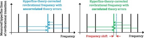
GRAPHICAL ABSTRACT
1. Introduction
Since the development of wave mechanics nearly one century ago, the three-body hydrogen molecular ion (HMI) has been a benchmark system for quantum molecular structure calculations (for a historical overview, see [Citation1]). A number of milestones in the development of the HMI molecular theory – in particular concerning methods for performing nonadiabatic calculations – were achieved by Kołos and Wolniewicz [Citation2], and later by Wolniewicz and Poll [Citation3–5]. With the advent of fully nonadiabatic three-body nonrelativistic calculations around the turn of the millennium, and the subsequent evaluation of high-order relativistic and quantum electrodynamics (QED) corrections, the state of the art has now advanced to the point where transition frequencies of rotational and vibrational transitions in the HMI electronic ground state can be computed with a theoretical uncertainty of the order of 10 parts per trillion (ppt) [Citation6,Citation7]. This level of precision is remarkable because for the first time, the uncertainty of theoretical transition frequencies is no longer limited by the uncertainty contribution from quantum molecular theory, but rather by the uncertainty introduced by the value of the proton-electron mass ratio, , published by the Committee on Data of the International Science Council (CODATA) [Citation8]. In 1976, Wing et al. had already suggested that under such conditions, it may be possible to derive an improved value of
provided that sufficiently accurate experimental transition frequencies are available [Citation9], a suggestion that was more recently extended by Karr et al. to include other physical constants as well [Citation10].
In 2020, measurements performed on the deuterated HMI, , were reported, including frequency values of a vibrational overtone [Citation11] and of a rotational transition [Citation12], with relative uncertainties of 3 ppt and 17 ppt, respectively. Both experiments made use of ion traps and sympathetic cooling and detection of
via laser-cooled beryllium ions, in combination with techniques for Doppler-free spectroscopy. For the
:
vibrational overtone (where v and N stand for the vibrational and rotational quantum numbers, respectively), Doppler-free laser excitation in the Lamb-Dicke regime was achieved using counter-propagating lasers with similar wavelengths [Citation11,Citation13]. For the
:
transition, it was the relatively long wavelength of the terahertz radiation used for rotational spectroscopy that enabled Doppler-free excitation. The results of each of the experiments were combined with theoretical calculations to derive a value of
with an unprecedented relative uncertainty of
. More recently, a measurement of the
:
rovibrational transition in
was reported, also with sufficient accuracy for a meaningful derivation of
[Citation14]. The three high-resolution measurements [Citation11,Citation12,Citation14] were later combined with other spectroscopic data from three-body systems by Germann et al. to set bounds on the validity of QED and possible manifestations of physics beyond the standard model [Citation15]. In this particular analysis, Germann et al. used values from independent determinations of
, and of the deuteron-proton mass ratio,
, to evaluate the theory [Citation16–20].
Whether it is the goal to test QED or to determine , rotational or rovibrational transition frequencies need to be measured. In practice, however, experimentally accessible transition frequencies also contain large shifts (of the order of 100 MHz) due to hyperfine structure in the lower and upper rovibrational levels. The measured frequencies therefore need to be corrected for these hyperfine shifts, in order to obtain the spin-averaged rovibrational transition frequency. In the absence of experimental data on the hyperfine structure for the transitions considered here, various approaches have been developed that all make use of theoretical ab initio predictions of the
hyperfine structure. The theoretical hyperfine structure has been computed with an uncertainty of the order of 1 kHz [Citation21,Citation22], which is comparable to the experimental uncertainty achieved in the
:
vibrational spectroscopy [Citation11]. However, rotational spectroscopy of hyperfine components of the
:
transition has been carried out with a much smaller uncertainty of 17 Hz [Citation12]. Correcting these transitions using the theoretical hyperfine shifts would reduce the accuracy by nearly two orders of magnitude, to about 1 kHz. This issue is circumvented through an approach that exploits the tracelessness of the effective spin interaction Hamiltonian that is used to compute the energies of hyperfine levels: by measuring a suitable selection of hyperfine components, and constructing a composite transition frequency by taking an appropriately weighted sum of the measured frequencies, the uncertainty of the hyperfine structure can be made to cancel out to a large extent [Citation12,Citation23]. It was pointed out by Alighanbari et al. that in this process, one has to make assumptions about (possibly) correlated uncertainties of the lower- and upper-level hyperfine energies [Citation12]. The experimental frequency value of the
:
spin-averaged transition was eventually derived for one specific correlation scenario, in which such correlations were assumed to be absent. However, the possible effect (in terms of frequency shift and frequency ucertainty) of other conceivable correlation scenarios on this result was not quantitatively discussed [Citation12].
Correlations between theory errors have been considered for atomic hydrogen and deuterium, which have traditionally played a dominant role in CODATA adjustment of the Rydberg constant, and proton and deuteron electric charge radii. For these atomic systems, the theory permits identifying state-independent and state-dependent uncertainties for the various uncalculated terms, resulting into unambiguous correlation coefficients [Citation8]. Such an approach could to some extent be employed for the HMIs as well. For rovibrational states of , however, the nature of higher-order terms can differ substantially for lower and upper vibrational states [Citation24]; see also Section 2.2 below. In addition, both recent
measurements revealed deviations between the theoretically predicted and experimentally determined hyperfine structure [Citation11,Citation12,Citation22]. Such deviations might point to a missed term in the theory, the nature of which is unknown, such that correlation coefficients cannot be reliably estimated.
Here we introduce a different approach, based on a least-squares adjustment of the spin-averaged transition frequency to an arbitrary selection of experimentally observed hyperfine components and the corresponding theoretical expressions. The above-mentioned correlations can be taken into account through the covariance matrix of the input data. The least-squares adjustment automatically takes advantage of the tracelessness of the effective spin Hamiltonian (which enters the adjustment through the theoretical expressions for the hyperfine shifts), and produces results with the same precision as the composite frequency method put forward in Refs. [Citation12,Citation23]. However, our analysis also reveals that, in general, the adjusted spin-averaged frequency may vary significantly depending on the assumed correlation coefficients. As such it lays bare a hitherto unrecognised systematic effect (which is of relevance to the both the results published by Alighanbari et al. and Patra et al.) that should be taken into consideration when determining spin-averaged transition frequencies, and derived quantities such as the value and uncertainty of from
. We also find that the
value produced by the least-squares adjustment can be helpful in establishing which correlation scenarios are consistent with the observed data, and which other correlation scenarios are less likely. To obtain a quantitative measure of the newly identified 'correlation shift' and the additional uncertainty associated with it, we carry out a Monte-Carlo simulation that takes advantage of relative weights that can be derived from the
values.
This article is organised as follows. The least-squares adjustment used to separate rovibrational and hyperfine contributions is introduced in Section 2, along with the theoretical model of the hyperfine structure. In the same chapter, the covariance between different hyperfine components is derived, and the various types of correlation involved are discussed. In Section 3, the results of the adjustment (considering various correlation scenarios) and of the Monte-Carlo runs are given for both the
:
and
:
transitions described in Refs. [Citation11,Citation12]. The impact of correlations on the spin-averaged transition frequencies and the interpretation of the Monte-Carlo results are discussed in Section 4, followed by concluding remarks in Section 5.
2. Separating hyperfine shifts from rovibrational transition frequencies
Let denote an experimentally determined frequency of a given rotational or rovibrational transition within the
electronic ground state of
. The superscripts i and j are used to label the hyperfine state of the lower and upper level, respectively. Below it will become clear that these superscripts actually represent a set of five quantum numbers that uniquely identify each state. Furthermore, we will loosely use the term 'rovibrational' to indicate vibrational as well as rotational transitions. From molecular theory it is known that
can be written as the sum of the pure rovibrational transition frequency (also known as the spin-averaged rovibrational transition frequency),
, and the hyperfine frequency shift,
. This separation is useful for various reasons. First, it can be used to determine an 'experimental' spin-averaged transition frequency,
, which may be readily compared with the theoretical prediction of the same quantity,
, in order to test the theory. Second,
is a function of
(as well as other physical constants; see Section 4). Hence,
can be determined from the comparison between theory and experiment by solving the equation
.
To determine from a single measured hyperfine component of a rovibrational transition, we can solve the equation
(1)
(1) provided that the hyperfine shift
is known. For the rovibrational states of
considered here, however, no independent experimental data exists on the hyperfine structure. Instead, we can use the theoretical hyperfine structure, which has been calculated with an uncertainty of the order of 1 kHz, or
relative to the hyperfine splitting (
GHz) [Citation21,Citation22].
In each of the recent experiments [Citation11,Citation12], a number of hyperfine components were measured. Identifying each component by the pair of quantum labels ij, we can form a set of M equations of the form
(2)
(2) The dotted equal sign indicates that the two sides of each equation are in general found to be only approximately equal, because the set of equations is overdetermined. If we again use the hyperfine shifts
from theory, then the value of
can be found by a least-squares adjustment based on Equation (Equation2
(2)
(2) ). In what follows, we will use the terminology of the CODATA least-squares adjustments [Citation25], and refer to Equation (Equation2
(2)
(2) ) as 'observational equations'.
2.1. Hyperfine structure of 
In , the hyperfine structure arises from magnetic interactions between the proton, deuteron, electron, and molecular rotation, as well as the interaction of the deuteron electric quadrupole moment with the molecular internal electric field gradient. These interactions are described (to lowest order) by the Breit-Pauli Hamiltonian, but in practice it is more convenient to capture all interactions within an effective spin Hamiltonian that is specific to a given rovibrational state v, N. The currently most elaborate version of the effective spin Hamiltonian contains nine interaction terms [Citation26]. The strength of each of the nine terms is characterised by a spin coefficient,
(
), which are obtained numerically by averaging the corresponding terms of the Breit-Pauli Hamiltonian, as well as possible high-order terms derived using the nonrelativistic quantum electrodynamics (NRQED) approach, over the rovibrational wavefunction [Citation21,Citation22,Citation26].
To find the eigenvalues of the effective spin Hamiltonian, we choose a basis set of pure spin states . The quantum numbers
, G, and F follow from the angular momentum coupling scheme
,
,
. Here,
,
, and
stand for the proton, deuteron and electron spin, respectively, with corresponding quantum numbers
,
, and
. The theoretical hyperfine level energies,
, are obtained by diagonalisation of the effective spin Hamiltonian matrix. The diagonalisation introduces some hyperfine state mixing, so that the quantum numbers
, G are only approximately good.
Obviously, the theoretical hyperfine energies are functions of the coefficients , and we express them (in frequency units) as
. Using double and single primes to indicate quantum numbers of lower and upper states, respectively, Equation (Equation2
(2)
(2) ) then takes the form
(3)
(3) To simplify notation, we will use ρ to denote the rovibrational quantum numbers v, N, and β to indicate the hyperfine quantum numbers
of a given rovibrational-hyperfine state. With this notation, the superscripts i, j in Equation (Equation1
(1)
(1) ) become
and
. The observational equations can thus be written as
(4)
(4)
2.2. Hyperfine structure: theoretical uncertainty and correlated errors
We now make the following observations regarding Equation (Equation4(4)
(4) ). First, each spin coefficient has an associated uncertainty,
. This uncertainty reflects the estimated size of the error that is made by various approximations in the theory. Although this error is not a stochastic quantity, we will follow the common practice to treat it as a normally distributed variable with zero mean and standard deviation
. Second, the observational equations are inherently correlated, since each of them depends on the same set of 18 hyperfine spin coefficients. This inherent correlation also provides the mechanism that converts the tracelessness of the effective spin Hamiltonian [Citation23] into a reduced uncertainty of the adjusted value of
. Third (and crucially), the errors of different spin coefficients may be correlated, and we can distinguish three types of correlations:
Correlated uncertainties of different spin coefficients in the same (lower or upper) rovibrational state, e.g.
Correlated uncertainties of pairs of lower-state and upper-state spin coefficients, e.g.
Correlated uncertainties of pairs of different spin coefficients, each in a different (lower or upper) state, e.g.
The uncertainties and various correlations are calculated with the help of the known functions , and included in the covariance matrix for the input data. The fractional uncertainties
are between
and
[Citation11,Citation12], which justifies using linearised expressions for
. Let
denote the transition frequency that is represented by the theoretical expression, i.e. the right-hand side of Equation (Equation4
(4)
(4) ):
Then, for any pair of transitions with theoretical frequency values
and
, the covariance matrix elements [Citation25] can be expressed as follows:
(5)
(5) The first two terms in the summation of Equation (Equation5
(5)
(5) ) contain two types of correlations. First, there are the terms with diagonal correlation coefficients (i.e. k = l) for which by definition
. These terms represent the correlation between
and
due to the shared dependence of the observational equations on the same spin coefficients, and they mediate the effect of the tracelessness of the effective spin Hamiltonian. Second, they contain terms with off-diagonal correlation coefficients (
) within the same rovibrational level (i.e. type-A correlation, for example between
and
). The third term in Equation (Equation5
(5)
(5) ) describes the covariance due to correlations
between similar spin coefficients (k = l, type B) and different (
, type C) spin coefficients in the lower- and upper-state theoretical expressions. As pointed out above, the values of the various correlation coefficients r are a priori unknown (except for the diagonal coefficients), and we will assign values
to them depending on the scenario under consideration.
We will only consider correlations for the five largest spin coefficients. These are (for the electron spin-rotation interaction),
and
(related to the aforementioned Fermi-contact terms), and
,
, which represent the tensor part of the proton-electron and deuteron-electron dipolar magnetic interactions, respectively. The spin coefficients for the proton spin-rotation (
), deuteron spin-rotation (
), proton-deuteron spin-spin tensor (
), and deuteron electric quadrupole (
) interaction have uncertainties that are negligible compared to any other uncertainty involved in the observational equations (including the experimental uncertainty). Therefore, correlation coefficients involving these spin coefficients are set to zero. Furthermore, we will assume that the uncertainties of the various experimental transition frequencies are uncorrelated. It should be noted that for the v = 0, N = 0 state, only
and
have nonzero values [Citation26]. As a consequence, for the
:
transition, type-B and type-C correlations only occur for these two spin coefficients.
We here also introduce the correlation coefficients ,
, and
. These are associated with the coefficients r in Equation (Equation5
(5)
(5) ) as follows (grouped by type A,B or C):
Type-A and type-C correlations are only considered for the large spin coefficients which describe similar interactions, i.e.
and
. This implies that we always set (for example)
. Note also that the definitions of
and
above are somewhat restrictive as they imply
for all k, and likewise for
, i.e. they assign the same value to correlation coefficients which in reality may not be necessarily equal. This restriction does not appreciably affect the results and insights obtained here, as was verified using computations with a greater flexibility in the different correlation coefficients. We nevertheless choose to work with the simplified (yet more restrictive) scenarios represented by the three coefficients
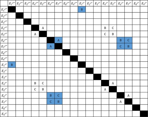
, as it makes the analysis more comprehensible. To aid the reader, a graphical overview of all nonzero correlation coefficients is provided in Figure of Appendix 1.
2.3. Least-squares adjustment
The least-squares adjustment is implemented as done for the CODATA adjustments (see Appendix E of Mohr et al. [Citation25]). Of special interest is the covariance matrix, V, of the input data, through which the various types of correlation are incorporated. Specifically, we will consider scenarios with various amounts of correlation of type A, B, and C, which are denoted by the tuple . We use the theoretical spin-averaged transition frequency,
, as starting value for the adjusted parameter
. Since the observational equations [Equation (Equation2
(2)
(2) )] are linear in
, a single adjustment suffices and no iterations are needed. The adjustment produces the adjusted value,
, and its uncertainty,
. In addition, it produces several other useful quantities, such as the normalised residuals
(6)
(6) as well as the
value [Citation25]. The associated number of degrees of freedom equals the number of observational equations (M) minus the number of adjusted constants (which equals 1 in this case, so that we have M−1 degrees of freedom).
In Appendix 2, a different approach to incorporating correlation coefficients in the least-squares adjustment is discussed. This method explicitly considers the errors of the theoretical spin coefficients, , and includes these as adjustable parameters. This approach is similar to that employed by CODATA, and it produces similar results for the adjusted values of
and
, as well as the
value.
2.4. Cases considered in this work
Here, we will consider two recent cases, namely the terahertz rotational spectroscopy of as reported by Alighanbari et al. [Citation12], and the laser vibrational spectroscopy of
by Patra et al. [Citation11]. Alighanbari et al. measured the transition frequencies of M = 6 hyperfine components of the
:
transition. We will contract the previously used superscript ij into a single superscript
to indicate the six transition frequencies
. In order to determine
, Alighanbari et al. combined the six frequencies into a composite frequency,
, given by
With the condition
, this can be written as [Citation12]
(7)
(7) Owing to the tracelessness of the effective spin Hamiltonian, the terms in the sum in Equation (Equation7
(7)
(7) ) largely cancel. Moreover, the uncertainty introduced through the sum is minimised by an appropriate choice of the coefficients
, which are determined numerically using a procedure that is conceptually similar to a least-squares minimisation. From Equation (Equation7
(7)
(7) ), the value of
is subsequently obtained [Citation12]. Alighanbari et al. also argued that from a theoretical viewpoint, strong correlations between some spin coefficients may be suspected. However, they did not quantify the effect of such possible correlations on the found value and uncertainty of
. Below, we will determine
in an alternative way, through a direct least-squares adjustment to
, thus enabling a quantitative treatment of the effect of correlations.
The other work considered here, that of Patra et al., involves measurements of M = 2 hyperfine components of the :
transition. Rather than performing an adjustment, they determined
for each value of n = 1, 2, and then computed the weighted mean of the two resulting values of
. However, contrary to expectations, they found the two values
to be in disagreement by about 7 kHz or
. Patra et al. subsequently expanded the theoretical uncertainties
by a uniform factor of
to reduce the discrepancy to
, which is commonly considered an 'acceptable' deviation. In this way, the
discrepancy became absorbed in the larger resulting uncertainty of
. Patra et al. did take into account correlations due to the shared dependence of the theoretical hyperfine shifts
on the same set of spin coefficients
, but they did not consider correlations between the spin coefficients themselves [i.e. they effectively considered a scenario (
]. In this work, we will re-analyse the results of Patra et al. using a least-squares adjustment to find
, this time also considering the effect of (different types) of correlation.
3. Results
We have analysed the two cases in the following ways. First, we have performed the adjustment for possible correlation scenarios
, with each of the coefficients
,
,
set to either 0 or 1. These scenarios include one scenario described by Alighanbari et al., who pointed out that correlation coefficients of type B are expected to be close to 1 for spin coefficients
[Citation12]. At the same time, we emphasise here that estimated theoretical errors are by definition uncertain, as are their correlation coefficients. For example, past research has shown that estimated errors sometimes do not include all the physics that plays a significant role, including unknown state-dependent error contributions that vary with v, N [Citation24]. Such errors could reduce the type-B correlation identified by Alighanbari et al. To fully appreciate the possible effect of correlations, one should therefore consider other scenarios for which
,
, and
have different independent values, potentially in a range as wide as
.
We address this issue in the second step of our analysis with the help of Monte-Carlo simulations, where each of the coefficients is selected pseudo-randomly from the interval
, after which the adjustment is performed. Repeating this 50,000 times provides insight in the distribution of adjusted values
and, through the
value of each adjustment, the relative probability of finding the value
for the corresponding coefficients
, and given the set of observed transition frequencies. This probability is obtained by inserting the found value of
in the
probability density function for
degrees of freedom, i.e. we compute the value of
with Γ the gamma function, by inserting
. The thus found probabilities will later be used as (normalised) weights, w. Note that as an alternative to the Monte-Carlo runs, we could have carried out the same calculations based on a three-dimensional grid of evenly spaced values
. However, such a grid leads to an undesired rasterization of collections of data points in two-dimensional charts, which reduces the resolution of such charts (as compared to collections of data points that are quasi-continuously distributed).
To facilitate the comparison with earlier published results, the theoretical hyperfine structure and corresponding covariances were evaluated using the spin coefficients published by Alighanbari et al. [Citation12] and Patra et al. [Citation11], and not with the updated spin coefficients that were published more recently [Citation21,Citation22].
3.1. Results : transition
Figure shows the results of the adjustment for eight scenarios involving discrete values (0 or 1) of the correlation coefficients . For the
:
transition [Figure (a,b)] a new expansion factor η was determined before each adjustment. The procedure to determine η used here differs from that deployed by Patra et al. In keeping with CODATA practice, we now uniformly expand the entire covariance matrix (expanding not only the theoretical but also the experimental uncertainty) by a factor
such that none of absolute values of the normalised residuals exceeds 2 [Citation8]. Most expansion factors η are between 1.5 and 2.7, depending on the correlation scenario, with one exception of
for the
case, which corresponds to a physically unlikely combination of correlation coefficients.
Figure 1. Adjustment of and
for various correlation scenarios [labelled by the tuples
]. The corresponding theoretical predictions
are those from Refs. [Citation11,Citation12] and are indicated by the vertical dashed lines, while the shaded area represents the corresponding theoretical uncertainty
. For completeness, a more recent value of
by Korobov and Karr [Citation7] is shown as a separate data point. (a) Results for the
:
transition, considering correlations only for
and
. The value of
as determined by Patra et al. [Citation11] is also indicated. (b) Same as (a), but for the
:
transition using the data of Alighanbari et al. [Citation12]. (c) Same as (a), but now considering
(type-B correlation only), and the pairs
and
. (d) Same as (b), but now including also type-A correlations between
.
![Figure 1. Adjustment of fex,sa0933 and fex,sa0001 for various correlation scenarios [labelled by the tuples (rA,rB,rC)]. The corresponding theoretical predictions fth,sa are those from Refs. [Citation11,Citation12] and are indicated by the vertical dashed lines, while the shaded area represents the corresponding theoretical uncertainty u(fth,sa). For completeness, a more recent value of fth,sa by Korobov and Karr [Citation7] is shown as a separate data point. (a) Results for the (v,N): (0,3)→(9,3) transition, considering correlations only for E4ρ and E5ρ. The value of fex,sa0933 as determined by Patra et al. [Citation11] is also indicated. (b) Same as (a), but for the (v,N): (0,0)→(0,1) transition using the data of Alighanbari et al. [Citation12]. (c) Same as (a), but now considering E1ρ (type-B correlation only), and the pairs E4ρ,E5ρ and E6ρ,E7ρ. (d) Same as (b), but now including also type-A correlations between E6ρ,E7ρ.](/cms/asset/894c29f0-8b6f-4996-901a-4832d1809427/tmph_a_2058637_f0001_oc.jpg)
In Figure (a), only correlations involving and
are considered. The
scenario in Figure (a) corresponds to the correlation assumptions made by Patra et al. The shift of this value relative to that of Patra et al. [Citation11] shows the (small) effect of our modified approach to determining the expansion factor η. Clearly, different correlation scenarios
may lead to additional shifts of
of about one standard uncertainty. If we in addition consider correlations between
,
and
, then the spread in values
becomes slightly smaller (if we exclude the
point); see Figure (c).
The results of the Monte-Carlo run are shown in Figure (a). For all adjustments during this run, we necessarily assumed the same expansion factor (); if we were to determine η for each adjustment individually, then the
values of different adjustments would become incomparable. Out of 50,000 realisations, 299 adjustments were discarded because they produced negative
values or complex-valued uncertainties
. The cause of these problematic cases can be traced back to the covariance matrix (for the correlation scenario in question), for example when correlations coincidentally lead to a much larger variance for one observational equation than for the other. For each of the remaining 49,701 realisations, the resulting value
is assigned a weight w as explained above. The distribution of weights is shown in Figure (a). Here its worth pointing out the difference between the weights (or probabilities) w, which can be regarded as a measure of the compatibility of the measured frequencies with the particular correlation scenario, and the probabilities that are expressed by the bin heights in the three-dimensional histogram, which do not take the compatibility between measurements and correlation scenario into account. Figure (a) also shows the distribution of frequency shifts
, which for each given combination
are computed as follows:
The minimum and maximum values of
found during the run are
kHz and 2.5 kHz, respectively, which corresponds to
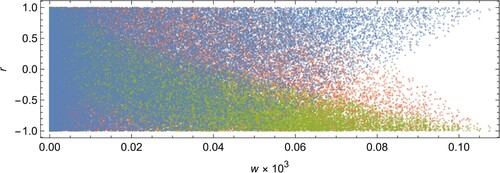
and 2.4 standard uncertainties. However, as will be discussed in Section 4, the probabilities of such strongly deviating values are small, as is their impact on the weighted mean and standard uncertainty derived from the entire set of 49,701 adjustments. The relationship between weight w and the different types of correlation
is illustrated in Figure . It can be seen that the cases with larger weight occur for positive type-A correlation, and negative type-B and type-C correlation. This forms an indication that the combination of the measured transition frequencies and the theoretical model favours such correlation scenarios.
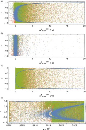
Figure 2. Results of Monte-Carlo runs. (a) :
transition, 49,701 realisations. (b)
:
transition, 49,550 realisations. (c) Zoomed-in portion of the histogram shown in (b).
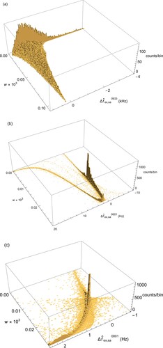
Figure 3. Weight (or probability) w versus r for the Monte-Carlo run shown in Figure (a). Although not visible from the graph, the different coloured dots occur in vertically aligned groups of three, each group corresponding to a single adjustment with correlation coefficients (blue),
(green), and
(red) (colour online only).
3.2. Results : transition
Effects of correlation are also visible in the adjustments pertaining to the :
transitions; see Figure (b,d). If we consider correlation coefficients with discrete values (0 or 1), then, depending on the correlation scenario, we find shifts by more than three standard uncertainties relative to the uncorrelated case
. The value and uncertainty of
found for the latter scenario corresponds closely to the value of
reported by Alighanbari et al. Figure (b,d). This is not unexpected because these authors also assumed uncorrelated spin coefficients in their analysis.
The spread of the adjusted frequencies in Figure appears to be considerably larger for the :
transition than for the
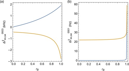
:
transition. However, closer inspection of the dependence of the shift on the coefficients r reveals that the shift may drop rapidly already for values only slightly below r = 1. This behaviour is illustrated in Figure (b) for the scenario
and the
:
transition. For values
approaching 1, the sudden rise in frequency is accompanied by
values that imply a drop in probability by orders of magnitude (not shown). For the
scenario concerning the
:
transition, the frequency dependence on
is shown in Figure (a). In this case, the frequency dependence close to
is considerably less steep than for the
:
case.
Figure 4. Dependence of the adjusted frequency on the correlation coefficient . (a)
versus
for the scenario
, and considering correlations between
and
(upper curve), and between
,
,
,
, and
(lower curve). For the upper and lower curves, the limiting cases
and
are also shown in Figure (a) and Figure (c), respectively. A uniform expansion factor
was applied. (b)
versus
for the scenario
, and considering correlations between
and
(lower curve), and between
,
,
, and
(upper curve). In this case, for the lower and upper curves, the limiting cases
and
are also shown in Figure (b) and Figure (d), respectively.
The results of the Monte-Carlo run are shown in Figure (b) and (c). As before, we define
Out of 50,000 realisations, 450 adjustments were discarded because they produced negative
values or complex-valued uncertainties
. The minimum and maximum values of
found during the run are
Hz and 320 Hz, respectively, corresponding to
and 18 standard uncertainties. However, as will be discussed in Section 4, the probabilities of such strongly deviating values are small, as is their impact on the weighted mean and standard uncertainty derived from the set of 49,550 adjustments.
A salient feature of the histogram in Figure (b) is the -distribution-like 'curve' visible in the
-plane, along which most results are found. As can be seen in Figure (a), the realisations in this part of the histogram correspond to adjustments with values of
spread around zero for values
, but with
-values becoming more concentrated and increasing smoothly to asymptotic values of
if the 'curve' is followed towards ever larger values of
. By contrast, no such smooth behaviour is seen in the values of
, which appear scattered over the range
independent of the value of
.
Figure 5. Shift of versus values of
(blue),
(green), and
(red), obtained from Monte-Carlo runs (colour online only). Although not visible from the graphs, the different coloured dots occur in vertically aligned groups of three, each group corresponding to a single adjustment with correlation coefficients
. (a) Results of a ∼50,000-point Monte-Carlo run involving
,
,
, and
. (b) Same as in (a), but now involving only
and
. (c) Same as (a), but now involving only
and
. (d) Weight (or probability) w versus r for the run involving
,
,
, and
. This run was also used to produce Figure (b).
To investigate which spin coefficients are responsible for the observed relationship between and
, the Monte-Carlo run was repeated once considering only correlations involving
and
, and once involving only
and
. The results in the
-plane are presented in Figure (b,c), respectively As is visible in Figure (c), the latter pair of coefficients is responsible for the behaviour seen in Figure (b), with their type-A correlation coefficient displaying a nearly functional dependence on
. Plotting the outcomes of the full Monte-Carlo run (i.e. involving
,
,
, and
) in the
-plane reveals that the weights peak around
and
[Figure (d)].
4. Discussion
The results in Section 3 show that if one uses a theoretical hyperfine structure model to derive the spin-averaged transition frequency from a set of measured hyperfine components of a rovibrational transition, assumptions regarding correlated errors in the theoretical spin coefficients influence the result (in our case the adjusted value of ). As correlation coefficients between various theory errors cannot be exactly known, some liberty (or rather uncertainty) exists in the choice of correlation coefficients. The consequence of this liberty is twofold: the value of
could be significantly shifted away from the value that is obtained when assuming zero correlation (as was done in Refs. [Citation11,Citation12]), and the concomitant spread of values
introduces additional uncertainty to its final value. For example, computing the mean and standard deviation of all values
in the 49,701-point Monte-Carlo run yields a shift of
kHz and a standard deviation of 0.58 kHz. While both the shift and the standard deviation are still smaller than
kHz, the effect cannot be ignored, in particular in view of some of the very large observed shifts
. Similar considerations apply to the
:
transition also studied here: taking the mean and standard deviation of all values
in the 49,550-point Monte-Carlo run yields a shift of
Hz and a standard deviation of 3.6 Hz. Again, both the shift and the standard deviation are smaller than
Hz, but also for this case the effect cannot be ignored in view of some of the very large shifts
. Our analysis furthermore shows that one should be particularly careful with scenarios where correlation coefficients r = 1 are assumed, as evidenced by the very steep frequency shifts shown in Figure (b).
4.1. Interpretation and treatment of correlation-induced shifts
We may interpret this effect in the context of observational equations, which generally contain a measured quantity in the left-hand side of the equation, and a corresponding theoretical expression in the right-hand side of the equation. Usually, all parameters of the theoretical model are included in the theoretical expression, and their values are either adjusted, or estimated using external means. In the latter case, the uncertainties of the estimated parameters (and their covariances with other parameters) are included in the covariance matrix of the input data. However, in cases where correlation coefficients are possibly nonzero but a priori unknown, the correlation coefficients themselves become parameters of the theoretical model too.
This line of reasoning implies that correlation coefficients, like all other parameters, should meet two requirements: first, they need to be assigned a value (either by some external means, or by making them adjustable parameters); second, they need be assigned an uncertainty. However, assigning a value to correlation coefficients between estimated theory errors that are intrinsically uncertain (and that may not include all relevant physics) can be considered a 'best guess' at best. The second requirement, assigning an uncertainty range to r values, might be achievable, but would most likely necessitate subjective measures such as Bayesian 'degree of belief' likelihood functions. The other option, adjusting the values of correlation coefficients themselves might be challenging too, as it may not always be possible to find a single-valued functional correspondence between r and the adjusted parameter, and because the dependence on r may exhibit strong nonlinear behaviour. This may preclude linearisation of the theoretical expression and – ultimately – the (linear) least-squares adjustment itself. On the other hand, if correlation coefficients can be adjusted, the adjustment would automatically produce their uncertainties as well.
Here we propose a pragmatic alternative approach to deal with the issues outlined above. The Monte-Carlo runs developed here provide a means to determine the spread in a way that makes no assumptions regarding the values of whatsoever. As shown above, we were able to quantify the effect of unknown correlation coefficients by computing the mean and standard deviation of all ∼50,000 values of
. In addition, we can take advantage of the capability of any least-squares adjustment to provide a (relative) measure – the
value – of the compatibility between the measurements and the theoretical model (which now also encompasses the correlation coefficients), in order to get an improved estimate of
and its uncertainty. To this end, we use the weights w to calculate means and uncertainties of the weighted results of the Monte-Carlo runs. For example, for the
:
transition, we earlier found an unweighted mean (standard deviations within parentheses) of
kHz relative to
, whereas consideration of the weights leads to a compatible but more precise value of
kHz. This should be compared with the uncertainty
kHz for the uncorrelated
scenario (with expansion factor
). Also for the
:
transition, the weighting reduces the standard deviation significantly, improving the unweighted mean and uncertainty of all values
,
Hz, to the weighted result
Hz. The standard deviation of the weighted result is negligibly small compared to
, which equals 17 Hz. The results are summarised in Table for both the
:
and
:
transitions.
Table 1. Correlation-induced shift and standard uncertainty, as obtained from unweighted and weighted results of the Monte-Carlo runs, to the :
and
:
spin-averaged transition frequencies.
Furthermore, the three-dimensional histogram in Figure (b) indicates that most values are located along the
-like curve with frequency offsets between 0 Hz and 2.5 Hz. Two peaks are visible: a primary one around
, and a secondary one around
. From Figure (a) it can be seen that for the secondary peak (i.e. for
Hz),
attains values close to 0.76 or
. These values are the ones with the largest weight w in Figure (d), a behaviour that is due to the coefficients
and
. We therefore conclude that the transition frequencies measured by Alighanbari et al. are compatible with a scenario where the coefficients
and
are rather strongly correlated. Given the very similar theoretical models that are used to compute these physically related coefficients, one would indeed expect a strong correlation between their errors.
Yet, Figure (b) and Figure (a,d) show that the measured transition frequencies are also compatible with Hz for relatively small values of
, and for a wide range of values
. For these scenarios, which constitute the primary peak in Figure (b), the physical interpretation is less obvious. The occurrence of this peak is made possible by the fact that the Monte-Carlo run does not make a priori assumptions regarding the values of
, even if many combinations
might be less likely from a physical point of view. The
Hz distance between the primary and the secondary peak is therefore indicative of the uncertainty introduced through the unknown correlation coefficients.
It may furthermore be possible to develop a refined approach which includes theoretical input on the possible values of correlation coefficients. For example, anticorrelations appear very unlikely, as it has never been observed that a given NRQED correction term changes sign between two different rovibrational states (at least within the range of investigated rovibrational states studied so far). Such auxiliary information may in the future be used to truncate the range of possible values of the correlation coefficients.
4.2. Adjustment of fundamental physical constants
The correlation-induced shift and uncertainty have an effect on the value of that can be derived from the
:
and
:
transition frequencies. We calculate their impact using sensitivity coefficients computed by Karr et al. [Citation10]. To find the fractional effect (in ppt) on the value of
, we multiply the entries for the
:
transition in Table with
kHz
, and those for the
:
with
Hz
. The results are shown in Table , and we find that the correlation-induced shift and uncertainty affect the value of
at the few-ppt level. This is still one order of magnitude smaller than the
-ppt uncertainties that were reported by Patra et al. and Alighanbari et al. [Citation11,Citation12], which are dominated by the uncertainty of the theoretical values of the spin-averaged transition frequencies,
and
, respectively.
Table 2. Correlation-induced shift and standard uncertainty (in ppt), to the value of , as obtained from unweighted and weighted results of the Monte-Carlo runs.
We intentionally do not provide absolute values of here: since the publication of the three recent measurements in
[Citation11,Citation12,Citation14], no less than nine different values of
derived from these measurements have been reported. These were computed using various methods and using different choices of fundamental constants used in the
theory, and the values also depend somewhat on the state of the art of the theory at the time of publication [Citation7,Citation11,Citation12,Citation14]. Instead of extending the list of
determinations from
here by four new values, each with its own specific interpretation, we refer the reader to the overview of
-derived values of
by Korobov and Karr, who based their analysis on the most recent theory [Citation7]. It is conceivable that these values will eventually be superseded by the anticipated CODATA-2022 adjustment, which would produce a single and thoroughly justified value of
, which would be based on all relevant measurements and theory (including not only
and Penning-trap measurements, but also measurements and theory of atomic hydrogen and hydrogen-like systems for the Rydberg constant and nuclear charge radii, and measurements relevant to the fine-structure constant).
Inclusion of data in a global adjustment of fundamental physical constants such as the CODATA adjustment could proceed in the following way, by augmenting the global set of observational equations used for the adjustment with the following set of equations:
(8)
(8) To arrive at Equation (Equation8
(8)
(8) ), we replaced
in Equation (Equation4
(4)
(4) ) with the known function
[Citation10]. Here,
stands for the Rydberg constant, α for the fine-structure constant, and
and
for the proton and deuteron electric charge radii, respectively. Equation (Equation8
(8)
(8) ) would include the two
:
hyperfine components as well as the six
:
hyperfine components, and may furthermore include the two hyperfine components of the
:
transition measured by Kortunov et al. [Citation14]. The arguments of the functions
are parameters that are globally adjusted (i.e. they are adjusted to many other observational equations besides those from
, derived from measurements of other physical systems). Uncertainties and correlations can be taken into account through a covariance matrix as before, and the impact of the various correlation coefficients could be quantitatively assessed using the approach presented in this work. Alternatively, theory errors and their mutual correlations can be included by introducing additional adjustable parameters that explicitly represent the error terms [Citation8,Citation25]; see also Appendix 2.
5. Conclusion
In conclusion, we have shown that if hyperfine shifts are to be removed from measured rovibrational transtion frequencies by using theoretically calculated hyperfine structure, one needs to consider the effect of (potentially) correlated parameters in the theoretical model. To our knowledge, this constitutes a hitherto unrecognised systematic effect in molecular spectroscopy, which we here analysed using a least-squares approach that can readily take such correlations into account. We analysed the impact of this systematic effect on two recently published results obtained from high-precision spectroscopy of HD and calculated hyperfine shifts derived from an effective spin Hamiltonian. We showed that certain correlation scenarios may lead to strongly deviating values of spin-averaged rovibrational transition frequencies. To quantify the effect in terms of the corresponding frequency shift and uncertainty, we presented a Monte-Carlo approach that enables statistical averaging over many possible correlation scenarios. With the help of weights, derived from
values from the least-squared adjustment, a robust estimate of the size and uncertainty of this new systematic shift was obtained, resulting in values much smaller than the uncertainty reported earlier for the spin-averaged transition frequencies [Citation11,Citation12]. This work may be of interest to future spectroscopic studies which make use of theoretical calculations to remove hyperfine shifts, as well as potential future applications of the spectroscopic data analysed here, such as the adjustment of fundamental physical constants.
Acknowledgments
The author wishes to thank Jean-Philippe Karr for fruitful discussions and comments on the manuscript.
Disclosure statement
The author declares no conflicts of interest.
References
- A. Carrington, I.R. McNab and C.A. Montgomerie, J. Phys. B: At. Mol. Opt. Phys. 22 (22), 3551–3586 (1989). doi:10.1088/0953-4075/22/22/006
- W. Kołos and L. Wolniewicz, Rev. Mod. Phys. 35, 473–483 (1963). doi:10.1103/RevModPhys.35.473
- L. Wolniewicz and J.D. Poll, J. Mol. Spectrosc. 72 (2), 264–274 (1978). doi:10.1016/0022-2852(78)90126-1
- L. Wolniewicz and J.D. Poll, J. Chem. Phys. 73 (12), 6225–6231 (1980). doi:10.1063/1.440117
- L. Wolniewicz and J. Poll, Mol. Phys. 59 (5), 953–964 (1986). doi:10.1080/00268978600102501
- V.I. Korobov, L. Hilico and J.-Ph. Karr, Phys. Rev. Lett. 118, 233001 (2017). doi:10.1103/PhysRevLett.118.233001
- V.I. Korobov and J.-Ph. Karr, Phys. Rev. A. 104, 032806 (2021). doi:10.1103/PhysRevA.104.032806
- E. Tiesinga, P.J. Mohr, D.B. Newell and B.N. Taylor, Rev. Mod. Phys. 93, 025010 (2021). doi:10.1103/RevModPhys.93.025010
- W.H. Wing, G.A. Ruff, W.E. Lamb and J.J. Spezeski, Phys. Rev. Lett. 36, 1488–1491 (1976). doi:10.1103/PhysRevLett.36.1488
- J.-Ph. Karr, L. Hilico, J.C.J. Koelemeij and V.I. Korobov, Phys. Rev. A. 94, 050501 (2016). doi:10.1103/PhysRevA.94.050501
- S. Patra, M. Germann, J.-Ph. Karr, M. Haidar, L. Hilico, V.I. Korobov, F.M.J. Cozijn, K.S.E. Eikema, W. Ubachs and J.C.J. Koelemeij, Science. 369 (6508), 1238–1241 (2020). doi:10.1126/science.aba0453
- S. Alighanbari, G.S. Giri, F.L. Constantin, V.I. Korobov and S. Schiller, Nature. 581, 152–158 (2020). doi:10.1038/s41586-020-2261-5
- V.Q. Tran, J.-Ph. Karr, A. Douillet, J.C.J. Koelemeij and L. Hilico, Phys. Rev. A. 88 (3), 033421 (2013). doi:10.1103/PhysRevA.88.033421
- I.V. Kortunov, S. Alighanbari, M.G. Hansen, G.S. Giri, V.I. Korobov and S. Schiller, Nat. Phys. 17, 569–573 (2021). doi:10.1038/s41567-020-01150-7
- M. Germann, S. Patra, J.P. Karr, L. Hilico, V.I. Korobov, E.J. Salumbides, K.S.E. Eikema, W. Ubachs and J.C.J. Koelemeij, Phys. Rev. Research. 3, L022028 (2021). doi:10.1103/PhysRevResearch.3.L022028
- S. Sturm, F. Köhler, J. Zatorski, A. Wagner, Z. Harman, G. Werth, W. Quint, C.H. Keitel and K. Blaum, Nature. 506, 467–470 (2014). doi:10.1038/nature13026
- F. Heiße, F. Köhler-Langes, S. Rau, J. Hou, S. Junck, A. Kracke, A. Mooser, W. Quint, S. Ulmer, G. Werth, K. Blaum and S. Sturm, Phys. Rev. Lett. 119 (3), 033001 (2017). doi:10.1103/PhysRevLett.119.033001
- F. Heiße, S. Rau, F. Köhler-Langes, W. Quint, G. Werth, S. Sturm and K. Blaum, Phys. Rev. A. 100, 003400 (2019). doi:10.1103/PhysRevA.100.022518
- D.J. Fink and E.G. Myers, Phys. Rev. Lett. 124, 013001 (2020). doi:10.1103/PhysRevLett.124.013001
- S. Rau, F. Heiße, S. Köhler-Langes, F. Sasidharan, R. Haas, D. Renisch, C.E. Düllmann, W. Quint, S. Sturm and K. Blaum, Nature. 585, 43–47 (2020). doi:10.1038/s41586-020-2628-7
- V.I. Korobov, J.-Ph. Karr, M. Haidar and Z.X. Zhong, Phys. Rev. A. 102, 022804 (2020). doi:10.1103/PhysRevA.102.022804
- J.-Ph. Karr, M. Haidar, L. Hilico, Z.X. Zhong and V.I. Korobov, Phys. Rev. A. 102, 052827 (2020). doi:10.1103/PhysRevA.102.052827
- S. Schiller and V.I. Korobov, Phys. Rev. A. 98, 022511 (2018). doi:10.1103/PhysRevA.98.022511
- V.I. Korobov, J.C.J. Koelemeij, L. Hilico and J.-Ph. Karr, Phys. Rev. Lett. 116 (5), 053003 (2016). doi:10.1103/PhysRevLett.116.053003
- P.J. Mohr and B.N. Taylor, Rev. Mod. Phys. 72, 351–495 (2000). doi:10.1103/RevModPhys.72.351
- D. Bakalov, V.I. Korobov and S. Schiller, Phys. Rev. Lett. 97 (24), 243001 (2006). doi:10.1103/PhysRevLett.97.243001
Appendices
Appendix 1: Overview of nonzero correlation coefficients
Figure provides a graphical overview of the correlation coefficients that are assigned nonzero values, and how they relate to the different types of correlation identified in this work.
Figure A1. Graphical overview of correlation coefficients. Empty cells correspond to correlation coefficients which are always set to zero, either because the corresponding covariances are negligibly small on an absolute frequency scale, or because the spin coefficients involved are unlikely to be uncorrelated as they represent physically distinct interactions. Nonzero correlations of type A, B and C are indicated. Cells with a shaded background correspond to correlations that are nonzero only in the :
analysis.
Appendix 2: Including theory errors as adjustable parameters
It is possible to formulate the least-squares problem in a slightly different form, which is due to CODATA. In this case, we define 18 additional adjustable parameters, , which represent the errors of the 18 spin coefficients
for the lower and upper states. We propagate and add these errors to the observational equations [Equation (Equation4
(4)
(4) )] as follows:
(A1)
(A1) Furthermore, we add 18 observational equations of the form
. Note that for the
:
transition, the number of spin coefficients is only 11, and the number of parameters
(as well as the number of corresponding observational equations) is reduced accordingly. The covariance matrix of input data is now composed of the individual terms from the summations in Equation (Equation5
(5)
(5) ). Performing this alternative least-squares adjustment results into values
,
, and
that are identical to the results obtained using the approach of Section 2. In addition, values of the errors
are produced. This alternative method, however, produces singular covariance matrices V for some scenarios where
,
, and/or
equal 1. These matrices cannot be inverted, and therefore in such cases the adjustment cannot be carried out. For this reason, the least-squares approach of Section 2 was preferred in this work.