Spin-density calculation via the graphical unitary group approach

Abstract

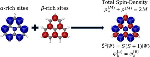
In this work we discuss the calculation of the spin-density matrix from fundamental spin principles as implemented in the COLUMBUS Program System employing the graphical unitary group approach (GUGA). First, a general equation for the spin-density matrix is derived in terms of the one-and two-particle reduced density matrices, quantities that are spin-independent and readily available within the GUGA formalism. Next, the evaluation of this equation using the Shavitt loop values is discussed. Finally, the spatially resolved counterpart of the spin-density matrix, the spin distribution, is calculated for the phenalenyl radical and structures produced by heteroatoms with mono- and di-substitutions. The physical meaning of the spin-density along with its computational description using various methods is discussed putting special emphasis on negative contributions to the spin-density and their quantification via a spin-promotion index.

GRAPHICAL ABSTRACT

Keywords:

• Graphical unitary group approach
• spin-density
• phenalenyl
• spin-promotion index

1. Introduction

Modern multiconfigurational electronic structure methods applied to molecules rely typically on configuration state functions (CSFs) as a basis for the expansion of the many-body wave function that describes the spatial and spin distributions of the system. The graphical unitary group approach (GUGA) [1–5] can be employed to construct a CSF expansion space that makes no reference to its determinantal representation. In this formalism, each CSF may be represented as a walk from the tail to the head of a Shavitt graph, or as a sequence of nodes within the graph, or as a step vector containing the occupation and spin coupling of each spatial orbital.

In the absence of external fields, the nonrelativistic molecular Hamiltonian operator commutes with the spin operators ${\hat{S}}^2$ and ${\hat{S}}_z$, and consequently the CSF expansion can be limited to include only terms that contribute to the overall target spin, defined by the quantum number S. Moreover, given the quantum number M related to the spin projection on the z-axis, the energy values for the 2S + 1 members of the multiplet are degenerate.

GUGA takes advantage of these above mentioned properties, since it is a spin-free formalism that completely suppresses the quantum number M from the computational procedure. However, this spin-free approach introduces difficulties in the calculation of spin-dependent properties such as the spin-density. A first approach to obtain these spin-dependent properties would be to transform the wave function from the CSF basis to the Slater determinant basis that depends on M, and then to compute the property expectation value in that representation. This approach becomes inefficient for large expansions, since the determinantal basis is larger and increases faster than the CSF basis with molecular size. The best approach is to compute the spin-dependent properties directly within the GUGA formalism, making the effort to compute spin-dependent properties similar to that for spin-independent properties.

The spatial spin-density distribution is widely used to represent the active or unpaired electrons of an electronic state pictorially [6–9]. More specifically, the spin-density matrix and the resultant spatial spin-density distribution are useful for spectroscopic properties of electron paramagnetic resonance, determining the nuclear hyperfine coupling constants [10–13]. Moreover, shifts in paramagnetic nuclear resonance depend on the spin density at a nucleus [12–16].

Spin-density distributions obtained from density functional theory calculations can be sensitive to the choice of functional [7, 17–19]. In this scenario, an ab initio approach to obtain reliable spin-densities is essential to achieve unambiguous results [8]. Furthermore, accurate ab initio spin-density distributions could be used for developing density functional theory (DFT), especially in the spin-DFT formalism proposed by von Barth and Hedin [20]. In this framework, the spin-density is employed as a fundamental property, and highly accurate results could be employed as benchmarks to construct reliable exchange-correlation functionals that approximate the exact molecular electronic structure.

The main goal of this article is to describe how to obtain the spin-density matrix within the GUGA formalism and to present results acquired from the new implementation in the Columbus Program System [5, 21–23]. The current implementation focuses on multiconfiguration self-consistent field (MCSCF) calculations, but it may be directly extended also to multireference configuration interaction (MRCI) and multireference average quadratic coupled cluster (MR-AQCC) calculations.

An interesting molecule to explore the recently added spin-density function in Columbus is the phenalenyl (PLY) radical, C₁₃H₉. PLY is an open-shell non-Kékule molecule composed of three fused benzene rings with a triangular topology containing 13 π-electrons. This molecule is studied widely due to its fascinating electronic structure properties [24, 25], its role in soot formation [26, 27], as well as potential applications in energy storage [28] and organic electronics [29, 30]. Structural changes to PLY by incorporating heteroatoms into the structure drastically affects the electronic properties due to the change of the number of π-electrons and to the delocalisation of the unpaired electron [31]. Furthermore, modified phenalenyl provides the interesting possibility of inverted singlet-triplet gaps (i.e. $S_1$ lying below $T_1$) [32].

2. Methods

2.1. Spin-density matrices

In this section, the spin algebra will be reviewed and the equation to obtain the spin-density matrix from the one-particle and two-particle reduced density matrices (RDM) will be derived. For more details about this subject, the reader is referred to Ref. [33].

A wave function $|\psi ;S,M〉$ is an eigenfunction of the operator ${\hat{S}}^2$ with quantum number $S\ge 0$, (1) ${\hat{S}}^2|\psi ;S,M〉=S(S+1)|\psi ;S,M〉,$(1) and of the operator ${\hat{S}}_z$ that determines the projection on the z-axis with quantum number $M=-S,-S+1,\dots ,S-1,S$ as (2) ${\hat{S}}_z|\psi ;S,M〉=M|\psi ;S,M〉.$(2) Atomic units, in which $\hslash =1$, are used herein. The quantum numbers S and M assume integer values for even numbers of electrons N and half-integer values for odd N.

It is usual to define the raising and lowering operators (${\hat{S}}_{+}={\hat{S}}_x+i{\hat{S}}_y$ and ${\hat{S}}_{-}={\hat{S}}_x-i{\hat{S}}_y$) to further develop the projections of the spin along the axes. A same-orbital-for-different-spins (SODS) spin-orbital basis of dimension $2n$ is defined as $\left\{{\phi }_k\right(\mathbf{r}):k=1\dots n\}\otimes \{\alpha ,\text{β}\}$ where ${\phi }_k\left(\mathbf{r}\right)$ is an orthonormal molecular orbital (MO), and α and β are the two single-electron spin functions $|1/2,\pm 1/2〉$. A member of this set is denoted ${\phi }_{k\sigma }\equiv {\phi }_k\left(\mathbf{r}\right)\sigma$ with $\sigma \in \{\alpha ,\text{β}\}$. Employing the second quantisation, creation and annihilation operators are denoted in this spin-orbital basis as ${\hat{a}}_{k\sigma }^{†}$ and ${\hat{a}}_{k\sigma }$. These operators satisfy the anticommutation relations (3) $\begin{array}{rl}{[{\hat{a}}_{p\sigma }^{†},{\hat{a}}_{q\mu }^{†}]}_{+}& ={[{\hat{a}}_{p\sigma },{\hat{a}}_{q\mu }]}_{+}=0,\\ {[{\hat{a}}_{p\sigma }^{†},{\hat{a}}_{q\mu }]}_{+}& ={\delta }_{pq}{\delta }_{\sigma \mu },\end{array}$(3) and particle-number conserving single-excitation operators of the form ${\hat{a}}_{p\sigma }^{†}{\hat{a}}_{q{\sigma }^{\mathrm{\prime }}}$ satisfy the commutation relation (4) $[{\hat{a}}_{p\sigma }^{†}{\hat{a}}_{q{\sigma }^{\mathrm{\prime }}},{\hat{a}}_{r\mu }^{†}{\hat{a}}_{s{\mu }^{\mathrm{\prime }}}]={\hat{a}}_{p\sigma }^{†}{\hat{a}}_{s{\mu }^{\mathrm{\prime }}}{\delta }_{qr}{\delta }_{{\sigma }^{\mathrm{\prime }}\mu }-{\hat{a}}_{r\mu }^{†}{\hat{a}}_{q{\sigma }^{\mathrm{\prime }}}{\delta }_{ps}{\delta }_{\sigma {\mu }^{\mathrm{\prime }}}.$(4) It is convenient to collect the four SODS single-excitation operators ${\hat{a}}_{p\alpha }^{†}{\hat{a}}_{q\alpha }$, ${\hat{a}}_{p\alpha }^{†}{\hat{a}}_{q\text{β}}$, ${\hat{a}}_{p\text{β}}^{†}{\hat{a}}_{q\alpha }$, and ${\hat{a}}_{p\text{β}}^{†}{\hat{a}}_{q\text{β}}$ into spin-tensor form [34, 35]: (5) $\begin{array}{rl}{\hat{T}}_{pq}^{0,0}& =\frac{1}{\sqrt{2}}({\hat{a}}_{p\alpha }^{†}{\hat{a}}_{q\alpha }+{\hat{a}}_{p\text{β}}^{†}{\hat{a}}_{q\text{β}})=\frac{1}{\sqrt{2}}{\hat{E}}_{pq},\\ {\hat{T}}_{pq}^{1,1}& =-{\hat{a}}_{p\alpha }^{†}{\hat{a}}_{q\text{β}},\\ {\hat{T}}_{pq}^{1,0}& =\frac{1}{\sqrt{2}}({\hat{a}}_{p\alpha }^{†}{\hat{a}}_{q\alpha }-{\hat{a}}_{p\text{β}}^{†}{\hat{a}}_{q\text{β}}),\\ {\hat{T}}_{pq}^{1,-1}& ={\hat{a}}_{p\text{β}}^{†}{\hat{a}}_{q\alpha },\end{array}$(5) with one singlet operator and the three components of a triplet operator. The ${\hat{E}}_{pq}$ singlet operator is a generator of the unitary group and is discussed below. With these factors and phases, the spin-tensors satisfy the standard relations (6) $\begin{array}{rl}({\hat{T}}_{pq}^{S,M}{)}^{†}& =(-1{)}^M{\hat{T}}_{qp}^{S,-M},\\ [{\hat{S}}_{\pm },{\hat{T}}_{pq}^{S,M}]& =\sqrt{S(S+1)-M(M\pm 1)}{\hat{T}}_{pq}^{S,M\pm 1},\\ [{\hat{S}}_z,{\hat{T}}_{pq}^{S,M}]& =M{\hat{T}}_{pq}^{S,M}.\end{array}$(6) The ‘±’ convention in this equation and hereafter is that either the sequence of top signs or the sequence of bottom signs may be taken. This spin-tensor notation is useful because it allows the normal spin-coupling relations to be used for operator-operator, wavefunction-wavefunction, and operator-wavefunction products. In particular, matrix elements of the form $〈{\psi }^{\mathrm{\prime }};S_3,M_3|{\hat{T}}_{pq}^{S_2,M_2}|\psi ;S_1,M_1〉$ can be nonzero only when $M_3=M_1+M_2$ and when the three spin values $S_1$, $S_2$, and $S_3$ satisfy the triangle inequality, e.g. $|S_1-S_2|\le S_3\le S_1+S_2$. In the spin-orbital basis, the spin operators can be written as (7) $\begin{array}{rl}{\hat{S}}_z& =\frac{1}{2}\sum _k({\hat{a}}_{k\alpha }^{†}{\hat{a}}_{k\alpha }-{\hat{a}}_{k\text{β}}^{†}{\hat{a}}_{k\text{β}})\\ & =\frac{1}{2}({\hat{N}}_{\alpha }-{\hat{N}}_{\text{β}})=\frac{1}{\sqrt{2}}\sum _k{\hat{T}}_{kk}^{1,0},\\ {\hat{S}}_{+}& ={\hat{S}}_{-}^{†}=\sum _k{\hat{a}}_{k\alpha }^{†}{\hat{a}}_{k\text{β}}=-\sum _k{\hat{T}}_{kk}^{1,1},\\ {\hat{S}}_{-}& ={\hat{S}}_{+}^{†}=\sum _k{\hat{a}}_{k\text{β}}^{†}{\hat{a}}_{k\alpha }=\sum _k{\hat{T}}_{kk}^{1,-1}.\end{array}$(7) ${\hat{N}}_{\sigma }$ is the number operator for σ type electrons, and it commutes with any operator that conserves the number of σ electrons. The total number operator $\hat{N}={\hat{N}}_{\alpha }+{\hat{N}}_{\text{β}}$ commutes with any operator that conserves the total number of electrons.

The application of these spin operators to a wave function results in (8) $\begin{array}{rl}{\hat{S}}_{\pm }|\psi ;S,M〉& =\sqrt{S(S+1)-M(M\pm 1)}|\psi ;S,M\pm 1〉,\\ & =\sqrt{(S\pm M+1)(S\mp M)}|\psi ;S,M\pm 1〉.\end{array}$(8) The ${\hat{S}}^2$ operator may be written as (9) $\begin{array}{rl}{\hat{S}}^2& ={\hat{S}}_x^2+{\hat{S}}_y^2+{\hat{S}}_z^2,\\ & =\frac{1}{2}({\hat{S}}_{+}{\hat{S}}_{-}+{\hat{S}}_{-}{\hat{S}}_{+})+{\hat{S}}_z^2,\\ & ={\hat{S}}_{\mp }{\hat{S}}_{\pm }+{\hat{S}}_z({\hat{S}}_z\pm 1).\end{array}$(9) The commutation relations, (10) $\begin{array}{rl}[{\hat{S}}^2,{\hat{S}}_z]& =[{\hat{S}}^2,{\hat{S}}_{\pm }]=0,\\ [{\hat{S}}_z,{\hat{S}}_{\pm }]& =\pm {\hat{S}}_{\pm },\\ [{\hat{S}}_{+},{\hat{S}}_{-}]& =2{\hat{S}}_z,\end{array}$(10) follow from Equations (6(6) $\begin{array}{rl}({\hat{T}}_{pq}^{S,M}{)}^{†}& =(-1{)}^M{\hat{T}}_{qp}^{S,-M},\\ [{\hat{S}}_{\pm },{\hat{T}}_{pq}^{S,M}]& =\sqrt{S(S+1)-M(M\pm 1)}{\hat{T}}_{pq}^{S,M\pm 1},\\ [{\hat{S}}_z,{\hat{T}}_{pq}^{S,M}]& =M{\hat{T}}_{pq}^{S,M}.\end{array}$(6) ) and (7(7) $\begin{array}{rl}{\hat{S}}_z& =\frac{1}{2}\sum _k({\hat{a}}_{k\alpha }^{†}{\hat{a}}_{k\alpha }-{\hat{a}}_{k\text{β}}^{†}{\hat{a}}_{k\text{β}})\\ & =\frac{1}{2}({\hat{N}}_{\alpha }-{\hat{N}}_{\text{β}})=\frac{1}{\sqrt{2}}\sum _k{\hat{T}}_{kk}^{1,0},\\ {\hat{S}}_{+}& ={\hat{S}}_{-}^{†}=\sum _k{\hat{a}}_{k\alpha }^{†}{\hat{a}}_{k\text{β}}=-\sum _k{\hat{T}}_{kk}^{1,1},\\ {\hat{S}}_{-}& ={\hat{S}}_{+}^{†}=\sum _k{\hat{a}}_{k\text{β}}^{†}{\hat{a}}_{k\alpha }=\sum _k{\hat{T}}_{kk}^{1,-1}.\end{array}$(7) ).

It is useful to link the spin operators to the generators of the unitary group [2, 4]. This generator may be defined with no reference to spin [36], but here it is convenient to use the formulation in Equation (5(5) $\begin{array}{rl}{\hat{T}}_{pq}^{0,0}& =\frac{1}{\sqrt{2}}({\hat{a}}_{p\alpha }^{†}{\hat{a}}_{q\alpha }+{\hat{a}}_{p\text{β}}^{†}{\hat{a}}_{q\text{β}})=\frac{1}{\sqrt{2}}{\hat{E}}_{pq},\\ {\hat{T}}_{pq}^{1,1}& =-{\hat{a}}_{p\alpha }^{†}{\hat{a}}_{q\text{β}},\\ {\hat{T}}_{pq}^{1,0}& =\frac{1}{\sqrt{2}}({\hat{a}}_{p\alpha }^{†}{\hat{a}}_{q\alpha }-{\hat{a}}_{p\text{β}}^{†}{\hat{a}}_{q\text{β}}),\\ {\hat{T}}_{pq}^{1,-1}& ={\hat{a}}_{p\text{β}}^{†}{\hat{a}}_{q\alpha },\end{array}$(5) ) based on spinorbitals, ${\hat{E}}_{pq}=\sqrt{2}{\hat{T}}_{pq}^{0,0}$. The commutation relations (11) $[{\hat{E}}_{pq},{\hat{S}}^2]=[{\hat{E}}_{pq},{\hat{S}}_z]=[{\hat{E}}_{pq},{\hat{S}}_{\pm }]=[{\hat{E}}_{pq},{\hat{N}}_{\sigma }]=0,$(11) also follow from Equations (4(4) $[{\hat{a}}_{p\sigma }^{†}{\hat{a}}_{q{\sigma }^{\mathrm{\prime }}},{\hat{a}}_{r\mu }^{†}{\hat{a}}_{s{\mu }^{\mathrm{\prime }}}]={\hat{a}}_{p\sigma }^{†}{\hat{a}}_{s{\mu }^{\mathrm{\prime }}}{\delta }_{qr}{\delta }_{{\sigma }^{\mathrm{\prime }}\mu }-{\hat{a}}_{r\mu }^{†}{\hat{a}}_{q{\sigma }^{\mathrm{\prime }}}{\delta }_{ps}{\delta }_{\sigma {\mu }^{\mathrm{\prime }}}.$(4) ), (6(6) $\begin{array}{rl}({\hat{T}}_{pq}^{S,M}{)}^{†}& =(-1{)}^M{\hat{T}}_{qp}^{S,-M},\\ [{\hat{S}}_{\pm },{\hat{T}}_{pq}^{S,M}]& =\sqrt{S(S+1)-M(M\pm 1)}{\hat{T}}_{pq}^{S,M\pm 1},\\ [{\hat{S}}_z,{\hat{T}}_{pq}^{S,M}]& =M{\hat{T}}_{pq}^{S,M}.\end{array}$(6) ), and (7(7) $\begin{array}{rl}{\hat{S}}_z& =\frac{1}{2}\sum _k({\hat{a}}_{k\alpha }^{†}{\hat{a}}_{k\alpha }-{\hat{a}}_{k\text{β}}^{†}{\hat{a}}_{k\text{β}})\\ & =\frac{1}{2}({\hat{N}}_{\alpha }-{\hat{N}}_{\text{β}})=\frac{1}{\sqrt{2}}\sum _k{\hat{T}}_{kk}^{1,0},\\ {\hat{S}}_{+}& ={\hat{S}}_{-}^{†}=\sum _k{\hat{a}}_{k\alpha }^{†}{\hat{a}}_{k\text{β}}=-\sum _k{\hat{T}}_{kk}^{1,1},\\ {\hat{S}}_{-}& ={\hat{S}}_{+}^{†}=\sum _k{\hat{a}}_{k\text{β}}^{†}{\hat{a}}_{k\alpha }=\sum _k{\hat{T}}_{kk}^{1,-1}.\end{array}$(7) ). The molecular Hamiltonian can be written in terms of these generators as (12) $\hat{H}=\sum _{pq}{h}_{pq}{\hat{E}}_{pq}+\frac{1}{2}\sum _{pqrs}{v}_{pqrs}({\hat{E}}_{pq}{\hat{E}}_{rs}-{\delta }_{qr}{\hat{E}}_{ps})$(12) in which $h_{pq}=〈p|h|q〉$ and $v_{pqrs}=〈p\left(1\right)r\left(2\right)|v_{12}|q\left(1\right)s\left(2\right)〉$ are one- and two-electron integrals over the spatial orbitals. From Equation (12(12) $\hat{H}=\sum _{pq}{h}_{pq}{\hat{E}}_{pq}+\frac{1}{2}\sum _{pqrs}{v}_{pqrs}({\hat{E}}_{pq}{\hat{E}}_{rs}-{\delta }_{qr}{\hat{E}}_{ps})$(12) ), it is possible to recognise the two-electron operator (13) ${\hat{e}}_{pqrs}={\hat{E}}_{pq}{\hat{E}}_{rs}-{\delta }_{qr}{\hat{E}}_{ps}$(13) that will be used to relate the spin-density matrix to the spin-independent properties promptly obtained in the GUGA formalism. Consider the identities (14) $\begin{array}{rl}{\hat{e}}_{pkkq}& ={\hat{E}}_{pk}{\hat{E}}_{kq}-{\hat{E}}_{pq}\\ & =\sum _{\sigma \mu }{\hat{a}}_{p\sigma }^{†}{\hat{a}}_{k\mu }^{†}{\hat{a}}_{q\mu }{\hat{a}}_{k\sigma }\\ & =\sum _{\sigma \mu }({\delta }_{kq}{\hat{a}}_{p\sigma }^{†}{\hat{a}}_{k\sigma }-{\hat{a}}_{p\sigma }^{†}{\hat{a}}_{q\mu }{\hat{a}}_{k\mu }^{†}{\hat{a}}_{k\sigma })\\ & =2{\delta }_{kq}{\hat{E}}_{pq}-\sum _{\sigma \mu }{\hat{a}}_{p\sigma }^{†}{\hat{a}}_{q\mu }{\hat{a}}_{k\mu }^{†}{\hat{a}}_{k\sigma }.\end{array}$(14) Performing a sum over the k index results in (15) $\begin{array}{rl}\sum _k{\hat{e}}_{pkkq}& =2{\hat{E}}_{pq}-{\hat{a}}_{p\alpha }^{†}{\hat{a}}_{q\alpha }\sum _k{\hat{a}}_{k\alpha }^{†}{\hat{a}}_{k\alpha }\\ & -{\hat{a}}_{p\text{β}}^{†}{\hat{a}}_{q\text{β}}\sum _k{\hat{a}}_{k\text{β}}^{†}{\hat{a}}_{k\text{β}}\\ & -{\hat{a}}_{p\alpha }^{†}{\hat{a}}_{q\text{β}}\sum _k{\hat{a}}_{k\text{β}}^{†}{\hat{a}}_{k\alpha }-{\hat{a}}_{p\text{β}}^{†}{\hat{a}}_{q\alpha }\sum _k{\hat{a}}_{k\alpha }^{†}{\hat{a}}_{k\text{β}}.\end{array}$(15) Recognising the operators ${\hat{N}}_{\sigma }$, ${\hat{S}}_{+}$ and ${\hat{S}}_{-}$ [Equation (7(7) $\begin{array}{rl}{\hat{S}}_z& =\frac{1}{2}\sum _k({\hat{a}}_{k\alpha }^{†}{\hat{a}}_{k\alpha }-{\hat{a}}_{k\text{β}}^{†}{\hat{a}}_{k\text{β}})\\ & =\frac{1}{2}({\hat{N}}_{\alpha }-{\hat{N}}_{\text{β}})=\frac{1}{\sqrt{2}}\sum _k{\hat{T}}_{kk}^{1,0},\\ {\hat{S}}_{+}& ={\hat{S}}_{-}^{†}=\sum _k{\hat{a}}_{k\alpha }^{†}{\hat{a}}_{k\text{β}}=-\sum _k{\hat{T}}_{kk}^{1,1},\\ {\hat{S}}_{-}& ={\hat{S}}_{+}^{†}=\sum _k{\hat{a}}_{k\text{β}}^{†}{\hat{a}}_{k\alpha }=\sum _k{\hat{T}}_{kk}^{1,-1}.\end{array}$(7) )], (16) $\begin{array}{rl}\sum _k{\hat{e}}_{pkkq}& =2{\hat{E}}_{pq}-{\hat{a}}_{p\alpha }^{†}{\hat{a}}_{q\alpha }{\hat{N}}_{\alpha }-{\hat{a}}_{p\text{β}}^{†}{\hat{a}}_{q\text{β}}{\hat{N}}_{\text{β}}\\ & -{\hat{a}}_{p\alpha }^{†}{\hat{a}}_{q\text{β}}{\hat{S}}_{-}-{\hat{a}}_{p\text{β}}^{†}{\hat{a}}_{q\alpha }{\hat{S}}_{+}.\end{array}$(16) Replacing the ${\hat{N}}_{\alpha }$ and ${\hat{N}}_{\text{β}}$ operators by $\frac{1}{2}\hat{N}\pm {\hat{S}}_z$, this equation can be written as (17) $\begin{array}{rl}\sum _k{\hat{e}}_{pkkq}& =(2-\frac{1}{2}\hat{N}){\hat{E}}_{pq}-\sqrt{2}{\hat{T}}_{pq}^{1,0}({\hat{S}}_z+1)\\ & +{\hat{S}}_{+}^{†}{\hat{T}}_{pq}^{1,1}-{\hat{T}}_{pq}^{1,-1}{\hat{S}}_{+}.\end{array}$(17)

Taking the expectation value of Equation (17(17) $\begin{array}{rl}\sum _k{\hat{e}}_{pkkq}& =(2-\frac{1}{2}\hat{N}){\hat{E}}_{pq}-\sqrt{2}{\hat{T}}_{pq}^{1,0}({\hat{S}}_z+1)\\ & +{\hat{S}}_{+}^{†}{\hat{T}}_{pq}^{1,1}-{\hat{T}}_{pq}^{1,-1}{\hat{S}}_{+}.\end{array}$(17) ), using the definitions for the charge-density matrix and for the spin-density matrix (18) $\begin{array}{rl}{D}_{qp}^{(0,0)}& =〈\psi ;S,M|{\hat{E}}_{pq}|\psi ;S,M〉\\ & =〈\psi ;S,M|\sqrt{2}{\hat{T}}_{pq}^{0,0}|\psi ;S,M〉,\end{array}$(18) (19) $\begin{array}{rl}{D}_{qp}^{(1,0;M)}& =〈\psi ;S,M|{\hat{a}}_{p\alpha }^{†}{\hat{a}}_{q\alpha }-{\hat{a}}_{p\text{β}}^{†}{\hat{a}}_{q\text{β}}|\psi ;S,M〉\\ & =〈\psi ;S,M|\sqrt{2}{\hat{T}}_{pq}^{1,0}|\psi ;S,M〉,\end{array}$(19) and recognising that the last two terms in Equation (17(17) $\begin{array}{rl}\sum _k{\hat{e}}_{pkkq}& =(2-\frac{1}{2}\hat{N}){\hat{E}}_{pq}-\sqrt{2}{\hat{T}}_{pq}^{1,0}({\hat{S}}_z+1)\\ & +{\hat{S}}_{+}^{†}{\hat{T}}_{pq}^{1,1}-{\hat{T}}_{pq}^{1,-1}{\hat{S}}_{+}.\end{array}$(17) ) vanish for M = S, results in the final expression for the spin-density matrix calculation for M = S in terms of 1- and 2-RDM elements, (20) $D_{qp}^{(1,0;S)}=\frac{(2-\frac{1}{2}N)}{S+1}{D}_{qp}^{(0,0)}-\frac{1}{S+1}\sum _k{d}_{qkkp}.$(20) No assumptions have been made regarding the wave function form in Equations (18(18) $\begin{array}{rl}{D}_{qp}^{(0,0)}& =〈\psi ;S,M|{\hat{E}}_{pq}|\psi ;S,M〉\\ & =〈\psi ;S,M|\sqrt{2}{\hat{T}}_{pq}^{0,0}|\psi ;S,M〉,\end{array}$(18) )–(20(20) $D_{qp}^{(1,0;S)}=\frac{(2-\frac{1}{2}N)}{S+1}{D}_{qp}^{(0,0)}-\frac{1}{S+1}\sum _k{d}_{qkkp}.$(20) ), making this equation completely general and applicable to ground and excited states and to arbitrary full-CI and restricted expansions, including MCSCF and MRCI. Note that other density matrix normalisation conventions are sometimes used that include factors of $1/\sqrt{2}$ or 1/2.

For other members of the multiplet with $M\ne S$, the operator identities, (21) ${\hat{T}}_{pq}^{1,0}=\frac{1}{2}[{\hat{S}}_{\pm },[{\hat{S}}_{\mp },{\hat{T}}_{pq}^{1,0}]],$(21) lead to the Wigner-Eckart relation [37–39], (22) $D_{qp}^{(1,0;M)}=\frac{M}{S}{D}_{qp}^{(1,0;S)}.$(22) Note that $〈\psi ;0,0|{\hat{T}}_{pq}^{1,0}|\psi ;0,0〉=0$ because the spin values (0,1,0) violate the triangle inequality. It follows from these relations that the spin-density matrix is zero for any M = 0 spin eigenfunction, including in particular the spin-density for a singlet wave function. The members within a multiplet satisfy the relation ${\mathbf{D}}^{(1,0;M)}=-{\mathbf{D}}^{(1,0;-M)}$.

The charge-density matrix in the MO basis is hermitian (symmetric for real matrices), its eigenvalues satisfy $0\le {\mu }_k\le 2\mathrm{\forall }k$, and $Tr\left({\mathbf{D}}^{(0,0)}\right)=N$. It follows from Equation (11(11) $[{\hat{E}}_{pq},{\hat{S}}^2]=[{\hat{E}}_{pq},{\hat{S}}_z]=[{\hat{E}}_{pq},{\hat{S}}_{\pm }]=[{\hat{E}}_{pq},{\hat{N}}_{\sigma }]=0,$(11) ) that the charge density matrix does not depend on M, i.e. each member of a multiplet has the same charge-density matrix. Given the charge-density matrix for the wave function $|\psi ;S,M〉$, the spatial charge distribution at a point $\mathbf{r}$ is given by (23) $\begin{array}{rl}{\rho }^{[+]}\left(\mathbf{r}\right)& ={\rho }^{[\alpha ;M]}\left(\mathbf{r}\right)+{\rho }^{[\text{β};M]}\left(\mathbf{r}\right)\\ & =\sum _{pq}{\phi }_q\left(\mathbf{r}\right)D_{qp}^{(0,0)}{\phi }_p(\mathbf{r}{)}^{\ast }=\mathit{\phi }(\mathbf{r}\left){\mathbf{D}}^{(0,0)}\mathit{\phi }\right(\mathbf{r}{)}^{†}.\end{array}$(23) The spatial charge distribution, like the charge-density matrix, is independent of the quantum number M within a wave function multiplet. Integration over all space of the charge distribution, (24) $\begin{array}{rl}\int {\rho }^{[+]}\left(\mathbf{r}\right)d\mathbf{r}& =\sum _{pq}{D}_{qp}^{(0,0)}\int {\phi }_p\left(\mathbf{r}{)}^{\ast }{\phi }_q\right(\mathbf{r})d\mathbf{r}\\ & =\sum _{pq}{D}_{qp}^{(0,0)}{\delta }_{pq}=N,\end{array}$(24) gives exactly the total number of electrons, with no approximation due to the finite MO basis.

The spin-density matrix in the MO basis is also hermitian (symmetric for real matrices), its eigenvalues satisfy $-1\le {\mu }_k\le 1\mathrm{\forall }k$, and $Tr\left({\mathbf{D}}^{(1,0;M)}\right)=2M$. Given the spin-density matrix for the wave function $|\psi ;S,M〉$, the spatial spin-distribution at a point $\mathbf{r}$ is given by (25) $\begin{array}{rl}{\rho }^{[-;M]}\left(\mathbf{r}\right)& ={\rho }^{[\alpha ;M]}\left(\mathbf{r}\right)-{\rho }^{[\text{β};M]}\left(\mathbf{r}\right)\\ & =\sum _{pq}{\phi }_q\left(\mathbf{r}\right)D_{qp}^{(1,0;M)}{\phi }_p(\mathbf{r}{)}^{\ast }\\ & =\mathit{\phi }\left(\mathbf{r}\right){\mathbf{D}}^{(1,0;M)}\mathit{\phi }(\mathbf{r}{)}^{†}\\ & =\frac{M}{S}{\rho }^{[-;S]}\left(\mathbf{r}\right).\end{array}$(25) Equation (25(25) $\begin{array}{rl}{\rho }^{[-;M]}\left(\mathbf{r}\right)& ={\rho }^{[\alpha ;M]}\left(\mathbf{r}\right)-{\rho }^{[\text{β};M]}\left(\mathbf{r}\right)\\ & =\sum _{pq}{\phi }_q\left(\mathbf{r}\right)D_{qp}^{(1,0;M)}{\phi }_p(\mathbf{r}{)}^{\ast }\\ & =\mathit{\phi }\left(\mathbf{r}\right){\mathbf{D}}^{(1,0;M)}\mathit{\phi }(\mathbf{r}{)}^{†}\\ & =\frac{M}{S}{\rho }^{[-;S]}\left(\mathbf{r}\right).\end{array}$(25) ) shows that the spin-distribution for a wave function that is a spin eigenfunction with M = 0 vanishes everywhere in space. It is shown in the Appendix that this is not true for an M = 0 spin-contaminated wave function. The members within a multiplet satisfy the relation ${\rho }^{[-;M]}\left(\mathbf{r}\right)=-{\rho }^{[-;-M]}\left(\mathbf{r}\right)$. Integration over all space of the spin-distribution, (26) $\begin{array}{rl}\int {\rho }^{[-;M]}\left(\mathbf{r}\right)d\mathbf{r}& =\sum _{pq}{D}_{qp}^{(1,0;M)}\int {\phi }_p\left(\mathbf{r}{)}^{\ast }{\phi }_q\right(\mathbf{r})d\mathbf{r}\\ & =\sum _{pq}{D}_{qp}^{(1,0;M)}{\delta }_{pq}=2M,\end{array}$(26) gives exactly the value $2M$, with no approximation due to the finite MO basis.

Taking the appropriate linear combinations of Equations (23(23) $\begin{array}{rl}{\rho }^{[+]}\left(\mathbf{r}\right)& ={\rho }^{[\alpha ;M]}\left(\mathbf{r}\right)+{\rho }^{[\text{β};M]}\left(\mathbf{r}\right)\\ & =\sum _{pq}{\phi }_q\left(\mathbf{r}\right)D_{qp}^{(0,0)}{\phi }_p(\mathbf{r}{)}^{\ast }=\mathit{\phi }(\mathbf{r}\left){\mathbf{D}}^{(0,0)}\mathit{\phi }\right(\mathbf{r}{)}^{†}.\end{array}$(23) ) and (25(25) $\begin{array}{rl}{\rho }^{[-;M]}\left(\mathbf{r}\right)& ={\rho }^{[\alpha ;M]}\left(\mathbf{r}\right)-{\rho }^{[\text{β};M]}\left(\mathbf{r}\right)\\ & =\sum _{pq}{\phi }_q\left(\mathbf{r}\right)D_{qp}^{(1,0;M)}{\phi }_p(\mathbf{r}{)}^{\ast }\\ & =\mathit{\phi }\left(\mathbf{r}\right){\mathbf{D}}^{(1,0;M)}\mathit{\phi }(\mathbf{r}{)}^{†}\\ & =\frac{M}{S}{\rho }^{[-;S]}\left(\mathbf{r}\right).\end{array}$(25) ) gives the spin-dependent spatial charge-distributions, (27) $\begin{array}{r}\begin{array}{rl}{\rho }^{[\alpha ;M]}\left(\mathbf{r}\right)& =\mathit{\phi }\left(\mathbf{r}\right){\mathbf{D}}^{[\alpha ;M]}\mathit{\phi }(\mathbf{r}{)}^{†}\\ & =\frac{1}{2}\mathit{\phi }\left(\mathbf{r}\right)({\mathbf{D}}^{(0,0)}+\frac{M}{S}{\mathbf{D}}^{(1,0;S)})\mathit{\phi }(\mathbf{r}{)}^{†},\\ {\rho }^{[\text{β};M]}\left(\mathbf{r}\right)& =\mathit{\phi }\left(\mathbf{r}\right){\mathbf{D}}^{[\text{β};M]}\mathit{\phi }(\mathbf{r}{)}^{†}\\ & =\frac{1}{2}\mathit{\phi }\left(\mathbf{r}\right)({\mathbf{D}}^{(0,0)}-\frac{M}{S}{\mathbf{D}}^{(1,0;S)})\mathit{\phi }(\mathbf{r}{)}^{†}.\end{array}\end{array}$(27) The spin-dependent charge density matrices satisfy $Tr\left({\mathbf{D}}^{[\sigma ;M]}\right)=N_{\sigma }^{\left[M\right]}$ for each multiplet member. From these equations it follows that within a multiplet $N_{\alpha }^{\left[M\right]}=N_{\text{β}}^{[-M]}$, and the spin-dependent charge density matrices and spatial charge distributions are related according to ${\mathbf{D}}^{[\alpha ;M]}={\mathbf{D}}^{[\text{β};-M]}$ and ${\rho }^{[\alpha ;M]}\left(\mathbf{r}\right)={\rho }^{[\text{β};-M]}\left(\mathbf{r}\right)$. Thus in the GUGA formulation, the spin-dependent occupations, charge density matrices, the spin-dependent spatial charge distributions, and the spatial spin-distributions may all be computed from the spin-independent 1- and 2-RDM elements, quantities that are already available within the MCSCF computational procedure.

2.2. Natural spin-density orbitals

The spin-density matrix ${\mathbf{D}}^{(1,0;S)}$ is hermitian (symmetric) and may be diagonalised by a unitary (orthogonal) transformation matrix $\mathbf{U}$, (28) ${\mathbf{D}}^{(1,0;S)}\mathbf{U}=\mathbf{U}{\mathit{\mu }}^{\left(S\right)},$(28) where the eigenvalues ${\mu }_p^{\left(S\right)}$ are real and are assumed hereafter to be in increasing order. If the orbitals are transformed as ${\mathit{\phi }}^{\mathrm{\prime }}=\mathit{\phi }\mathbf{U}$, then the spatial spin-distribution takes the simple form (29) $\begin{array}{rl}{\rho }^{[-;S]}\left(\mathbf{r}\right)& =\mathit{\phi }\left(\mathbf{r}\right){\mathbf{D}}^{(1,0;S)}\mathit{\phi }(\mathbf{r}{)}^{†}\\ & =\mathit{\phi }\left(\mathbf{r}\right)\mathbf{U}\left({\mathbf{U}}^{†}{\mathbf{D}}^{(1,0;S)}\mathbf{U}\right){\mathbf{U}}^{†}\mathit{\phi }(\mathbf{r}{)}^{†}\\ & ={\mathit{\phi }}^{\mathrm{\prime }}\left(\mathbf{r}\right){\mathit{\mu }}^{\left(S\right)}{\mathit{\phi }}^{\mathrm{\prime }}(\mathbf{r}{)}^{†}=\sum _p|{\phi }_p^{\mathrm{\prime }}(\mathbf{r}){|}^2{\mu }_p^{\left(S\right)},\end{array}$(29) in which the spatial orbital factors are nonnegative at every point in space, regardless of the orbital signs or nodal structures. These orbitals may be called the natural spin-density orbitals (NSDO), or sometimes other designations [40]. The positive ${\mu }_p^{\left(S\right)}$ values will therefore result in positive contributions to the spatial spin-distribution, and negative ${\mu }_p^{\left(S\right)}$ values will result in negative contributions. In principle, this equation holds for the inactive and virtual orbital contributions, but ${\mu }_p^{\left(S\right)}=0$ for these orbital subsets since they have equal α and β occupations, so nonzero contributions to the spin-distribution can arise only from the active orbital subspace. For CASSCF expansions, direct-product expansions, and some other common wave function expansion forms, the NSDO transformation is redundant and may be applied to resolve the active orbitals, thereby simplifying the representation of the orbitals and CSF coefficients in the wave function. The correct treatment of such redundant transformations is essential during the orbital optimisation process and also during the computation of analytic energy gradients and nonadiabatic coupling between electronic states [41]. Once the NSDOs have been determined for M = S, these same orbitals also apply to the other $M\ne S$ members of the multiplet. The eigenvalues for the other members of the multiplet are given by ${\mu }_p^{\left(M\right)}=\frac{M}{S}{\mu }_p^{\left(S\right)}$, which follows from Equation (22(22) $D_{qp}^{(1,0;M)}=\frac{M}{S}{D}_{qp}^{(1,0;S)}.$(22) ). The relation $Tr\left({\mathit{\mu }}^{\left(M\right)}\right)=2M$ holds for the eigenvalues of the NSDO basis for each multiplet member.

The interpretation of these orbitals follows from the min/max condition of the hermitian eigenvalue equation, Equation (28(28) ${\mathbf{D}}^{(1,0;S)}\mathbf{U}=\mathbf{U}{\mathit{\mu }}^{\left(S\right)},$(28) ). Specifically, the highest eigenpair, indexed by k, results from the maximisation of the expectation value, $\mathcal{E}\left({\mathbf{u}}_k\right)\equiv {\mathbf{u}}_k^T{\mathbf{D}}^{(1,0;S)}{\mathbf{u}}_k/{\mathbf{u}}_k^T{\mathbf{u}}_k$ with respect to the elements of the vector ${\mathbf{u}}_k$. This is typically the orbital that results in the most strongly dominant α spin-density. The maximisation of $\mathcal{E}\left({\mathbf{u}}_{k-1}\right)$ subject to the constraint that ${\mathbf{u}}_{k-1}^T{\mathbf{u}}_k=0$ gives the orbital with the second most strongly dominant α spin-density. The lowest eigenpair results from the minimisation of the expectation value, $\mathcal{E}\left({\mathbf{u}}_1\right)$. This is typically the orbital that results in the most strongly dominant β spin-density. The second lowest eigenpair is equivalent to the minimisation of the expectation value $\mathcal{E}\left({\mathbf{u}}_2\right)$ subject to the constraint that ${\mathbf{u}}_2^T{\mathbf{u}}_1=0$. This is the orbital that results in the second most strongly dominant β spin-density. Continuing in this manner, each successive interior eigenpair may be regarded as the result of both a minimisation problem, subject to orthogonalisation constraints to the previously determined lower eigenpairs, and a maximisation problem, subject to the orthogonalisation constraints to the previously determined higher eigenpairs. Thus the NSDOs are those that exhibit the most extreme spin-density values. Although there are some special cases, e.g. involving wave functions that have diagonal charge and spin density matrices, for a general correlated wave function the charge- and spin-density matrices do not typically commute. This means that the natural charge-density orbitals that diagonalise ${\mathbf{D}}^{(0,0)}$, and thereby exhibit the most extreme charge density values, are distinct from the NSDOs that diagonalise ${\mathbf{D}}^{(1,0;S)}$.

A restricted Hartree-Fock (RHF) wave function is a special case of the CASSCF expansion. It is a single determinant wave function CAS($N_{act}$,$N_{act}$) with maximal $S=M=N_{act}/2$ spin and where each active orbital has occupation ${\eta }_k=1$. The inactive and virtual orbital subspaces are invariant as usual, but in this case the active orbital invariance results from the fact that the single CSF transforms to itself for any active orbital transformation $\mathbf{U}$. The spin-density matrix in the active space is diagonal, $D_{qp}^{(1,0;S)}=+{\delta }_{pq}$, and therefore the spin-distribution is always given by the simple, NSDO, form of Equation (29(29) $\begin{array}{rl}{\rho }^{[-;S]}\left(\mathbf{r}\right)& =\mathit{\phi }\left(\mathbf{r}\right){\mathbf{D}}^{(1,0;S)}\mathit{\phi }(\mathbf{r}{)}^{†}\\ & =\mathit{\phi }\left(\mathbf{r}\right)\mathbf{U}\left({\mathbf{U}}^{†}{\mathbf{D}}^{(1,0;S)}\mathbf{U}\right){\mathbf{U}}^{†}\mathit{\phi }(\mathbf{r}{)}^{†}\\ & ={\mathit{\phi }}^{\mathrm{\prime }}\left(\mathbf{r}\right){\mathit{\mu }}^{\left(S\right)}{\mathit{\phi }}^{\mathrm{\prime }}(\mathbf{r}{)}^{†}=\sum _p|{\phi }_p^{\mathrm{\prime }}(\mathbf{r}){|}^2{\mu }_p^{\left(S\right)},\end{array}$(29) ) with positive eigenvalues. The RHF spin-distribution is therefore nonnegative at every point in space. The other members of the multiplet, generated for example by application of the ${\hat{S}}_{-}$ operator, are generally multideterminantal wave functions, but the spin-distributions satisfy nevertheless the scaling relation, Equation (25(25) $\begin{array}{rl}{\rho }^{[-;M]}\left(\mathbf{r}\right)& ={\rho }^{[\alpha ;M]}\left(\mathbf{r}\right)-{\rho }^{[\text{β};M]}\left(\mathbf{r}\right)\\ & =\sum _{pq}{\phi }_q\left(\mathbf{r}\right)D_{qp}^{(1,0;M)}{\phi }_p(\mathbf{r}{)}^{\ast }\\ & =\mathit{\phi }\left(\mathbf{r}\right){\mathbf{D}}^{(1,0;M)}\mathit{\phi }(\mathbf{r}{)}^{†}\\ & =\frac{M}{S}{\rho }^{[-;S]}\left(\mathbf{r}\right).\end{array}$(25) ). This means that the spin-distribution of each member of the RHF wave function multiplet is nonnegative everywhere in space for the M>0 members, identically zero everywhere in space for the M = 0 member (for even N), and nonpositive everywhere in space for the M<0 members. It follows that a wave function that has both positive and negative regions of spin-distribution cannot be of RHF form, or a member of an RHF multiplet, or equivalent through orbital transformation to these wave functions. Such wave functions must consist of other types of CSFs, they must include electron correlation through the mixing of CSFs, or, as discussed in the Appendix, they must be spin-contaminated.

Further insight is given by drawing an analogy to excited-state difference density matrices, widely used to characterise excited states via the analysis of attachment-detachment densities [42, 43]. The analogy is apt since ${\mathbf{D}}^{(1,0;M)}$ does indeed correspond to the difference between the ${\mathbf{D}}^{[\alpha ;M]}$ and ${\mathbf{D}}^{[\text{β};M]}$ density matrices. Although the NSDO factors in Equation (29(29) $\begin{array}{rl}{\rho }^{[-;S]}\left(\mathbf{r}\right)& =\mathit{\phi }\left(\mathbf{r}\right){\mathbf{D}}^{(1,0;S)}\mathit{\phi }(\mathbf{r}{)}^{†}\\ & =\mathit{\phi }\left(\mathbf{r}\right)\mathbf{U}\left({\mathbf{U}}^{†}{\mathbf{D}}^{(1,0;S)}\mathbf{U}\right){\mathbf{U}}^{†}\mathit{\phi }(\mathbf{r}{)}^{†}\\ & ={\mathit{\phi }}^{\mathrm{\prime }}\left(\mathbf{r}\right){\mathit{\mu }}^{\left(S\right)}{\mathit{\phi }}^{\mathrm{\prime }}(\mathbf{r}{)}^{†}=\sum _p|{\phi }_p^{\mathrm{\prime }}(\mathbf{r}){|}^2{\mu }_p^{\left(S\right)},\end{array}$(29) ) are all positive, at a given point $\mathbf{r}$ in space there can be cancellations between the orbitals with positive and negative eigenvalues. These eigenpairs may be collected into two subsets: (30) $\begin{array}{rl}{\mathit{\mu }}^{(+;M)}& \equiv \{p:{\mu }_p^{\left(M\right)}>0;p=1\dots n\}\\ {\mathit{\mu }}^{(-;M)}& \equiv \{p:{\mu }_p^{\left(M\right)}<0;p=1\dots n\}\end{array}$(30) The inactive and virtual orbitals, along with any active orbitals with ${\mu }_p^{\left(M\right)}=0$ need not be included in either subset. Thus ${\mathit{\mu }}^{(+;M)}\cup {\mathit{\mu }}^{(-;M)}\subseteq \{p:p=1\dots n\}$, and either or both subsets may be empty. The spin-distribution in Equation (29(29) $\begin{array}{rl}{\rho }^{[-;S]}\left(\mathbf{r}\right)& =\mathit{\phi }\left(\mathbf{r}\right){\mathbf{D}}^{(1,0;S)}\mathit{\phi }(\mathbf{r}{)}^{†}\\ & =\mathit{\phi }\left(\mathbf{r}\right)\mathbf{U}\left({\mathbf{U}}^{†}{\mathbf{D}}^{(1,0;S)}\mathbf{U}\right){\mathbf{U}}^{†}\mathit{\phi }(\mathbf{r}{)}^{†}\\ & ={\mathit{\phi }}^{\mathrm{\prime }}\left(\mathbf{r}\right){\mathit{\mu }}^{\left(S\right)}{\mathit{\phi }}^{\mathrm{\prime }}(\mathbf{r}{)}^{†}=\sum _p|{\phi }_p^{\mathrm{\prime }}(\mathbf{r}){|}^2{\mu }_p^{\left(S\right)},\end{array}$(29) ) is partitioned analogously (31) ${\rho }^{[-;M]}\left(\mathbf{r}\right)=\underset{{\rho }_{+}^{[-;M]}\left(\mathbf{r}\right)}{\underbrace{\sum _p^{\in {\mathit{\mu }}^{(+;M)}}|{\phi }_p^{\mathrm{\prime }}\left(\mathbf{r}\right){|}^2{\mu }_p^{\left(M\right)}}}+\underset{{\rho }_{-}^{[-;M]}\left(\mathbf{r}\right)}{\underbrace{\sum _q^{\in {\mathit{\mu }}^{(-;M)}}|{\phi }_q^{\mathrm{\prime }}\left(\mathbf{r}\right){|}^2{\mu }_q^{\left(M\right)}}}$(31) The ${\rho }_{\pm }^{[-;M]}\left(\mathbf{r}\right)$ spin-promotion distributions are each composed entirely from contributions of the same sign with no cancellations. It is furthermore instructive to define the spin-promotion numbers (32) $p_{\pm }^{\left(M\right)}=\sum _q^{\in {\mathit{\mu }}^{(\pm ;M)}}{\mu }_q^{\left(M\right)}$(32) with $p_{+}^{\left(M\right)}+p_{-}^{\left(M\right)}=2M$ in analogy to the regular promotion numbers in the attachment-detachment analysis. If we define the spin-promotion index (33) ${\mathrm{\Delta }}^{\left(M\right)}=min(p_{+}^{\left(M\right)},-p_{-}^{\left(M\right)}),$(33) then the condition ${\mathrm{\Delta }}^{\left(M\right)}=0$ corresponds to the simple delocalisation of any open-shell electrons with no further spin-polarisation contributions to the spin-distribution. This occurs, for example, for a single-determinant RHF wave function and for its multideterminantal multiplet members. The condition ${\mathrm{\Delta }}^{\left(M\right)}>0$ corresponds to further spin-polarisation within the wave function, arising, for example, from electron correlation effects or from spin-contamination, and to the promotion of ${\mathrm{\Delta }}^{\left(M\right)}$ additional electrons between the positive and negative regions of the spin-distribution. The ${\rho }_{\pm }^{[-;M]}\left(\mathbf{r}\right)$ promotion distributions themselves provide a visual perspective of the essential contributions to the spatial spin-distribution.

2.3. Implementation in the GUGA framework

The spin-density matrix ${\mathbf{D}}^{(1,0;S)}$ is computed from the spin-independent 1- and 2-RDM elements usingEquation (20(20) $D_{qp}^{(1,0;S)}=\frac{(2-\frac{1}{2}N)}{S+1}{D}_{qp}^{(0,0)}-\frac{1}{S+1}\sum _k{d}_{qkkp}.$(20) ). Within GUGA, these RDM elements are constructed from individual contributions of Shavitt loops (see Figure 2 in Ref. [44], Figure 8 in Ref. [3], or Figure 4 in Ref. [45]). The charge-density matrix ${\mathbf{D}}^{(0,0)}$ is the normal 1-RDM that is already computed and is available within the MCSCF optimisation procedure, (34) $D_{qp}^{(0,0)}=〈\psi |{\hat{E}}_{pq}|\psi 〉=\sum _{m^{\mathrm{\prime }}m}{c}_{m^{\mathrm{\prime }}}{c}_m〈m^{\mathrm{\prime }}|{\hat{E}}_{pq}|m〉,$(34) where $|\psi 〉=\sum _m{c}_m|m〉$ is assumed to be normalised. $〈m^{\mathrm{\prime }}|{\hat{E}}_{pq}|m〉$ is a one-electron coupling coefficient. The $D_{pp}^{(0,0)}$ matrix elements are computed from Shavitt loop type $14b$, and the $D_{qp}^{(0,0)}$ elements for p<q are computed from Shavitt loop type $12c$. The computational procedure consists of starting with a Shavitt loop value, then generating all m and $m^{\mathrm{\prime }}$ pairs for the associated coupling coefficients, and then combining those coupling coefficients with the CSF coefficients to accumulate the $D_{qp}^{(0,0)}$ value. The p>q matrix elements are determined implicitly from the matrix index symmetry.

The 2-RDM elements that are computed and stored within the Columbus MCSCF procedure are the symmetrised elements (35) ${\overline{d}}_{srqp}=\frac{1}{2}〈\psi |{\hat{e}}_{pqrs}+{\hat{e}}_{pqsr}|\psi 〉=\frac{1}{2}(d_{srqp}+d_{rsqp}),$(35) which have the same index symmetry as the two-electron hamiltonian integrals. The contributions of the required $d_{qkkp}$ elements in Equation (20(20) $D_{qp}^{(1,0;S)}=\frac{(2-\frac{1}{2}N)}{S+1}{D}_{qp}^{(0,0)}-\frac{1}{S+1}\sum _k{d}_{qkkp}.$(20) ) must therefore be accumulated prior to this symmetrisation step. These 2-RDM elements are partitioned according to the number of distinct index values. Consider first the p = q terms which contribute to the diagonal $D_{pp}^{(1,0;S)}$ elements, (36) $\sum _k{d}_{pkkp}=d_{pppp}+\sum _{k=1}^{p-1}{d}_{pkkp}+\sum _{k=p+1}^n{d}_{pkkp}.$(36) The first term is computed from Shavitt loop type $14a$, and the last terms are computed from loop type $11b$.

Consider next the off-diagonal $D_{qp}^{(1,0;S)}$ spin-density matrix elements for p<q. There are five possible ranges for the index k, namely k<p<q, k = p<q, p<k<q, p<k = q, and p<q<k. These result in the contributions, (37) $\begin{array}{rl}\sum _k{d}_{qkkp}& =\sum _{k=1}^{p-1}{d}_{qkkp}+d_{qppp}+\sum _{k=p+1}^{q-1}{d}_{qkkp}\\ & +d_{qqqp}+\sum _{k=q+1}^n{d}_{qkkp}.\end{array}$(37) The terms in Equation (37(37) $\begin{array}{rl}\sum _k{d}_{qkkp}& =\sum _{k=1}^{p-1}{d}_{qkkp}+d_{qppp}+\sum _{k=p+1}^{q-1}{d}_{qkkp}\\ & +d_{qqqp}+\sum _{k=q+1}^n{d}_{qkkp}.\end{array}$(37) ) correspond respectively to Shavitt loop types $4b$, $12a$, $6b$, $12b$, and $8b$. The general computational procedure is the same as for the 1-RDM except that each contribution is accumulated both into the spin-density matrix and into the symmetrised 2-RDM, Equation (35(35) ${\overline{d}}_{srqp}=\frac{1}{2}〈\psi |{\hat{e}}_{pqrs}+{\hat{e}}_{pqsr}|\psi 〉=\frac{1}{2}(d_{srqp}+d_{rsqp}),$(35) ). The p>q matrix elements are determined implicitly from the matrix index symmetry.

2.4. Computational details

The geometry of the pristine phenalenyl was first optimised using the TPSS [46] density functional and the def2-tzvp [47] basis set using the unrestricted Kohn-Sham (UKS) method. The resulting geometry presented the $D_{3h}$ symmetry and the subsequent calculations were performed using the $C_{2v}$ point group (subgroup of the $D_{3h}$ point group). The computed wave functions have $A_1^{\mathrm{\prime }\mathrm{\prime }}$ symmetry in $D_{3h}$, which correlates to $A_2$ symmetry in $C_{2v}$. Next, heteroatom substitutions were applied to selected positions substituting the CH group by N and NH and the structures were reoptimised. The final geometries presented $C_s$ symmetry for the N atom mono-doped structure and $C_{2v}$ symmetry for the N and NH di-doped structures, and these point groups were employed in the following calculations. The sets of cartesian coordinates are available within the supplemental material (SM).

At these optimised geometries, the spin-density distributions were obtained from single point calculations employing the unrestricted approach for the TPSS density functional [46] and the def2-tzvpp basis set [47]. This functional was employed because it was observed for iron-containing complexes that nonhybrid functionals (like TPSS) predict spin-density distributions closer to CASSCF than hybrid functionals [7, 8]. This issue will be discussed in more detail below. All TPSS calculations were performed with $M=+1/2$. These calculations were carried out with the Orca 5.0.1 software [48].

The MCSCF calculations employing the 6-311G${}^{\ast \ast }$ basis set [49] were performed using the same optimised geometries attained by the TPSS/def2-tzvp approach. Seven active orbitals were selected in relation to the pristine phenalenyl to make a CAS(7,7) wave function which is augmented with 3 RAS orbitals and 3 AUX orbitals. This results in the RAS(3)/CAS(7,7)/AUX(3) MCSCF wave function with $S=1/2$ that describes the 13 π-orbitals and 13 π-electrons. This set of active orbitals is maintained for the doped structures, in which one or two CH groups are substituted. The resulting number of electrons obtained are as follows: (i) each N atom contributes one electron to the π-system (pyridinic doping) keeping the same number of electrons as for PLY, and (ii) each NH substitution contributes two electrons to the π-system (graphitic doping) adding one additional electron to the active space relative to PLY. Restricted Hartree-Fock (RHF) calculations are also shown. These calculations have a single active electron in a single active π-orbital, equivalent to CAS(1,1), with all other occupied orbitals inactive. These calculations were carried out with the Columbus package [23].

Additional UKS computations were performed to gauge the influence of non-local Hartree-Fock exchange (HFX) on the spin-densities produced. For this purpose, the PBE [50] (no HFX), PBE0 [51] (25% HFX), PBE50 (PBE with 50% HFX) functionals were employed. In addition unrestricted HF (UHF) calculations were performed. These calculations were carried out in Q-Chem 5.4 [52] employing the libwfa wave function analysis library to compute spin-densities [53].

3. Results and discussion

The new implementation of the spin-density in Columbus was first applied to calculations on the PLY radical. PLY possesses 13 π-electrons meaning that it contains at least one unpaired electron. For the wave functions described below, there is typically a single MO with occupation ${\eta }_k\approx 1$ which is called the singly occupied molecular orbital (SOMO). As a consequence, the system is classified as a non-Kekulé benzenoid molecule, i.e. there is no valence bond (VB) structure where all π-electrons are paired. Indeed, there are seven possible resonance structures. One of these options is displayed in Figure 1, in which the unpaired electron is located in position 2, and the possible other positions for the open radical are indicated in blue. Notably, if the unpaired electron is localised at an edge-carbon, a resonance structure with a Clar sextet is present, whereas this is not the case when the radical is at the centre. Hence, one expects enhanced radical character and, therefore, spin-density at the edge positions. PLY is an alternant hydrocarbon, which means the C atoms may be partitioned into two subsets, starred and unstarred, with no direct chemical bonds between any two atoms within one of the subsets. UHF spin-distributions for such systems using model Hamiltonians have been studied by Pauncz. [54] The starred C atoms correspond to the blue radical sites in Figure 1 of the VB structures. All doping substitutions were chosen to keep an odd number of electrons since singlet systems present a zero spin-density matrix [Equation (22(22) $D_{qp}^{(1,0;M)}=\frac{M}{S}{D}_{qp}^{(1,0;S)}.$(22) )]. Figure 1 displays the carbon numbering scheme for the PLY structure. Doping was always performed in positions 2 and 12 since these (and the symmetry equivalent positions) are the atoms where the singly occupied molecular orbital is located in the resonance structures.

Figure 1. Phenalenyl valence bond structure with the indication for the carbon positions. Doping is considered in positions 2 and 12. The blue positions can present the open radical in ressonant structures.

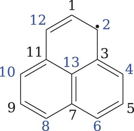
Figure 2. Spin-density distributions ${\rho }^{[-;1/2]}\left(\mathbf{r}\right)$ for the pristine phenalenyl computed for the doublet ground state obtained from (a) MCSCF, (b) UHF, (c) ROHF, (d) PBE50, (e) PBE0, (f) PBE, (g) TPSS calculations and (h) 2D structure with Mulliken populations (e) from the MCSCF calculation. Blue denotes positive spin-density and red denotes negative values. The isovalue is $\pm 0.001e\cdot {\text{Å}}^{-3}$ for positive and negative values, respectively.

The spin-distributions obtained with the MCSCF, UHF, and RHF methods as well as the PBE50, PBE0, PBE and TPSS functionals are displayed in Figure 2 for the pristine PLY. The wave functions were computed with $A_2$ symmetry within the $C_{2v}$ point group, but they display the full $A_1^{\mathrm{\prime }\mathrm{\prime }}$ symmetry within the $D_{3h}$ point group. Colour is used to distinguish between the regions of positive and negative spin-distributions. Blue is used to designate the α-rich positive regions, and red is used to designate the β-rich negative regions. All spin-distributions are computed with $M=+1/2$, thus the positive regions overall dominate the negative regions. The formal radical resides within the α-rich region, and additional spin-polarisation is reflected through the further positive and negative spin-distribution regions.

First considering the spin distribution for the pristine PLY (Figure 2), all methods present alternance of positive and negative spin densities on neighbouring carbons residing mostly in the π-system, a similar pattern as also seen for triangulene structures with larger number of rings [55]. The exception to this is the RHF result in Figure 2(c) which shows only positive spin-distribution values. As discussed in Section 2.2 this is the expected result for an RHF wave function with M>0. For the other methods, there are 7 α-rich and 6 β-rich sites, consistent with the starred and unstarred C atoms in the alternant hydrocarbon. The VB framework provides some insight into the spin distributions. Here, spin population on a position can be seen as the result of a weighted combination of the resonance structures presenting open radicals on that site. Enhanced positive spin (blue) is found for the seven positions that can hold the free radical in the VB picture as indicated in blue in Figure 1. As discussed above, the radical on the central atom does not allow the formation of a Clar sextet. Thus, this resonance structure should possess a higher energy and present a lower contribution to the spin distribution. This difference is clearly represented in the MCSCF results [Figure 2(a)] where the outer positions display a spin-density of about four times the value of the inner atom (0.252e vs. 0.068e). UHF [Figure 2(b)] displays a strikingly different spin-distribution, which is, first, significantly more pronounced than the MCSCF one and, second, shows a diminished difference between outer and inner atoms (0.784e vs. 0.724e). RHF [Figure 2(c)] presents the opposite limiting case with no spin-density in the centre. Proceeding to UKS, we find that reducing the amount of HFX in the functional along the series PBE50 (d), PBE0 (e), PBE (f) reduces the overall spin-density on the atoms and restores the difference between the outer and central carbon atoms. Finally, TPSS (g), which is a local meta-GGA based on PBE, provides a similar appearance to PBE. In agreement with Refs. [7, 8], we find that using little or no HFX tends to improve the results. Specifically, the Mulliken population analysis for the MCSCF and TPSS calculations differs by at most 0.0267e (Table S1), highlighting that TPSS is a suitable choice for the description of this molecule.

Figure 2 illustrates the challenges present in describing spin-densities using UHF/UKS approaches. Dramatic differences and qualitatively diverging results are observed between different functionals, and, were the MCSCF reference not available, there would be no simple way to assess the quality of these descriptions. From a more formal viewpoint it is worth noting that our GUGA-based MCSCF strictly produces spin-eigenfunctions. The negative spin-distributions seen in Figure 2(a) arise via electron correlation. By contrast, negative spin-distributions from a UHF/UKS single determinantal treatment can only arise via spin-contamination, i.e. the α and β spin-orbitals have different shapes and, as a consequence, the resulting determinant is no longer an eigenfunction of ${\hat{S}}^2$, (see the Appendix for further details). Following Equation (1(1) ${\hat{S}}^2|\psi ;S,M〉=S(S+1)|\psi ;S,M〉,$(1) ), the expectation value $〈{\hat{S}}^2〉$ for a doublet state should be 0.75, and the deviations from that value can be used to quantify the spin-contamination. Increasing the HFX, we find that spin-contamination increases sharply and, specifically, $〈{\hat{S}}^2〉$ values of 0.766 (PBE), 0.824 (PBE0), 0.973 (PBE50), and 2.01 (UHF) are obtained. Further discussions of spin-contamination in UKS theory are quite subtle [12, 56, 57] and outside the scope of this work, but two points are particularly relevant. First, the KS determinant is an auxiliary construction whose purpose is to produce values for charge and spin densities whereas its $〈{\hat{S}}^2〉$ expectation value does not have a physical meaning. There is no reason to expect that $〈{\hat{S}}^2〉$ would reflect the true spin of the system. Second, UHF, as a wave function theory, is required to produce a valid $〈{\hat{S}}^2〉$ expectation value, [Equations (A6(A6) $\begin{array}{rl}& 〈\mathrm{U}\mathrm{H}\mathrm{F};\ast ,M|{\hat{S}}^2|\mathrm{U}\mathrm{H}\mathrm{F};\ast ,M〉\\ & =M(M+1)+N_{\text{β}}-\sum _{p=1}^{N_{\alpha }}\sum _{q=1}^{N_{\text{β}}}{X}_{pq}^2,\end{array}$(A6) ) and (A15(A15) $〈\mathrm{U}\mathrm{H}\mathrm{F};\ast ,M|{\hat{S}}^2|\mathrm{U}\mathrm{H}\mathrm{F};\ast ,M〉=\sum _{S=S_{min}}^{S_{max}}{x}_S^2\left(S\right(S+1\left)\right).$(A15) )]. In this sense, the spin-contamination in UHF is more troublesome than in UKS. Therefore, UHF as such, and by extension its admixture to UKS within a hybrid functional, is more problematic than using the original ‘pure’ UKS theory. Hence, in line with the observed results, a pure functional seems more suitable than a hybrid functional for the description of spin-densities.

The RHF results in Figure 2(c) are consistent with an uncorrelated (single determinant in this case) spin-eigenfunction with spin-promotion index ${\mathrm{\Delta }}^{\left(1/2\right)}=0e$ in Equation (33(33) ${\mathrm{\Delta }}^{\left(M\right)}=min(p_{+}^{\left(M\right)},-p_{-}^{\left(M\right)}),$(33) ). The RHF spin-distribution arises only from the delocalisation of the SOMO, with no contributions either from electron correlation or from spin-contamination. The RHF SOMO has $a_2\left(a_1^{\mathrm{\prime }\mathrm{\prime }}\right)$ symmetry in the $C_{2v}\left(D_{3h}\right)$ point group. The central carbon atom lies at the intersection of three vertical nodal planes of the SOMO and therefore acquires no significant spin-distribution from this delocalisation. In contrast, this central carbon has significant positive spin-density due to correlation in the MCSCF wave function in Figure 2(a).

The NSDOs of the MCSCF wave function, the spin-promotion distributions, and the spin-promotion numbers for PLY are shown in Figure 3. The natural charge-density orbitals obtained from the MCSCF calculation are displayed in Table S2. The spin-promotion numbers $p_{+}^{\left(1/2\right)}=1.564e$ and $p_{-}^{\left(1/2\right)}=-0.564e$ are consistent with the $M=1/2$ value and with significant spin polarisation within the wave function. In addition to the nominal SOMO distribution, the spin-promotion index ${\mathrm{\Delta }}^{\left(1/2\right)}=0.564e$, Equation (33(33) ${\mathrm{\Delta }}^{\left(M\right)}=min(p_{+}^{\left(M\right)},-p_{-}^{\left(M\right)}),$(33) ), shows additional promotion from the negative spin-promotion distribution regions into the positive regions. Within the 13-orbital active space, the lowest six NSDOs have negative ${\mu }_p^{\left(1/2\right)}$ eigenvalues and the remaining seven NSDOs have positive eigenvalues. Both the NSDOs and the eigenvalues reflect the $D_{3h}$ point group symmetry of the molecule. The positive spin-promotion distribution is concentrated on the six alternating edge carbons, as suggested from the VB analysis, and also consistent with the delocalisation of the $a_1^{\mathrm{\prime }\mathrm{\prime }}$ SOMO. A smaller positive spin-promotion distribution occurs on the central carbon, a consequence of the valence correlation. This density does not arise from the SOMO, which has three intersecting vertical nodal planes centred on that atom. The smaller negative spin-promotion distribution is spread among the other three edge carbons and the remaining three carbons, consistent with their unstarred C-atom designations. Due to these spatial separations, there is relatively little cancellation of positive and negative spin-promotion distribution to form the total spin-distribution ${\rho }^{[-;1/2]}\left(\mathbf{r}\right)$ shown in Figure 2(a). The square of the orbital amplitude times the ${\mu }_p^{\left(1/2\right)}$ eigenvalue for each orbital gives the contribution of that orbital to the spin-promotion distribution. Thus all of the orbitals on the left in Figure 3 contribute only positive values and all of the orbitals on the right contribute only negative values to the respective spin-promotion distribution and to the total spin-distribution.

Figure 3. ${\rho }_{\pm }^{[-;1/2]}\left(\mathbf{r}\right)$ spin-promotion distributions and the natural spin-density orbitals (NSDOs) with their eigenvalues (${\mu }_p^{\left(1/2\right)}$) for the pristine phenalenyl computed for the ${}^2{A}_2\left({}^2{A}_1^{\mathrm{\prime }\mathrm{\prime }}\right)$ ground state obtained from the MCSCF calculation. The isovalue is $\pm 0.001e\cdot {\text{Å}}^{-3}$ for ${\rho }_{\pm }^{[-;1/2]}\left(\mathbf{r}\right)$ and $\pm 0.05{\text{Å}}^{-3/2}$ for the NSDOs. Blue and red represent positive and negative values, respectively.

The spin distributions for the N-doped structures are displayed in Figures 4 and 5. These substitutions are isoeletronic to PLY and lead to a pyridinic form, not affecting the number of electrons in the π-system of the molecule. These substitutions break the $D_{3h}$ symmetry of the molecule, reducing it to ${\mathrm{C}}_{2v}$ for the C₁₁N₂H₇ di-substitution and to $C_s$ for the C₁₂NH₈ mono-substitution.

Figure 4. Spin-density distributions ${\rho }^{[-;1/2]}\left(\mathbf{r}\right)$ for the N-didoped phenalenyl computed for the doublet ground state obtained from (a) MCSCF, (b) TPSS calculations and (c) 2D structure with Mulliken populations (e) from the MCSCF calculation. Blue denotes positive spin density and red denotes negative values. The isovalue is $\pm 0.001e\cdot {\text{Å}}^{-3}$ for positive and negative values, respectively.

Figure 5. Spin-density distributions ${\rho }^{[-;1/2]}\left(\mathbf{r}\right)$ for the N-monodoped phenalenyl computed for the doublet ground state obtained from (a) MCSCF, (b) TPSS calculations and (c) 2D structure with Mulliken populations (e) from the MCSCF calculation. Blue denotes positive spin density and red denotes negative values. The isovalue is $\pm 0.001e\cdot {\text{Å}}^{-3}$ for positive and negative values, respectively.

Concerning the spin distribution for the doping by two N atoms (Figure 4), there is no appreciable qualitative change in comparison to the pristine case. The MCSCF spin-promotion index is ${\mathrm{\Delta }}^{\left(1/2\right)}=0.552e$, which is comparable to the PLY value. For both the MCSCF and TPSS methods, based on the Mulliken analysis, the spin population decreases in position 2 of the molecule in comparison to PLY, from 0.25e to 0.21e for the MCSCF method and more drastically from 0.28e to 0.18e for the TPSS functional, as seen in Table S3. The natural charge-density orbitals and NSDOs calculated with the MCSCF method are displayed in Tables S4 and S5.

For the spin-density of the single N-doped structure (Figure 5), a comparison of the spin distribution obtained from the RAS(3)/CAS(7,7)/AUX(3) calculation with the pristine counterpart (Figure 2) shows that the MCSCF method predicts a slightly larger spin distribution on the nitrogen and central carbon atoms than the TPSS functional (Table S6). The former has values equal to 0.22e (N) and 0.07e (C) while the latter has values equal to 0.20e (N) and 0.02e (C). The MCSCF spin-promotion index is ${\mathrm{\Delta }}^{\left(1/2\right)}=0.560e$, which is comparable to the PLY value. The natural charge-density orbitals and NSDOs attained from the RAS(3)/CAS(7,7)/AUX(3) wavefunction are displayed in Tables S7 and S8.

Figure 6 shows the NH di-substitution structures. This molecule presents a $C_{2v}$ symmetry and adds two more electrons on the π-system, resulting in nine electrons in the complete active space, RAS(3)/CAS(9,7)/AUX(3). The SOMO for this wave function has $a_2$ symmetry, and the wave function itself has $A_2$ symmetry. The MCSCF spin-promotion index is ${\mathrm{\Delta }}^{\left(1/2\right)}=0.160e$, which is much less than the PLY value and the previous N-substitution values. Within the 13-orbital active space, the lowest five NSDOs have negative ${\mu }_p^{\left(1/2\right)}$ eigenvalues and the remaining eight NSDOs have positive eigenvalues. A spin-distribution closer to an ROHF wave function is observed in Figure 6. According to results obtained from highly correlated multireference methods, this graphitic doping is expected to have the potential of enhancing the biradicaloid character for larger polyaromatic hydrocarbons [58–62]. Moreover, among the doping possibilities considered here, this type of substitution is the only one that changes qualitatively the α and β alternance in neighbouring atoms (Figure 6). For both methods considered, 10 of the 12 edge atoms present α spin while only the carbons in position 1, 7 and 13 (central) present β spin. These carbon atoms lie in the vertical nodal plane of the $a_2$ SOMO, and thereby receive no significant spin-distribution from the delocalisation of this orbital. For the TPSS functional, a small β spin-distribution is also observed between the carbons (i.e. within the chemical bonds) presenting σ character. The RAS(3)/CAS(9,7)/AUX(3) wave function cannot validate these contributions since there are no σ orbitals in the active space. This feature will be examined in more detail in future work using more accurate wave functions. The spin population for this structure is listed in Table S9, and the MCSCF and the DFT values differ by no more than 0.024e. The natural charge-density orbitals and the NSDOs obtained from the RAS(3)/CAS(9,7)/AUX(3) method are displayed in Tables S10 and S11.

Figure 6. Spin-density distributions ${\rho }^{[-;1/2]}\left(\mathbf{r}\right)$ for the NH-didoped phenalenyl computed for the doublet ground state obtained from (a) MCSCF, (b) TPSS calculations and (c) 2D structure with Mulliken populations (e) from the MCSCF calculation. Blue denotes positive spin density and red denotes negative values. The isovalue is $\pm 0.001e\cdot {\text{Å}}^{-3}$ for positive and negative values, respectively.

4. Conclusion

In this work, the theoretical background for the spin-density matrix calculation is presented. The matrix equation is written in terms of one- and two-particle charge density matrix elements that do not depend on the spin component quantum number and are available within the GUGA formalism. This approach avoids the projection of the wave function in a basis of spin-dependent Slater determinants, and it uses information that is already computed and is available within the MCSCF optimisation procedure. This approach is also applicable to MRCI and MR-AQCC methods.

The properties of the spin-density matrix and its spatial spin-distribution are discussed. Among several insights, the spin-distribution for a wave function that is a spin-eigenfunction with M = 0 vanishes everywhere in space, while this is not true for spin-contaminated M = 0 wave functions. In the latter case, it is only the integral over all space that is zero. Moreover, $M\ne 0$ multiconfigurational wave functions that are spin-eigenfunctions are able to produce spin-distributions with both positive and negative regions due to electron correlation, in contrast to unrestricted wave functions in which this feature arises due to spin-contamination. The natural spin-density orbitals provide a convenient basis for the discussion of the spin-distributions. Spin-promotion distributions and spin-promotion numbers provide insight into the spin-polarisation of the MCSCF wave function.

The implementation of the spin-density matrix calculation for the MCSCF method in Columbus was applied to the phenalenyl benzenoid radical and three doped structures, substituting the CH group by the N-atom and NH group. The pristine phenalenyl structure presents alternating α- and β-rich regions on neighbouring carbons, as do the N-atom mono- and di-substituted radicals. These radicals all display comparable spin-polarisation. In contrast, the NH di-substituted radical does not show alternating regions, and it displays much smaller spin-polarisation.

When compared to DFT functionals, it is observed that UKS functionals with more Hartree-Fock exchange produce exaggerated spin-distributions, and by comparison with the MCSCF spin-distribution, a pure functional like TPSS is more reliable than hybrid functionals.

We believe this work provides solid basis on how to obtain spin properties from the multiconfigurational GUGA formalism and provides trustworthy tools to explore and shed light on the spin properties of molecular systems.

Acknowledgements

We are grateful for supply of computer time at the HPCC facilities of Texas Tech University. The authors also thank Lab-CCAM from ITA for computational resources.

Disclosure statement

The authors declare no conflict of interest.

Additional information

Funding

R.F.K.S. acknowleges support by Fundação de Amparo à Pesquisado Estado de Sào Paulo (FAPESP) [grant number 2019/07671-4], Conselho Nacional de Desenvolvimento Científico e Tecnológico (CNPq) [grant numbers 407760/2018-0 and 307846/2021-0]. M.P.F. was supported by Coordenação de Aperfeiçoamento de Pessoal de Nível Superior (CAPES) [grant number 88887.581913/2020-00]. R.S. was supported by the US Department of Energy (DOE), Office of Science, Basic Energy Sciences, Chemical Sciences, Geosciences, and Biosciences Division, Gas Phase Chemical Physics program through Argonne National Laboratory [contract DE-AC02-06CH11357]. H.L. wants to acknowledge support by the National Science Foundation [grant number 2107923], Division of Chemistry.

Appendix 1.

Spin-density matrices in UHF and UDFT formalism

In this appendix the formalism for UHF and UDFT spin-density matrix computation is briefly reviewed. The important feature of these methods is that a different-orbitals-for-different-spins (DODS) formulation is used rather than the same-orbital-for-different-spins (SODS) formulation that is employed within GUGA. These two sets of spatial orbitals will be denoted ${\mathit{\phi }}^{\left[\sigma \right]}$ with $\sigma \in \{\alpha ,\text{β}$}. These two sets of molecular orbitals are computed from the same set of atomic orbitals (AO) of dimension n, (A1) ${\mathit{\phi }}^{\left[\sigma \right]}=\mathit{\chi }{\mathbf{C}}^{\left[\sigma \right]}.$(A1) Let $\mathbf{X}$ be the overlap matrix between the two sets of spatial orbitals (A2) $X_{pq}=\int {\phi }_p^{\left[\alpha \right]}\left(\mathbf{r}{)}^{\ast }{\phi }_q^{\left[\text{β}\right]}\right(\mathbf{r})d\mathbf{r}\equiv 〈{\phi }_p^{\left[\alpha \right]},{\phi }_q^{\left[\text{β}\right]}〉,$(A2) that define the DODS spin-orbitals. It then follows that (A3) ${\mathit{\phi }}^{\left[\text{β}\right]}={\mathit{\phi }}^{\left[\alpha \right]}\mathbf{X},$(A3) and that the square matrix $\mathbf{X}$, which we assume herein to be real, is orthogonal, ${\mathbf{X}}^T\mathbf{X}=\mathbf{X}{\mathbf{X}}^T=\mathbf{1}$.

The UHF wave function consists of a simpler, single-determinant, form rather than the explicitly multiconfigurational form of the MCSCF wave functions used in the present work. The UHF orbitals are optimised to minimise the single-determinant energy expectation value, and the resulting wave function is an eigenfunction of the ${\hat{S}}_z$ operator, but it is typically not an eigenfunction of the ${\hat{S}}^2$ operator. Briefly, with a suitable ordering of the molecular orbitals the UHF determinant is written in the occupation number representation as (A4) $|\mathrm{U}\mathrm{H}\mathrm{F};\ast ,M〉=|\stackrel{n}{\overbrace{\underset{N_{\alpha }}{\underbrace{1\cdots 1}}0\cdots 0}}\stackrel{n}{\overbrace{\underset{N_{\text{β}}}{\underbrace{1\cdots 1}}0\cdots 0}}〉,$(A4) with the spin-orbital occupations ${\eta }_{k\sigma }\in \{0,1\}$. The spin-orbital basis has dimension $2n$. The first $N_{\alpha }$ of the α spin-orbitals are occupied, followed by the $n-N_{\alpha }$ unoccupied α spin-orbitals, followed by the first $N_{\text{β}}$ of the occupied β spin-orbitals, followed by the $n-N_{\text{β}}$ unoccupied β spin-orbitals. In the DODS basis, the ${\hat{S}}_z$ operator form is unchanged, while the ${\hat{S}}_{+}$ and ${\hat{S}}_{-}$ operators take the form (A5) $\begin{array}{rl}{\hat{S}}_z& =\frac{1}{2}({\hat{N}}_{\alpha }-{\hat{N}}_{\text{β}}),\\ {\hat{S}}_{+}& ={\hat{S}}_{-}^{†}=\sum _{pq}{X}_{pq}{\hat{a}}_{p\alpha }^{†}{\hat{a}}_{q\text{β}},\\ {\hat{S}}_{-}& ={\hat{S}}_{+}^{†}=\sum _{pq}{X}_{pq}^T{\hat{a}}_{p\text{β}}^{†}{\hat{a}}_{q\alpha },\end{array}$(A5) In the special case that $\mathbf{X}=\mathbf{1}$, the DODS basis becomes an SODS basis, and the operators in Equation (A5(A5) $\begin{array}{rl}{\hat{S}}_z& =\frac{1}{2}({\hat{N}}_{\alpha }-{\hat{N}}_{\text{β}}),\\ {\hat{S}}_{+}& ={\hat{S}}_{-}^{†}=\sum _{pq}{X}_{pq}{\hat{a}}_{p\alpha }^{†}{\hat{a}}_{q\text{β}},\\ {\hat{S}}_{-}& ={\hat{S}}_{+}^{†}=\sum _{pq}{X}_{pq}^T{\hat{a}}_{p\text{β}}^{†}{\hat{a}}_{q\alpha },\end{array}$(A5) ) reduce to the simpler forms of Equation (7(7) $\begin{array}{rl}{\hat{S}}_z& =\frac{1}{2}\sum _k({\hat{a}}_{k\alpha }^{†}{\hat{a}}_{k\alpha }-{\hat{a}}_{k\text{β}}^{†}{\hat{a}}_{k\text{β}})\\ & =\frac{1}{2}({\hat{N}}_{\alpha }-{\hat{N}}_{\text{β}})=\frac{1}{\sqrt{2}}\sum _k{\hat{T}}_{kk}^{1,0},\\ {\hat{S}}_{+}& ={\hat{S}}_{-}^{†}=\sum _k{\hat{a}}_{k\alpha }^{†}{\hat{a}}_{k\text{β}}=-\sum _k{\hat{T}}_{kk}^{1,1},\\ {\hat{S}}_{-}& ={\hat{S}}_{+}^{†}=\sum _k{\hat{a}}_{k\text{β}}^{†}{\hat{a}}_{k\alpha }=\sum _k{\hat{T}}_{kk}^{1,-1}.\end{array}$(7) ) with a single spatial orbital summation index. These operators lead to the simple expression [63] for the UHF ${\hat{S}}^2$ expectation value, (A6) $\begin{array}{rl}& 〈\mathrm{U}\mathrm{H}\mathrm{F};\ast ,M|{\hat{S}}^2|\mathrm{U}\mathrm{H}\mathrm{F};\ast ,M〉\\ & =M(M+1)+N_{\text{β}}-\sum _{p=1}^{N_{\alpha }}\sum _{q=1}^{N_{\text{β}}}{X}_{pq}^2,\end{array}$(A6) where for M>0 the last two terms together are regarded as a measure of the spin-contamination.

The UHF spin-density matrix is typically computed in the atomic orbital (AO) basis rather than the MO basis. To arrive at this formulation, consider the 1-RDMs that arise separately from the α and β spin-orbitals of a DODS wave function. (A7) $D_{qp}^{[\sigma ;M]}=〈\psi ;\ast ,M|{\hat{a}}_{p\sigma }^{†}{\hat{a}}_{q\sigma }|\psi ;\ast ,M〉.$(A7) These density matrices are symmetric, the eigenvalues satisfy $0\le {\mu }_k\le 1\mathrm{\forall }k$, and $Tr\left({\mathbf{D}}^{[\sigma ;M]}\right)=N_{\sigma }$. For a single-determinant UHF wave function, these density matrices are diagonal, (A8) ${\mathbf{D}}^{[\sigma ;M]}=\mathrm{d}\mathrm{i}\mathrm{a}\mathrm{g}({\eta }_{1\sigma },\dots ,{\eta }_{n\sigma })$(A8) with the orbital occupations ${\eta }_{k\sigma }$ shown in Equation (A4(A4) $|\mathrm{U}\mathrm{H}\mathrm{F};\ast ,M〉=|\stackrel{n}{\overbrace{\underset{N_{\alpha }}{\underbrace{1\cdots 1}}0\cdots 0}}\stackrel{n}{\overbrace{\underset{N_{\text{β}}}{\underbrace{1\cdots 1}}0\cdots 0}}〉,$(A4) ). The corresponding spatial electron distributions are given by (A9) $\begin{array}{rl}{\rho }^{[\sigma ;M]}\left(\mathbf{r}\right)& =\sum _{pq}{\phi }_q^{\left[\sigma \right]}\left(\mathbf{r}\right)D_{qp}^{[\sigma ;M]}{\phi }_p^{\left[\sigma \right]}(\mathbf{r}{)}^{\ast }\\ & ={\mathit{\phi }}^{\left[\sigma \right]}\left(\mathbf{r}\right){\mathbf{D}}^{[\sigma ;M]}{\mathit{\phi }}^{\left[\sigma \right]}(\mathbf{r}{)}^{†},\\ & =\sum _{\mu \nu }{\chi }_{\nu }\left(\mathbf{r}\right)D_{\nu \mu }^{[\sigma ;\chi ;M]}{\chi }_{\mu }(\mathbf{r}{)}^{\ast }=\mathit{\chi }(\mathbf{r}\left){\mathbf{D}}^{[\sigma ;\chi ;M]}\mathit{\chi }\right(\mathbf{r}{)}^{†},\end{array}$(A9) with the AO density matrices ${\mathbf{D}}^{[\sigma ;\chi ;M]}={\mathbf{C}}^{\left[\sigma \right]}{\mathbf{D}}^{[\sigma ;M]}{\mathbf{C}}^{\left[\sigma \right]T}$. Integration over all space of the spatial distributions gives, (A10) $\begin{array}{rl}\int {\rho }^{[\sigma ;M]}\left(\mathbf{r}\right)d\mathbf{r}& =\sum _{\mu \nu }{D}_{\nu \mu }^{[\sigma ;\chi ;M]}\int {\chi }_{\mu }\left(\mathbf{r}{)}^{\ast }{\chi }_{\nu }\right(\mathbf{r})d\mathbf{r}\\ & =\sum _{\mu \nu }{D}_{\nu \mu }^{[\sigma ;\chi ;M]}{S}_{\mu \nu }^{AO}\\ & =\mathrm{T}\mathrm{r}\left({\mathbf{D}}^{[\sigma ;\chi ;M]}{\mathbf{S}}^{AO}\right)=N_{\sigma }.\end{array}$(A10) In the common AO basis, the total charge density matrix ${\mathbf{D}}^{[+;\chi ;M]}$ and the spin-density matrix ${\mathbf{D}}^{[-;\chi ;M]}$ are (A11) ${\mathbf{D}}^{[\pm ;\chi ;M]}={\mathbf{D}}^{[\alpha ;\chi ;M]}\pm {\mathbf{D}}^{[\text{β};\chi ;M]}.$(A11) The total spatial charge distribution ${\rho }^{[+;M]}\left(\mathbf{r}\right)$ and the spatial spin-distribution ${\rho }^{[-;M]}\left(\mathbf{r}\right)$ are given by (A12) $\begin{array}{rl}{\rho }^{[\pm ;M]}\left(\mathbf{r}\right)& ={\rho }^{[\alpha ;M]}\left(\mathbf{r}\right)\pm {\rho }^{[\text{β};M]}\left(\mathbf{r}\right)\\ & =\sum _{\mu \nu }{\chi }_{\nu }\left(\mathbf{r}\right)D_{\nu \mu }^{[\pm ;\chi ;M]}{\chi }_{\mu }(\mathbf{r}{)}^{\ast }=\mathit{\chi }(\mathbf{r}\left){\mathbf{D}}^{[\pm ;\chi ;M]}\mathit{\chi }\right(\mathbf{r}{)}^{†}.\end{array}$(A12) It follows from Equation (A10(A10) $\begin{array}{rl}\int {\rho }^{[\sigma ;M]}\left(\mathbf{r}\right)d\mathbf{r}& =\sum _{\mu \nu }{D}_{\nu \mu }^{[\sigma ;\chi ;M]}\int {\chi }_{\mu }\left(\mathbf{r}{)}^{\ast }{\chi }_{\nu }\right(\mathbf{r})d\mathbf{r}\\ & =\sum _{\mu \nu }{D}_{\nu \mu }^{[\sigma ;\chi ;M]}{S}_{\mu \nu }^{AO}\\ & =\mathrm{T}\mathrm{r}\left({\mathbf{D}}^{[\sigma ;\chi ;M]}{\mathbf{S}}^{AO}\right)=N_{\sigma }.\end{array}$(A10) ) that integration over space gives, (A13) $\int {\rho }^{[\pm ;M]}\left(\mathbf{r}\right)d\mathbf{r}=N_{\alpha }\pm N_{\text{β}}.$(A13) Because the UHF wave function is usually spin-contaminated, different values for the quantum number M correspond to distinct, energy-optimised, spin-contaminated wave functions, and they are not necessarily related to each other through ${\hat{S}}_{\pm }$ or through simple spin-tensor relations such as Equation (6(6) $\begin{array}{rl}({\hat{T}}_{pq}^{S,M}{)}^{†}& =(-1{)}^M{\hat{T}}_{qp}^{S,-M},\\ [{\hat{S}}_{\pm },{\hat{T}}_{pq}^{S,M}]& =\sqrt{S(S+1)-M(M\pm 1)}{\hat{T}}_{pq}^{S,M\pm 1},\\ [{\hat{S}}_z,{\hat{T}}_{pq}^{S,M}]& =M{\hat{T}}_{pq}^{S,M}.\end{array}$(6) ).

Another important difference between spin-eigenfunctions and spin-contaminated wave functions is that typically ${\mathbf{D}}^{[-;\chi ;0]}\ne \mathbf{0}$, for M = 0, in contrast to Equation (22(22) $D_{qp}^{(1,0;M)}=\frac{M}{S}{D}_{qp}^{(1,0;S)}.$(22) ). In principle, a spin-contaminated wave function may be expanded in a spin-eigenfunction basis, (A14) $|\psi ;\ast ,M〉=\sum _{S=S_{min}}^{S_{max}}{x}_S|\psi ;S,M〉,$(A14) with $S_{min}=|M|$ and $S_{max}=min(\frac{1}{2}N,n-\frac{1}{2}N)$. This expansion is discussed in more detail in Ref. [64]. In general, the spin-eigenfunction basis functions $|\psi ;S,M〉$ are multi-determinantal expansions in the DODS spin-orbital basis, even when the wave function $|\psi ;\ast ,M〉$ is a single UHF determinant. In terms of this expansion, the UHF ${\hat{S}}^2$ expectation value Equation (A6(A6) $\begin{array}{rl}& 〈\mathrm{U}\mathrm{H}\mathrm{F};\ast ,M|{\hat{S}}^2|\mathrm{U}\mathrm{H}\mathrm{F};\ast ,M〉\\ & =M(M+1)+N_{\text{β}}-\sum _{p=1}^{N_{\alpha }}\sum _{q=1}^{N_{\text{β}}}{X}_{pq}^2,\end{array}$(A6) ) is (A15) $〈\mathrm{U}\mathrm{H}\mathrm{F};\ast ,M|{\hat{S}}^2|\mathrm{U}\mathrm{H}\mathrm{F};\ast ,M〉=\sum _{S=S_{min}}^{S_{max}}{x}_S^2\left(S\right(S+1\left)\right).$(A15) The $S=|M|$ term in this expansion is typically the desired wave function, and any other nonzero terms, each of which is positive so there are no cancellations within the summation, are regarded as spin-contamination.

For a DODS wave function expansion, the spin-density operator in the ${\mathit{\phi }}^{\left[\alpha \right]}$ orbital basis may be written (A16) ${\hat{D}}_{qp}^{1,0}={\hat{a}}_{p\alpha }^{†}{\hat{a}}_{q\alpha }-\sum _{rs}{X}_{pr}{X}_{qs}{\hat{a}}_{r\text{β}}^{†}{\hat{a}}_{s\text{β}}.$(A16) This operator, along with its counterpart operator in the ${\mathit{\phi }}^{\left[\text{β}\right]}$ basis, is consistent with the AO spin-density matrix ${\mathbf{D}}^{[-;\chi ;M]}$ in Equation (A11(A11) ${\mathbf{D}}^{[\pm ;\chi ;M]}={\mathbf{D}}^{[\alpha ;\chi ;M]}\pm {\mathbf{D}}^{[\text{β};\chi ;M]}.$(A11) ). The expectation value of this operator then simplifies as (A17) $\begin{array}{rl}& 〈\psi ;\ast ,M|{\hat{D}}_{qp}^{1,0}|\psi ;\ast ,M〉\\ & =\sum _{S,S^{\mathrm{\prime }}}{x}_S{x}_{S^{\mathrm{\prime }}}〈\psi ;S,M|{\hat{D}}_{qp}^{1,0}|\psi ;S^{\mathrm{\prime }},M〉\end{array}$(A17) (A18) $\begin{array}{rl}& =\sum _{S=S_{min}}^{S_{max}}{x}_S^2〈\psi ;S,M|{\hat{D}}_{qp}^{1,0}|\psi ;S,M〉\\ & +\sum _{S=S_{min}}^{S_{max}-1}{x}_S{x}_{S+1}〈\psi ;S,M|{\hat{D}}_{qp}^{1,0}|\psi ;S+1,M〉\\ & +\sum _{S=S_{min}+1}^{S_{max}}{x}_S{x}_{S-1}〈\psi ;S,M|{\hat{D}}_{qp}^{1,0}|\psi ;S-1,M〉\end{array}$(A18) (A19) $\begin{array}{rl}& =\sum _{S=S_{min}}^{S_{max}}{x}_S^2〈\psi ;S,M|{\hat{D}}_{qp}^{1,0}|\psi ;S,M〉\\ & +\sum _{S=S_{min}}^{S_{max}-1}{x}_S{x}_{S+1}〈\psi ;S,M|{\hat{D}}_{qp}^{1,0}+{\hat{D}}_{pq}^{1,0}|\psi ;S+1,M〉,\end{array}$(A19) due to the triangle inequality constraints on the values $(S,S^{\mathrm{\prime }},1)$. In the spin-eigenfunction expansion basis, the first summation term in Equation (A18(A18) $\begin{array}{rl}& =\sum _{S=S_{min}}^{S_{max}}{x}_S^2〈\psi ;S,M|{\hat{D}}_{qp}^{1,0}|\psi ;S,M〉\\ & +\sum _{S=S_{min}}^{S_{max}-1}{x}_S{x}_{S+1}〈\psi ;S,M|{\hat{D}}_{qp}^{1,0}|\psi ;S+1,M〉\\ & +\sum _{S=S_{min}+1}^{S_{max}}{x}_S{x}_{S-1}〈\psi ;S,M|{\hat{D}}_{qp}^{1,0}|\psi ;S-1,M〉\end{array}$(A18) ) consists of the diagonal matrix elements, the second term consists of upper codiagonal elements, and the last term consists of lower codiagonal elements of a tridiagonal matrix. The last summation in Equation (A19(A19) $\begin{array}{rl}& =\sum _{S=S_{min}}^{S_{max}}{x}_S^2〈\psi ;S,M|{\hat{D}}_{qp}^{1,0}|\psi ;S,M〉\\ & +\sum _{S=S_{min}}^{S_{max}-1}{x}_S{x}_{S+1}〈\psi ;S,M|{\hat{D}}_{qp}^{1,0}+{\hat{D}}_{pq}^{1,0}|\psi ;S+1,M〉,\end{array}$(A19) ) follows from the identity $({\hat{D}}_{qp}^{1,0}{)}^{†}={\hat{D}}_{pq}^{1,0}$. If $S=|M|$ is the wave function of interest, then any nonzero $S\ne |M|$ terms in the first summation in Equation (A19(A19) $\begin{array}{rl}& =\sum _{S=S_{min}}^{S_{max}}{x}_S^2〈\psi ;S,M|{\hat{D}}_{qp}^{1,0}|\psi ;S,M〉\\ & +\sum _{S=S_{min}}^{S_{max}-1}{x}_S{x}_{S+1}〈\psi ;S,M|{\hat{D}}_{qp}^{1,0}+{\hat{D}}_{pq}^{1,0}|\psi ;S+1,M〉,\end{array}$(A19) ) and the entire contribution of the second summation would be considered spin-contamination. For M = 0 the first summation in Equation (A19(A19) $\begin{array}{rl}& =\sum _{S=S_{min}}^{S_{max}}{x}_S^2〈\psi ;S,M|{\hat{D}}_{qp}^{1,0}|\psi ;S,M〉\\ & +\sum _{S=S_{min}}^{S_{max}-1}{x}_S{x}_{S+1}〈\psi ;S,M|{\hat{D}}_{qp}^{1,0}+{\hat{D}}_{pq}^{1,0}|\psi ;S+1,M〉,\end{array}$(A19) ) vanishes due to Equation (22(22) $D_{qp}^{(1,0;M)}=\frac{M}{S}{D}_{qp}^{(1,0;S)}.$(22) ) to give, (A20) $\begin{array}{rl}& 〈\psi ;\ast ,0|{\hat{D}}_{qp}^{1,0}|\psi ;\ast ,0〉\\ & =\sum _{S=0}^{S_{max}-1}{x}_S{x}_{S+1}〈\psi ;S,0|{\hat{D}}_{qp}^{1,0}+{\hat{D}}_{pq}^{1,0}|\psi ;S+1,0〉.\end{array}$(A20) These spin-density matrix elements are composed entirely of spin-contamination contributions from off-diagonal adjacent terms in the spin-eigenfunction expansion. The nonzero eigenvalues of this matrix must be both positive and negative in order to satisfy $\mathrm{T}\mathrm{r}\left({\mathbf{D}}^{(1,0;M)}\right)=2M=0$, and thus a nonzero spatial spin-distribution at some point $\mathbf{r}$ in space can be either positive or negative, with integration over all space giving zero. The possibility of a nonzero spatial spin-distribution is also apparent from Equation (A12(A12) $\begin{array}{rl}{\rho }^{[\pm ;M]}\left(\mathbf{r}\right)& ={\rho }^{[\alpha ;M]}\left(\mathbf{r}\right)\pm {\rho }^{[\text{β};M]}\left(\mathbf{r}\right)\\ & =\sum _{\mu \nu }{\chi }_{\nu }\left(\mathbf{r}\right)D_{\nu \mu }^{[\pm ;\chi ;M]}{\chi }_{\mu }(\mathbf{r}{)}^{\ast }=\mathit{\chi }(\mathbf{r}\left){\mathbf{D}}^{[\pm ;\chi ;M]}\mathit{\chi }\right(\mathbf{r}{)}^{†}.\end{array}$(A12) ). This is in contrast to the M = 0 spin-distribution for a wave function that is a spin-eigenfunction, which vanishes at every point in space, Equation (25(25) $\begin{array}{rl}{\rho }^{[-;M]}\left(\mathbf{r}\right)& ={\rho }^{[\alpha ;M]}\left(\mathbf{r}\right)-{\rho }^{[\text{β};M]}\left(\mathbf{r}\right)\\ & =\sum _{pq}{\phi }_q\left(\mathbf{r}\right)D_{qp}^{(1,0;M)}{\phi }_p(\mathbf{r}{)}^{\ast }\\ & =\mathit{\phi }\left(\mathbf{r}\right){\mathbf{D}}^{(1,0;M)}\mathit{\phi }(\mathbf{r}{)}^{†}\\ & =\frac{M}{S}{\rho }^{[-;S]}\left(\mathbf{r}\right).\end{array}$(25) ).

References

- I. Shavitt, Int. J. Quantum Chem. 12(S11), 131–148 (2009). doi:10.1002/qua.v12:11+
- I. Shavitt, Int. J. Quantum Chem. 14(S12), 5–32 (2009). doi:10.1002/qua.v14:12+
- I. Shavitt, in The Unitary Group for the Evaluation of Electronic Energy Matrix Elements: Unitary Group Workshop 1979, Lecture Notes in Chemistry Vol. 22, edited by J. Hinze (Springer-Verlag, Berlin, 1981), pp. 51–99.
- J. Paldus, J. Chem. Phys. 61(12), 5321–5330 (1974). doi:10.1063/1.1681883
- H. Lischka, R. Shepard, T. Müller, P.G. Szalay, R.M. Pitzer, A.J.A. Aquino, M.M. Araújo do Nascimento, M. Barbatti, L.T. Belcher, J.P. Blaudeau, I. Borges, S.R. Brozell, E.A. Carter, A. Das, G. Gidofalvi, L. González, W.L. Hase, G. Kedziora, M. Kertesz, F. Kossoski, F.B.C. Machado, S. Matsika, S.A. do Monte, D. Nachtigallová, R. Nieman, M. Oppel, C.A. Parish, F. Plasser, R.F.K. Spada, E.A. Stahlberg, E. Ventura, D.R. Yarkony and Z. Zhang, J. Chem. Phys. 152(13), 134110 (2020). doi:10.1063/1.5144267
- E. Ruiz, J. Cirera and S. Alvarez, Coord. Chem. Rev. 249(23), 2649–2660 (2005). doi:10.1016/j.ccr.2005.04.010
- M. Radon, E. Broclawik and K. Pierloot, J. Phys. Chem. B 114(3), 1518–1528 (2010). doi:10.1021/jp910220r
- K. Boguslawski, K.H. Marti, O. Legeza and M. Reiher, J. Chem. Theory Comput. 8(6), 1970–1982 (2012). doi:10.1021/ct300211j
- F. Plasser, S.A. Bäppler, M. Wormit and A. Dreuw, J. Chem. Phys. 141(2), 024107 (2014). doi:10.1063/1.4885820
- R. McWeeny, Spins in Chemistry (Courier Corporation, New York, 2004).
- A. Schweiger and G. Jeschke, Principles of Pulse Electron Paramagnetic Resonance (Oxford University Press on Demand, New York, 2001).
- C.R. Jacob and M. Reiher, Int. J. Quantum Chem. 112(23), 3661–3684 (2012). doi:10.1002/qua.24309
- M.L. Munzarová, B. Engels, V.A. Rassolov, D.M. Chipman, S. Patchkovskii, G. Schreckenbach, G.H. Lushington and F. Neese, in Calculation of NMR and EPR Parameters: Theory and Applications, edited by M. Kaupp, M. Bühl and V.G. Malkin (Wiley-VCH, Weinheim, Germany, 2004), pp. 461–564.
- F. Rastrelli and A. Bagno, Chem. Eur. J. 15(32), 7990–8004 (2009). doi:10.1002/chem.v15:32
- J. Autschbach, S. Patchkovskii and B. Pritchard, J. Chem. Theory Comput. 7(7), 2175–2188 (2011). doi:10.1021/ct200143w
- F. Aquino, B. Pritchard and J. Autschbach, J. Chem. Theory Comput. 8(2), 598–609 (2012). doi:10.1021/ct2008507
- M. Radon and K. Pierloot, J. Phys. Chem. A 112(46), 11824–11832 (2008). doi:10.1021/jp806075b
- A. Ghosh, J. Biol. Inorg. Chem. 11(6), 712–724 (2006). doi:10.1007/s00775-006-0135-4
- J. Conradie and A. Ghosh, J. Phys. Chem. B 111(44), 12621–12624 (2007). doi:10.1021/jp074480t
- U. Von Barth and L. Hedin, J. Phys. C: Solid State Phys. 5(13), 1629– 1642 (1972). doi:10.1088/0022-3719/5/13/012
- H. Lischka, T. Müller, P.G. Szalay, I. Shavitt, R.M. Pitzer and R. Shepard, WIRES 1, 191–199 (2011). doi:10.1002/wcms.25
- H. Lischka, R. Shepard, R. M. Pitzer, I. Shavitt, M. Dallos, T. Müller, P.G. Szalay, M. Seth, G. S. Kedziora, S. Yabushita and Z. Zhang, Phys. Chem. Chem. Phys. 3(5), 664–673 (2001). doi:10.1039/b008063m
- H. Lischka, R. Shepard, I. Shavitt, R.M. Pitzer, T. Müller, P.G. Szalay, S.R. Brozell, G. Kedziora, E.A. Stahlberg, R.J. Harrison, J. Nieplocha, M. Minkoff, M. Barbatti, M. Schuurmann, Y. Guan, D.R. Yarkony, S. Matsika, F. Plasser, E.V. Beck, J.P. Blaudeau, M. Ruckenbauer, B. Sellner, J.J. Szymczak, R.F.K. Spada, A. Das, L.T. Belcher and R. Nieman, Columbus, an ab initio electronic structure program, release 7.0, https://www.univie.ac.at/columbus/ (2021).
- Z.H. Cui, H. Lischka, H.Z. Beneberu and M. Kertesz, J. Am. Chem. Soc. 136(15), 5539–5542 (2014). doi:10.1021/ja412862n
- A. Das, T. Müller, F. Plasser and H. Lischka, J. Phys. Chem. A 120(9), 1625–1636 (2016). doi:10.1021/acs.jpca.5b12393
- T. Kubo and K. Uchida, J. Synth. Org. Chem. Jpn. 74, 1067–1077 (2016). doi:10.5059/yukigoseikyokaishi.74.1069
- Z.D. Levey, B.A. Laws, S.P. Sundar, K. Nauta, S.H. Kable, G. da Silva, J.F. Stanton and T.W. Schmidt, J. Phys. Chem. A 126(1), 101–108 (2022). doi:10.1021/acs.jpca.1c08310
- Y. Morita, S. Suzuki, K. Fukui, S. Nakazawa, H. Kitagawa, H. Kishida, H. Okamoto, A. Naito, A. Sekine, Y. Ohashi, M. Shiro, K. Sasaki, D. Shiomi, K. Sato, T. Takui and K. Nakasuji, Nat. Mater. 7(1), 48–51 (2008). doi:10.1038/nmat2067
- Y. Morita, S. Suzuki, K. Sato and T. Takui, Nat. Chem. 3(3), 197–204 (2011). doi:10.1038/nchem.985
- K. Tagami, L. Wang and M. Tsukada, Nano Lett. 4(2), 209–212 (2004). doi:10.1021/nl0348894
- H. Wei, Y. Liu, T.Y. Gopalakrishna, H. Phan, X. Huang, L. Bao, J. Guo, J. Zhou, S. Luo, J. Wu and Z. Zeng, J. Am. Chem. Soc. 139(44), 15760–15767 (2017). doi:10.1021/jacs.7b07375
- P. De Silva, J. Phys. Chem. Lett. 10(18), 5674–5679 (2019). doi:10.1021/acs.jpclett.9b02333
- R. Pauncz, Spin Eigenfunctions: Construction and Use (1979). New York: Plenum Press.
- D.M. Brink and G.K. Sactchler, Angular Momentum (Clarendon Press, Oxford, Glasgow, 1968).
- T. Helgaker, P. Jorgensen and J. Olsen, Molecular Electronic Structure Theory (John Wiley & Sons Ltd, Chichester, 2000).
- F.A. Matsen, Int. J. Quantum Chem. 10(3), 525–542 (1976). doi:10.1002/(ISSN)1097-461X
- E. Wigner, Z. Phys. 43(9-10), 624–652 (1927). doi:10.1007/BF01397327
- C. Eckart, Rev. Mod. Phys. 2(3), 305–380 (1930). doi:10.1103/RevModPhys.2.305
- G. Gidofalvi and R. Shepard, Int. J. Quantum Chem. 109(15), 3552–3563 (2009). doi:10.1002/qua.v109:15
- F. Aquilante, J. Autschbach, R.K. Carlson, L.F. Chibotaru, M.G. Delcey, L. De Vico, I.F. Galván, N. Ferré, L.M. Frutos, L. Gagliardi, M. Garavelli, A. Giussani, C.E. Hoyer, G. Li Manni, H. Lischka, D. Ma, P.A. Malmqvist, T. Müller, A. Nenov, M. Olivucci, T.B. Pedersen, D. Peng, F. Plasser, B. Pritchard, M. Reiher, I. Rivalta, I. Schapiro, J. Segarrá Martí, M. Stenrup, D.G. Truhlar, L. Ungur, A. Valentini, S. Vancoillie, V. Veryazov, V.P. Vysotskiy, O. Weingart, F. Zapata, R. Lindh, J. Comput. Chem. 37, 506–541 (2016). doi:10.1002/jcc.v37.5
- P.G. Szalay, T. Muller, G. Gidofalvi, H. Lischka and R. Shepard, Chem. Rev. 112(1), 108–181 (2012). doi:10.1021/cr200137a
- F. Plasser, M. Wormit and A. Dreuw, J. Chem. Phys. 141(2), 024106 (2014). doi:10.1063/1.4885819
- M. Head-Gordon, A.M. Grana, D. Maurice and C.A. White, J. Phys. Chem. 99(39), 14261–14270 (1995). doi:10.1021/j100039a012
- R. Shepard, J. Phys. Chem. A 109(50), 11629–11641 (2005). doi:10.1021/jp0543431
- S.R. Brozell and R. Shepard, Mol. Phys. 119(21-22), e1950858 (2021). doi:10.1080/00268976.2021.1950858
- J. Tao, J.P. Perdew, V.N. Staroverov and G.E. Scuseria, Phys. Rev. Lett. 91(14), 3–6 (2003). doi:10.1103/PhysRevLett.91.146401
- F. Weigend and R. Ahlrichs, Phys. Chem. Chem. Phys. 7, 3297 (2005). doi:10.1039/b508541a
- F. Neese, WIREs Comput. Mol. Sci. 2(1), 73–78 (2012). doi:10.1002/wcms.v2.1
- R. Krishnan, J.S. Binkley, R. Seeger and J.A. Pople, J. Chem. Phys. 72(1), 650–654 (1980). doi:10.1063/1.438955
- J.P. Perdew, K. Burke and M. Ernzerhof, Phys. Rev. Lett. 77(18), 3865–3868 (1996). doi:10.1103/PhysRevLett.77.3865
- C. Adamo and V. Barone, J. Chem. Phys. 110(13), 6158–6170 (1999). doi:10.1063/1.478522
- Evgeny Epifanovsky, Andrew T. B. Gilbert, Xintian Feng, Joonho Lee, Yuezhi Mao, Narbe Mardirossian, Pavel Pokhilko, Alec F. White, Marc P. Coons, Adrian L. Dempwolff, Zhengting Gan, Diptarka Hait, Paul R. Horn, Leif D. Jacobson, Ilya Kaliman, Jörg Kussmann, Adrian W. Lange, Ka Un Lao, Daniel S. Levine, Jie Liu, Simon C. McKenzie, Adrian F. Morrison, Kaushik D. Nanda, Felix Plasser, Dirk R. Rehn, Marta L. Vidal, Zhi-Qiang You, Ying Zhu, Bushra Alam, Benjamin J. Albrecht, Abdulrahman Aldossary, Ethan Alguire, Josefine H. Andersen, Vishikh Athavale, Dennis Barton, Khadiza Begam, Andrew Behn, Nicole Bellonzi, Yves A. Bernard, Eric J. Berquist, Hugh G. A. Burton, Abel Carreras, Kevin Carter-Fenk, Romit Chakraborty, Alan D. Chien, Kristina D. Closser, Vale Cofer-Shabica, Saswata Dasgupta, Marc de Wergifosse, Jia Deng, Michael Diedenhofen, Hainam Do, Sebastian Ehlert, Po-Tung Fang, Shervin Fatehi, Qingguo Feng, Triet Friedhoff, James Gayvert, Qinghui Ge, Gergely Gidofalvi, Matthew Goldey, Joe Gomes, Cristina E. González-Espinoza, Sahil Gulania, Anastasia O. Gunina, Magnus W. D. Hanson-Heine, Phillip H. P. Harbach, Andreas Hauser, Michael F. Herbst, Mario Hernández Vera, Manuel Hodecker, Zachary C. Holden, Shannon Houck, Xunkun Huang, Kerwin Hui, Bang C. Huynh, Maxim Ivanov, Ádám Jász, Hyunjun Ji, Hanjie Jiang, Benjamin Kaduk, Sven Kähler, Kirill Khistyaev, Jaehoon Kim, Gergely Kis, Phil Klunzinger, Zsuzsanna Koczor-Benda, Joong Hoon Koh, Dimitri Kosenkov, Laura Koulias, Tim Kowalczyk, Caroline M. Krauter, Karl Kue, Alexander Kunitsa, Thomas Kus, István Ladjánszki, Arie Landau, Keith V. Lawler, Daniel Lefrancois, Susi Lehtola, Run R. Li, Yi-Pei Li, Jiashu Liang, Marcus Liebenthal, Hung-Hsuan Lin, You-Sheng Lin, Fenglai Liu, Kuan-Yu Liu, Matthias Loipersberger, Arne Luenser, Aaditya Manjanath, Prashant Manohar, Erum Mansoor, Sam F. Manzer, Shan-Ping Mao, Aleksandr V. Marenich, Thomas Markovich, Stephen Mason, Simon A. Maurer, Peter F. McLaughlin, Maximilian F. S. J. Menger, Jan-Michael Mewes, Stefanie A. Mewes, Pierpaolo Morgante, J. Wayne Mullinax, Katherine J. Oosterbaan, Garrette Paran, Alexander C. Paul, Suranjan K. Paul, Fabijan Pavošević, Zheng Pei, Stefan Prager, Emil I. Proynov, Ádám Rák, Eloy Ramos-Cordoba, Bhaskar Rana, Alan E. Rask, Adam Rettig, Ryan M. Richard, Fazle Rob, Elliot Rossomme, Tarek Scheele, Maximilian Scheurer, Matthias Schneider, Nickolai Sergueev, Shaama M. Sharada, Wojciech Skomorowski, David W. Small, Christopher J. Stein, Yu-Chuan Su, Eric J. Sundstrom, Zhen Tao, Jonathan Thirman, Gábor J. Tornai, Takashi Tsuchimochi, Norm M. Tubman, Srimukh Prasad Veccham, Oleg Vydrov, Jan Wenzel, Jon Witte, Atsushi Yamada, Kun Yao, Sina Yeganeh, Shane R. Yost, Alexander Zech, Igor Ying Zhang, Xing Zhang, Yu Zhang, Dmitry Zuev, Alán Aspuru-Guzik, Alexis T. Bell, Nicholas A. Besley, Ksenia B. Bravaya, Bernard R. Brooks, David Casanova, Jeng-Da Chai, Sonia Coriani, Christopher J. Cramer, György Cserey, A. Eugene DePrince III, Robert A. DiStasio Jr., Andreas Dreuw, Barry D. Dunietz, Thomas R. Furlani, William A. Goddard III, Sharon Hammes-Schiffer, Teresa Head-Gordon, Warren J. Hehre, Chao-Ping Hsu, Thomas-C. Jagau, Yousung Jung, Andreas Klamt, Jing Kong, Daniel S. Lambrecht, WanZhen Liang, Nicholas J. Mayhall, C. William McCurdy, Jeffrey B. Neaton, Christian Ochsenfeld, John A. Parkhill, Roberto Peverati, Vitaly A. Rassolov, Yihan Shao, Lyudmila V. Slipchenko, Tim Stauch, Ryan P. Steele, Joseph E. Subotnik, Alex J. W. Thom, Alexandre Tkatchenko, Donald G. Truhlar, Troy Van Voorhis, Tomasz A. Wesolowski, K. Birgitta Whaley, H. Lee Woodcock III, Paul M. Zimmerman, Shirin Faraji, Peter M. W. Gill, Martin Head-Gordon, John M. Herbert, and Anna I. Krylov, J. Chem. Phys. 155(8), 084801 (2021). doi:10.1063/5.0055522
- F. Plasser, A.I. Krylov and A. Dreuw, WIREs Comput. Mol. Sci. e1595 (2022). doi:10.1002/wcms.1595
- R. Pauncz, Alternant Molecular Orbital Method (Saunders, Philadelphia, 1967).
- A.M. Toader, C.M. Buta, B. Frecus, A. Mischie and F. Cimpoesu, J. Phys. Chem. C 123(11), 6869–6880 (2019). doi:10.1021/acs.jpcc.8b12250
- C.J. Cramer and D.G. Truhlar, Phys. Chem. Chem. Phys. 11(46), 10757 (2009). doi:10.1039/b907148b
- J.P. Perdew, A. Ruzsinszky, L.A. Constantin, J. Sun and G.I. Csonka, J. Chem. Theory Comput. 5(4), 902–908 (2009). doi:10.1021/ct800531s
- A. Das, T. Müller, F. Plasser, D.B. Krisiloff, E.A. Carter and H. Lischka, J. Chem. Theory Comput. 13(6), 2612–2622 (2017). doi:10.1021/acs.jctc.7b00156
- M. Pinheiro, L.F. Ferrao, F. Bettanin, A.J. Aquino, F.B. Machado and H. Lischka, Phys. Chem. Chem. Phys. 19(29), 19225–19233 (2017). doi:10.1039/C7CP03198J
- A. Das, M. Pinheiro Jr., F.B. Machado, A.J. Aquino and H. Lischka, ChemPhysChem 19(19), 2492–2499 (2018). doi:10.1002/cphc.201800650
- R. Nieman, N.J. Silva, A.J. Aquino, M.M. Haley and H. Lischka, J. Org. Chem. 85(5), 3664–3675 (2020). doi:10.1021/acs.joc.9b03308
- X. Shao, A.J. Aquino, M. Otyepka, D. Nachtigallová and H. Lischka, Phys. Chem. Chem. Phys. 22(38), 22003–22015 (2020). doi:10.1039/D0CP02688C
- A. Szabo and N.S. Ostlund, Modern Quantum Chemistry: Introduction to Advanced Electronic Structure Theory (Mineola, Dover, 1996).
- R. Shepard, Mol. Phys. (2022). Doi: 10.1080/00268976.2022.2077853