Interactions in coinage-metal/ligand complexes, CM–L, and their cations (CM = Cu, Ag, Au; L = CO, N₂ and H₂)

Abstract

The CM–L and CM⁺–L complexes for the three coinage metals, CM = Cu, Ag and Au interacting with three key ligands, L = CO, N₂ and H₂, are investigated. Calculations are undertaken using various quantum chemical methods to ascertain the equilibrium geometries and interaction energies; the latter are calculated at the coupled-cluster level of theory, and extrapolated to the basis set limit. Some of the neutral species are found to be particularly challenging, and significant disparity is found in some cases for the geometry and/or harmonic vibrational wavenumbers. In addition, molecular orbital diagrams, atomic charges, and orbital contour plots are presented, in order to gain insight into the interactions occurring in these complexes.

GRAPHICAL ABSTRACT

KEYWORDS:

• Coinage metals
• interaction energies of complexes
• carbon monoxide
• nitrogen
• hydrogen

1. Introduction

As well as underpinning an understanding of fundamental chemical interactions, a detailed understanding of single-atom catalysts will be aided by a knowledge of the interaction of reactant molecules with the deposited metal atoms. In reality, of course, the electronic structure, and so effective charge, of the metal atoms will be affected by the substrate [1–4]; hence, a full understanding of the catalytic activity is challenging. Density functional theory (DFT) is a relatively inexpensive computational method to employ to study such systems, but different functionals have been found to give disparate results for different systems. In the present work, as well as comparing to more-sophisticated quantum chemical methods, we will explore MP2, together with DFT employing three different functionals (B3LYP, CAM-B3LYP and PW91), to assess how consistent these are in establishing the equilibrium geometry of complexes formed between each of three ligands interacting with isolated coinage metal atoms, CM = Cu, Ag and Au, and their corresponding singly-charged atomic cations, CM⁺. The three ligands selected are CO, N₂, and H₂. As well as determining the global energy minima for the CM⁽⁺⁾–L complexes, we were interested in establishing the rationales for the binding motifs; in particular, the key differences between N₂ and CO – which are both isoelectronic and isobaric, and whose highest-occupied molecular orbitals (HOMOs) both have majority contributions from the 2p orbitals – and of H₂, where the interaction will be with the HOMO formed from the 1s orbitals.

1.1. Carbon monoxide

There has been an enormous amount of both experimental and theoretical work on neutral, cationic and anionic metal carbonyls, with the work up to 2001 having been reviewed by Zhou et al. [5] Of note is that the Cu–CO complex has been controversial with regards to both the geometry (linear or bent?) and its interaction energy, both of which vary greatly with the theoretical method employed; although less discussed, similar comments apply to the bending vibrational wavenumber. A fuller understanding of these issues is hindered by the absence of unambiguous experimental data. Experimental determinations of the geometry have suggested both linear, via electron paramagnetic resonance (EPR) studies [6,7], and bent structures, via infrared (IR) studies of various isotopologues [8]. However, studies carried out in inert gas matrices suffer uncertainty about the role of matrix interactions, while gas-phase values can suffer from vibrational averaging, particularly at elevated temperatures. Other IR/matrix studies have been reported by Zhou and Andrews [9], who studied Cu–CO and Cu⁺–CO in Ar and Ne matrices, as well as other small complexes, together with undertaking DFT calculations; another IR study by Jiang and Xu [10] was more focused on other species. In those studies, usually only the CO vibrational wavenumber was targeted, although values for the low-wavenumber vibrations were reported in Ref. [8].

With regard to interaction energies in the Cu–CO complex, calculated values from ∼0 to ∼20 kcal mol^-1 (0–7000 cm^–1) have been reported, while the only experimental value of which we are aware, obtained from kinetic studies [11], is D₀ = 25 ± 5 kJ mol^–1 (2100 ± 400 cm^–1); the reliabilities of different computational approaches have often been judged by how well this experimental value is replicated. Schwerdtfeger and Bowmaker [12] studied Cu–CO at the MP2 level, obtaining linear geometries; a final adjusted interaction energy of 32 kJ mol^-1 (2700 cm^–1) was deduced. A notable study is the one by Bauschlicher [13], who concluded that a combination of the modified coupled-pair functional (MCPF) and CCSD(T) approaches, which yielded a value for the dissociation energy of 4.9 ± 1.4 kcal mol^-1 (1710 ± 490 cm^–1), was more reliable than previously-reported DFT methods; this was based upon comparison to the value obtained in kinetic studies [11] – those DFT methods had yielded values closer to 20 kcal mol^-1 (7000 cm^–1). (Note that the vibrational wavenumbers reported in the original paper were corrected in an erratum [13].) Barone [14] calculated equilibrium geometries and vibrational wavenumbers, and suggested that calculations with the B3LYP functional gave the best agreement with experimental values, but noted that CCSD(T) calculations gave a very low bending value. In the matrix/IR study of Zhou and Andrews [9], DFT calculations were undertaken, with very different interaction energies obtained with the two functionals employed, BP86 and B3LYP.

In 2003, Cerón and Mendizabal [15] undertook a range of ab initio calculations on Cu–CO, finding a linear geometry when employing the MP2 and MP4 methods, but bent geometries when using CCSD and CCSD(T); the interaction energy varied dramatically with the method.

Recently, Qawasmeh et al. [16] have undertaken UCCSD(T) calculations on neutral, cationic and anionic CM–CO complexes with augmented triple-zeta quality basis sets, employing relativistic effective core potentials (ECPs) for the metal atoms. They scanned interaction potential energy surfaces (PESs), obtained optimised geometries, harmonic and anharmonic vibrational wavenumbers and also interaction energies. Although these authors reported results for Cu–CO, little mention was made of the controversies noted above; nevertheless, a bent geometry was deduced.

In an EPR study by Kawai and Jones on Cu–CO [6], the unpaired electron was deduced to be located in a σ bonding orbital formed from the lone pair of CO and the 4s orbital on Cu, with some π back-bonding from the Cu 3dπ orbitals into an spσ orbital located on CO and pointing away from the ligand. Similar discussion was presented in Ref. [16] – we shall discuss the bonding in Sections 3.2 and 4.2.

EPR studies have also been reported on Ag–CO [17] and Au–CO [18], which appear to have been assumed to be linear based on earlier studies and Walsh diagram arguments. These EPR studies deduce the bonding and make-up of the singly-occupied molecular orbital that, for Au–CO, involved the Au 6s and 5d orbitals. For Ag–CO, the complex is deduced to be very weakly bound, with almost all of the unpaired spin density located in the Ag 5s orbital. IR/matrix studies have been undertaken for the Ag–CO and Au–CO complexes [19], with the spectra being interpreted with the aid of DFT calculations; both complexes were concluded to be non-linear, with the Au–CO complex more strongly bound than the Ag–CO one. In the same study, DFT methods employing the B3LYP and PW91 functionals, were employed to calculate the geometries, vibrational wavenumbers and interaction energies; very different values were obtained for the latter with the two functionals, but bent geometries were concluded in both cases. Schwerdtfeger and Bowmaker [12] studied Ag–CO at the MP2 level, but the optimisation led to a dissociative system, although as will be seen, we successfully obtained an optimised structure.

Au–CO has been studied, also by Schwerdtfeger and Bowmaker [12], at the MP2 level using different basis sets, including both relativistic and non-relativistic versions. Generally, these yielded linear structures, although one with a non-relativistic ECP for Au gave a bent, and very weakly-bound (1 kJ mol^-1) geometry. Interaction energies also varied dramatically with apparently very small changes in basis set. Both Au–CO and Au⁺–CO have been studied by Tielens et al. [20] using both DFT and CCSD(T)//MP2 methods. They concluded that the neutral molecule was bent, while the cation was linear; interaction energies were also reported. All-electron relativistic and ECP calculations have been reported by Kuang et al. [21], who concluded that the Au–CO complex was bent.

A detailed computational study on Au⁺–CO by Dargel et al. [22] varied the basis set and also examined MP2, CCSD(T) and various density functionals, as well as considering basis set superposition error. The best CCSD(T) binding energy was D_e = 46.1 kcal mol^–1 (16,100 cm^–1), with a best overall estimate of D₀ = 48 ± 2 kcal mol^–1 (16,800 ± 700 cm^–1). Discussed in that work was the fact that the calculated binding energy of Au⁺–CO has been used to move from relative to absolute binding energies in mass spectrometric experiments [23], making a reliable value important. Neumaier et al. [24] compared binding energies of larger Au_n⁺–CO complexes to the theoretical value of Ref. [22], which is actually an indirect reference to the value reported in Ref. [25], obtained using DFT calculations. Experimental interaction energies for both Cu⁺–CO and Ag⁺–CO have been obtained by Meyer et al. [26], with values of 1.54 ± 0.07 eV (12,400 ± 600 cm^–1) and 0.92 ± 0.05 eV (7400 ± 400) cm^–1 being reported.

Frenking and coworkers, have studied metal cation/CO interactions [27] and particularly the coinage metal cations [28], as well as a general study on metal monocarbonyls by Rossomme et al. [29], who considered neutral, anion and cation metal monocarbonyl species.

1.2. Nitrogen

There has been significantly less work undertaken on the complexes of the coinage metals with N₂. To our knowledge, only a single quantum chemical calculation on Cu–N₂ has been reported – that by Gagarin et al. [30], who undertook Xα–SW calculations, assuming a fixed, linear geometry, in which the contributing orbitals are discussed. As far as we can ascertain, no experimental studies have been reported.

For Cu–N₂⁺, no computational studies have been found, but the interaction energy, D₀, of the cation has been ascertained experimentally by Rodgers et al. [31] to be 0.92 ± 0.31 eV (7400 ± 2500 cm^–1).

Most recently, as part of a scattering study, a PES for Ag–N₂ has been calculated by Loreau et al. [32] at the UCCSD(T)/aug-cc-pwCVQZ level of theory, employing a small-core, relativistic effective core potential (ECP28MDF) for Ag. It was concluded that the complex was bent, and weakly bound, with an interaction energy of D_e = 82 cm^-1.

In a DFT study by Ding et al. [33], the Au–N₂ complex was concluded to be linear, but this will be seen to disagree with results presented herein. The Au⁺–N₂ complex was also considered in that work and concluded to be linear, which will be seen to agree with the present work. A lower bound on the interaction energy of Au⁺–N₂, D₀, has been deduced experimentally by Li et al. [34] as ≥ 0.30 ± 0.04 eV (≥ 2400 ± 300 cm^–1) – it will be seen that we obtain a calculated value significantly greater than this lower bound.

1.3. Hydrogen

A significant quantity of work has been undertaken on M⁺–H₂ interactions, owing to the possible use of metal-organic frameworks (MOFs) for hydrogen storage. Work in this area has been summarised by Bieske’s group in two reviews [35,36].

We are only aware of one study on the neutral Cu–H₂ complex, in which Kuang et al. [37] reported a linear structure for this complex, employing the PW91 functional. They also reported an interaction energy of 0.113 eV (911 cm^–1), which will be seen to be significantly higher than we obtain herein. Cu⁺–H₂ has been noted as being a reaction intermediate in Ref. [38], and has been studied theoretically by Maître and Bauschlicher [39], Kemper et al. [40], Pakhra et al. [41] and Artiukhin et al. [42] The latter contains summaries of the earlier studies, and provides a PES, geometry and vibrational wavenumbers for Cu⁺–H₂, also noting that there are sometimes differences between the complexes with ortho– and para–hydrogen. The equilibrium geometry is consistently determined to be T–shaped, which will be seen to be consistent with the present work. An experimental interaction energy of 15.4 ± 1.0 kcal mol^–1 (5390 ± 350 cm^–1) has been deduced by Kemper et al. [40] in gas-phase mass spectrometric equilibrium studies.

No work appears to have been reported on the Ag–H₂ complex. On the other hand, IR photodissociation experiments have been undertaken by Dryza and Bieske [43] for Ag⁺–H₂, where rotational structure was observed, allowing the geometry and H₂ frequency shift to be ascertained; this was accompanied by some DFT calculations, and a discussion of the bonding. A theoretical study has also been reported by Sen et al. [44] using a range of functionals, with the conclusion that the geometry is T–shaped; vibrational wavenumbers and interaction energies are also reported.

Au⁺–H₂ and Au–H₂ have been studied by Ghebril and Kshirsagar [45] using DFT theory, where both the neutral and cation were calculated to be linear. For the cation, this is in contrast to the conclusions of previous work on Cu⁺–H₂ and Ag⁺–H₂ and, as will be seen, also to the results of the present study. In agreement with expectations, however, Li et al. [46] calculated a T-shaped equilibrium geometry using the B3LYP functional, as well as a higher-energy insertion species, and also reported an interaction energy and vibrational wavenumbers. The linear neutral geometry for Au–H₂ calculated in Ref. [45] will be seen to agree with the present conclusions.

2. Theoretical details

Geometry optimisations were undertaken with the (R)MP2 method, and spin-restricted DFT employing the B3LYP, CAM-B3LYP and PW91 functionals; in selected cases, the (R)QCISD method was also used. For H atoms, the aug-cc-pVTZ basis set was employed, while for the other atoms, we used the aug-cc-pwCVTZ basis sets, together with the ECPXMDF small-core, relativistic effective core potentials for the coinage metals (X = 10, 28 and 60 for Cu, Ag and Au, respectively). All geometry optimisations and vibrational frequency calculations were undertaken with MOLPRO [47,48], except for those using the CAM-B3LYP functional, which were with the Gaussian 16 program [49].

Interaction energies were calculated at selected geometries using the (R)CCSD(T) method in MOLPRO, using the triple-, quadruple- and quintuple-ζ quality versions of the above basis sets, and then extrapolating the interaction energies to the basis set limit, using the two-point cubic formula of Halkier et al. [50,51]; we performed three different extrapolations using pairs obtained with different basis sets. All interaction energies were counterpoise corrected, by calculating the basis set superposition error (BSSE) for both the coinage metal atom/ion and the ligand, then subtracting the sum of these from the uncorrected interaction energy. For the ligand, the BSSE was calculated at its geometry in the optimised complex; however, the BSSE-uncorrected interaction energy was calculated with respect to the optimised geometry of the ligand at the relevant level of theory.

In the Supplementary Material, we tabulate the (R)CCSD(T) interaction energies calculated at various geometries using the above approach, and also present the values calculated with the triple–ζ, quadruple–ζ and quintuple–ζ basis sets, together with extrapolated values based on the three pairings of the basis sets. As well as at the optimised geometries obtained in the present work, if a previously-reported (R/U)CCSD(T) geometry was available, then we also undertook an interaction energy calculation at that geometry. When we performed an optimisation using the (R)QCISD method, we also calculated the interaction energy at that geometry. As expected, for each neutral CM–L complex, it was the interaction energies calculated at the (R/U)CCSD(T) or RQCISD geometry that were the largest. Because these will be the ones that would be closest to the minimum on the RCCSD(T) potential energy surface with the extrapolated interaction energies, and since the quadruple-ζ/quintuple-ζ extrapolation is expected to be the most reliable, then this is the value that is deemed as being the best. (Interestingly, in some cases the calculated interaction energy decreased as the basis set increased in size, which is likely indicative of repulsion effects being important, and requiring large basis sets to describe this – see Supplementary Material.) For the cations, we only calculated the interaction energies at the MP2, and QCISD geometries, if available, as well as at the CCSD(T) geometries of Ref. [16] for CM⁺–CO. Again, the largest CCSD(T), quadruple-ζ/quintuple-ζ extrapolated value is deemed the most reliable.

[The interaction energies are all calculated with respect to the potential energy minimum, i.e. D_e values; however, to compare directly with experimental values, reliable vibrational wavenumbers would be required to allow for correction for zero-point vibrational energy (ZPVE), being the difference between that in the complex and that in the isolated CM⁽⁺⁾ + L system (i.e. that of the ligand) – this difference is denoted ΔZPVE.]

In the (R)CCSD(T) calculations, the valence electrons of the ligand, and the outermost occupied (n-1)d and ns electrons of the coinage metals were correlated. It is generally accepted that T₁ diagnostic values < 0.02 indicate that there is little multireference character in the CCSD electronic wavefunction [52]. In the present case, for the cations, they are < 0.02 while for the neutrals the values were slightly above this, with the highest being 0.034 for the Cu–CO complex, which may still be viewed as indicating a small amount of multireference character, such that single-reference methods are adequate [53].

No spin–orbit effects have been included. Such effects would only be expected to play any significant role at linear geometries. For both the ground-state cations and the neutrals, spin–orbit coupling is unlikely to result in any modifications to the potential energy surfaces, owing to the energetically-distant excited states of the coinage metal atom neutrals and cations. Spin–orbit effects would, however, need to be included if electronically-excited states were of interest.

Population analyses were mostly carried out at the CAM-B3LYP optimised geometries for all species, and also at the MP2 optimised geometries for the neutrals. We used standard Mulliken population analysis of the HF wavefunction, using Gaussian 16. Additionally, we used the NBO program [54] embedded in Gaussian 16 to undertake a natural population analysis (NPA) for each of the complexes. Charge analyses were also undertaken with Bader’s atoms-in-molecules (AIM) method, employing the program AIMAll [55]. In all cases, triple-ζ quality versions of the basis sets were used, as employed for the geometry optimisations, and the (U)QCISD density (from Gaussian 16) was employed for the NPA and AIM analyses, except for Cu–CO, where the ROHF density was employed, owing to technical issues with the NPA program for this species, and then the same density was used in AIMAll, for consistency. For Ag–N₂, the geometry obtained with the PW91 functional was employed, as the one with CAM–B3LYP was judged as not being reliable (see later).

Finally, we calculated contour plots of the molecular orbitals using the (RO)HF natural orbitals calculated with MOLPRO and analysed with the MOLDEN program [56]. Contour spacings were selected to be largely consistent over the whole set of molecules, for reliable comparison, while showing all of the pertinent features.

3. CM⁺–L cations

3.1. Geometries, vibrational wavenumbers and interaction energies

The geometries of the cationic complexes, CM⁺–L are given in Tables 1–3, while the interaction energies are given in Table 4 and the calculated charges given in Table 5. In the Supplementary Material, we have given the CCSD(T) interaction energies calculated at various optimised geometries; in each case, we include the value obtained for each basis set quality, and also the result of three extrapolations, with that obtained from the quadruple–ζ/quintuple–ζ quality basis sets expected to be the most reliable. In fact, all three extrapolated values are very similar. Under the assumption that the CCSD(T) method is the most reliable at describing the electronic structure of the CM⁺–L complexes, then the highest calculated interaction energy from the two different geometries employed is taken as being the most reliable (i.e. closest to the minimum on the CCSD(T) potential energy surface); it is this value that is included in Table 4. As may be seen from the Supplementary Material, the interaction energies obtained at the two geometries were generally very similar, with that at the CCSD(T) geometry of Ref. [16] being the lower in all cases, as might be expected. The present basis-set-extrapolated values are all significantly lower than those reported in Ref. [16], owing to the slightly larger basis sets used herein, and also because of the extrapolation.

Considering first the CM⁺–H₂ complexes, the geometries in Table 1 are all T-shaped, with a C_2v symmetry, which is analogous to the valence-isoelectronic H₃⁺ species, which is known to be triangular [57]. The geometries of M⁺–H₂ complexes have been discussed by Dryza and Bieske [36], where it is noted that this orientation is favoured by the charge-quadrupole interaction, but with further consideration required for the two nuclear spin-states of H₂. All levels of theory employed in the present work give this T-shaped geometry, although the intermolecular separation and harmonic vibrational wavenumbers vary somewhat.

Table 1. Optimised geometries and vibrational wavenumbers of the T-Shaped cationic CM⁺–H₂ complexes (CM = Cu, Ag, Au)^a.

Method	Source^b	RCM–H / Å	rH–H / Å	σ / cm^–1	β / cm^–1	ωH-H / cm^–1
Cu^+–H2
HF	Ref. [40]			881	1146	3772
B3LYP	Present work	1.698	0.795 (0.743)	905	1217	3679 (4413)
B3LYP	Ref. [40]	1.75	0.79
CAM-B3LYP	Present work	1.638	0.796 (0.745)	939	1254	3697 (4407)
PW91	Present work	1.641	0.823 (0.749)	1033	1364	3342 (4330)
MP2	Present work	1.661	0.789 (0.737)	929	1333	3771 (4518)
MP2	Ref. [40]	1.74	0.78
CCSD(T)	Ref. [39]	1.746	0.780	818	1128	3882
CCSD(T)	Ref. [41]	1.76	0.78	775	1091	3909
CCSD(T)	Ref. [42]	1.712	0.786	866	1236	3805
Ag^+–H2
B3LYP	Present work	2.007	0.776 (0.743)	628	840	3932 (4413)
CAM-B3LYP	Present work	1.986	0.779 (0.745)	667	876	3929 (4407)
PW91	Present work	1.925	0.797 (0.749)	720	940	3677 (4330)
MPW1B95	Ref. [43]	2.003	0.775	624	867	^c
MP2	Present work	2.010	0.767 (0.737)	602	873	4070 (4518)
CCSD(T)	Ref. [44]	2.052	0.768	801	573	4048
Experiment	Ref. [43]	2.02^d				3751.0^e
Au^+–H2
B3LYP	Present work	1.754	0.858 (0.743)	932	1456	2979 (4413)
B3LYP	Ref. [46]	1.787	0.847	883	1329	3090
CAM-B3LYP	Present work	1.755	0.853 (0.745)	961	1477	3059 (4407)
PW91	Present work	1.683	0.934 (0.749)	921	1684	2454 (4330)
MP2	Present work	1.702	0.868 (0.737)	972	1641	2938 (4518)

^a Where R_CM–H represents the shortest CM–H distance; r_H–H represents the H–H bond length in the complex, with the value in parentheses that calculated for uncomplexed H₂ at the same level of theory (only for the present work); σ represents the intermolecular stretch vibration; β the intermolecular bend vibration; and ω_H-H represents the H-H stretch vibration in the complex, with the value in parentheses that calculated for uncomplexed H₂ at the same level of theory (only for the present work).

^b The values calculated in the present work were obtained employing the ECP + aug-cc-pwCVTZ basis sets, as described in the main text. Otherwise, results are given for selected previous results, usually selecting the highest levels of theory; please consult the original reference for details of basis sets employed.

^c Value not reported.

^d Experimental, R₀ value.

^e Experimental, fundamental, ω₀ value.

Table 2. Optimised geometries and vibrational wavenumbers of the cationic CM⁺–CO complexes (CM = Cu, Ag, Au)^a.

Method	Source^b	RCM–C / Å	rC–O / Å	σ / cm^–1	β / cm^–1	ωC–O / cm^–1
Cu^+–CO
B3LYP	Present work	1.870	1.115 (1.125)	383	294	2303 (2204)
B3LYP^c	Ref. [9]	1.913	1.117	355	268	2313
CAM-B3LYP	Present work	1.932	1.135 (1.121)	309	195	2139 (2248)
BP86^c	Ref. [9]	1.854	1.131	415	283	2208
PW91	Present work	1.815	1.128 (1.135)	438	299	2208 (2126)
MP2	Present work	1.829	1.128 (1.137)	399	312	2181 (2110)
QCISD	Present work	1.909	1.117 (1.130)	350	292	2300 (2180)
UCCSD(T)	Ref. [16]	1.887	1.124	357^d	527^d	2250
Experiment	Ref. [9]					2234^e
Ag^+–CO
B3LYP	Present work	2.140	1.114 (1.125)	260	230	2304 (2204)
B3LYP	Ref. [19]	2.232	1.116	221	217	2315
CAM-B3LYP	Present work	2.138	1.109 (1.121)	267	236	2356 (2248)
BPW91	Ref. [19]	2.157	1.128	251	219	2222
PW91	Present work	2.059	1.125 (1.135)	304	231	2213 (2126)
MP2	Present work	2.131	1.128 (1.137)	262	237	2185 (2110)
UCCSD(T)	Ref. [16]	2.182	1.124	244^d	411^d	2245
Experiment	Ref. [19]					2233^e
Au^+–CO
B3LYP	Present work	1.940	1.116 (1.125)	393	315	2296 (2204)
B3LYP [19]	Ref. [19]	1.946	1.117	392	326	^g
CAM-B3LYP	Present work	1.948	1.110 (1.121)	387	318	2351 (2248)
BP86	Ref. [24]	^f	^f	418	^f	2211
PW91	Present work	1.896	1.129 (1.135)	439	321	2203 (2126)
PW91 [19]	Ref. [19]	1.903	1.130	439	331	2223
MP2	Present work	1.902	1.129 (1.137)	416	328	2188 (2110)
UCCSD(T)	Ref. [16]	1.950	1.124	377^d	567^d	2252
Experiment [19]	Ref. [19]					2237^e

^a Where r_C–O represents the C–O bond length in the complex, with the value in parentheses that calculated for uncomplexed CO at the same level of theory (only for the present work); σ represents the intermolecular stretch vibration; β the intermolecular bend vibration; and ω_C–O represents the C–O stretch vibration in the complex, with the value in parentheses that calculated for uncomplexed CO at the same level of theory (only for the present work).

^b The values calculated in the present work were obtained employing the ECP + aug-cc-pwCVTZ basis sets, as described in the main text. Otherwise, results are given for selected previous results, usually selecting the highest levels of theory; please consult the original reference for details of basis sets employed.

^c The explicit assignment of the two intermolecular vibrations was not given for Cu⁺–CO in Ref. [9]; however, based on the infrared intensities, and comparison with similar results for Ag⁺–CO and Au⁺–CO reported in Ref. [19], we have assigned those in the present work.

^d As commented on in the main text, in Ref. [16] the reported value of the bend is always of a higher wavenumber than the stretch for the CM⁺–CO complexes; however, our doubly-degenerate mode is always of the lower wavenumber, and this is also is the case in Ref. [19]. (The vibrational probability plots given in Ref. [16] suggest that the modes for low v are well-defined as bends and stretches.)

^e Experimental fundamental value.

^f Not reported in Ref. [24].

^g Reported value in Ref. [19] is incorrect and possibly had the leading ‘2’ omitted, which would correspond to a value of 2314 cm^–1.

Table 3. Optimised geometries and vibrational wavenumbers of the cationic CM⁺–N₂ complexes (CM = Cu, Ag, Au)^a.

Method^b	RCM-N / Å	rN–N / Å	σ/ cm^–1	β / cm^–1	ωL / cm^–1
Cu^+–N2
B3LYP	1.895	1.091 (1.091)	338	221	2440 (2445)
CAM-B3LYP	1.895	1.085 (1.086)	338	222	2505 (2497)
PW91	1.830	1.105 (1.101)	397	232	2318 (2352)
MP2	1.872	1.112 (1.112)	335	226	2201 (2194)
Ag^+–N2
B3LYP	2.245	1.090 (1.091)	207	159	2453 (2445)
CAM-B3LYP	2.229	1.085 (1.086)	219	167	2511 (2497)
PW91	2.163	1.101 (1.101)	235	158	2350 (2352)
MP2	2.239	1.111 (1.112)	210	159	2201 (2194)
Au^+–N2
B3LYP	2.059	1.091 (1.091)	283	211	2435 (2445)
CAM-B3LYP	2.065	1.085 (1.086)	286	215	2501 (2497)
PW91	1.986	1.104 (1.101)	337	224	2313 (2352)
MP2	2.033	1.112 (1.112)	293	211	2190 (2194)

^a Where R_CM–N represents the shortest CM–N distance; r_N–N represents the N–N bond length in the complex, with the value in parentheses that calculated for uncomplexed N₂ at the same level of theory (only for the present work); σ represents the intermolecular stretch vibration; β the intermolecular bend vibration; and ω_N–N represents the N–N stretch vibration in the complex, with the value in parentheses that calculated for uncomplexed N₂ at the same level of theory (only for the present work).

^b All values were calculated in the present work employing the ECP + aug-cc-pwCVTZ basis sets, as described in the main text.

It is observed that the Ag⁺–H₂ complex has the longest intermolecular separation, with that of Au⁺–H₂ being only slightly larger than that of Cu⁺–H₂; this can be attributed to the Au⁺ ion being about the same size [58] as that of Ag⁺, owing to the lanthanide contraction. The interaction energy of Au⁺–H₂ is the largest (Table 4), arising from the higher polarisability of Au⁺ (see, e.g. Ref. [59]) and also the propensity of Au and Au⁺ to lead to some chemical bonding in many systems [60], including Au⁺–RG complexes (RG = rare gas) [59,61]. That the interaction energy of Cu⁺–H₂ is higher than that of Ag⁺–H₂ can be attributed to the small size [58] of Cu⁺, which allows a closer approach and hence an increase in the attractive electrostatic terms; clearly, this outweighs the increase in the repulsive interactions at the equilibrium geometry, which are expected to rise steeply at short range for a compact (‘hard’) cation/ligand system.

Looking now at the other CM⁺–L complexes, a similar picture emerges: the Cu⁺–L complexes have the shortest intermolecular separations, the Ag⁺–L ones the largest, and the corresponding Au⁺–L values are in between, with the same rationale as given for the CM⁺–H₂ complexes. Regarding the interaction energies (Table 4), the values for the CM⁺–CO complexes are each correspondingly larger than those of the other two complexes, with those of the CM⁺–N₂ complexes being slightly larger than those of the CM⁺–H₂ complexes, which can be attributed to the larger absolute magnitude of the quadrupole moment of N₂ [61,63]. (See Table 6 for quadrupole moment values.) The positive quadrupole moment of H₂ is the main driver for the T-shaped equilibrium geometry of the CM⁺–H₂ complexes. The negative quadrupole moment of N₂ and CO will favour a linear orientation, as observed.

Table 4. Interaction energies (cm^–1) for the CM⁺–L complexes^a.

	Ligand
Metal	CO	N2	H2
Cu^+	12999	8203	6165
	[12400 ± 600] [26]	[7400 ± 2500] [31]	[5390 ± 350] [40]
Ag^+	8455	4880	3465
	[7400 ± 400] [26]
Au^+	16514	7943	7840
	[17500 ± 1750] [23]^b	[≥2400 ± 300] [34]

^a Values reported are our best D_e values that have been calculated using CCSD(T) single-point calculations at a geometry calculated at a lower level of theory, and have been corrected for basis set superposition error – see text for more details. Comments on previously-reported calculated values can be found in the text. Available experimental (D₀) values are given in square brackets.

^b Experimental value, but partially based on quantum chemical calculations.

Table 5. Calculated atomic charges and H(R_C) parameters for CM⁺–L using different methods^a.

			Complex^b
CM	Quantity	Method	CM–N1N2	CM–C1O2	CM–H1H2
Cu	QCu	Mulliken	0.948	1.064	0.770
		NPA	0.962	0.895	0.975
		AIM	0.910	0.842	0.867
	Q1	Mulliken	−0.142	0.333	0.115
		NPA	−0.218	0.379	0.013
		AIM	−0.204	1.188	0.067
	Q2	Mulliken	0.194	−0.397	0.115
		NPA	0.256	−0.274	0.013
		AIM	0.295	−1.031	0.067
	H(RC)		−0.038	−0.042	−0.035
Ag	QAg	Mulliken	0.827	0.789	0.765
		NPA	0.977	0.923	0.991
		AIM	0.927	0.849	0.891
	Q1	Mulliken	0.051	0.413	0.118
		NPA	−0.182	0.369	0.005
		AIM	−0.147	1.231	0.055
	Q2	Mulliken	0.123	−0.202	0.118
		NPA	0.205	−0.292	0.005
		AIM	0.220	−1.080	0.055
	H(RC)		−0.012	−0.026	-0.010
Au	QAu	Mulliken	0.716	0.731	0.705
		NPA	0.923	0.778	0.911
		AIM	0.854	0.699	0.758
	Q1	Mulliken	0.085	0.446	0.148
		NPA	−0.018	0.470	0.045
		AIM	−0.177	1.343	0.121
	Q2	Mulliken	0.199	−0.176	0.148
		NPA	0.258	−0.248	0.045
		AIM	0.323	−1.043	0.121
	H(RC)		−0.042	−0.086	−0.048

^a See text for details; charges calculated using the geometry obtained using CAM-B3LYP/aug-cc-pwCVTZ (see Tables 1–3).

^b For clarity, the ligand atom closest to CM⁺ is always labelled 1. For the homonuclear ligands, the charges on the two H atoms in the T–shaped CM⁺–H₂ complexes are expected to be equal; however, owing to convergence criteria, the optimisations yielded values that were very slightly different (< 0.004e), and in those cases the same averaged value is given.

Table 6. Electrostatic quantities for H₂, N₂ and CO^a.

	μ^b	α^//^c	α^⊥^c	Q^d
H2	0	6.35	4.91	0.47
N2	0	14.75	10.21	−1.1
CO	0.043	15.92	11.02	−1.4

^a Atomic units used throughout.

^b Dipole moment – Ref. [70].

^c Polarisabilities – the α^// value is that along the interatomic axis of the ligand, while the α^⊥ value is that perpendicular to this [71,72].

^d Quadrupole moment – Ref. [62].

When compared to experiment (see Table 4), it can be seen that our calculated interaction energies are in generally good agreement, although the experimental values have quite large uncertainties, and also noting that the calculated values will be slightly higher as they are D_e values, rather than D₀, and also adjustment will need to be made for thermal effects. The lower bound for the interaction energy of Au⁺–N₂ reported in Ref. [34] is very far from the calculated value although, of course, consistent with it. Owing to the high level of theory employed for our interaction energies, and the large basis sets with extrapolation, we expect our values to be the most reliable calculated values. One possible exception is that of Cu⁺–H₂, where the value reported in Ref. [42] is just over 6300 cm^–1, using both quintuple-ζ and quadruple-ζ + bond function basis sets, while our value is just below 6200 cm^–1 (Table 4), calculated at the same geometry. In Ref. [42], ECPs were not employed, but all-electron basis sets, and explicit inclusion of relativistic effects, rather than their inclusion in the ECP as in the present work. These differences in approach likely account for the different values obtained.

Considering the calculated vibrational wavenumbers, although these are generally more consistent than are those for the neutral complexes (see below), there is still a significant degree of variation in the values. For the CM⁺–H₂ complexes, the values for the intermolecular vibrations are the highest, but a lot of this is attributable to the low mass of H₂. The values for the other two complexes are quite similar, attributable to the similar electronic structure and the fact that the ligands have the same mass, with those for the stretch vibration of the CM⁺–CO complexes being higher, as expected from the greater interaction energy. We highlight that we always calculate the stretch vibration to have a higher value than the bend, and this is consistent with previous reports, except for that of Qawasmeh et al. [16] who report these with the opposite order (even though the order is consistent with that herein for the neutrals). In that work [16], anharmonic vibrational wavenumbers were obtained via solution of the vibrational Schrödinger equation using calculated CCSD(T) potential energy surface; the harmonic values were then obtained from a Morse potential treatment of those. We are unable to ascertain whether the values in Ref. [16] are correct, or whether the bend and stretch values have been inadvertently transposed.

3.2. Charges and molecular orbitals

The calculated atomic charges are given in Table 5. It may be seen that the three population methods give qualitatively the same picture, but that the NPA values for the cations suggest a higher charge on the metal than do the other two methods. Qualitatively, the Ag⁺–L complexes are slightly more ionic than the other two sets of complexes, with the lowest charges on the Au atom for the Au⁺–L complexes suggesting that these have the largest covalent component. This picture is supported by the H(R_C) parameter, which is negative for all species, but is the most negative for the Au⁺–L complexes; it is generally accepted that a negative value is indicative of some covalent bonding [64].

Charge distributions in CO have been examined in detail by Frenking et al. [65], who explained why CO has a dipole suggesting a ^δ-C–O^δ+ charge distribution, while electronegativities and the calculated partial charges (Table 5) suggest the opposite polarity. This is attributed to the topography of the electron distribution in Ref. [65], and explains why the CM⁺ preferentially binds to the C end of the molecule.

We now examine the molecular orbital plots in Figures 1–3, where contour plots of the pertinent orbitals are shown. We only show the molecular orbital diagram for the Au⁺–L complexes, as overall we expect the orbitals to be similar for all CM⁺–L species, but with subtle differences owing to the slightly different energies of the (outermost) occupied CM⁺ d orbitals in each case. It is highlighted that the ligand orbitals move down in energy relative to those in the neutrals, because of the coulombic field caused by the metal cation, and there are then additional perturbations arising from the interactions between the CM⁺ and ligand orbitals. In addition, the HOMOs are directly comparable in Figure 4.

Figure 1. Molecular orbital diagram for Au⁺–H₂. See text for details. The contours are the same for all molecular orbitals shown. For H₂, the calculated orbital energy of the 1sσ_g orbital in the absence of the coulombic field arising from the metal atom is indicated in grey, while the solid line indicates its energy in the presence of the field. The position of the gold nucleus is indicated by a black dot, and that of the hydrogen nuclei by grey dots. Orbitals lie in the yz plane unless indicated by the presence of axes, where these axes are located on the Au⁺. In the latter cases, one or more of the hydrogen atoms may not be visible.

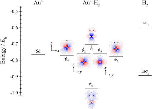
Figure 2. Molecular orbital diagram for Au⁺–CO. See text for details. The contours are the same for all molecular orbitals shown. For CO, the calculated orbital energies of the 2pσ and 2pπ orbitals in the absence of the coulombic field arising from the metal atom are indicated in grey, while the solid line indicates their energy in the presence of the field. The position of the gold nucleus is indicated by a black dot, and that of the carbon and oxygen nuclei by grey dots, with the carbon atom the one closest to the gold. Orbitals lie in the yz plane unless indicated by the presence of axes, where these axes are located on the Au⁺. In the latter cases, one or more of the CO atoms may not be visible.

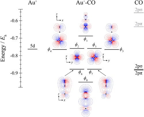
Figure 3. Molecular orbital diagram for Au⁺–N₂. See text for details. The contours are the same for all molecular orbitals shown. For N₂, the calculated orbital energies of the 2pσ_g and 2pπ_u orbitals in the absence of the coulombic field arising from the metal atom are indicated in grey, while the solid line indicates their energy in the presence of the field. The position of the gold nucleus is indicated by a black dot, and that of the nitrogen nuclei by grey dots. Orbitals lie in the yz plane unless indicated by the presence of axes, where these axes are located on the Au⁺. In the latter cases, one or more of the nitrogen atoms may not be visible.

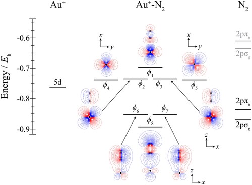
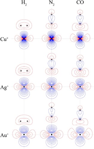
Figure 4. Contour plots for the HOMOs of the CM⁺–L complexes. See text for further comment and discussion. The position of the gold nucleus is indicated by a black dot, and that of the ligand nuclei by grey dots; in the case of CM⁺–CO, the carbon atom is closest to the gold. All orbitals lie in the yz plane.

For the Au⁺–H₂ complexes, the HOMO, ϕ₁, is formed from an antibonding combination between the outermost occupied Au⁺ $5d_{z^2}$ orbital and the 1sσ_g orbital on H₂; the corresponding bonding combination is ϕ₆. Both ϕ₂ and ϕ₃ are essentially non-bonding orbitals, while ϕ₄ and ϕ₅ involve a small interaction with the H₂ orbitals. In the case of ϕ₅, the main interaction is expected to be with the antibonding 1sσ_u orbital of hydrogen (not shown in Figure 1), which has the correct symmetry to interact with a 5d_yz orbital, and such an interaction is evident from the distortions in the contours of this orbital in Figure 1. Less obvious is the interaction that leads to ϕ₄ – this cannot involve σ orbitals, as these have the wrong symmetry, nor can it involve a π_u bonding orbital; in fact, it seems that ϕ₄ is formed from 5d_xz and the 2pπ_g antibonding orbital of H₂; this is surprising, given that this is expected to lie high in energy, but this seems to be the only symmetry-allowed possibility.

Considering the molecular orbital diagrams of both Au⁺–CO (Figure 2) and Au⁺–N₂ (Figure 3) together, these can be seen to be very similar, with even the expanded views of the HOMOs in Figure 4 indicating that the molecular orbitals are very similar for all CM⁺–CO and CM⁺–N₂ complexes. This is unsurprising, since these are valence isoelectronic species, and although there is a switch in the ordering of the outermost two occupied orbitals on the ligands, these are both still very close in energy and of different symmetry, so that they will interact with corresponding orbitals on CM⁺. As such, for the Au⁺–CO and Au⁺–N₂ complexes, we see that the orbitals ϕ₂–ϕ₅ are largely non-bonding, while ϕ₁ is the antibonding combination between the bonding σ orbital on the ligand and ϕ₈ is the corresponding bonding combination. It can also be seen that ϕ₆ and ϕ₇ arise from the bonding combination of each of the two bonding π orbitals on the ligand, and one of the 5d_yz and 5d_xz orbitals; these interactions are analogous to similar interactions in the Au⁺–H₂ complexes (Figure 1), but are much more evident in the present cases.

We remark that the effect on the ligand molecular orbitals when placed in the coulombic field of the cation is quite marked, with the orbitals lowering significantly in energy, meaning that the interactions with the CM⁺ atomic orbitals will be altered. As such, when considering interactions with metal cations, the energies of the ligand orbitals within the coulombic field need to be considered.

For the complexes involving the other two coinage metals, we expect that the diagrams will be similar, but the calculated atomic charges in Table 5 suggest that the corresponding molecular orbitals will have less covalency, particularly for the Ag⁺–containing complexes.

4. CM–L neutrals

4.1. Geometry, vibrational wavenumbers and interaction energies

The parameters for the optimised geometries of the neutral species are given in Tables 7–9, with the interaction energies in Table 10, and the calculated charges and spin densities in Table 11.

All methods yield linear geometries for each CM–H₂ complex, which are given in Table 7, and is in line with the linear geometry known for the H₃ molecule [57,66], whose existence had been proposed since 1911, but for which a spectrum was first measured serendipitously by Herzberg in 1979 [67]. Kuang et al. [37] also concluded a linear geometry for Cu–H₂ based upon DFT calculations employing the PW91 functional.

Table 7. Optimised geometries and vibrational wavenumbers of the linear CM–H₂ complexes (CM = Cu, Ag, Au)^a.

Method	Source^b	RCM–H / Å	rH–H / Å	σ / cm^–1	β / cm^–1	ωH–H / cm^–1
Cu–H2
B3LYP^c	Present work					(4413)
CAM-B3LYP	Present work	3.691	0.746 (0.745)	31	75	4400 (4407)
PW91	Present work	1.989	0.773 (0.749)	257	300	3849 (4330)
PW91	Ref. [37]	2.188	0.766
MP2	Present work	3.535	0.738 (0.737)	38	83	4505 (4518)
Ag–H2
B3LYP^c						(4413)
CAM-B3LYP	Present work	3.805	0.746 (0.745)	51	70	4401 (4407)
PW91	Present work	2.595	0.757 (0.749)	98	258	4171 (4330)
MP2	Present work	3.515	0.738 (0.737)	55	107	4501 (4518)
Au–H2
B3LYP	Present work	3.010	0.745 (0.743)	37	161	4367 (4413)
CAM-B3LYP	Present work	2.751	0.749 (0.745)	70	179	4336 (4407)
PW91	Present work	2.037	0.779 (0.749)	347	319	3741 (4330)
MP2	Present work	3.000	0.739 (0.737)	93	181	4478 (4518)

^a Where R_CM–H represents the shortest CM–H distance; r_H–H represents the H–H bond length in the complex, with the value in parentheses that calculated for uncomplexed H₂ at the same level of theory (only for the present work); σ represents the intermolecular stretch vibration; β the intermolecular bend vibration; and ω_H-H represents the H-H stretch vibration in the complex, with the value in parentheses that calculated for uncomplexed H₂ at the same level of theory (only for the present work).

^b The values calculated in the present work were obtained employing the ECP + aug-cc-pwCVTZ basis sets, as described in the main text. Otherwise, results are given for selected previous results, usually selecting the highest levels of theory; please consult the original reference for details of basis sets employed.

^c For Cu–H₂ and Ag–H₂, the optimisation using the B3LYP functional yielded a very long intermolecular bond length compared to the other methods, and the calculated parameters are not thought to be reliable, and hence are omitted. It is interesting that the same functional appeared to behave well for Au–H₂.

In the present work, the B3LYP functional gave rise to very long intermolecular separations for both Cu–H₂ and Ag–H₂, and it seems that the complex was simply dissociating; in contrast, the method gave a reasonable separation in the case of Au–H₂. It may also be seen that the vibrational wavenumbers vary considerably, with those for the PW91 functional being significantly higher, although in line with the significantly shorter intermolecular separations obtained using this method. Unfortunately, there are no experimental values to which to compare the intermolecular separations or vibrational wavenumbers.

For CM–CO and CM–N₂, it can be seen from the present and previous results, that there is significant variation in the geometries calculated, with some approaches yielding a linear geometry, while others produce a bent geometry. Notably, Møller-Plesset perturbation methods seem to favour a linear geometry for Cu–CO (see Table 8), but a bent geometry with DFT, QCISD, MCPF, CCSD and CCSD(T) approaches. From a computational chemistry point of view, and giving a higher weighting to the techniques that explicitly include higher levels of electron correlation, the consensus therefore is that Cu–CO does indeed have a bent geometry, and that earlier experimental conclusions that it was linear [6,7] appear to be incorrect, in line with results from infrared spectroscopic studies in inert gas matrices [8,9]. It is unknown why Møller-Plesset perturbation methods appear always to give rise to a linear geometry for Cu–CO.

Table 8. Optimised geometries and vibrational wavenumbers of the neutral CM–CO complexes (CM = Cu, Ag, Au)^a.

Method	Source^b	RCM-C / Å	rC–O / Å	θCMCO / °	σ / cm^–1	β / cm^–1	ωC–O / cm^–1
Cu–CO
B3LYP	Present work	1.918	1.140 (1.125)	141.9	359	234	2045 (2204)
B3LYP	Ref. [9]	1.969	1.144	138.6	328	222	2037
CAM-B3LYP	Present work	1.916	1.126 (1.121)	163.5	304	67	2178 (2248)
BP86	Ref. [9]	1.891	1.160	141.3	415	237	1958
PW91	Present work	1.852	1.155 (1.135)	143.7	439	250	1967 (2126)
MP2	Present work	1.771	1.143 (1.137)	180.0	431	69	2053 (2110)
MP2	Ref. [12]	1.791	1.144	180.0	372	104	2067
MP2	Ref. [15]	1.810	1.149	180	399	115	2073
MP4	Ref. [15]	1.690	1.189	180	662	474	1740
MCPF	Ref. [13]	1.964	1.132	153.1	300	162	2117
QCISD	Present work	1.907	1.131 (1.130)	168.5			(2180)
UCCSD(T)	Ref. [16]	1.880	1.142	154.2	317	133	2065
UCCSD(T)	Ref. [13]	1.910	1.140	152.5	323	159	2086
CCSD	Ref. [15]	2.002	1.135	156.9	239	119	2205
CCSD(T)	Ref. [15]	1.934	1.144	157.0	288	144	2108
Experiment	Ref. [9]						2009.8/2029.7^c
Experiment	Ref. [8]				323	208	2010^d
Ag–CO
B3LYP	Present work	2.315	1.135 (1.125)	130.2	229	131	2082 (2204)
B3LYP	Ref. [19]	2.636	1.133	125.4	164	45	2130
CAM-B3LYP	Present work	2.349	1.126 (1.121)	131.5	198	111	2159 (2248)
PW91	Present work	2.131	1.152 (1.135)	132.6	317	199	1971 (2126)
PW91	Ref. [19]	2.273	1.153	128.9	261	149	1985
MP2	Present work	3.373	1.138 (1.137)	118.1	19	160	2101 (2110)
MP2	Ref. [12]	diss.
UCCSD(T)	Ref. [16]	3.665	1.136	120.2	14^e	21^e	2137
Experiment	Ref. [19]						^c
Au–CO
B3LYP	Present work	2.035	1.139 (1.125)	142.0	362	230	2067 (2204)
B3LYP	Ref. [19]	2.093	1.148	125.4	330	211	2066
CAM-B3LYP	Present work	2.031	1.129 (1.121)	147.0	331	199	2147 (2248)
PW91	Present work	1.974	1.154 (1.135)	142.2	439	255	1976 (2126)
PW91	Ref. [19]	2.016	1.157	138.8	400	243	1973
MP2	Present work	1.954	1.148 (1.137)	150.0	388	184	1992 (2110)
MP2	Ref. [12]	2.159	1.137	180	223	131	2137
UCCSD(T)	Ref. [16]	2.018	1.143	148.0	293	146	2058
Experiment	Ref. [19]						2053^c

^a Where r_C–O represents the C–O bond length in the complex, with the value in parentheses that calculated for uncomplexed CO at the same level of theory (only for the present work); σ represents the intermolecular stretch vibration; β the intermolecular bend vibration; and ω_C–O represents the C–O stretch vibration in the complex, with the value in parentheses that calculated for uncomplexed CO at the same level of theory (only for the present work).

^b The values calculated in the present work were obtained employing the ECP + aug-cc-pwCVTZ basis sets, as described in the main text. Otherwise, results are given for selected previous results, usually selecting the highest levels of theory; please consult the original reference for details of basis sets employed.

^c Experimental fundamental values. For Cu–CO, the lower value was obtained by IR spectroscopy in an Ar matrix, while the higher value was in a Ne matrix. No absorption for Ag–CO was seen in Ref. [19]. The value for Au–CO was obtained in an Ar matrix.

^d Experimental fundamental value for the Cu–¹²C¹⁶O isotopologue using IR spectroscopy; values for other isotopologues were also reported in Ref. [8].

^e ω₀ value, as it was not possible to extract an ω_e value as there were too few bound levels.

For Ag–CO and Au–CO a linear geometry was assumed in EPR studies [17,18], but all present and previous calculated results in Tables 8 and 9 clearly suggest a bent geometry in both cases, even those using the MP2 method. We pointed out earlier that the B3LYP functional did not perform well for Cu–H₂ nor for Ag–H₂, although the results for Au–H₂ were in line with other methods. For the CM–CO complexes, the B3LYP functional also seemed to perform adequately; however, for Ag–N₂ and Au–N₂ the method was not satisfactory, giving rise to a long-range (and possibly dissociative) geometry; in contrast, for Cu–N₂, the method gave rise to a geometry similar to the other methods. Our general comment is that the B3LYP functional is not consistently reliable for such species.

Table 9. Optimised geometries and vibrational wavenumbers of the neutral CM–N₂ complexes (CM = Cu, Ag Au)^a.

Method	Source^b	RCM-N / Å	rN–N / Å	θCMNN / °	σ / cm^–1	β / cm^–1	ωN–N / cm^–1
Cu–N2
B3LYP	Present work	2.102	1.100 (1.091)	138.6	186	125	2295 (2445)
CAM-B3LYP	Present work	2.195	1.090 (1.086)	141.6	136	45	2422 (2497)
PW91	Present work	1.903	1.120 (1.101)	142.3	327	205	2132 (2352)
MP2	Present work	3.775	1.112 (1.112)	122.0	40	21	2189 (2194)
Ag–N2
B3LYP^c	Present work
CAM-B3LYP	Present work	4.809	1.086 (1.086)	127.5	11	6	2497 (2497)
PW91	Present work	3.675	1.101 (1.101)	126.8	53	23	2345 (2352)
MP2	Present work	3.768	1.112 (1.112)	121.8	45	24	2188 (2194)
UCCSD(T)	Ref. [32]	3.95	1.277^d	119.9
Au–N2
B3LYP^c	Present work
B3LYP	Ref. [33]	3.956	1.091	180^e			2352
CAM-B3LYP	Present work	3.945	1.086 (1.086)	128.0	29	14	2496 (2497)
PW91	Present work	2.214	1.113 (1.101)	136.1	207	144	2200 (2352)
PW91	Ref. [33]	3.463	1.102	180^e			2355
MP2	Present work	3.363	1.113 (1.112)	116.4	57	33	2184 (2194)

^a Where r_N–N represents the N–N bond length in the complex, with the value in parentheses that calculated for uncomplexed N₂ at the same level of theory (only for the present work); σ represents the intermolecular stretch vibration; β the intermolecular bend vibration; and ω_N–N represents the N–N stretch vibration in the complex, with the value in parentheses that calculated for uncomplexed N₂ at the same level of theory (only for the present work).

^b The values calculated in the present work were obtained employing the ECP + aug-cc-pwCVTZ basis sets, as described in the main text. Otherwise, results are given for selected previous results, usually selecting the highest levels of theory; please consult the original reference for details of basis sets employed.

^c For Ag–N₂ and Au–N₂, the optimisation using the B3LYP functional yielded a very long intermolecular bond length compared to the other methods, and the calculated parameters are not thought to be reliable, and so are omitted. The bending vibrational wavenumber was calculated to be imaginary, likely due to the flat potential and the use of numerical second derivatives; we did not pursue this further. It is interesting that the same functional appeared to behave well for Cu–N₂ (cf. the CM–H₂ complexes where again the B3LYP functional did not perform well, but apparently was fine for Au–H₂).

^d This was fixed at this value in Ref. [32].

^e In contrast to the our results, the geometry was calculated to be linear in Ref. [33] using the same functionals, but Pople-style basis sets.

With regard to vibrational wavenumbers, generally the B3LYP and PW91 functionals gave rise to what seem to be overly high bending vibrational wavenumbers (see below), but in fact the intermolecular vibrational wavenumbers are quite variable across the methods employed. A number of authors, from whom we highlight Bauschlicher [13], and Céron and Mendizabal [15], have noted how difficult it is to describe the Cu–CO complex using even quite sophisticated methods; the present work suggests this conclusion applies across most of the range for the neutral complexes considered in the present work, and this is particularly true of the intermolecular vibrational wavenumbers.

Returning to the CM–N₂ complexes, again bent geometries are calculated in the present work. Although there seems to be no experimental work that directly addresses the geometries of these complexes, there have been limited computational studies. Ag–N₂ has been studied at the UCCSD(T)/aug-cc-pVQZ level of theory [32], as part of a scattering study, employing the same small-core, relativistic ECP as used in the present work. Therein, a bent geometry was obtained, as with all of the methods employed herein; however, no vibrational wavenumbers were reported in that work. In contrast, Ding et al. [33] used DFT methods to conclude Au–N₂ was linear, while all methods employed herein, DFT or otherwise, conclude a bent geometry; we are unable to explain why that study yielded a linear structure.

Notwithstanding the general agreement that both the CM–CO and CM–N₂ complexes are bent, there is still quite a range of calculated intermolecular bond lengths and bond angles. Since the multireference character appears to be small, we favour the results of the UCCSD(T), MCPF and RQCISD results, which generally agree closely. Interestingly for DFT, some of the functionals also yield bent geometries and bond lengths and bond angles that are in line with those obtained using the other methods, but this is not generally true, and caution is merited in the use of DFT for such complexes.

In one of the Cu–CO IR matrix studies [8], the low-frequency intermolecular bending and stretching vibrational wavenumbers were measured, with the predominant isotopologue having reported respective values of 207.5 and 322.7 cm^–1. The latter value is in good agreement with values obtained using UCCSD(T) approaches, but the DFT methods give very variable values for the intermolecular stretch vibration. For the bending vibration, the calculated values are very erratic, with the UCCSD(T) methods suggesting much lower values than the experimental one. Although some DFT methods give rise to values that are at least consistent with the reported experimental value, we do not currently have confidence in these. As such, we suggest that it may be possible that the experimental value is not the fundamental, but an overtone of the bending mode, with the higher levels of theory suggesting that it may correspond to four quanta of the bending mode! To establish the experimental value more firmly, and hence to be able to ascertain which quantum chemical methods are performing the best, it will be necessary to record spectra in the range below 300 cm^–1 to establish whether other absorptions are seen, and whether a lower-wavenumber fundamental and overtones thereof can be assigned. Further, it is likely that the low-wavenumber intermolecular vibrations are highly anharmonic, and may mix for the bent geometries; as such, calculating high-quality potential energy surfaces, such as that for Ag–N₂ in Ref. [32], may be necessary, and the anharmonic vibrational wavenumbers and wavefunctions examined, such as was reported in Refs. [16,42].

We now move onto the interaction energies, which were calculated using single-point RCCSD(T) calculations using large basis sets and extrapolating to the basis set limit; this was done at a number of the optimised geometries obtained using a range of methods, including from other work, and the full results can be seen in the Supplementary Material. In particular, we highlight that the results obtained using three different extrapolations to the basis set limit are in very good agreement, for each geometry. Assuming that the RCCSD(T) method is the most reliable of the methods employed, then the best calculated interaction energy is expected to be the highest of the values obtained from the quadruple–ζ/quintuple–ζ extrapolation, and it is this value that is reported in Table 10. Many of the values are close, suggesting that the optimised geometries are close to the minimum on the basis-set-extrapolated RCCSD(T) potential surface, however, a number are significantly different, or even negative, such as that calculated for Cu–CO at the MP2-optimised geometry; indicating that the level of theory used for the optimisation method is not adequate for that species. In such cases, this indicates that the latter geometry is very different to that on the basis-set-extrapolated RCCSD(T) potential surface. As a consequence, it is deemed that the MP2 approach does not describe the Cu–CO complex well, in line with the linear geometry obtained with this method, in contrast to the bent geometries obtained with RQCISD and UCCSD(T) approaches. We are only aware of one experimental value, D₀ = 2100 ± 400 cm^–1, available for Cu–CO, and this can be seen to be in fair agreement with the present calculations, noting that the calculated value is a D_e value.

Perusal of the different interaction energies in the Supplementary Material shows that different methods perform very differently for the different complexes, emphasising the high demands of the CM–L complexes from the quantum chemistry. Interestingly, except for Cu–CO, the MP2 method does work well for the other complexes. On the other hand, results using DFT-optimised geometries are a little more erratic across the CM–L complexes, in agreement with comments made by Bauschlicher [13]. The final interaction energy for Cu–CO is higher than, but in reasonable agreement with values reported by Bauschlicher [13] using post-Hartree–Fock methods, who also showed that the value calculated with MP2 theory, which yielded a linear geometry, was almost three times the value calculated with other methods, and concurs with the negative value obtained using single-point RCCSD(T) calculations at the MP2-optimised geometry, in the present work.

Table 10 shows that Ag–CO is significantly more weakly bound than the other two complexes, as has been noted in previous work. A ΔZPVE value of ca. 25 cm^–1 then suggests a D₀ value of 110 cm^–1, which is very low, but would suggest that the complex could be produced in the gas-phase in a supersonic jet expansion, for example. The complex has been successfully observed in matrix isolation experiments [19] by Andrews’s group. The Au–CO complex is the most strongly bound, but the Cu–CO complex also has a significant interaction energy. Although there do not seem to be any experimental values to which to compare, the values are similar to those of Tielens et al. [20]; they are, however, significantly lower than those of Schwerdtfeger and Bowmaker. [12] In all cases for the CM–CO complexes, our values are close to, but higher than the values reported by Qawasmeh et al. [16] whose geometries were the ones that gave rise to our best values; as with the corresponding cation, the reason for this is the larger basis sets and the extrapolations used in the present work.

All of the CM–N₂ complexes are calculated to be very weakly bound, and will be even more so when accounting for ΔZPVE. For such weakly-bound species, the vibrations will be very anharmonic, and so could be significantly different from the calculated harmonic values. To our knowledge, except for some calculations where the geometry was fixed, and just the orbital energies were considered [30], there have been no experimental or quantum chemical calculations on the Cu–N₂ complex. In contrast, for Ag–N₂, a high-quality potential energy surface was calculated [32] at the UCSSD(T)/aug-cc-pVQZ level, using the same ECP28MDF pseudopotential as employed herein. Our greatest interaction energies were calculated at the minimum energy of that work, with our basis-set-extrapolated value being sizeably larger than that reported in Ref. [32]. Although the Au–N₂ complex is the most strongly bound of the three CM–N₂ complexes, the interaction energy is still remarkably low.

It is notable how much higher the interaction energies are for the CM–CO complexes compared to those of the CM–N₂ species, given the isoelectronic nature of the ligands – this will be discussed further hereinafter. The much weaker bonding of the CM–H₂ and CM–N₂ complexes is evident from the fact that the calculated H₂ and N₂ bond lengths do not change much upon complexation. On the other hand, there are significant lowerings of the CO vibrational wavenumber, and an increase in the CO bond length, indicating significant electron density shifts between CO and the incoming CM atom, as expected from the Dewar-Chatt-Duncanson mechanism [68,69].

Finally, the interaction energies for the CM–H₂ complexes are also very low – even lower than those of the CM–N₂ complexes. There are very few previous values to which to compare, but we highlight that the value of just over 900 cm^–1 by Kuang et al. [37] is over twenty times the calculated value here, and suggests the PW91 functional is not describing this complex well. This is consistent with the short intermolecular separations calculated using this method (both from Ref. [37] and the present work), compared to the CAM-B3LYP and MP2 calculations reported herein (see Table 7), and with the negative interaction energies calculated when the PW91 geometry was employed. Overall, we conclude that the PW91 functional overestimates the strength of the interactions in the CM–L complexes.

4.2. Charges and molecular orbital diagrams

The calculated atomic charges and spin densities for the CM–L complexes are given in Table 11 at two sets of optimised geometries. It may be seen that the three population methods generally give qualitatively the same picture, for both the CAM-B3LYP (PW91 for Ag–N₂) and MP2 geometries, with the unpaired electron being located almost exclusively on the metal atom, and very little charge transfer, although the charge distribution in the CO ligand varies significantly for the different population methods.

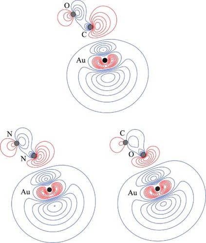
We now examine the molecular orbital plots of the Au–L complexes in Figures 5–7, where contour plots of the pertinent orbitals are shown; additionally, the forms of the CM–L HOMOs are directly comparable in Figure 8.

Figure 5. Molecular orbital diagram for Au–H₂. See text for details. The contours are the same for all molecular orbitals shown. The position of the gold nucleus is indicated by a black dot, and that of the hydrogen nuclei by grey dots. Orbitals lie in the yz plane unless indicated by the presence of axes, where these axes are located on the Au. In the latter cases, one or more of the hydrogen atoms may not be visible.

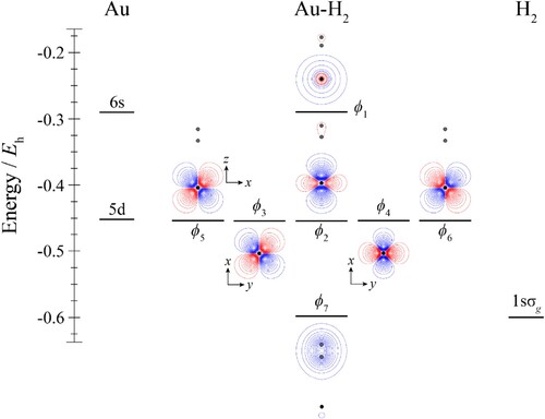
Figure 6. Molecular orbital diagram for Au–CO. See text for details. The contours are the same for all molecular orbitals shown. The position of the gold nucleus is indicated by a black dot, and that of the carbon and oxygen nuclei by grey dots, with the carbon atom the one closest to the gold. Orbitals lie in the yz plane unless indicated by the presence of axes, where these axes are located on the Au. In the latter cases, one or more of the CO atoms may not be visible.

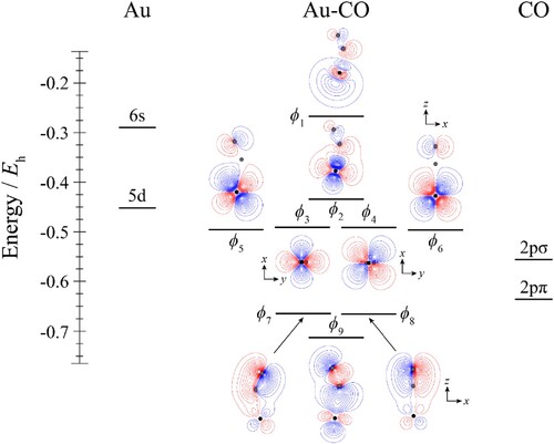
Figure 7. Molecular orbital diagram for Au–N₂. See text for details. The contours are the same for all molecular orbitals shown. The position of the gold nucleus is indicated by a black dot, and that of the nitrogen nuclei by grey dots. Orbitals lie in the yz plane unless indicated by the presence of axes, where these axes are located on the Au. In the latter cases, one or more of the nitrogen atoms may not be visible.

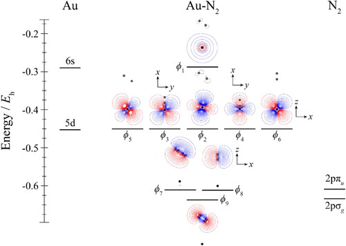
Figure 8. Contour plots for the HOMOs of the CM–L complexes. See text for further comment and discussion. The position of the gold nucleus is indicated by a black dot, and that of the ligand nuclei by grey dots; in the case of CM–CO, the carbon atom is closest to the gold. All orbitals lie in the yz plane.

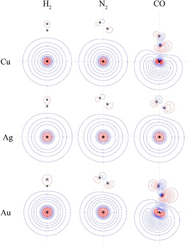
For Au–H₂, the molecular orbitals are as expected for the global, linear minimum, with the HOMO being merely a slight distortion of the outermost CM ns orbital, containing the unpaired electron. It can also be seen from Figure 5 that the Au 5d orbitals barely deviate from degeneracy, with only very little involvement of the H₂ orbitals; in addition, ϕ₇ is largely the 1sσ_g bonding orbital of H₂. This interaction is therefore largely physical in nature, in line with the low interaction energies and the high localisation of the unpaired electron on the Au atom. This picture also applies to the Cu–H₂ and Ag–H₂ complexes, based on the HOMO contour plots shown in Figure 8; indeed, the distortions of the 4s and 5s orbitals for Cu–H₂ and Ag–H₂, respectively, are even smaller in these cases. The physicality of the interaction is supported by the calculated atomic charges and spin densities given in Table 11, where there is very little charge transfer between the CM atom and the H₂ ligand; furthermore, the H(R_C) parameter is positive, but close to zero in all cases, indicating that there is essentially no covalent interaction.

We now consider the CM–CO and CM–N₂ complexes. The differences between the two ligands in coordination chemistry have been of interest for some time because of the very different interaction strengths that are seen. Mainly this has been looked at in terms of differences in the σ and π orbital energies and their make–up, but the dipole in CO has also been mentioned, and we would also point out the fact that CO has a higher quadrupole than N₂ – see Table 6. As discussed above, and as shown in Tables 8 and 9, all CM–CO and CM–N₂ complexes are deduced to have non-linear geometries. The contour plots of the HOMOs are given in Figure 8, and these clearly show that there is much more orbital sharing across CM and L for CM–CO complexes than for CM–N₂ complexes. Furthermore, the molecular orbital diagram for Au–CO in Figure 6 shows that there is a significant interaction involving the Au 6s, $5d_{z^2}$ and CO 2σ orbitals. This can be seen most clearly from the orbital contour plots, but also the pronounced deviation of the ϕ₂ orbital from the energy of the ϕ₃ and ϕ₄ orbitals, which are largely non-bonding 5d orbitals. It is interesting to note that these two orbitals lie significantly lower than the 5d atomic orbitals – this implies that there is some reduction in electron density on the Au atom, leading to an increased coulombic contribution to the atomic orbital energies, which is supported by the atomic charges and spin densities in Table 11.

There are small distortions of the d_xz and d_yz orbitals in forming the ϕ₅ and ϕ₆ molecular orbitals from an antibonding interaction between each 5d orbitals and one component of the 2pπ bonding orbital; this causes the section of the orbital close to Au to resemble a distorted 5d orbital, and also leads to a severe reduction in electron density around the C atom. Finally, we note that the HOMO plots for the three CM–CO complexes in Figure 8 look similar, but the largest interaction is occurring for Au–CO (as can be seen from the contours), followed by Cu–CO, with Ag–CO being the weakest. These observations are in line with the calculated interaction energies discussed above, and shown in Table 10.

Looking now at the MO diagram of Au–N₂ in Figure 7, it can be seen that there is now very little orbital mixing between the Au and N₂ orbitals, and this is confirmed by the forms of all of the molecular orbitals, and the close-to-degenerate nature of the ϕ₂–ϕ₆ molecular orbitals; nonetheless, these complexes are markedly bent, similar to the Au–CO complexes.

In the above, we rationalised the more-favourable interaction of the CM⁺ with the carbon end of CO as being due to the topography of the electron density, as discussed by Frenking et al. [65] where the higher local electron density on the carbon favours this approach. However, it is more difficult to explain the same favoured approach for the neutral CM atom, where consideration of electron repulsion would seem to disfavour this. To explore this, we examined the contours of the electron density when we artificially switched the locations of C and O for Au–CO. The contour plot for this is shown in Figure 9, where it can be compared to the actual arrangement. It can be seen that both plots are similar, but that the electron density is able to deform away from the incoming Au atom more easily in Au–CO than in Au–OC, which we attribute to the higher nuclear charge of O, and so the less polarisable electron density on that end of the molecule. Of course, we recognise that this is a simplistic explanation, and a number of effects are happening in concert, but this seems a reasonable ‘first-order’ explanation of the preferred interaction orientation with CO.

Figure 9. Contour plots of the HOMOs of the indicated CM–L complex, at the indicated geometry. The Au–L//Au–L′ notation employed indicates that the contours of Au–L are shown, calculated at the optimised geometry of Au–L′, with the latter calculated at the MP2 level of theory using the triple–ζ quality basis sets described in the main text. The position of the gold nucleus is indicated by a black dot, and that of the ligand nuclei by grey dots; in the case of Au–CO, the carbon atom is closest to the gold. All orbitals lie in the yz plane. See text for further discussion.

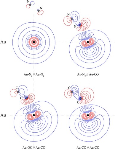
To address the question as to whether the difference in the strength of interaction originates from the difference between the CO and N₂ MOs, we have calculated the contours for the HOMO of Au–N₂ but now with the Au positioned at the same distance from the nearest N atom, as is the C atom from the Au atom in the Au–CO complex, and with the same bond angle. This diagram is also shown in Figure 9, and it may be seen that the HOMO contours are now very similar to those of Au–CO; as such, we conclude that the initial driver for the stronger CM–CO interactions is the larger physical interaction, arising from the CO dipole moment [70], and the larger quadrupole moment compared to that of nitrogen (see Table 6). This causes the CM and L moieties to get close enough together that distorting the electron density to reduce electron repulsion becomes an important consideration, which in turn allows the moieties to get even closer together, leading to a synergistic increase in the interaction energy. Owing to nuclear charge effects, we expect the electron density to be more polarisable on carbon than on nitrogen, and that on oxygen to be even less so – this expectation is met in the HOMO plots in Figure 9, and appears to be a contributing factor to the bonding direction of CO, and why Au–CO has a higher interaction energy than Au–N₂.

It can be seen from the Au–CO molecular orbital diagram (Figure 6) that there is some $\text{s}{\text{d}}_{z^2}$ hybridisation, which can be most clearly seen in the HOMO, ϕ₁, but also in ϕ₂ and ϕ₉. This hybridisation allows some of the 6s electron density to move off-axis, and away from the intermolecular region, reducing electron repulsion. There are also bonding overlaps between the 2pσ and 2pπ CO orbitals with the different Au 5d orbitals, as can be seen from ϕ_7–9. Part of the effect of this is to move charge density away from the Au atom, causing it to become δ+, and this adds an attractive coulomb term to the interaction. All of these effects add up to a significant binding energy, and are benefited from the energetic availability of the (n-1)d orbitals to relieve the repulsion that occurs between the 2pσ electrons on CO and the ns electron on CM. The 3d⁹4s² states of Cu lie at over 11,000 cm^–1, while the lowest Au 5d⁹6s² state lies at just over 9,000 cm^–1; on the other hand, the 4d⁹5s² states of Ag lie at over 30,000 cm^–1, explaining why the bonding in Ag–CO is much weaker than in both Cu–CO and Au–CO.

For the CM–N₂ complexes, we conclude that the balance between the attractive and repulsive terms of the interaction energy is more equal, and so the N₂ is located further away; we have shown that if the attractive terms were greater, then a very similar bonding picture would emerge as for the CM–CO complexes, with various synergistic effects occurring that both increase the influence of the attractive terms, while reducing that of the repulsive terms.

When comparing the CM–H₂ and CM–N₂ complexes, the binding energies are of a similar magnitude, but with those of the latter being greater – presumably because of the higher absolute magnitude of the quadrupole moment of N₂ compared to H₂, and the higher polarisability of N₂ compared to CO and H₂ – see Table 6 for quadrupole moment and polarisability values [71,72]. As noted earlier, the quadrupole moment of H₂ is positive, while those of N₂ (and CO) are negative, and this is the main driver for the observed geometries of the CM⁺–L complexes, although other factors are also significant. For the neutral complexes, again the positive quadrupole of H₂, arising from the formation of the 1sσ_g orbital, will favour the CM approaching from a linear orientation, to reduce electron repulsion. For L = N₂ and CO, this would favour the T-shaped orientation, but this simplistic argument is obscured by other factors, such as hybridisation and back bonding, which open up other means to reduce electron repulsion and also to provide a contribution from covalent terms. The net result of all of this is the observed bent geometries.

Some of these bonding effects can be seen in the changes in the ligand bond lengths and vibrational wavenumbers upon complexation. In the CM⁺–H₂ cations, the H–H bond length increases, and the vibrational wavenumber decreases, consistent with charge transfer from the metal to the ligand. On the other hand, the changes are rather small for the CM⁺–N₂ complexes, and a little variable for CM⁺–CO, but with a trend for an increase in the vibrational wavenumber in the latter case.

5. Further discussion and concluding remarks

Perhaps unsurprisingly, it is found that the more-strongly bound, closed-shell cations are easier to describe computationally than are the open-shell neutrals. Indeed, the latter are very problematic with results varying widely amongst the different methods reported in the literature and herein. The paucity of reliable experimental data makes judging the reliability of the different methods difficult, but the usual robustness of the (R)CCSD(T) approach would lead one to favour those results, which is supported by the calculations of Bauschlicher [13] when judged against the experimental interaction energy of Cu–CO. This contradicts the conclusions of Tremblay and Manceron [8], who commented that the B3LYP method appeared to give the best agreement with the intermolecular vibrational wavenumbers; we have suggested that one explanation for this could be that the experimental value may have been a higher overtone, which would then be consistent with the much lower values of the bending mode calculated using QCISD and UCCSD(T) approaches. Certainly for the CM–H₂ and CM–N₂ complexes, the B3LYP method performs poorly (see Tables 7 and 9), with only one complex apparently being described well, but a different one for each ligand! In addition, the other two functionals employed herein, and different ones employed in other publications, do not yet seem to yield a consistent conclusion. (Although the PW91 function did give optimised geometries in all cases, these had shorter intermolecular separations than higher-level methods.)

A more systematic study is required in evaluating the performance of DFT methods, including the role of dispersion corrections, which will be greatly aided by the provision of both first- and second-order analytic gradients for these. However, with the absence of reliable experimental data, either reliance must be based on convergence of calculated parameters with systematically improvement in the functionals (which is difficult with the wide variety of these), or it may be that agreement with high-level post-Hartree–Fock methods is judged to be a valid criterion. The Møller-Plesset perturbation theory approach appears to be robust for both cation and neutral systems, with the except of Cu–CO, where it performs poorly, giving an incorrect linear geometry. In all cases, it will be important to ensure that basis set variation is not the cause of the erratic nature of the calculated results, and we have been careful to be consistent on this point in the present work. Either way, conclusions will be more robust if a wider range of reliable experimental data were available, against which to calibrate the methods. (For the cations, the experimental data are mainly interaction energies; even then, the uncertainties are often significant.)

The different behaviour of H₂ and N₂ as homonuclear diatomic ligands is interesting, and highlights the role of molecular orbitals derived from the atomic 2p orbitals. The CM⁺–H₂ complexes are all T-Shaped, while the CM–H₂ neutral molecules are linear; in contrast, the CM⁺–N₂ complexes are linear, while the neutrals are bent, with the same types of geometries observed for the corresponding complexes with CO. For the CM⁺–N₂ and CM⁺–CO complexes, the main attraction term is electrostatic and driven by the charge-quadrupole interaction (see above), giving rise to the T-Shaped CM⁺–H₂ complexes (consistent with the triangular H₃⁺ geometry) [57] and the linear geometries of the other two sets of complexes. There is also a possible contribution from the ligand donating some electron density towards the CM⁺, and this is achieved via the sp hybrid orbitals for N₂ and CO, with the best orientation for this being linear. Any significant changes in electron density of the individual moieties, atomic or diatomic, will affect quantities like multipole moments and may need to be considered further.

For the neutrals, reduction of electronic repulsion plays a more significant role. Our results appear to show that there is a very subtle balance in the interactions, with the dipole moment and quadrupole moment of CO being the dominant factors in pulling the moieties together, while this is mainly the quadrupole in the cases of N₂ and H₂: the closer the approach, the larger the electrostatic attraction terms become (see Table 6 for quadrupole moment and dipole moment values), but also dispersion terms will become important. However, in each case repulsion will play a key role, but can be ameliorated if electron density can be reduced in the intermolecular region, by a combination of varying the orientation and hybridisation, both of which will modify the attractive terms; each of these could also lead to electron density movement, including partial charge transfer. By locating the N₂ artificially closer to Au, we find that both the N₂ and CO ligands behave similarly, with almost identical molecular orbitals (see Figure 9). As such, we conclude that the main difference between the CM–N₂ and CM–CO complexes is how close the ligand can get, and CO ‘wins’ owing to the greater, attractive multipolar terms. Interestingly, the CM–N₂ complexes are still bent at their equilibrium geometries, and it is likely that small CM → L donation occurs into the π* orbital of the ligand (hints of which are evident in the Au–N₂ molecular orbitals, such as ϕ₁ in Figure 7), which is favoured by a bent geometry; it is likely that there is a very subtle balance of effects in these weakly-bound species.

Hybridisation clearly plays a role in the CM–CO complexes. The forms of the HOMOs (Figure 8) and the other orbitals in the MO diagram of Au–CO (Figure 6) clearly show that the Au 6s and $5d_{z^2}$ orbitals hybridise, during the interaction with the 2pσ orbital of CO, for which one might anticipate a linear orientation. However, bending the complex allows an interaction between the 5d_yz and the in-plane component of the 2pπ CO orbital, together with interactions between the out-of-plane 2pπ and 5d_xz orbitals. It is a very fine balance of all of these orbital effects, combined with the electrostatics, that creates a very complicated set of interactions. As such, this may be one explanation as to the difficulty of describing these complexes using quantum chemistry methods, as each of these different contributions places different demands on the theoretical method and basis sets. Although we have mainly discussed the neutral Au–L complexes, similar arguments will apply to the complexes involving the other coinage metals, and we have discussed some of these in relation to the different effective sizes and also polarisabilities of the metal moiety. The starkest difference is that of the binding energy of Ag–CO which is significantly less than that of the other two CM–CO complexes, and although this is also the case for the corresponding cations, the difference is nowhere near as marked. This emphasises the synergistic nature of the different contributions to the bonding, such that once the moieties have an impetus to be closer, a number of other factors give rise to a large increase the interaction energy, while if this impetus is not present, then a weak interaction results; nonetheless, the relatively-low binding energy of Ag–CO remains notable.

Comparing the interaction energies with those of the CM⁽⁺⁾–RG (RG = He–Rn) complexes, summarised in Table 12, compiled from values reported by our group [73,74], we see no such sudden drop in the interaction energies of the Ag–RG complexes, and the CM–RG interaction energies increase monotonically for CM = Cu–Au. There is, however, a dip for the corresponding cations, again emphasising that the interactions are a balance of a number of effects. It can be seen that the interaction energies of Cu–CO and Au–CO are larger than those of the corresponding CM–RG complexes, and although this is also true of the cations, the difference is not so large.

Table 10. Interaction energies (cm^–1) for the CM–L complexes^a.

	CO	N2	H2
Cu	2740 [2100 ±400] [11]	66	44
Ag	140	114	50
Au	3282	130	97

^a Values reported are our best D_e values that have been calculated using RCCSD(T) single-point calculations at a geometry calculated at a lower level of theory, and have been corrected for basis set superposition error – see text for more details. The only available experimental (D₀) value is given in square brackets. Comments on other calculated values can be found in the text.

Table 11. Calculated atomic charges (Q), spin densities (ρ), and H(R_C) parameters for CM–L using different methods^a.

			CAM-B3LYP^b,c,d			MP2^b,c,e
CM	Quantity	Method	CM–N1N2	CM–C1O2	CM–H1H2	CM–N1N2	CM–C1O2	CM–H1H2
Cu	QCu	Mulliken	−0.010	−0.093	−0.004	−0.010	−0.082	−0.009
		NPA	−0.002	−0.068	0.000	−0.005	−0.077	0.001
		AIM	0.025	0.015	0.005	0.010	−0.003	0.006
	Q1	Mulliken	0.044	0.353	0.044	0.010	0.439	0.024
		NPA	−0.071	0.583	−0.002	−0.002	0.591	−0.003
		AIM	−0.094	1.280	−0.004	−0.011	1.283	−0.005
	Q2	Mulliken	−0.034	−0.260	−0.041	0.000	−0.357	−0.015
		NPA	0.073	−0.515	0.001	0.007	−0.514	0.002
		AIM	0.069	−1.294	−0.001	0.001	−1.280	−0.002
	ρCu	Mulliken	0.975	0.987	1.000	1.006	1.034	1.004
		NPA	0.948	0.939	1.000	0.997	0.949	1.000
		AIM	0.941	0.998	1.000	0.985	0.997	1.001
	ρ1	Mulliken	−0.002	−0.001	−0.002	−0.007	−0.037	−0.005
		NPA	0.036	0.055	0.000	−0.001	0.049	0.000
		AIM	0.043	0.002	0.000	0.010	0.003	0.000
	ρ2	Mulliken	0.027	0.014	0.002	0.001	0.004	0.001
		NPA	0.016	0.006	0.000	0.004	0.002	0.000
		AIM	0.016	0.000	0.000	0.004	0.000	0.000
	H(RC)		−0.009	−0.034	0.000	0.000	−0.068	0.000
Ag	QAg	Mulliken	−0.021	0.008	−0.005	−0.018	−0.013	−0.010
		NPA	−0.005	0.016	0.001	−0.005	−0.001	0.003
		AIM	0.014	0.018	0.006	0.013	0.020	0.008
	Q1	Mulliken	0.015	0.287	0.020	0.012	0.397	−0.026
		NPA	−0.004	0.423	−0.003	−0.003	0.479	−0.005
		AIM	−0.016	1.169	−0.005	−0.015	1.177	−0.008
	Q2	Mulliken	0.006	−0.295	−0.015	0.006	−0.383	0.035
		NPA	0.009	−0.439	0.002	0.008	−0.478	0.003
		AIM	0.003	−1.187	0.000	0.002	−1.198	0.000
	ρAg	Mulliken	1.016	0.910	1.001	1.013	1.016	1.004
		NPA	0.995	0.893	0.998	0.996	0.981	0.996
		AIM	0.979	0.890	0.991	0.981	0.962	0.987
	ρ1	Mulliken	−0.014	0.063	−0.003	−0.012	−0.018	−0.005
		NPA	0.001	0.076	0.000	−0.002	0.010	0.001
		AIM	0.016	0.073	0.007	0.013	0.027	0.010
	ρ2	Mulliken	−0.002	0.027	0.003	−0.002	0.002	0.001
		NPA	0.004	0.031	0.002	0.006	0.009	0.003
		AIM	0.005	0.036	0.002	0.007	0.012	0.003
	H(RC)		0.000	−0.011	0.000	0.000	0.001	0.000
Au	QAu	Mulliken	−0.001	−0.028	−0.007	−0.008	−0.097	−0.009
		NPA	−0.006	−0.042	0.015	−0.006	−0.026	0.008
		AIM	0.005	−0.051	0.012	0.008	−0.044	0.009
	Q1	Mulliken	0.034	0.348	−0.037	0.009	0.530	−0.080
		NPA	0.000	0.445	−0.018	−0.006	0.433	−0.009
		AIM	−0.006	1.214	−0.001	−0.012	1.190	−0.002
	Q2	Mulliken	−0.032	−0.321	0.044	−0.001	−0.433	0.089
		NPA	0.006	−0.403	0.003	0.012	−0.407	0.001
		AIM	0.001	−1.163	−0.011	0.004	−1.146	−0.007
	ρAu	Mulliken	1.001	0.827	0.993	1.007	0.943	1.004
		NPA	0.999	0.791	1.001	0.994	0.777	1.000
		AIM	0.992	0.815	1.001	0.982	0.807	1.001
	ρ1	Mulliken	−0.001	0.145	−0.008	−0.008	0.046	−0.006
		NPA	0.001	0.193	0.000	0.045	0.207	0.000
		AIM	0.007	0.153	−0.001	0.052	0.161	−0.001
	ρ2	Mulliken	0.000	0.027	0.016	0.001	0.011	0.002
		NPA	0.001	0.017	−0.001	−0.039	0.016	0.000
		AIM	0.001	0.032	0.000	−0.034	0.032	0.000
	H(RC)		0.000	−0.059	0.001	0.001	−0.082	0.001

^a See text for details; charges calculated using the geometry obtained using CAM-B3LYP/aug-cc-pwCVTZ or MP2/aug-cc-pwCVTZ (see Tables 7–9).

^b For clarity, the ligand atom closest to CM is always labelled 1.

^c For Cu–CO, the NPA and AIM charges were calculated using the ROHF density, owing to technical issues with the NPA program with the UQCISD density; in all other cases the UQCISD density was employed.

^d For Ag–N₂, the PW91 geometry was employed, as the CAM-B3LYP geometry is not thought to be reliable.

^e For Cu–CO, the MP2 geometry is not thought to be reliable, but the charges are included here for completeness.

Table 12. Calculated interaction energies (cm^–1) for the CM⁽⁺⁾–RG complexes^a.

	Cu		Ag		Au
RG	Neutral	Cation	Neutral	Cation	Neutral	Cation
He	6	790	8	396	15	385
Ne	22	842	28	575	47	565
Ar	91	4212	114	2607	185	3745
Kr	144	5890	169	3878	300	6155
Xe	224	8301	2534	5864	590	10063
Rn	334	9264	356	6822	819	11754

^a Values taken from Refs. [73,74].

The interaction energies reported in the present work are likely the most reliable to date, but geometries and vibrational wavenumbers from the present, and previous work, likely will require calculation of higher-level PESs, and extraction of anharmonic vibrational wavenumbers from these. Although some effort has been made to understand the interactions in these species, particularly of the carbonyls [27–29], with various decomposition schemes.

Finally, we feel the use of DFT methods for the neutral complexes should be treated with a large degree of caution, as also concluded by others [13,28]. It is likely that high-level post-HF methods, such as (R/U)CCSD(T), are required and, in some circumstances multireference character may need to be considered, particularly if the d orbitals are more intimately involved. Large basis sets, with polarisation and diffuse functions, are likely required for any hope of gaining quantitative results. For the cations, however, most methods seem to perform adequately, although obviously higher-level methods and similarly large basis sets will give rise to the most reliable results. In many catalytic environments, the metal is likely to carry a partial charge, and as such caution will certainly be merited in the use of DFT methods.

Acknowledgements

We acknowledge access to the University of Nottingham High Performance Computing Facility.

Disclosure statement

No potential conflict of interest was reported by the author(s).

Data availability statement

The data that support the findings of this study are available from the corresponding author upon reasonable request.

Additional information

Funding

We thank the University of Nottingham for a studentship to A.R.D. HA is grateful for a studentship awarded under the Engineering and Physical Sciences Research Council (EPSRC) CDT in Sustainable Chemistry (EP/S022236/1) and also for support under the EPSRC programme grant ‘MASI’ (EP/V000055/1).

References

- G. Pacchioni, Phys. Chem. Chem. Phys. 15, 1737–1757 (2013). doi:10.1039/C2CP43731G.
- C. Rivera-Cárcamo and P. Serp, ChemCatChem. 10, 5058–5091 (2018). doi:10.1002/cctc.201801174.
- G.S. Parkinson, Catal. Lett. 149 (5), 1137–1146 (2019). doi:10.1007/s10562-019-02709-7.
- C. Gerber and P. Serp, Chem. Rev. 120, 1250–1349 (2020). doi:10.1021/acs.chemrev.9b00209.
- M. Zhou, L. Andrews and C.W. Bauschlicher Jr., Chem. Rev. 101, 1931–1961 (2001). doi:10.1021/cr990102b.
- P.H. Kasai and P.M. Jones, J. Am. Chem. Soc. 107, 813–818 (1985). doi:10.1021/ja00290a013.
- J.H.B. Chenier, C.A. Hampson, J.A. Howard and B. Mile, J. Phys. Chem. 93, 114–117 (1989). doi:10.1021/j100338a026.
- B. Tremblay and L. Manceron, Chem. Phys. 242, 235–240 (1999). doi:10.1016/S0301-0104(99)00027-0.
- M. Zhou and L. Andrews, J. Chem. Phys. 111, 4548–4557 (1999). doi:10.1063/1.479216.
- L. Jiang and Q. Xu, J. Phys. Chem. A. 111, 2690–2696 (2007). doi:10.1021/jp067050w.
- M.A. Blitz, S.A. Mitchell and P.A. Hackett, J. Phys. Chem. 95, 8719–8726 (1991). doi:10.1021/j100175a055.
- P. Schwerdtfeger and G.A. Bowmaker, J. Chem. Phys. 100, 4487–4497 (1994). doi:10.1063/1.466280.
- C.W. Bauschlicher Jr., J. Chem. Phys. 100, 1215–1218 (1994); Erratum, J. Chem. Phys. 101, 1215 (1994). doi:10.1063/1.46665. Erratum: doi:10.1063/1.468521.
- V. Barone, Chem. Phys. Lett. 233, 129–133 (1995). doi:10.1016/0009-2614(94)01404-J.
- M.L. Cerón and F. Mendizabal, J. Chilean Chem. Soc. 48, 81–87 (2003). doi:10.4067/S0717-97072003000400013.
- Y. Qawasmeh, K. Töpfer, T. Serwatka, J.C. Tremblay, and B. Paulus, Molec. Phys. 119, e1892224 (2021). doi:10.1080/00268976.2021.1892224.
- P.H. Kasai and P.M. Jones, J. Phys. Chem. 89, 1147–1151 (1985). doi:10.1021/j100253a019.
- P.H. Kasai and P.M. Jones, J. Am. Chem. Soc. 107, 6385–6389 (1985). doi:10.1021/ja00308a038.
- B. Liang and L. Andrews, J. Phys. Chem. A. 104, 9156–9164 (2000). doi:10.1021/jp001833e.
- F. Tielens, L. Gracia, V. Polo and J. Andrés, J. Phys. Chem. A. 111, 13255–13263 (2007). doi:10.1021/jp076089d.
- X.-J. Kuang, X.-Q. Wang and G.-B. Liu, Catal. Lett. 137, 247–254 (2010). doi:10.1007/s10562-010-0357-5.
- T.K. Dargel, R.H. Hertwig, W. Koch and H. Horn, J. Chem. Phys. 108, 3876–3885 (1998). doi:10.1063/1.475791.
- D. Schröder, J. Hrušák, R.H. Hertwig, W. Koch, P. Schwerdtfeger and H. Schwartz, Organometallics. 14, 312–316 (1995). doi:10.1021/om00001a045.
- M. Neumaier, F. Weigend, O. Hampe and M.M. Kappes, J. Chem. Phys. 122, 104702 (2005). doi:10.1063/1.1854619.
- H. Schwarz, Angew. Chem. Int. Ed. Eng. 42, 4442–4454 (2003). doi:10.1002/anie.200300572.
- F. Meyer, Y.-M. Chen and P.B. Armentrout, J. Am. Chem. Soc. 117, 4071–4081 (1995). doi:10.1021/ja00119a023.
- A.J. Lupinetti, S. Fau, G. Frenking and S.H. Strauss, J. Phys. Chem. A. 101, 9551–9559 (1997). doi:10.1021/jp972657l.
- A.J. Lupinetti, V. Jonas, W. Thiel, S.H. Strauss and G. Frenking, Chem. Eur. J. 5, 2573–2583 (1999). doi:10.1002/(SICI)1521-3765(19990903)5:9<2573::AID-CHEM2573>3.0.CO;2-J.
- E. Rossomme, C.N. Liniger, A.T. Bell, T. Head-Gordon and M. Head-Gordon, Phys. Chem. Chem. Phys. 22, 781–798 (2020). doi:10.1039/C9CP04643G.
- S.G. Gagarin, Y.A. Teterin and I.G. Fal’kov, J. Struct. Chem. 25, 5–9 (1984). doi:10.1007/BF00808542.
- M.T. Rodgers, B. Walker and P.B. Armentrout, Int. J. Mass Spectrom. 182/183, 99–120 (1999). doi:10.1016/S1387-3806(98)14228-8.
- J. Loreau, P. Zhang and A. Dalgarno, J. Chem. Phys. 136, 164305 (2012). doi:10.1063/1.3703518.
- X. Ding, J. Yang, J.G. Hou and Q. Zhu, J. Molec. Struct. Theochem. 755, 9–17 (2005). doi:10.1016/j.theochem.2005.05.024.
- F.-X. Li, K. Gorham and P.B. Armentrout, J. Phys. Chem A. 114, 11043–11052 (2010). doi:10.1021/jp100566t.
- V. Dryza, B.L.J. Poad and E.J. Bieske, Phys. Chem. Chem. Phys. 14, 14954–14954 (2012). doi:10.1039/C2CP41622K.
- V. Dryza and E.J. Bieske, Int. Rev. Phys. Chem. 32, 559–587 (2013). doi:10.1080/0144235X.2013.810489.
- X.-J. Kuang, X.-Q. Wang and G.-B. Liu, J. Chem. Sci. 123, 743–754 (2011). doi:10.1007/s12039-011-0130-3.
- J.L. Elkind and P.B. Armentrout, J. Phys. Chem. 90, 6576–6586 (1986). doi:10.1021/j100282a031.
- P. Maître and C.W. Bauschlicher Jr., J. Phys. Chem. 97, 11912–11920 (1993). doi:10.1021/j100148a012.
- P.R. Kemper, P. Weis, M.T. Bowers and P. Maître, J. Am. Chem. Soc. 120, 13494–13502 (1998). doi:10.1021/ja9822658.
- S. Pakhra, T. Debnath, K. Sen and A.K. Das, J. Chem. Sci. 128, 621–631 (2016). doi:10.1007/s12039-016-1054-8.
- D.G. Artiukhin, E.J. Bieske and A.A. Buchachenko, J. Phys. Chem. A. 120, 5006–5015 (2016). doi:10.1021/acs.jpca.5b12700.
- V. Dryza and E.J. Bieske, J. Phys. Chem. Lett. 2, 719–724 (2011). doi:10.1021/jz200173m.
- K. Sen, S. Pakhira, C. Sahu and A.K. Das, Molec. Phys. 112, 182–188 (2014). doi:10.1080/00268976.2013.805849.
- H.W. Ghebriel and A. Kshirsagar, J. Chem. Phys. 126, 244705 (2007). doi:10.1063/1.2743420.
- F. Li, C.S. Hinton, M. Citir, F. Liu and P.B. Armentrout, J. Chem. Phys. 134, 024310 (2011). doi:10.1063/1.3514899.
- H.-J. Werner, P.J. Knowles, G. Knizia, F.R. Manby, M. Schütz, P. Celani, T. Korona, R. Lindh, A. Mitrushenkov, G. Rauhut, K.R. Shamasundar, T.B. Adler, R.D. Amos, A. Bernhardsson, A. Berning, D.L. Cooper, M.J.O. Deegan, A.J. Dobbyn, F. Eckert, E. Goll, C. Hampel, A. Hesselmann, G. Hetzer, T. Hrenar, G. Jansen, C. Köppl, Y. Liu, A.W. Lloyd, R.A. Mata, A.J. May, S.J. McNicholas, W. Meyer, M.E. Mura, A. Nicklaß, D.P. O'Neill, P. Palmieri, D. Peng, K. Pflüger, R. Pitzer, M. Reiher, T. Shiozaki, H. Stoll, A.J. Stone, R. Tarroni, T. Thorsteinsson and M. Wang. MOLPRO is a package of ab initio programs.
- H.J. Werner, P.J. Knowles, G. Knizia, F.R. Manby and M. Schütz, WIRES Comput. Mol. Sci. 2, 242 (2012).
- M.J. Frisch, G.W. Trucks, H.B. Schlegel, G.E. Scuseria, M.A. Robb, J.R. Cheeseman, G. Scalmani, V. Barone, G.A. Petersson, H. Nakatsuji, X. Li, M. Caricato, A.V. Marenich, J. Bloino, B.G. Janesko, R. Gomperts, B. Mennucci, H.P. Hratchian, J.V. Ortiz, A.F. Izmaylov, J.L. Sonnenberg, D. Williams-Young, F. Ding, F. Lipparini, F. Egidi, J. Goings, B. Peng, A. Petrone, T. Henderson, D. Ranasinghe, V.G. Zakrzewski, J. Gao, N. Rega, G. Zheng, W. Liang, M. Hada, M. Ehara, K. Toyota, R. Fukuda, J. Hasegawa, M. Ishida, T. Nakajima, Y. Honda, O. Kitao, H. Nakai, T. Vreven, K. Throssell, J.A. Montgomery Jr., J.E. Peralta, F. Ogliaro, M.J. Bearpark, J.J. Heyd, E.N. Brothers, K.N. Kudin, V.N. Staroverov, T.A. Keith, R. Kobayashi, J. Normand, K. Raghavachari, A.P. Rendell, J.C. Burant, S.S. Iyengar, J. Tomasi, M. Cossi, J.M. Millam, M. Klene, C. Adamo, R. Cammi, J.W. Ochterski, R.L. Martin, K. Morokuma, O. Farkas, J. Foresman and D.J. Fox, Gaussian 16: Revision A.03 (Gaussian, Inc., Wallingford, CT, 2016).
- A. Halkier, T. Helgaker, P. Jørgensen, W. Klopper, H. Koch, J. Olsen and A.K. Wilson, Chem. Phys. Lett. 286, 243–252 (1998). doi:10.1016/S0009-2614(98)00111-0.
- A. Halkier, T. Helgaker, P. Jørgensen, W. Klopper, H. Koch and J. Olsen, Chem. Phys. Lett. 302, 437–446 (1999). doi:10.1016/S0009-2614(99)00179-7.
- T.J. Lee and P.R. Taylor, Int. J. Quant. Chem. S23, 199–207 (1989). doi:10.1002/qua.560360824.
- J. Wang, S. Manivasagam and A.K. Wilson, J. Chem. Theory Comput. 11, 5865–5872 (2015). doi:10.1021/acs.jctc.5b00861.
- E.D. Glendening, A.E. Reed, J.E. Carpenter and F. Weinhold. NBO Version 3.1.
- T.A. Keith and T.K. Gristmill, Software (AIMAll, Overland Park, KS, 2011). see aim.tkgristmill.com.
- G. Schaftenaar and J.H. Noordik. Molden: A Pre- and Post-Processing Program for Molecular and Electronic Structures, J. Comput. Aided Mol. Des. 14, 123–134 (2000). doi:10.1023/A:1008193805436.
- H. Kragh, Astrophy. Geophys. 51, 6.25–6.27 (2010). doi:10.1111/j.1468-4004.2010.51625.x.
- T.G. Wright and W.H. Breckenridge, J. Phys. Chem. A. 114, 3182–3189 (2010). doi:10.1021/jp9091927.
- D. Bellert and W.H. Breckenridge, Chem. Rev. 102, 1595–1622 (2002). doi:10.1021/cr980090e.
- P. Pyykkö, Chem. Soc. Rev. 37, 1967–1997 (2008). doi:10.1039/B708613J.
- T.G. Wright, W.H. Breckenridge and V.L. Ayles, J. Phys. Chem. A. 112, 4209–4214 (2008). doi:10.1021/jp711886a.
- D.B. Lawson and J.F. Harrison, J. Phys. Chem. A. 101, 4781–4792 (1997). doi:10.1021/jp9703420.
- J.M. Junqera-Hernández, J. Sánchez-Marín and D. Maynau, Chem. Phys. Lett. 359, 343–348 (2002). doi:10.1016/S0009-2614(02)00722-4.
- D. Cremer and E. Kraka, Angew. Chem. Int. Ed. Engl. 23, 627–628 (1984). doi:10.1002/anie.198406271.
- G. Frenking, C. Loschen, A. Krapp, S. Fau and S.H. Strauss, J. Comp. Chem. 28, 117–126 (2007). doi:10.1002/jcc.20477.
- D. Stevenson and J. Hirschfelder, J. Chem. Phys. 5, 933–940 (1937). doi:10.1063/1.1749966.
- G. Herzberg, J. Chem. Phys. 70, 4806–4807 (1979). doi:10.1063/1.437272.
- M.J.S. Dewar, Bull. Soc. Chim. France. C18, 71–79 (1951).
- J. Chatt and L.A. Duncanson, J. Chem. Soc, 2939–2947 (1953). doi:10.1039/JR9530002939.
- J.S. Muenter, J. Molec. Spectrosc. 55, 490–491 (1975). doi:10.1016/0022-2852(75)90287-8.
- O. Christiansen, C. Hättig and J. Gauss, J. Chem. Phys. 109, 4745–4757 (1998). doi:10.1063/1.477086.
- R.L. Wilkens and H.S. Taylor, J. Chem. Phys. 48, 4934–4937 (1968). doi:10.1063/1.1668159.
- A. Yousef, S. Shrestha, L.A. Viehland, E.P.F. Lee, B.R. Gray, V.L. Ayles, T.G. Wright and W.H. Breckenridge, J. Chem. Phys. 127, 154309 (2007). doi:10.1063/1.2774977.
- A.M. Gardner, R.J. Plowright, M.J. Watkins, T.G. Wright and W.H. Breckenridge, J. Chem. Phys. 132, 184301 (2010). doi:10.1063/1.3386239.