On the origin of bonding in metals: lithium as a case study

Abstract

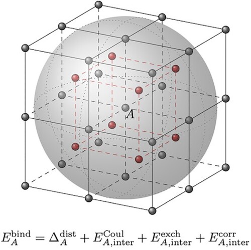
The bonding in metals is analysed within the framework of the PATMOS (Perturbed AToms in MOlecules and Solids) model. The electronic binding energy per atom is written as a sum of a distortion energy of the atoms and the partitioned interaction energy comprising Coulombic, exchange and correlation terms. The adopted physical model of the infinite system, is spherical embedding of the atoms of the reference unit cell. Correlation energies are calculated by second-order Møller-Plesset and second-order Epstein-Nesbet perturbation theory. The binding energy of lithium solid is calculated for 16 nearest neighbour distances from 4.0 to 10.0 Bohr. Electron correlation is of paramount importance for the binding energy. The calculated cohesive energy is $(0.0571\pm 0.004)$ Hartree comparing with experimental value 0.0599 Hartree. The bonding picture is characterised by slightly expanded atomic orbitals.

GRAPHICAL ABSTRACT

Keywords:

• PATMOS model
• energy partitioning
• electron correlation
• metals
• bonding

1. Introduction

Metallic bonding is apparently very different from bonding in polyatomic molecules. The latter is localised and directional. For a huge class of molecules, it can be described by localised electron-pair bonds [1]. According to Ruedenberg and coworkers [2], it is the quantum mechanical interference of wave functions of fragments that leads to the kinetic energy decrease in the system – which becomes the driving force behind chemical bonding. Most of studies have agreed upon the Ruedenberg's framework though fine details may diverge for different theoretical methods [3]. This picture of electron-pair bonding is not easily transferred to a metal. For an alkali metal with a bcc-structure, there are eight nearest-neighbour atoms for a particular atom, but only one valence electron for each atom. Hence, a system of electron-pair bonds for the metal is indeed difficult to imagine. To cope with this enigma it is customary to suppose that a metal is characterised by a delocalised ‘sea’ of electrons and that this ‘sea’ of negative charge holds the atoms together. The corresponding mathematical model is Hartree-Fock theory with delocalised orbitals, i.e. canonical Hartree-Fock orbitals. However, within the one-determinant approximation, the wave function is invariant with respect to a unitary transformation of the orbitals. A delocalised picture can be transferred to a localised picture. Accordingly, the original problem of explaining bonding is as puzzling as before. The scientific community has then more or less disregarded this particular problem and instead focussed on what can be obtained by molecular orbital theory with delocalised orbitals. An extensive body of scientific work demonstrates the success of this approach.

One of the difficulties of explaining bonding in metals can be traced back to a simplistic interpretation of the electron-pair bond concept. It is often interpreted as if electrons in complexes prefer to stick together in pairs. However, electrons repel each other, and left to themselves they separate. As for the ground state of a system, electrons try to come as close as possible to the nuclei in accordance with the Pauli exclusion principle. For localised orbitals we might interprete the Pauli principle as stating that two electrons with different spins can occupy the same part of the physical space. In order to obtain the lowest possible total energy for the system, the electrons arrange themselves in such a way that they are close to a nuclues or a pair of nuclei. In electron-pair bonds an electron of an atom is shifted towards the nucleus of a neighbouring atom, and vice versa. This particular feature of the electron-pair bonding is demonstrated in a work by Røeggen and Gao [4]. By moving away from the paring concept but keeping its physical content of the bonding, i.e. shifting of electrons in direction of neightboring atoms, bonding in metals might be more easily understood.

Another key to understand bonding in metals is related to the electron density. The density in metals is not very different from the sum of the atomic densities of isolated atoms put in the positions of the nuclei of the metal. Hence, the atomic wave-functions are only modestly distorted in forming the metal. This fact has an important corollary. If one uses restricted Hartree-Fock in the study of metals, which implies doubly occupied orbitals, this feature of the metallic bond cannot be disclosed. Therefore, one should preferably use unrestricted Hartree-Fock as a basic approximation in describing metals since it is essential to have one spatial orbital for each valence electron.

The purpose of this work is twofold: first, to construct a workable computational model for ab initio studies of the electronic structure of atoms in three-dimensional lattices. Second, to understand the origin of bonding in metals. As for the first purpose, the PATMOS model [4,5] (Perturbed AToms in MOlecules and Solids) is a convenient starting point. PATMOS calculations on finite chains of metallic atoms strongly suggest that the electronic structure of the atoms of chains can be characterised by localised orbitals, i.e. distorted atoms. Hence, a physical model with spherical embedding around each atom of the reference unit cell, is appropriate. The spherical embedding guarantees correct symmetry. In this work we shall then demonstrate that ab initio calculations on metallic atoms in three-dimensional lattices are feasible.

The structure of the paper is as follows: The second section is devoted to a short description of the PATMOS model adapted to periodic systems. The third section focuses on a physical model of the solid using spherical embedding. The fourth section gives details on the computational aspects of the model. The fifth section is devoted to calculations on lithium atoms in a three-dimensional lattice. In the last section there is a discussion of the different sources of errors in this work.

2. The PATMOS model

To manage the electron correlation problem for large molecules, it is now well established that within the wave function framework local correlation models are required. The local models can be traced back to the fundamental works by Pulay and coworkers [6–9]. To avoid a large virtual orbital space, Pulay [6] proposed to remove the component of the localised occupied orbitals from the atomic basis. He denoted the modified basis projected atomic orbitals (PAO). In calculating the inter-atomic correlation energy one could then use the union of the PAO's for the atoms involved instead of the full virtual orbital space for the complex. Hence, a drastic reduction of the computation time could be achieved.

To date various local correlation models have been developed and applied for periodic systems, for instance, the local second-order Møller-Plesset theory (MP2) [10], divide-expand-consolidate MP2 [11] and cluster-in-molecule local correlation approach [12]. Another way of adapting local correlation methods to metals is to use the energy incremental scheme. The orbital energy incremental scheme was introduced by Nesbet [13], and refined by Stoll and coworkers [14–16], Røeggen [17,18], Bytautas and Ruedenberg [19], Voloshina and Paulus [20], and more recently by Paulus and Stoll [21]. The PATMOS model is formulated within the energy incremental scheme. In principle the correlation energy in PATMOS model can be calculated by any size extensive correlation model. The detailed description of the PATMOS model is given in our previous works [4,5]. In this work we sketch only the essential elements: the energy partitioning and the PATMOS basis set approach.

2.1. Energy partitioning

The total electronic energy of a complex can within the PATMOS framework, be written as (1) $\begin{array}{rl}{E}^{\mathrm{P}\mathrm{A}\mathrm{T}\mathrm{M}\mathrm{O}\mathrm{S}}& =\sum _{A=1}^{N_{\mathrm{a}\mathrm{t}\mathrm{o}\mathrm{m}\mathrm{s}}}(E_A^{\mathrm{U}\mathrm{H}\mathrm{F}}+E_A^{\mathrm{c}\mathrm{o}\mathrm{r}\mathrm{r}})\\ & +\sum _{A<B}^{N_{\mathrm{a}\mathrm{t}\mathrm{o}\mathrm{m}\mathrm{s}}}(E_{AB}^{\mathrm{C}\mathrm{o}\mathrm{u}\mathrm{l}}+E_{AB}^{\mathrm{e}\mathrm{x}\mathrm{c}\mathrm{h}}+E_{AB}^{\mathrm{c}\mathrm{o}\mathrm{r}\mathrm{r}})\\ & +\sum _{A<B<C}^{N_{\mathrm{a}\mathrm{t}\mathrm{o}\mathrm{m}\mathrm{s}}}{E}_{ABC}^{\mathrm{c}\mathrm{o}\mathrm{r}\mathrm{r}}+\cdots .\end{array}$(1) In Equation (1(1) $\begin{array}{rl}{E}^{\mathrm{P}\mathrm{A}\mathrm{T}\mathrm{M}\mathrm{O}\mathrm{S}}& =\sum _{A=1}^{N_{\mathrm{a}\mathrm{t}\mathrm{o}\mathrm{m}\mathrm{s}}}(E_A^{\mathrm{U}\mathrm{H}\mathrm{F}}+E_A^{\mathrm{c}\mathrm{o}\mathrm{r}\mathrm{r}})\\ & +\sum _{A<B}^{N_{\mathrm{a}\mathrm{t}\mathrm{o}\mathrm{m}\mathrm{s}}}(E_{AB}^{\mathrm{C}\mathrm{o}\mathrm{u}\mathrm{l}}+E_{AB}^{\mathrm{e}\mathrm{x}\mathrm{c}\mathrm{h}}+E_{AB}^{\mathrm{c}\mathrm{o}\mathrm{r}\mathrm{r}})\\ & +\sum _{A<B<C}^{N_{\mathrm{a}\mathrm{t}\mathrm{o}\mathrm{m}\mathrm{s}}}{E}_{ABC}^{\mathrm{c}\mathrm{o}\mathrm{r}\mathrm{r}}+\cdots .\end{array}$(1) ) $N_{\mathrm{a}\mathrm{t}\mathrm{o}\mathrm{m}\mathrm{s}}$ denotes the number of atoms in the physical model, $E_A^{\mathrm{U}\mathrm{H}\mathrm{F}}$ and $E_A^{\mathrm{c}\mathrm{o}\mathrm{r}\mathrm{r}}$ are respectively the unrestricted Hartree-Fock (UHF) energy and the correlation energy for atom A, $E_{AB}^{\mathrm{C}\mathrm{o}\mathrm{u}\mathrm{l}}$ and $E_{AB}^{\mathrm{e}\mathrm{x}\mathrm{c}\mathrm{h}}$ are respectively the Coulomb and exchange part of the interaction energy between the atoms A and B, and $E_{AB}^{\mathrm{c}\mathrm{o}\mathrm{r}\mathrm{r}}$ is the correlation energy between the same atoms. Effective atomic energies can be introduced (2) $E^{\mathrm{P}\mathrm{A}\mathrm{T}\mathrm{M}\mathrm{O}\mathrm{S}}=\sum _{A=1}^{N_{\mathrm{a}\mathrm{t}\mathrm{o}\mathrm{m}\mathrm{s}}}{E}_A^{\mathrm{e}\mathrm{f}\mathrm{f}},$(2) where (3) $\begin{array}{rl}{E}_A^{\mathrm{e}\mathrm{f}\mathrm{f}}& =E_A^{\mathrm{U}\mathrm{H}\mathrm{F}}+E_A^{\mathrm{c}\mathrm{o}\mathrm{r}\mathrm{r}}+\frac{1}{2}\sum _{B\ne A}^{N_{\mathrm{a}\mathrm{t}\mathrm{o}\mathrm{m}\mathrm{s}}}(E_{AB}^{\mathrm{C}\mathrm{o}\mathrm{u}\mathrm{l}}+E_{AB}^{\mathrm{e}\mathrm{x}\mathrm{c}\mathrm{h}}+E_{AB}^{\mathrm{c}\mathrm{o}\mathrm{r}\mathrm{r}})\\ & +\frac{1}{3}\{\sum _{\begin{array}{c}B,C\\ A<B<C\end{array}}^{N_{\mathrm{a}\mathrm{t}\mathrm{o}\mathrm{m}\mathrm{s}}}{E}_{ABC}^{\mathrm{c}\mathrm{o}\mathrm{r}\mathrm{r}}+\sum _{\begin{array}{c}B,C\\ B<A<C\end{array}}^{N_{\mathrm{a}\mathrm{t}\mathrm{o}\mathrm{m}\mathrm{s}}}{E}_{BAC}^{\mathrm{c}\mathrm{o}\mathrm{r}\mathrm{r}}+\sum _{\begin{array}{c}B,C\\ B<C<A\end{array}}^{N_{\mathrm{a}\mathrm{t}\mathrm{o}\mathrm{m}\mathrm{s}}}{E}_{BCA}^{\mathrm{c}\mathrm{o}\mathrm{r}\mathrm{r}}\}\\ & +\cdots .\end{array}$(3) An important term for a periodic system is the sum of effective atomic energies for the atoms in the reference cell: (4) $E_{\mathrm{u}\mathrm{c}}^{\mathrm{P}\mathrm{A}\mathrm{T}\mathrm{M}\mathrm{O}\mathrm{S}}=\sum _{A=1}^{N_{\mathrm{a}\mathrm{t}\mathrm{o}\mathrm{m}\mathrm{s}}^{\mathrm{u}\mathrm{c}}}{E}_A^{\mathrm{e}\mathrm{f}\mathrm{f}}.$(4) In Equation (4(4) $E_{\mathrm{u}\mathrm{c}}^{\mathrm{P}\mathrm{A}\mathrm{T}\mathrm{M}\mathrm{O}\mathrm{S}}=\sum _{A=1}^{N_{\mathrm{a}\mathrm{t}\mathrm{o}\mathrm{m}\mathrm{s}}^{\mathrm{u}\mathrm{c}}}{E}_A^{\mathrm{e}\mathrm{f}\mathrm{f}}.$(4) ) $N_{\mathrm{a}\mathrm{t}\mathrm{o}\mathrm{m}\mathrm{s}}^{\mathrm{u}\mathrm{c}}$ is the number of atoms in the unit cell. As we increase the number of atoms in the physical model, $E_{\mathrm{u}\mathrm{c}}^{\mathrm{P}\mathrm{A}\mathrm{T}\mathrm{M}\mathrm{O}\mathrm{S}}$ should converge to the corresponding value for the infinite system.

In this work we are interested in the binding energy per atom: (5) $E_A^{\mathrm{b}\mathrm{i}\mathrm{n}\mathrm{d}}=E_A^{\mathrm{e}\mathrm{f}\mathrm{f}}-E_A^{\mathrm{i}\mathrm{s}\mathrm{o}},$(5) where $E_A^{\mathrm{i}\mathrm{s}\mathrm{o}}$ is the energy of the isolated atom. Then it follows from Equation (3(3) $\begin{array}{rl}{E}_A^{\mathrm{e}\mathrm{f}\mathrm{f}}& =E_A^{\mathrm{U}\mathrm{H}\mathrm{F}}+E_A^{\mathrm{c}\mathrm{o}\mathrm{r}\mathrm{r}}+\frac{1}{2}\sum _{B\ne A}^{N_{\mathrm{a}\mathrm{t}\mathrm{o}\mathrm{m}\mathrm{s}}}(E_{AB}^{\mathrm{C}\mathrm{o}\mathrm{u}\mathrm{l}}+E_{AB}^{\mathrm{e}\mathrm{x}\mathrm{c}\mathrm{h}}+E_{AB}^{\mathrm{c}\mathrm{o}\mathrm{r}\mathrm{r}})\\ & +\frac{1}{3}\{\sum _{\begin{array}{c}B,C\\ A<B<C\end{array}}^{N_{\mathrm{a}\mathrm{t}\mathrm{o}\mathrm{m}\mathrm{s}}}{E}_{ABC}^{\mathrm{c}\mathrm{o}\mathrm{r}\mathrm{r}}+\sum _{\begin{array}{c}B,C\\ B<A<C\end{array}}^{N_{\mathrm{a}\mathrm{t}\mathrm{o}\mathrm{m}\mathrm{s}}}{E}_{BAC}^{\mathrm{c}\mathrm{o}\mathrm{r}\mathrm{r}}+\sum _{\begin{array}{c}B,C\\ B<C<A\end{array}}^{N_{\mathrm{a}\mathrm{t}\mathrm{o}\mathrm{m}\mathrm{s}}}{E}_{BCA}^{\mathrm{c}\mathrm{o}\mathrm{r}\mathrm{r}}\}\\ & +\cdots .\end{array}$(3) ) (6) $E_A^{\mathrm{b}\mathrm{i}\mathrm{n}\mathrm{d}}={\mathrm{\Delta }}_A^{\mathrm{d}\mathrm{i}\mathrm{s}\mathrm{t}}+E_{A,\mathrm{i}\mathrm{n}\mathrm{t}\mathrm{e}\mathrm{r}}^{\mathrm{C}\mathrm{o}\mathrm{u}\mathrm{l}}+E_{A,\mathrm{i}\mathrm{n}\mathrm{t}\mathrm{e}\mathrm{r}}^{\mathrm{e}\mathrm{x}\mathrm{c}\mathrm{h}}+E_{A,\mathrm{i}\mathrm{n}\mathrm{t}\mathrm{e}\mathrm{r}}^{\mathrm{c}\mathrm{o}\mathrm{r}\mathrm{r}}$(6) where (7) $\begin{array}{rl}{\mathrm{\Delta }}_A^{\mathrm{d}\mathrm{i}\mathrm{s}\mathrm{t}}& =E_A^{\mathrm{U}\mathrm{H}\mathrm{F}}+E_A^{\mathrm{c}\mathrm{o}\mathrm{r}\mathrm{r}}-E_A^{\mathrm{U}\mathrm{H}\mathrm{F},\mathrm{i}\mathrm{s}\mathrm{o}}-E_A^{\mathrm{c}\mathrm{o}\mathrm{r}\mathrm{r},\mathrm{i}\mathrm{s}\mathrm{o}},\end{array}$(7) (8) $\begin{array}{rl}{E}_{A,\mathrm{i}\mathrm{n}\mathrm{t}\mathrm{e}\mathrm{r}}^{\mathrm{C}\mathrm{o}\mathrm{u}\mathrm{l}}& =\frac{1}{2}\sum _{B\ne A}^{N_{\mathrm{a}\mathrm{t}\mathrm{o}\mathrm{m}\mathrm{s}}}{E}_{AB}^{\mathrm{C}\mathrm{o}\mathrm{u}\mathrm{l}},\end{array}$(8) (9) $\begin{array}{rl}{E}_{A,\mathrm{i}\mathrm{n}\mathrm{t}\mathrm{e}\mathrm{r}}^{\mathrm{e}\mathrm{x}\mathrm{c}\mathrm{h}}& =\frac{1}{2}\sum _{B\ne A}^{N_{\mathrm{a}\mathrm{t}\mathrm{o}\mathrm{m}\mathrm{s}}}{E}_{AB}^{\mathrm{e}\mathrm{x}\mathrm{c}\mathrm{h}},\end{array}$(9) (10) $\begin{array}{rl}{E}_{A,\mathrm{i}\mathrm{n}\mathrm{t}\mathrm{e}\mathrm{r}}^{\mathrm{c}\mathrm{o}\mathrm{r}\mathrm{r}}& =\frac{1}{2}\sum _{B\ne A}^{N_{\mathrm{a}\mathrm{t}\mathrm{o}\mathrm{m}\mathrm{s}}}{E}_{AB}^{\mathrm{c}\mathrm{o}\mathrm{r}\mathrm{r}}+\frac{1}{3}\{\sum _{\begin{array}{c}B,C\\ A<B<C\end{array}}^{N_{\mathrm{a}\mathrm{t}\mathrm{o}\mathrm{m}\mathrm{s}}}{E}_{ABC}^{\mathrm{c}\mathrm{o}\mathrm{r}\mathrm{r}}\\ & +\sum _{\begin{array}{c}B,C\\ B<A<C\end{array}}^{N_{\mathrm{a}\mathrm{t}\mathrm{o}\mathrm{m}\mathrm{s}}}{E}_{BAC}^{\mathrm{c}\mathrm{o}\mathrm{r}\mathrm{r}}+\sum _{\begin{array}{c}B,C\\ B<C<A\end{array}}^{N_{\mathrm{a}\mathrm{t}\mathrm{o}\mathrm{m}\mathrm{s}}}{E}_{BCA}^{\mathrm{c}\mathrm{o}\mathrm{r}\mathrm{r}}\}+\cdots .\end{array}$(10) The term ${\mathrm{\Delta }}_A^{\mathrm{d}\mathrm{i}\mathrm{s}\mathrm{t}}$, the distortion energy, represents the change in the energy of atom A in the complex due to the presence of the surrounding atoms. The interpretation of the terms in Equations (8(8) $\begin{array}{rl}{E}_{A,\mathrm{i}\mathrm{n}\mathrm{t}\mathrm{e}\mathrm{r}}^{\mathrm{C}\mathrm{o}\mathrm{u}\mathrm{l}}& =\frac{1}{2}\sum _{B\ne A}^{N_{\mathrm{a}\mathrm{t}\mathrm{o}\mathrm{m}\mathrm{s}}}{E}_{AB}^{\mathrm{C}\mathrm{o}\mathrm{u}\mathrm{l}},\end{array}$(8) ) to (10(10) $\begin{array}{rl}{E}_{A,\mathrm{i}\mathrm{n}\mathrm{t}\mathrm{e}\mathrm{r}}^{\mathrm{c}\mathrm{o}\mathrm{r}\mathrm{r}}& =\frac{1}{2}\sum _{B\ne A}^{N_{\mathrm{a}\mathrm{t}\mathrm{o}\mathrm{m}\mathrm{s}}}{E}_{AB}^{\mathrm{c}\mathrm{o}\mathrm{r}\mathrm{r}}+\frac{1}{3}\{\sum _{\begin{array}{c}B,C\\ A<B<C\end{array}}^{N_{\mathrm{a}\mathrm{t}\mathrm{o}\mathrm{m}\mathrm{s}}}{E}_{ABC}^{\mathrm{c}\mathrm{o}\mathrm{r}\mathrm{r}}\\ & +\sum _{\begin{array}{c}B,C\\ B<A<C\end{array}}^{N_{\mathrm{a}\mathrm{t}\mathrm{o}\mathrm{m}\mathrm{s}}}{E}_{BAC}^{\mathrm{c}\mathrm{o}\mathrm{r}\mathrm{r}}+\sum _{\begin{array}{c}B,C\\ B<C<A\end{array}}^{N_{\mathrm{a}\mathrm{t}\mathrm{o}\mathrm{m}\mathrm{s}}}{E}_{BCA}^{\mathrm{c}\mathrm{o}\mathrm{r}\mathrm{r}}\}+\cdots .\end{array}$(10) ) should be evident.

The virial theorem yields additional insight into the character of electronic binding energy. Let T denote the kinetic energy operator: (11) $T=-\frac{1}{2}\sum _{i=1}^{n_{\mathrm{c}\mathrm{o}\mathrm{m}\mathrm{p}}^{\mathrm{e}\mathrm{l}\mathrm{e}\mathrm{c}}}{\mathrm{\nabla }}_i^2,$(11) where $n_{\mathrm{c}\mathrm{o}\mathrm{m}\mathrm{p}}^{\mathrm{e}\mathrm{l}\mathrm{e}\mathrm{c}}$ is the number of electrons in the considered complex. Then according to the virial theorem: (12) $E^{\mathrm{i}\mathrm{s}\mathrm{o}}=-〈{\mathrm{\Psi }}_{\mathrm{e}\mathrm{x}\mathrm{a}\mathrm{c}\mathrm{t}}^{\mathrm{i}\mathrm{s}\mathrm{o}}|T{\mathrm{\Psi }}_{\mathrm{e}\mathrm{x}\mathrm{a}\mathrm{c}\mathrm{t}}^{\mathrm{i}\mathrm{s}\mathrm{o}}〉=-E_{\mathrm{i}\mathrm{s}\mathrm{o},\mathrm{e}\mathrm{x}\mathrm{a}\mathrm{c}\mathrm{t}}^{\mathrm{k}\mathrm{i}\mathrm{n}},$(12) where $E_{\mathrm{i}\mathrm{s}\mathrm{o},\mathrm{e}\mathrm{x}\mathrm{a}\mathrm{c}\mathrm{t}}^{\mathrm{k}\mathrm{i}\mathrm{n}}$ is the kinetic energy of the complex comprising the isolated atoms or subsystems, calculated by the exact wave function. A similar reltion is valid for the bonded complex with the equilibrium geometry: (13) $E^{\mathrm{c}\mathrm{o}\mathrm{m}\mathrm{p}}=-〈{\mathrm{\Psi }}_{\mathrm{e}\mathrm{x}\mathrm{a}\mathrm{c}\mathrm{t}}^{\mathrm{c}\mathrm{o}\mathrm{m}\mathrm{p}}|T{\mathrm{\Psi }}_{\mathrm{e}\mathrm{x}\mathrm{a}\mathrm{c}\mathrm{t}}^{\mathrm{c}\mathrm{o}\mathrm{m}\mathrm{p}}〉=-E_{\mathrm{c}\mathrm{o}\mathrm{m}\mathrm{p},\mathrm{e}\mathrm{x}\mathrm{a}\mathrm{c}\mathrm{t}}^{\mathrm{k}\mathrm{i}\mathrm{n}}.$(13) Hence, we have for the binding energy: (14) $E^{\mathrm{b}\mathrm{i}\mathrm{n}\mathrm{d}}=-(E_{\mathrm{c}\mathrm{o}\mathrm{m}\mathrm{p},\mathrm{e}\mathrm{x}\mathrm{a}\mathrm{c}\mathrm{t}}^{\mathrm{k}\mathrm{i}\mathrm{n}}-E_{\mathrm{i}\mathrm{s}\mathrm{o},\mathrm{e}\mathrm{x}\mathrm{a}\mathrm{c}\mathrm{t}}^{\mathrm{k}\mathrm{i}\mathrm{n}}).$(14) Accordingly, if the system is bounded, then (15) $E_{\mathrm{c}\mathrm{o}\mathrm{m}\mathrm{p},\mathrm{e}\mathrm{x}\mathrm{a}\mathrm{c}\mathrm{t}}^{\mathrm{k}\mathrm{i}\mathrm{n}}>E_{\mathrm{i}\mathrm{s}\mathrm{o},\mathrm{e}\mathrm{x}\mathrm{a}\mathrm{c}\mathrm{t}}^{\mathrm{k}\mathrm{i}\mathrm{n}}.$(15) As a consequence, in the energy partitioning scheme the change in the kinetic energy is a ‘response’ effect, but it is hidden in the positive distortion energy.

2.2. The PATMOS basis set procedure

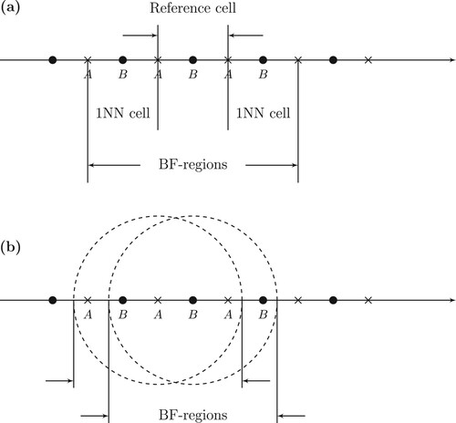
In the recent work by Røeggen and Gao [5] a basis function (BF) region is defined as a unit cell and a certain number of nearest neighbour unit cells. However, since we in this work advocate spherical embedding, the BF-region of an atom comprizes the atom in question and all its partner atoms in a sphere centred on the nucleus of the atom. The number of atoms of the BF-region is denoted $N_{\mathrm{B}\mathrm{F}}^A$. See illustraction in Figure 1. Two different atom-centred basis sets are associated with each nucleus, a large one, $\{{\chi }_{\mu }^{A,\mathrm{l}\mathrm{b}};\mu =1,\dots ,m_A^{\mathrm{l}\mathrm{b}}\}$, and a small one, $\{{\chi }_{\mu }^{A,\mathrm{s}\mathrm{b}};\mu =1,\dots ,m_A^{\mathrm{s}\mathrm{b}}\}$. The basis set for an atom in the unit cell is then (16) $\begin{array}{rl}{\mathrm{\Omega }}_{\mathrm{d}\mathrm{u}\mathrm{a}\mathrm{l}}^A& =\{{\chi }_{\mu }^{A,\mathrm{d}\mathrm{u}\mathrm{a}\mathrm{l}};\mu =1,\dots ,m_A^{\mathrm{d}\mathrm{u}\mathrm{a}\mathrm{l}}\}\\ & =\{{\chi }_{\mu }^{A,\mathrm{l}\mathrm{b}};\mu =1,\dots ,m_A^{\mathrm{l}\mathrm{b}}\}\\ & \bigcup _{B\in {\mathrm{\Omega }}_{\mathrm{B}\mathrm{F}}^A}\{{\chi }_{\mu }^{B,\mathrm{s}\mathrm{b}};\mu =1,\dots ,m_B^{\mathrm{s}\mathrm{b}}\},\end{array}$(16) where ${\mathrm{\Omega }}_{\mathrm{B}\mathrm{F}}^A$ is the set of atoms in the BF-region (excluding atom A).

Figure 1. Two different models of infinite, one-dimensional periodic systems of unit cells. (a) Fixed number of unit cells. (b) Spherical embedding.

The spatial part of a spin orbital (α- or β-type): (17) ${\psi }_i^A=\sum _{\mu =1}^{m_A^{\mathrm{d}\mathrm{u}\mathrm{a}\mathrm{l}}}{U}_{\mu ,i}^{\mathrm{d}\mathrm{u}\mathrm{a}\mathrm{l}}{\chi }_{\mu }^{A,\mathrm{d}\mathrm{u}\mathrm{a}\mathrm{l}}.$(17) The orbitals of the UHF wave functions are subjected to orthogonality constraints: (18) $\begin{array}{rl}〈{\psi }_i^{A,\alpha }|{\psi }_j^{B,\alpha }〉& ={\delta }_{ij}{\delta }_{AB},\end{array}$(18) (19) $\begin{array}{rl}〈{\psi }_i^{A,\text{β}}|{\psi }_j^{B,\text{β}}〉& ={\delta }_{ij}{\delta }_{AB}.\end{array}$(19) The constraints, Equations (18(18) $\begin{array}{rl}〈{\psi }_i^{A,\alpha }|{\psi }_j^{B,\alpha }〉& ={\delta }_{ij}{\delta }_{AB},\end{array}$(18) ) and (19(19) $\begin{array}{rl}〈{\psi }_i^{A,\text{β}}|{\psi }_j^{B,\text{β}}〉& ={\delta }_{ij}{\delta }_{AB}.\end{array}$(19) ), require special attention in the optimisation procedure since the orbitals of different atoms are expressed in different basis sets.

2.3. Orbital localisation measures

To describe orbital localisation, we use charge centroids and charge ellipsoids [22] in this work. As illustrated in our previous work [4], it is a very compact and visual way of looking at orbital localisation. The charge centroid is defined as (20) ${\mathit{r}}^C=〈\psi |\mathit{r}\psi 〉,$(20) where ψ is any spatial orbital.

The extension or spread of an orbital can be described by the second-order variance matrix (21) $M_{rs}=〈\psi |(x_r-x_r^C)(x_s-x_s^C)\psi 〉,r,s\in \{1,2,3\},$(21) where $x_r^C$ is the rth component of the charge centroid vector ${\mathit{r}}^C$. Diagonalization of the second-order variance matrix $M_{rs}$ yields the charge ellipsoid.

The eigenvalues $\{a_1,a_2,a_3\}$ of the matrix $M_{rs}$ correspond to the squares of the half-axes of the ellipsoid. The standard deviations in three orthogonal directions, i.e. the directions of the half-axes, are therefore given by (22) $\mathrm{\Delta }{l}_i=a_i^{1/2},i\in \{1,2,3\},$(22) which can be used as a measure of the extension of the orbital with respect to the charge centroid position. We may also use the volume of the ellipsoid $V=\frac{4}{3}\pi \mathrm{\Delta }{l}_1\mathrm{\Delta }{l}_2\mathrm{\Delta }{l}_3$ as a single number for the extension.

The half-axes also define a lower bound for the kinetic energy associated with a given orbital ψ: (23) $E_{\mathrm{k}\mathrm{i}\mathrm{n}}=〈\psi |-\frac{1}{2}{\mathrm{\nabla }}^2\psi 〉\ge \frac{1}{8}[\frac{1}{(\mathrm{\Delta }{l}_1{)}^2}+\frac{1}{(\mathrm{\Delta }{l}_2{)}^2}+\frac{1}{(\mathrm{\Delta }{l}_3{)}^2}].$(23) This inequality can be derived from the Heisenberg uncertainty principle [4] and expresses neatly that the kinetic energy increases when an orbital becomes more compact.

3. The physical model for a periodic system

In the physical model for constructing the orbitals of the UHF function we include as a constraint that all atoms of the same type should be described by identical orbitals, i.e. translational symmetry should be satisfied. Hence, there are no surface effects in the physical model. In Figure 1 we consider a one-dimensional system with two different atoms in the unit cell. We look at two different types of embedding. The first one, (a), is an embedding with a fixed number of unit cells. In Figure 1, embedding (a) consists of the reference cell and the two first nearest neighbouring cells (1NN). The second embedding is a spherical one including all atoms in sphere surrounding an atom of the reference cell. In Figure 1, the radius of the sphere is slightly larger than the unit cell distance.

When we optimise the UHF orbitals, we consider an effective Hamiltonian for each atom in the reference cell. The Hamiltonian includes only the atoms of the BF-region. We notice that for embedding (a), the atom A of the reference cell has two atoms on the left and three atoms on the right, and vice versa for atom B. This lack of symmetry creates an artificial shift of the charge density. For a one-dimensional system this shift can be reduced by including a large number of unit cells in the BF-region. However, for atoms in three-dimensional lattices, such an extension is not feasible. On the other hand, if we look at spherical embedding, Figure 1(b), we have perfect symmetry for any size of the embedding.

4. Computational aspects

The computational feasibility of a model is of paramount importance when we consider large complexes such as a metal. In the first subsection we shall give details on the procedure for obtaining the spin orbitals of the UHF wave function. The second and the third subsections are devoted to the electron correlation problem restricted to intra-atomic and diatomic terms. In particular the diatomic terms need careful considerations. We have to compute of the order 1000 diatomic terms for obtaining sufficiently converged results. Hence, a simplistic, but still fairly accurate, procedure has to be constructed.

4.1. Determination of the UHF orbitals

The starting point for the UHF procedure is an effective Hamiltonian for an atom A of the reference unit cell: (24) ${\mathbf{H}}_{\mathrm{e}\mathrm{f}\mathrm{f}}^A=\sum _{i=1}^{N_A}{\mathbf{h}}_{\mathrm{e}\mathrm{f}\mathrm{f}}^A\left({\mathit{r}}_i\right)+\sum _{i<j}^{N_A}\frac{1}{r_{ij}},$(24) where the effective one-electron Hamiltonian is given by (25) ${\mathbf{h}}_{\mathrm{e}\mathrm{f}\mathrm{f}}^A\left({\mathit{r}}_i\right)=\mathbf{h}\left({\mathit{r}}_i\right)+\sum _{B\in {\mathrm{\Omega }}_{\mathrm{B}\mathrm{F}}^A}^{N_{\mathrm{a}\mathrm{t}\mathrm{o}\mathrm{m}\mathrm{s}}}\sum _{j=1}^{N_B}(J_j^B-K_j^B).$(25) $N_A$ and $N_B$ are the number of electrons of atoms A and B, respectively. $J_j^B$ and $K_j^B$ are the Coulomb and exchange operators generated by the spin orbital ${\psi }_j^B$ of atom B, and $\mathbf{h}\left({\mathit{r}}_i\right)$ is the one-electron operator for the complex: atom $A+{\mathrm{\Omega }}_{\mathrm{B}\mathrm{F}}^A$, i.e. (26) $\mathbf{h}\left({\mathit{r}}_i\right)=-\frac{1}{2}{\mathrm{\nabla }}_i^2-\frac{Z_A}{|{\mathit{R}}_A-{\mathit{r}}_i|}-\sum _{B\in {\mathrm{\Omega }}_{\mathrm{B}\mathrm{F}}^A}\frac{Z_B}{|{\mathit{R}}_B-{\mathit{r}}_i|}.$(26) In Equation (26(26) $\mathbf{h}\left({\mathit{r}}_i\right)=-\frac{1}{2}{\mathrm{\nabla }}_i^2-\frac{Z_A}{|{\mathit{R}}_A-{\mathit{r}}_i|}-\sum _{B\in {\mathrm{\Omega }}_{\mathrm{B}\mathrm{F}}^A}\frac{Z_B}{|{\mathit{R}}_B-{\mathit{r}}_i|}.$(26) ), the symbols have their conventional meaning. The spin orbitals of the atom A are orthogonal to all spin orbitals of the atoms in the set ${\mathrm{\Omega }}_{\mathrm{B}\mathrm{F}}^A$, i.e. (27) $\begin{array}{rl}& 〈{\psi }_i^A|{\psi }_j^B〉=0,1\le i\le N_A,B\in {\mathrm{\Omega }}_{\mathrm{B}\mathrm{F}}^A,\\ & 1\le j\le N_B.\end{array}$(27) In order to comply with the orthogonality constraints of Equation (27(27) $\begin{array}{rl}& 〈{\psi }_i^A|{\psi }_j^B〉=0,1\le i\le N_A,B\in {\mathrm{\Omega }}_{\mathrm{B}\mathrm{F}}^A,\\ & 1\le j\le N_B.\end{array}$(27) ), and the translational symmetry of the orbitals, the optimisation procedure consists of several iterative steps.

Preliminary calculations on one-dimensional systems of pure metals demonstrate that the localised orbitals are slightly perturbed atomic orbitals. The PATMOS basis set procedure with a large and a small basis sets assigned to each atom, is particularly well-suited to deal with this feature. The large basis set can easily account for the small expansion of the atomic density while the small basis set for the partner atoms in ${\mathrm{\Omega }}_{\mathrm{B}\mathrm{F}}^A$ takes care of the orthogonality constraints. However, we can introduce a further simplification. Let $P_{\mathrm{o}\mathrm{c}\mathrm{c}}^{B,\alpha }$ denote the projection operator associated with the α-type spin orbitals of an atom B in the BF-region of atom A. The dual space of atom A, Equation (16(16) $\begin{array}{rl}{\mathrm{\Omega }}_{\mathrm{d}\mathrm{u}\mathrm{a}\mathrm{l}}^A& =\{{\chi }_{\mu }^{A,\mathrm{d}\mathrm{u}\mathrm{a}\mathrm{l}};\mu =1,\dots ,m_A^{\mathrm{d}\mathrm{u}\mathrm{a}\mathrm{l}}\}\\ & =\{{\chi }_{\mu }^{A,\mathrm{l}\mathrm{b}};\mu =1,\dots ,m_A^{\mathrm{l}\mathrm{b}}\}\\ & \bigcup _{B\in {\mathrm{\Omega }}_{\mathrm{B}\mathrm{F}}^A}\{{\chi }_{\mu }^{B,\mathrm{s}\mathrm{b}};\mu =1,\dots ,m_B^{\mathrm{s}\mathrm{b}}\},\end{array}$(16) ), is modified in the follwing way: (28) ${\hat{\chi }}_{\mu }^{A,\mathrm{d}\mathrm{u}\mathrm{a}\mathrm{l}}=(1-\sum _{B\in {\mathrm{\Omega }}_{\mathrm{B}\mathrm{F}}^A}{P}_{\mathrm{o}\mathrm{c}\mathrm{c}}^{B,\alpha }){\chi }_{\mu }^{A,\mathrm{d}\mathrm{u}\mathrm{a}\mathrm{l}},1\le \mu \le m_A^{\mathrm{d}\mathrm{u}\mathrm{a}\mathrm{l}}.$(28) A linear independent set of functions, $\{{\varphi }_{\mu }^{A,\alpha };1\le \mu \le {\tilde{m}}_A^{\mathrm{d}\mathrm{u}\mathrm{a}\mathrm{l}}\le m_A^{\mathrm{d}\mathrm{u}\mathrm{a}\mathrm{l}}\}$, is constructed from the functions defined in Equation (28(28) ${\hat{\chi }}_{\mu }^{A,\mathrm{d}\mathrm{u}\mathrm{a}\mathrm{l}}=(1-\sum _{B\in {\mathrm{\Omega }}_{\mathrm{B}\mathrm{F}}^A}{P}_{\mathrm{o}\mathrm{c}\mathrm{c}}^{B,\alpha }){\chi }_{\mu }^{A,\mathrm{d}\mathrm{u}\mathrm{a}\mathrm{l}},1\le \mu \le m_A^{\mathrm{d}\mathrm{u}\mathrm{a}\mathrm{l}}.$(28) ). The next step is to project the large basis set, $\{{\chi }_{\mu }^{A,lb};1\le \mu \le m_A^{lb}\}$, onto the modified dual set. The perturbed large basis set is denoted $\{{\tilde{\chi }}_{\mu }^{A,lb;\alpha };1\le \mu \le m_A^{lb}\}$. By construction this modified basis is orthogonal to all α-type orbitals of the atoms of ${\mathrm{\Omega }}_{\mathrm{B}\mathrm{F}}^A$. A similar procedure yields $\{{\tilde{\chi }}_{\mu }^{A,lb;\text{β}};1\le \mu \le m_A^{lb}\}$.

The next step is to solve the Hartree-Fock equations for atom A: (29) $F_A^{\alpha }{\psi }_i^{A,\alpha }={ϵ}_i^{A,\alpha }{\psi }_i^{A,\alpha },$(29) and (30) $F_A^{\text{β}}{\psi }_i^{A,\text{β}}={ϵ}_i^{A,\text{β}}{\psi }_i^{A,\text{β}}.$(30) The orbitals are expressed in terms of the modified large basis sets, i.e. (31) ${\psi }_i^{A,\alpha }=\sum _{\mu =1}^{m_A^{\mathrm{l}\mathrm{b}}}{U}_{\mu }^{A,\alpha }{\tilde{\chi }}_{\mu }^{A,\mathrm{l}\mathrm{b};\alpha },$(31) and (32) ${\psi }_i^{A,\text{β}}=\sum _{\mu =1}^{m_A^{\mathrm{l}\mathrm{b}}}{U}_{\mu }^{A,\text{β}}{\tilde{\chi }}_{\mu }^{A,\mathrm{l}\mathrm{b};\text{β}}.$(32) A fixed-point iteration procedure does not necessarily converge. Hence, we introduce a UHF functional (33) $E_{\mathrm{u}\mathrm{c}}^{\mathrm{U}\mathrm{H}\mathrm{F}}=\sum _{A=1}^{N_{\mathrm{a}\mathrm{t}\mathrm{o}\mathrm{m}\mathrm{s}}^{\mathrm{u}\mathrm{c}}}{E}_A^{\mathrm{U}\mathrm{H}\mathrm{F},\mathrm{e}\mathrm{f}\mathrm{f}},$(33) where (34) $E_A^{\mathrm{U}\mathrm{H}\mathrm{F},\mathrm{e}\mathrm{f}\mathrm{f}}=E_A^{\mathrm{U}\mathrm{H}\mathrm{F}}+\frac{1}{2}\sum _{B\in {\mathrm{\Omega }}_{\mathrm{B}\mathrm{F}}^A}(E_{AB}^{\mathrm{C}\mathrm{o}\mathrm{u}\mathrm{l}}+E_{AB}^{\mathrm{e}\mathrm{x}\mathrm{c}\mathrm{h}}).$(34) Let $\left\{{\psi }_i^{A,\mathrm{o}\mathrm{l}\mathrm{d}}\right\}$ denote the spin orbitals of the previous iteration, and $\left\{{\psi }_i^{A,\mathrm{n}\mathrm{e}\mathrm{w}}\right\}$ the spin orbitals of the last one. Then we minimise the functional $E_{\mathrm{u}\mathrm{c}}^{\mathrm{U}\mathrm{H}\mathrm{F}}$ with respect to the length of the orbital correction: (35) $\begin{array}{rl}{\psi }_i^A\left(\lambda \right)& ={\psi }_i^{A,\mathrm{o}\mathrm{l}\mathrm{d}}+\lambda ({\psi }_i^{A,\mathrm{n}\mathrm{e}\mathrm{w}}-{\psi }_i^{A,\mathrm{o}\mathrm{l}\mathrm{d}}),\\ & 1\le A\le N_{\mathrm{a}\mathrm{t}\mathrm{o}\mathrm{m}\mathrm{s}}^{\mathrm{u}\mathrm{c}},1\le i\le N_A,0<\lambda \le 1.\end{array}$(35) The orbitals $\left\{{\psi }_i^A\right(\lambda \left)\right\}$ have to be properly symmetrised. The procedure is described in Appendix. We denote the symmetrised orbitals $\left\{{\psi }_i^{A,\mathrm{s}\mathrm{y}\mathrm{m}}\right(\lambda \left)\right\}$.

If (36) $E_{\mathrm{u}\mathrm{c}}^{\mathrm{U}\mathrm{H}\mathrm{F}}\left(\left\{{\psi }_i^{A,\mathrm{s}\mathrm{y}\mathrm{m}}\right(\lambda \left)\right\}\right)<E_{\mathrm{u}\mathrm{c}}^{\mathrm{U}\mathrm{H}\mathrm{F}}\left(\left\{{\psi }_i^{A,\mathrm{o}\mathrm{l}\mathrm{d}}\right\}\right),$(36) then we continue to the next iteration. Otherwise, we choose new values of λ until we can perform a parabolic fit. Two or three values of λ are in most cases sufficient. To obtain a converged result of accuracy ${10}^{-7}$ Hartree, typically 15–20 iterations are required.

4.2. Correlation energy

Typically, intra-atomic MP2 energy yields 80–90% of the corresponding full configuration interation (FCI) energy. The intra-atomic MP2 energy for lithium varies only slightly for different values of the lattice parameter, i.e. less than 1%. Hence, MP2 should be sufficiently accurate for our purpose.

The inter-atomic correlation terms are more demanding. In this work we are using both MP2 and second-order Epstein-Nesbet (EN2) theory. MP2 underestimates the inter-atomic correlation enery while EN2 usually overestimates it.

4.2.1. Intra-atomic correlation energy

Let $\{{\psi }_i^A;1\le i\le 2m_A^{\mathrm{l}\mathrm{b}}\}$ denote the spin orbitals obtained by solving the Hartree-Fock equations, Equations (29(29) $F_A^{\alpha }{\psi }_i^{A,\alpha }={ϵ}_i^{A,\alpha }{\psi }_i^{A,\alpha },$(29) ) and (30(30) $F_A^{\text{β}}{\psi }_i^{A,\text{β}}={ϵ}_i^{A,\text{β}}{\psi }_i^{A,\text{β}}.$(30) ), and $\{{ϵ}_i^A;1\le i\le 2m_A^{\mathrm{l}\mathrm{b}}\}$ the corresponding orbital energies. The intra-atomic correlation for atom A is then approximated by the standard MP2 expression: (37) $E_A^{\mathrm{M}\mathrm{P}2}=\sum _{i<j}^{\mathrm{o}\mathrm{c}\mathrm{c}}\sum _{r<s}^{\mathrm{v}\mathrm{i}\mathrm{r}\mathrm{t}}\frac{\begin{array}{c}|〈{\psi }_i^A{\psi }_j^A|g{\psi }_r^A{\psi }_s^A〉\\ -{〈{\psi }_i^A{\psi }_j^A|g{\psi }_s^A{\psi }_r^A〉|}^2\end{array}}{{ϵ}_i^A+{ϵ}_j^A-{ϵ}_r^A-{ϵ}_s^A},$(37) where the two sums are restricted to respectively occupied and virtual spin orbitals. By distinguishing between α- and β-type spin orbitals, the MP2 energy can be written as a sum of three different terms: (38) $E_A^{\mathrm{M}\mathrm{P}2}=E_A^{\mathrm{M}\mathrm{P}2;\alpha \alpha }+E_A^{\mathrm{M}\mathrm{P}2;\text{β}\text{β}}+E_A^{\mathrm{M}\mathrm{P}2;\alpha \text{β}}.$(38)

4.2.2. Inter-atomic correlation energy

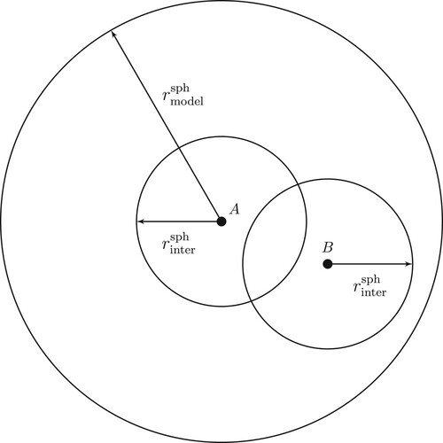
For atom A we calculate the diatomic correlation terms for all atoms with a sphere of radius $r_{\mathrm{m}\mathrm{o}\mathrm{d}\mathrm{e}\mathrm{l}}^{\mathrm{s}\mathrm{p}\mathrm{h}}$ surrounding the nucleus of A. The radius of the sphere is determinde by a selected convergence criterion. For a pair of atoms $(A,B)$ we define inter-atomic embedding ${\mathrm{\Omega }}_{\mathrm{i}\mathrm{n}\mathrm{t}\mathrm{e}\mathrm{r}}^A$ and ${\mathrm{\Omega }}_{\mathrm{i}\mathrm{n}\mathrm{t}\mathrm{e}\mathrm{r}}^B$. The embedding ${\mathrm{\Omega }}_{\mathrm{i}\mathrm{n}\mathrm{t}\mathrm{e}\mathrm{r}}^A$ includes all atoms within a sphere of radius $r_{\mathrm{i}\mathrm{n}\mathrm{t}\mathrm{e}\mathrm{r}}^{\mathrm{s}\mathrm{p}\mathrm{h}}$ surrounding the nucleus of atom A (but excluding atom A). Similarly for atom B. The embedding for the pair $(A,B)$ is then (see Figure 2) (39) ${\mathrm{\Omega }}_{\mathrm{i}\mathrm{n}\mathrm{t}\mathrm{e}\mathrm{r}}^{AB}={\mathrm{\Omega }}_{\mathrm{i}\mathrm{n}\mathrm{t}\mathrm{e}\mathrm{r}}^A\cup {\mathrm{\Omega }}_{\mathrm{i}\mathrm{n}\mathrm{t}\mathrm{e}\mathrm{r}}^B-{\mathrm{\Omega }}_{\mathrm{i}\mathrm{n}\mathrm{t}\mathrm{e}\mathrm{r}}^A\cap {\mathrm{\Omega }}_{\mathrm{i}\mathrm{n}\mathrm{t}\mathrm{e}\mathrm{r}}^B.$(39)

Figure 2. Different embeddings. The largest sphere with radices $r_{\mathrm{m}\mathrm{o}\mathrm{d}\mathrm{e}\mathrm{l}}^{\mathrm{s}\mathrm{p}\mathrm{h}}$ includes all atoms B interacting with atom A. The smaller spheres surrounding A and B define the embedding used in calculating the interaction between atoms A and B.

The effective Hamiltonian for the pair $(A,B)$ is (40) $H_{\mathrm{e}\mathrm{f}\mathrm{f}}^{AB}=\sum _{i=1}^{N_A+N_B}{h}_{\mathrm{e}\mathrm{f}\mathrm{f}}^{AB}\left(r_i\right)+\sum _{i<j}^{N_A+N_B}\frac{1}{r_{ij}},$(40) where (41) $\begin{array}{rl}{h}_{\mathrm{e}\mathrm{f}\mathrm{f}}^{AB}\left(r_i\right)& =-\frac{1}{2}{\mathrm{\nabla }}^2-\frac{Z_A}{|{\mathit{R}}_A-{\mathit{r}}_i|}-\frac{Z_B}{|{\mathit{R}}_B-{\mathit{r}}_i|}\\ & -\sum _{C\in {\mathrm{\Omega }}_{\mathrm{i}\mathrm{n}\mathrm{t}\mathrm{e}\mathrm{r}}^{AB}}[\frac{Z_C}{|{\mathit{R}}_C-{\mathit{r}}_i|}+\sum _{j=1}^{N_C}(J_j^C-K_j^C)].\end{array}$(41) In Equation (41(41) $\begin{array}{rl}{h}_{\mathrm{e}\mathrm{f}\mathrm{f}}^{AB}\left(r_i\right)& =-\frac{1}{2}{\mathrm{\nabla }}^2-\frac{Z_A}{|{\mathit{R}}_A-{\mathit{r}}_i|}-\frac{Z_B}{|{\mathit{R}}_B-{\mathit{r}}_i|}\\ & -\sum _{C\in {\mathrm{\Omega }}_{\mathrm{i}\mathrm{n}\mathrm{t}\mathrm{e}\mathrm{r}}^{AB}}[\frac{Z_C}{|{\mathit{R}}_C-{\mathit{r}}_i|}+\sum _{j=1}^{N_C}(J_j^C-K_j^C)].\end{array}$(41) ), the symbols have their standard meaning. The Coulomb and exchange operators in Equation (41(41) $\begin{array}{rl}{h}_{\mathrm{e}\mathrm{f}\mathrm{f}}^{AB}\left(r_i\right)& =-\frac{1}{2}{\mathrm{\nabla }}^2-\frac{Z_A}{|{\mathit{R}}_A-{\mathit{r}}_i|}-\frac{Z_B}{|{\mathit{R}}_B-{\mathit{r}}_i|}\\ & -\sum _{C\in {\mathrm{\Omega }}_{\mathrm{i}\mathrm{n}\mathrm{t}\mathrm{e}\mathrm{r}}^{AB}}[\frac{Z_C}{|{\mathit{R}}_C-{\mathit{r}}_i|}+\sum _{j=1}^{N_C}(J_j^C-K_j^C)].\end{array}$(41) ) require special attention. For each pair of atoms $(A,B)$, the proper calculation of two-electron integrals requires three sets of dual basis sets as defined in Equation (16(16) $\begin{array}{rl}{\mathrm{\Omega }}_{\mathrm{d}\mathrm{u}\mathrm{a}\mathrm{l}}^A& =\{{\chi }_{\mu }^{A,\mathrm{d}\mathrm{u}\mathrm{a}\mathrm{l}};\mu =1,\dots ,m_A^{\mathrm{d}\mathrm{u}\mathrm{a}\mathrm{l}}\}\\ & =\{{\chi }_{\mu }^{A,\mathrm{l}\mathrm{b}};\mu =1,\dots ,m_A^{\mathrm{l}\mathrm{b}}\}\\ & \bigcup _{B\in {\mathrm{\Omega }}_{\mathrm{B}\mathrm{F}}^A}\{{\chi }_{\mu }^{B,\mathrm{s}\mathrm{b}};\mu =1,\dots ,m_B^{\mathrm{s}\mathrm{b}}\},\end{array}$(16) ): ${\mathrm{\Omega }}_{\mathrm{d}\mathrm{u}\mathrm{a}\mathrm{l}}^A$, ${\mathrm{\Omega }}_{\mathrm{d}\mathrm{u}\mathrm{a}\mathrm{l}}^B$ and ${\mathrm{\Omega }}_{\mathrm{d}\mathrm{u}\mathrm{a}\mathrm{l}}^C$. Since the number of atoms in ${\mathrm{\Omega }}_{\mathrm{i}\mathrm{n}\mathrm{t}\mathrm{e}\mathrm{r}}^{AB}$ is of the order of the sum of atoms in the sets ${\mathrm{\Omega }}_{\mathrm{B}\mathrm{F}}^A$ and ${\mathrm{\Omega }}_{\mathrm{B}\mathrm{F}}^B$, the computational cost of this proper approach is prohibitively high. Our simplistic procedure is based on the fact that the charge ellipsoids [4] associated with the occupied orbitals are spherical symmetric. Hence, we project the orbitals $\{{\psi }_i^C;1\le i\le N_C\}$ onto the small basis set $\{{\chi }_{\mu }^{C;\mathrm{s}\mathrm{b}};1\le \mu \le m_C^{\mathrm{s}\mathrm{b}}\}$: (42) $\begin{array}{rl}{\psi }_i^{C;\mathrm{s}\mathrm{b},\alpha }& =\sum _{\mu =1}^{m_C^{\mathrm{s}\mathrm{b}}}{\chi }_{\mu }^{C;\mathrm{s}\mathrm{b}}{U}_{\mu ,i}^{C;\mathrm{s}\mathrm{b},\alpha },\end{array}$(42) (43) $\begin{array}{rl}{\psi }_i^{C;\mathrm{s}\mathrm{b},\text{β}}& =\sum _{\mu =1}^{m_C^{\mathrm{s}\mathrm{b}}}{\chi }_{\mu }^{C;\mathrm{s}\mathrm{b}}{U}_{\mu ,i}^{C;\mathrm{s}\mathrm{b},\text{β}}.\end{array}$(43) Accordingly, by using $\left\{{\psi }_i^{C;\mathrm{s}\mathrm{b},\alpha }\right\}$ and $\left\{{\psi }_i^{C;\mathrm{s}\mathrm{b},\text{β}}\right\}$ in calculating the matrix elements of the operators $J_j^C$ and $K_j^C$ in Equation (41(41) $\begin{array}{rl}{h}_{\mathrm{e}\mathrm{f}\mathrm{f}}^{AB}\left(r_i\right)& =-\frac{1}{2}{\mathrm{\nabla }}^2-\frac{Z_A}{|{\mathit{R}}_A-{\mathit{r}}_i|}-\frac{Z_B}{|{\mathit{R}}_B-{\mathit{r}}_i|}\\ & -\sum _{C\in {\mathrm{\Omega }}_{\mathrm{i}\mathrm{n}\mathrm{t}\mathrm{e}\mathrm{r}}^{AB}}[\frac{Z_C}{|{\mathit{R}}_C-{\mathit{r}}_i|}+\sum _{j=1}^{N_C}(J_j^C-K_j^C)].\end{array}$(41) ), the number of two-electron integrals are restricted to the basis sets $\{{\chi }_{\mu }^{A;\mathrm{l}\mathrm{b}};1\le \mu \le m_A^{\mathrm{l}\mathrm{b}}\}\cup \{{\chi }_{\mu }^{B;\mathrm{l}\mathrm{b}};1\le \mu \le m_B^{\mathrm{l}\mathrm{b}}\}$ plus the small basis sets for the atoms in ${\mathrm{\Omega }}_{\mathrm{i}\mathrm{n}\mathrm{t}\mathrm{e}\mathrm{r}}^{AB}$.

The virtual orbitals to be used in the diatomic correlation treatment are derived from the intra-atomic calculations. For both α and β orbitals we go through the following steps. A symmetric orthonormalization of $\{{\psi }_a^{A;\mathrm{v}\mathrm{i}\mathrm{r}\mathrm{t}};1\le a\le m_A^{\mathrm{v}\mathrm{i}\mathrm{r}\mathrm{t}}\}\cup \{{\psi }_b^{B;\mathrm{v}\mathrm{i}\mathrm{r}\mathrm{t}};1\le b\le m_B^{\mathrm{v}\mathrm{i}\mathrm{r}\mathrm{t}}\}$ yields $\{{\varphi }_r^{ab;\mathrm{v}\mathrm{i}\mathrm{r}\mathrm{t}};1\le r\le m_A^{\mathrm{v}\mathrm{i}\mathrm{r}\mathrm{t}}+m_B^{\mathrm{v}\mathrm{i}\mathrm{r}\mathrm{t}}\}$. If atom $B\in {\mathrm{\Omega }}_{\mathrm{B}\mathrm{F}}^A$, then the occupied orbitals of atom B are by construction orthogonal to the occupied orbitals of atom A [see Equation (27(27) $\begin{array}{rl}& 〈{\psi }_i^A|{\psi }_j^B〉=0,1\le i\le N_A,B\in {\mathrm{\Omega }}_{\mathrm{B}\mathrm{F}}^A,\\ & 1\le j\le N_B.\end{array}$(27) )]. If $B\notin {\mathrm{\Omega }}_{\mathrm{B}\mathrm{F}}^A$, then the orthogonality condition is not necessarily fulfilled. Consequently, we perform a symmetric orthonormalization of the occupied orbitals. This is followed by a Gram-Schmidt orthonormalization of occupied plus virtual orbitals. The orbitals are appropriately divided in three separate groups – for α-type orbitals, $\{{\psi }_i^{A;\mathrm{o}\mathrm{c}\mathrm{c};\alpha };1\le i\le N_A^{\alpha }\}$, $\{{\psi }_j^{B;\mathrm{o}\mathrm{c}\mathrm{c};\alpha };1\le j\le N_B^{\alpha }\}$ and $\{{\psi }_r^{AB;\mathrm{v}\mathrm{i}\mathrm{r}\mathrm{t};\alpha };1\le r\le m_A^{\mathrm{v}\mathrm{i}\mathrm{r}\mathrm{t}}+m_B^{\mathrm{v}\mathrm{i}\mathrm{r}\mathrm{t}}=m_{AB}^{\mathrm{v}\mathrm{i}\mathrm{r}\mathrm{t}}\}$. If $F_{AB}^{\alpha }$ denotes the α-type Fock operator for the atom pair $(A,B)$, we define (44) $\begin{array}{rl}{ϵ}_i^{A;\mathrm{o}\mathrm{c}\mathrm{c};\alpha }& =〈{\psi }_i^{A;\mathrm{o}\mathrm{c}\mathrm{c};\alpha }|F_{AB}^{\alpha }{\psi }_i^{A;\mathrm{o}\mathrm{c}\mathrm{c};\alpha }〉,\end{array}$(44) (45) $\begin{array}{rl}{ϵ}_j^{B;\mathrm{o}\mathrm{c}\mathrm{c};\alpha }& =〈{\psi }_j^{B;\mathrm{o}\mathrm{c}\mathrm{c};\alpha }|F_{AB}^{\alpha }{\psi }_j^{B;\mathrm{o}\mathrm{c}\mathrm{c};\alpha }〉.\end{array}$(45) The virtual orbitals correspond to a diagonal block of the Fock operator, i.e. (46) $〈{\psi }_r^{AB;\mathrm{v}\mathrm{i}\mathrm{r}\mathrm{t};\alpha }|F_{AB}^{\alpha }{\psi }_s^{AB;\mathrm{v}\mathrm{i}\mathrm{r}\mathrm{t};\alpha }〉={\delta }_{rs}{ϵ}_r^{AB;\mathrm{v}\mathrm{i}\mathrm{r}\mathrm{t};\alpha }.$(46) By using spin orbitals the diatomic MP2 energy can be written as (47) $E_{AB}^{\mathrm{M}\mathrm{P}2}=\sum _{i=1}^{N_A}\sum _{j=1}^{N_B}\sum _{r<s}^{m_{AB}^{\mathrm{v}\mathrm{i}\mathrm{r}\mathrm{t}}}\frac{\begin{array}{c}|〈{\psi }_i^A{\psi }_j^B|g{\psi }_r^{AB}{\psi }_s^{AB}〉\\ -{〈{\psi }_i^A{\psi }_j^B|g{\psi }_s^{AB}{\psi }_r^{AB}〉|}^2\end{array}}{\begin{array}{c}{ϵ}_i^{A;\mathrm{o}\mathrm{c}\mathrm{c}}+{ϵ}_j^{B;\mathrm{o}\mathrm{c}\mathrm{c}}\\ -{ϵ}_r^{AB;\mathrm{v}\mathrm{i}\mathrm{r}\mathrm{t}}-{ϵ}_s^{AB;\mathrm{v}\mathrm{i}\mathrm{r}\mathrm{t}}\end{array}}.$(47) The MP2 energy can be partioned into a sum of four terms when we distinguish between α and β spin orbitals: (48) $E_{AB}^{\mathrm{M}\mathrm{P}2}=E_{AB}^{\mathrm{M}\mathrm{P}2;\alpha \alpha }+E_{AB}^{\mathrm{M}\mathrm{P}2;\text{β}\text{β}}+E_{AB}^{\mathrm{M}\mathrm{P}2;\alpha \text{β}}+E_{AB}^{\mathrm{M}\mathrm{P}2;\text{β}\alpha }.$(48) As for the Epstein-Nesbet correction we introduce a two-electron Hamiltonian related to the spin orbitals ${\psi }_i^A$ and ${\psi }_j^B$ (49) $H_{\mathrm{e}\mathrm{f}\mathrm{f}}^{A,i;B,j}(r_1,r_2)=h_{\mathrm{e}\mathrm{f}\mathrm{f}}^{A,i;B,j}\left(r_1\right)+h_{\mathrm{e}\mathrm{f}\mathrm{f}}^{A,i;B,j}\left(r_2\right)+\frac{1}{r_{12}},$(49) where (50) $\begin{array}{rl}{h}_{\mathrm{e}\mathrm{f}\mathrm{f}}^{A,i;B,j}\left(r\right)& =h_{\mathrm{e}\mathrm{f}\mathrm{f}}^{AB}\left(r\right)+\sum _{i_A\ne i}^{N_A}(J_{i_A}^A-K_{i_A}^A)\\ & +\sum _{j_B\ne j}^{N_B}(J_{j_B}^B-K_{j_B}^B),\end{array}$(50) and $h_{\mathrm{e}\mathrm{f}\mathrm{f}}^{AB}\left(r\right)$ is defined in Equation (41(41) $\begin{array}{rl}{h}_{\mathrm{e}\mathrm{f}\mathrm{f}}^{AB}\left(r_i\right)& =-\frac{1}{2}{\mathrm{\nabla }}^2-\frac{Z_A}{|{\mathit{R}}_A-{\mathit{r}}_i|}-\frac{Z_B}{|{\mathit{R}}_B-{\mathit{r}}_i|}\\ & -\sum _{C\in {\mathrm{\Omega }}_{\mathrm{i}\mathrm{n}\mathrm{t}\mathrm{e}\mathrm{r}}^{AB}}[\frac{Z_C}{|{\mathit{R}}_C-{\mathit{r}}_i|}+\sum _{j=1}^{N_C}(J_j^C-K_j^C)].\end{array}$(41) ). The Coulomb and exchange operators in Equation (50(50) $\begin{array}{rl}{h}_{\mathrm{e}\mathrm{f}\mathrm{f}}^{A,i;B,j}\left(r\right)& =h_{\mathrm{e}\mathrm{f}\mathrm{f}}^{AB}\left(r\right)+\sum _{i_A\ne i}^{N_A}(J_{i_A}^A-K_{i_A}^A)\\ & +\sum _{j_B\ne j}^{N_B}(J_{j_B}^B-K_{j_B}^B),\end{array}$(50) ) have their conventional meaning.

By introducing the following set of two-electron functions (51) $\begin{array}{rl}{\mathrm{\Phi }}_o^{ij}& =det\left|{\psi }_i^A{\psi }_j^B\right|,\end{array}$(51) (52) $\begin{array}{rl}{\mathrm{\Phi }}_{rs}& =det\left|{\psi }_r^{AB;\mathrm{v}\mathrm{i}\mathrm{r}\mathrm{t}}{\psi }_s^{AB;\mathrm{v}\mathrm{i}\mathrm{r}\mathrm{t}}\right|,1\le r,s\le m_{AB}^{\mathrm{v}\mathrm{i}\mathrm{r}\mathrm{t}},\end{array}$(52) the Epstein-Nesbet correction to second order (EN2) for the spin orbital pair $\{{\psi }_i^A,{\psi }_j^B\}$ is then simply given as (53) $E_{A,i;B,j}^{\mathrm{E}\mathrm{N}2}=\sum _{r<s}^{m_{AB}^{\mathrm{v}\mathrm{i}\mathrm{r}\mathrm{t}}}\frac{{|〈{\mathrm{\Phi }}_o^{ij}|H_{\mathrm{e}\mathrm{f}\mathrm{f}}^{A,i;B,j}{\mathrm{\Phi }}_{rs}〉|}^2}{E_o^{ij}-E_{rs}^{ij}},$(53) where (54) $E_o^{ij}=〈{\mathrm{\Phi }}_o^{ij}|H_{\mathrm{e}\mathrm{f}\mathrm{f}}^{A,i;B,j}{\mathrm{\Phi }}_o^{ij}〉,$(54) and (55) $E_{rs}^{ij}=〈{\mathrm{\Phi }}_{rs}|H_{\mathrm{e}\mathrm{f}\mathrm{f}}^{A,i;B,j}{\mathrm{\Phi }}_{rs}〉.$(55) In actual calculations the expression for EN2, Equation (53(53) $E_{A,i;B,j}^{\mathrm{E}\mathrm{N}2}=\sum _{r<s}^{m_{AB}^{\mathrm{v}\mathrm{i}\mathrm{r}\mathrm{t}}}\frac{{|〈{\mathrm{\Phi }}_o^{ij}|H_{\mathrm{e}\mathrm{f}\mathrm{f}}^{A,i;B,j}{\mathrm{\Phi }}_{rs}〉|}^2}{E_o^{ij}-E_{rs}^{ij}},$(53) ), is slightly modified. The spin orbitals ${\psi }_i^A$ and ${\psi }_j^B$ are determinde by using a spherical embedding. As is evident from Figure 2, the embedding described by ${\mathrm{\Omega }}_{\mathrm{i}\mathrm{n}\mathrm{t}\mathrm{e}\mathrm{r}}^{AB}$ is not spherical. The deviation from the spherical embedding depends strongly on the radius $r_{\mathrm{i}\mathrm{n}\mathrm{t}\mathrm{e}\mathrm{r}}^{\mathrm{s}\mathrm{p}\mathrm{h}}$. The larger radius, the smaller deviation. As a consequence of this deviation, the energy $E_o^{ij}$ is not necessarily the lowest eigenvalue for the Hamiltonian $H_{\mathrm{e}\mathrm{f}\mathrm{f}}^{A,i;B,j}$. To cope with this problem, we include only those wave functions which correspond to $E_{rs}^{ij}>E_o^{ij}$. Unfortunately, this leads to an unsystematic error in the calculated EN2 energy.

5. The bcc structure of lithium

In this section we present a series of calculation on solid lithium in a body centred cubic (bcc) structure (unit cell parameter or lattice parameter a). The lithium atoms situated at the corners of cubes have the electronic configuration $\left(1s\alpha 1s\text{β}2s\alpha \right)$, for short α-atoms, and the atoms in the centre of cubes $\left(1s\alpha 1s\text{β}2s\text{β}\right)$, for short β-atoms. The unit cell (uc) includes one α-atom and one β-atom.

The basis sets adopted are uncontracted Gaussian type functions (GTF). A small basis set $\left(\mathrm{s}\mathrm{b}\right)=\left(11s1p\right)$, and two large basis sets $\left(\mathrm{l}\mathrm{b}\right)=\left(15s7p2d1f\right)$ and $\left(\mathrm{l}\mathrm{b}\right)=\left(19s8p7d5f2g1h\right)$. Our integral code requires family type basis sets. Further, the exponents are all drawn from the same set of universal type exponents, i.e. $\{{\eta }_k=\alpha {\text{β}}^{k-1},1\le k\le k_{max}\}$. The parameters defining the basis sets are given in Table 1.

Table 1. Lowest and highest exponents of the GTF-family basis sets used in this work (${\eta }_k=\alpha {\text{β}}^{k-1}$, $1\le k\le k_{max}$).

Basis	β	s	p	d	f	g	h
$11s1p$	2.976	0.018708	0.1657
		1019.7707	0.1657
$15s7p2d1f$	2.427	0.031055	0.031055	0.075366	0.1829
		7632.8365	6.344116	0.1829	0.1829
$19s8p7d5f2g1h$	2.427	0.003802	0.054334	0.054334	0.131859	0.131859	0.32
		32408.6986	26.936846	11.099601	4.573703	0.32	0.32

In this work two-electron integrals are represented by Cholesky vectors. The idea of a Cholesky decomposition of the two-electron integral matrix was first suggested by Beebe and Linderberg [23] and later adopted by several research groups [24–26]. In this work, an integral threshold of ${10}^{-7}$ Hartree is used for the calculation of intra-atomic terms, and ${10}^{-5}$ Hartree for inter-atomic terms. The latter approximation affects the total energy per atom by less than ${10}^{-6}$ Hartree.

The BF-region is defined by a sphere of radius, $r_{\mathrm{B}\mathrm{F}}^{\mathrm{s}\mathrm{p}\mathrm{h}}=a_{\mathrm{u}\mathrm{c}}$. A sphere with the cube corner $(0,0,0)$ and radius $r_{\mathrm{B}\mathrm{F}}^{\mathrm{s}\mathrm{p}\mathrm{h}}$ encloses six α-type atoms and eight β-type atoms. The first nearest-neighbour distance $r_{1\mathrm{N}\mathrm{N}}$ is the distance between the α-atom in position $(0,0,0)$ and the β-atom in position $(\frac{a_{\mathrm{u}\mathrm{c}}}{2},\frac{a_{\mathrm{u}\mathrm{c}}}{2},\frac{a_{\mathrm{u}\mathrm{c}}}{2})$. The UHF and MP2 energy for isolate lithium is given in Table 2. The half-axes of the charge ellipsoid of the $2s$ orbital are also included.

Table 2. For isolated lithium atom: UHF energy, MP2 correlation energy and half-axes of the charge ellipsoid of the $2s$ orbital.

	$E_{\mathrm{L}\mathrm{i}}^{\mathrm{U}\mathrm{H}\mathrm{F}}$	$E_{\mathrm{L}\mathrm{i}}^{\mathrm{M}\mathrm{P}2}$	$l_x^{2s}=l_y^{2s}=l_z^{2s}$
Basis	(Hartree)	(Hartree)	(Bohr)
$11s1p$	$-7.432305$		2.436
$15s7p2d1f$	$-7.432704$	$-0.035485$	2.416
$19s8p7d5f2g1h$	$-7.432744$	$-0.040407$	2.433

The typical pattern of convergence of the iterative procedure for obtaining the perturbed atomic orbitals, is shown in Table 3. Only atoms of the BF-region are included in the determination of the orbitals. The orbitals of the isolated atoms, properly symmetrised for the BF-region, are used as starting orbitals. The effective UHF energy for an atom is converged after 14 iterative cycles. For all cases considered in this work, convergence is obtained after 15–20 iterations. In order to calculate the interaction between an atom A in the reference unit cell and all atoms within a sphere of radius $r_{\mathrm{m}\mathrm{o}\mathrm{d}\mathrm{e}\mathrm{l}}^{\mathrm{s}\mathrm{p}\mathrm{h}}$ surrounding the nucleus of atom A, we have partitioned this sphere into an inner sphere of radius $r=a_{\mathrm{u}\mathrm{c}}$, and concentric shells of thickness $a_{\mathrm{u}\mathrm{c}}$. The results are presented in Table 4 for a nearest-neighbour distance $r_{1\mathrm{N}\mathrm{N}}=6.0$ Bohr. We notice the rapid convergence with respect to shell distance. In this work shell 4 is the last shell included. The correlation terms are not fully converged, but the contribution from neglected shells are assumed to be small compared with the total error of the EN2 correlation energy.

Table 3. Convergency of the UHF optimisation procedure.

Iterative cycle	Step length parameter (λ)	$\mathrm{\Delta }{E}_{\mathrm{L}\mathrm{i};\mathrm{s}\mathrm{b}/\mathrm{l}\mathrm{b}}^{\mathrm{U}\mathrm{H}\mathrm{F},\mathrm{e}\mathrm{f}\mathrm{f}}$ (Hartree)
1	0	0.010252
2	0.2	0.005556
3	0.2	0.003381
4	0.4	0.001384
5	0.4	0.000639
6	0.4	0.000294
7	0.4	0.000137
8	0.4	0.000064
9	0.4	0.000030
10	0.4	0.000014
11	0.4	0.000007
12	0.4	0.000003
13	0.4	0.000001
14	0.4	0.000000

Notes: The step length parameter is defined in Equation (35(35) $\begin{array}{rl}{\psi }_i^A\left(\lambda \right)& ={\psi }_i^{A,\mathrm{o}\mathrm{l}\mathrm{d}}+\lambda ({\psi }_i^{A,\mathrm{n}\mathrm{e}\mathrm{w}}-{\psi }_i^{A,\mathrm{o}\mathrm{l}\mathrm{d}}),\\ & 1\le A\le N_{\mathrm{a}\mathrm{t}\mathrm{o}\mathrm{m}\mathrm{s}}^{\mathrm{u}\mathrm{c}},1\le i\le N_A,0<\lambda \le 1.\end{array}$(35) ). $r_{1\mathrm{N}\mathrm{N}}=6.0$ Bohr. Basis set: $\left(11s1p/15s7p2d1f\right)$. Converged $E_{\mathrm{L}\mathrm{i};\mathrm{s}\mathrm{b}/\mathrm{l}\mathrm{b}}^{\mathrm{U}\mathrm{H}\mathrm{F},\mathrm{e}\mathrm{f}\mathrm{f}}=-7.425200$ Hartree.

Table 4. Total interaction energy and different contributions per atom from atoms of an inner shpere (radius $=a_{\mathrm{u}\mathrm{c}}$), and concentric shells of thickness $a_{\mathrm{u}\mathrm{c}}$ where $a_{\mathrm{u}\mathrm{c}}$ is the lattice parameter.

	Number of atoms	$E_{\mathrm{L}\mathrm{i};\mathrm{i}\mathrm{n}\mathrm{t}\mathrm{e}\mathrm{r}}^{\mathrm{C}\mathrm{o}\mathrm{u}\mathrm{l}}$	$E_{\mathrm{L}\mathrm{i};\mathrm{i}\mathrm{n}\mathrm{t}\mathrm{e}\mathrm{r}}^{\mathrm{e}\mathrm{x}\mathrm{c}\mathrm{h}}$	$E_{\mathrm{L}\mathrm{i};\mathrm{i}\mathrm{n}\mathrm{t}\mathrm{e}\mathrm{r}}^{\mathrm{c}\mathrm{o}\mathrm{r}\mathrm{r},\mathrm{M}\mathrm{P}2}$	$E_{\mathrm{L}\mathrm{i};\mathrm{i}\mathrm{n}\mathrm{t}\mathrm{e}\mathrm{r}}^{\mathrm{t}\mathrm{o}\mathrm{t},\mathrm{M}\mathrm{P}2}$	$E_{\mathrm{L}\mathrm{i};\mathrm{i}\mathrm{n}\mathrm{t}\mathrm{e}\mathrm{r}}^{\mathrm{c}\mathrm{o}\mathrm{r}\mathrm{r},\mathrm{E}\mathrm{N}2}$	$E_{\mathrm{L}\mathrm{i};\mathrm{i}\mathrm{n}\mathrm{t}\mathrm{e}\mathrm{r}}^{\mathrm{t}\mathrm{o}\mathrm{t},\mathrm{E}\mathrm{N}2}$
Sphere ($r^{\mathrm{s}\mathrm{p}\mathrm{h}}=a_{\mathrm{u}\mathrm{c}}$)	14	$-0.036753$	$-0.021347$	$-0.017932$	$-0.076032$	$-0.032102$	$-0.090202$
Shell 1 $(a_{\mathrm{u}\mathrm{c}},2a_{\mathrm{u}\mathrm{c}})$	50	$-0.006090$	$-0.002304$	$-0.006822$	$-0.015216$	$-0.015344$	$-0.023738$
Shell 2 $(2a_{\mathrm{u}\mathrm{c}},3a_{\mathrm{u}\mathrm{c}})$	194	$-0.000489$	$-0.000223$	$-0.001377$	$-0.002089$	$-0.002679$	$-0.003391$
Shell 3 $(3a_{\mathrm{u}\mathrm{c}},4a_{\mathrm{u}\mathrm{c}})$	278	$-0.000030$	$-0.000080$	$-0.000218$	$-0.000328$	$-0.000430$	$-0.000540$
Shell 4 $(4a_{\mathrm{u}\mathrm{c}},5a_{\mathrm{u}\mathrm{c}})$	530	$-0.000001$	$-0.000000$	$-0.000092$	$-0.000093$	$-0.000188$	$-0.000189$

Notes: $r_{1\mathrm{N}\mathrm{N}}=6.0$ Bohr and $a_{\mathrm{u}\mathrm{c}}=6.928203$ Bohr. Basis set: $\left(11s1p/15s7p2d1f\right)$.

The main results of this work is presented in Table 5 and Figure 3. Binding energy per atom as a function of the first nearest-neighbour distance, $r_{1\mathrm{N}\mathrm{N}}$, is given for UHF, UHF+MP2 and UHF+MP2/EN2. The experimental cohesive energy [27] for lithium is 0.059903 Hartree (cohesive energy is defined as positive). The nearest-neighbour distance $r_{1\mathrm{N}\mathrm{N}}=5.744214$ Bohr corresponds to experimental crystal structure [28]. We notice that UHF yields only a shallow minimum of $-0.0047$ Hartree at a distance of 7.03 Bohr (parabolic fit). The UHF+MP2 gives a binding energy of $-0.028011$ and an equilibrium distance of 5.997 Bohr (parabolic fit). The PATMOS-MP2 result for the binding energy is less than 50% of the experimental binding energy (correcting for zero-point energy). The PATMOS-EN2 binding energy is roughly 5% off the experimental value. However, the EN2 inter-atomic correlation energies are subjected to unsystematic errors. As is evident from Figure 3, the value for $r_{1\mathrm{N}\mathrm{N}}=5.4$ Bohr, i.e. $-0.062566$ Hartree, overestimates the binding energy. If we disregard this value and perform a parabolic fit based on the distances $\{5.0,5.2,5.6\}$ Bohr, we obtain a binding energy of $-0.05817$ Hartree at a distance of $r_{1\mathrm{N}\mathrm{N}}=5.30$ Bohr. We shall return to this problem in the error discussion, Section 6. The magnitude of the difference between the estimated value of the binding energy and the calculated value for $r_{1\mathrm{N}\mathrm{N}}=5.4$ Bohr, is used as a measure of the unsystematic error of the EN2 correlation energies. It is roughly 8% of the EN2 correlation energy.

Figure 3. The electronic binding energy as a function of the nearest-neighbour distance for three different models: UHF, UHF+MP2 and UHF+MP2/EN2 (intra-atomic: MP2, inter-atomic: EN2).

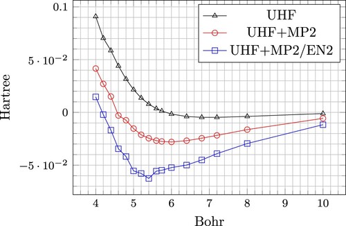
Table 5. Binding energy per atom for lithium in a bcc-structure as a function of the nearest-neighbour distance $r_{1\mathrm{N}\mathrm{N}}$.

$r_{1\mathrm{N}\mathrm{N}}$	UHF	PATMOS-MP2	PATMOS-EN2
(Bohr)	(Hartree)	(Hartree)	(Hartree)
4.0	0.090910	0.041582	0.014718
4.2	0.070408	0.027027	$-0.002089$
4.4	0.058668	0.015067	$-0.016804$
4.6	0.044060	$-0.002924$	$-0.034498$
4.8	0.031645	$-0.007449$	$-0.041831$
5.0	0.021540	$-0.015332$	$-0.055468$
5.2	0.013711	$-0.021193$	$-0.057872$
5.4	0.007857	$-0.024518$	$-0.062566$
5.6	0.003590	$-0.026755$	$-0.055675$
5.744214	0.001288	$-0.027535$	$-0.054842$
6.0	$-0.001570$	$-0.028011$	$-0.052314$
6.4	$-0.003881$	$-0.026800$	$-0.049904$
6.8	$-0.004666$	$-0.024473$	$-0.045075$
7.2	$-0.004695$	$-0.021769$	$-0.039113$
8.0	$-0.003810$	$-0.016312$	$-0.029502$
10.0	$-0.001093$	$-0.005653$	$-0.011636$

Notes: Basis set: $\left(11s1p/15s7p2d1f\right)$.

The character of the binding of solid lithium is disclosed in Table 6. To easily group the relative contribution of the components, we have used the magnitude of the Coulomb interaction as energy unit. The partitioning of the binding energy demonstrates very clearly that the correlation energy is of paramount importance. Its relative contribution increases with increasing value of $r_{1\mathrm{N}\mathrm{N}}$. There is one repulsive term: the distortion energy, i.e. the charge in intra-atomic energy due to the interaction with the surrounding atoms. The magnitude of the ‘semiclassical’ Coulomb energy, $E_{\mathrm{L}\mathrm{i};\mathrm{i}\mathrm{n}\mathrm{t}\mathrm{e}\mathrm{r}}^{\mathrm{C}\mathrm{o}\mathrm{u}\mathrm{l}}$, is less than the distortion energy for all distances considered in this work. As a consequence, the Hartree model, i.e. the UHF energy minus the exchange energy (UHF orbitals are used for the Hartree model) yield no binding. This feature is demonstrated in Table 7. Measured by the half-axes of the charge ellipsoid of the $2s$ orbital, we notice that there is only a small extension of the electron density at the experimental equilibrium distance $r_{1\mathrm{N}\mathrm{N}}=5.744214$ Bohr.

Table 6. Partitioning of the binding energy per atom, Equation (6(6) $E_A^{\mathrm{b}\mathrm{i}\mathrm{n}\mathrm{d}}={\mathrm{\Delta }}_A^{\mathrm{d}\mathrm{i}\mathrm{s}\mathrm{t}}+E_{A,\mathrm{i}\mathrm{n}\mathrm{t}\mathrm{e}\mathrm{r}}^{\mathrm{C}\mathrm{o}\mathrm{u}\mathrm{l}}+E_{A,\mathrm{i}\mathrm{n}\mathrm{t}\mathrm{e}\mathrm{r}}^{\mathrm{e}\mathrm{x}\mathrm{c}\mathrm{h}}+E_{A,\mathrm{i}\mathrm{n}\mathrm{t}\mathrm{e}\mathrm{r}}^{\mathrm{c}\mathrm{o}\mathrm{r}\mathrm{r}}$(6) ), for some nearest-neighbour distances.

$r_{1\mathrm{N}\mathrm{N}}$	${\mathrm{\Delta }}_{\mathrm{L}\mathrm{i}}^{\mathrm{d}\mathrm{i}\mathrm{s}\mathrm{t}}$	$E_{\mathrm{L}\mathrm{i};\mathrm{i}\mathrm{n}\mathrm{t}\mathrm{e}\mathrm{r}}^{\mathrm{C}\mathrm{o}\mathrm{u}\mathrm{l}}$	$E_{\mathrm{L}\mathrm{i};\mathrm{i}\mathrm{n}\mathrm{t}\mathrm{e}\mathrm{r}}^{\mathrm{e}\mathrm{x}\mathrm{c}\mathrm{h}}$	$E_{\mathrm{L}\mathrm{i};\mathrm{i}\mathrm{n}\mathrm{t}\mathrm{e}\mathrm{r}}^{\mathrm{c}\mathrm{o}\mathrm{r}\mathrm{r},\mathrm{M}\mathrm{P}2}$	$E_{\mathrm{L}\mathrm{i};\mathrm{i}\mathrm{n}\mathrm{t}\mathrm{e}\mathrm{r}}^{\mathrm{c}\mathrm{o}\mathrm{r}\mathrm{r},\mathrm{E}\mathrm{N}2}$	$E_{\mathrm{L}\mathrm{i}}^{\mathrm{b}\mathrm{i}\mathrm{n}\mathrm{d},\mathrm{E}\mathrm{N}2}$
(Bohr)	(Hartree)	(Hartree)	(Hartree)	(Hartree)	(Hartree)	(Hartree)
4.0	0.301008	$-0.134955$	$-0.075143$	$-0.049327$	$-0.076192$	0.014718
	(2.23)	($-1.00$)	($-0.56$)	($-0.37$)	($-0.56$)	(0.10)
5.0	0.132722	$-0.071144$	$-0.040038$	$-0.036874$	$-0.077010$	$-0.055468$
	(1.87)	($-1.00$)	($-0.56$)	($-0.52$)	($-1.08$)	($-0.78$)
5.4	0.098273	$-0.057901$	$-0.032515$	$-0.032374$	$-0.070422$	$-0.062566$
	(1.70)	($-1.00$)	($-0.56$)	($-0.56$)	($-1.22$)	($-1.08$)
5.744214	0.077579	$-0.049027$	$-0.027264$	$-0.028824$	$-0.056129$	$-0.054842$
	(1.58)	($-1.00$)	($-0.56$)	($-0.59$)	($-1.14$)	($-1.12$)
6.0	0.065675	$-0.043362$	$-0.023881$	$-0.026441$	$-0.050743$	$-0.052314$
	(1.51)	($-1.00$)	($-0.55$)	($-0.61$)	($-1.17$)	($-1.20$)
7.2	0.031712	$-0.023985$	$-0.012420$	$-0.017074$	$-0.034418$	$-0.039113$
	(1.32)	($-1.00$)	($-0.52$)	($-0.71$)	($-1.43$)	($-1.63$)
8.0	0.019544	$-0.015634$	$-0.007722$	$-0.012500$	$-0.025692$	$-0.029502$
	(1.25)	($-1.00$)	($-0.49$)	($-0.78$)	($-1.64$)	($-1.88$)
10.0	0.004235	$-0.003687$	$-0.001643$	$-0.004559$	$-0.010543$	$-0.011636$
	(1.15)	($-1.00$)	($-0.45$)	($-1.24$)	($-2.86$)	($-3.15$)

Notes: Values in parentheses are the magnitudes of the Coulomb interaction as energy unit. Basis set: $\left(11s1p/15s7p2d1f\right)$.

Table 7. Binding energy at the Hartree and UHF levels and the half-axes of the charge ellipsoid of the $2s$ orbital, as a function of the nearest-neighbour distance $r_{1\mathrm{N}\mathrm{N}}$.

$r_{1\mathrm{N}\mathrm{N}}$	Hartree model	UHF	$l_x=l_y=l_z$
(Bohr)	(Hartree)	(Hartree)	(Bohr)
4.0	0.166053	0.090910	2.037
5.0	0.061578	0.021540	2.353
5.4	0.040372	0.007857	2.398
5.744214	0.028552	0.001288	2.463
6.0	0.022313	$-0.001570$	2.504
7.2	0.007727	$-0.004695$	2.630
8.0	0.003950	$-0.003810$	2.663
10.0	0.000621	$-0.001093$	2.552

Notes: For isolated atom: $l_x=l_y=l_z=2.416$ Bohr. Basis set: $\left(11s1p/15s7p2d1f\right)$.

With exception of some round-off errors less than ${10}^{-6}$ Hartree, we have identical results for the α- and β-atoms of the reference unit cell. As for the inter-atomic interactions, those terms are only calculated for the α-type atom.

To summarise this section: binding of lithium in a bcc structure can be described by localised orbitals. The perturbed atomic orbitals are only slightly distorted. Furthermore, the correlation energy is extremely important in order to obtain an accurate binding enregy.

6. Discussion

There are mainly three different sources of error in this work: basis set, correlation energy and model errors. We consider first the basis set errors. At the distance $r_{1\mathrm{N}\mathrm{N}}=6.0$ Bohr, there is a small extension of the atomic electron density, see Table 7. The half-axes of the charge ellipsoid of the $2s$ orbital are respectively 2.504 Bohr and 2.498 Bohr for the two large basis sets $\left(15s7p2d1f\right)$ and $\left(19s8p7d5f2g1h\right)$. As demonstrated in Table 8, there are only small differences of the UHF energy components, roughly 1% or less. For the MP2 inter-atomic correlation energy the change is around 3%. Due to the unsystematic error of the EN2 component, the basis set effect is hidden in the unsystematic error. If we consider the difference between the two EN2 energies in Table 8 as a measure of the unsystematic error in the EN2 calculations, the error is roughly 7% of calculated correlation energy. This estimate is consistent with our previous one obtained in Section 5, i.e. 8%. In Table 9, the change in intra-atomic MP2 energy is shown as a function of the $r_{1\mathrm{N}\mathrm{N}}$ distance. The change is less than 1% for all distances considered. For the smaller large basis the change in intra-atomic MP2 energy due to the surrounding atoms, is 0.000060 Hartree to be compared with 0.000056 Hartree for the basis $\left(19s8p7d5f2g1h\right)$. Hence, the basis set error with respect to MP2 intra-atomic correlaton energy is negligible.

Table 8. Energy components of the binding energy per atom for two different large basis sets.

	${\mathrm{\Delta }}_{\mathrm{L}\mathrm{i}}^{\mathrm{d}\mathrm{i}\mathrm{s}\mathrm{t}}$	$E_{\mathrm{L}\mathrm{i};\mathrm{i}\mathrm{n}\mathrm{t}\mathrm{e}\mathrm{r}}^{\mathrm{C}\mathrm{o}\mathrm{u}\mathrm{l}}$	$E_{\mathrm{L}\mathrm{i};\mathrm{i}\mathrm{n}\mathrm{t}\mathrm{e}\mathrm{r}}^{\mathrm{e}\mathrm{x}\mathrm{c}\mathrm{h}}$	$E_{\mathrm{L}\mathrm{i};\mathrm{i}\mathrm{n}\mathrm{t}\mathrm{e}\mathrm{r}}^{\mathrm{M}\mathrm{P}2}$	$E_{\mathrm{L}\mathrm{i};\mathrm{i}\mathrm{n}\mathrm{t}\mathrm{e}\mathrm{r}}^{\mathrm{E}\mathrm{N}2}$
Basis	(Hartree)	(Hartree)	(Hartree)	(Hartree)	(Hartree)
$\left(11s1p/15s7p2d1f\right)$	0.065675	$-0.043362$	$-0.023881$	$-0.026441$	$-0.050743$
	(1.51)	($-1.00$)	($-0.55$)	($-0.61$)	($-1.17$)
$\left(11s1p/19s8p7d5f2g1h\right)$	0.065499	$-0.043205$	$-0.024105$	$-0.027095$	$-0.047194$
	(1.52)	($-1.00$)	($-0.56$)	($-0.63$)	($-1.09$)

Notes: Values in parentheses are the magnitudes of the Coulomb interaction as energy unit.

Table 9. The change in intra-atomic correlation energy as a function of the nearest-neighbour distance $r_{1\mathrm{N}\mathrm{N}}$.

$r_{1\mathrm{N}\mathrm{N}}$	$\mathrm{\Delta }{E}_{\mathrm{L}\mathrm{i};\mathrm{i}\mathrm{n}\mathrm{t}\mathrm{r}\mathrm{a}}^{\mathrm{M}\mathrm{P}2}$
(Bohr)	(Hartree)
4.0	$-0.000244$	$-0.7$%
5.0	$-0.000210$	$-0.6$%
6.0	0.000070	0.2%
7.2	0.000141	0.4%
8.0	0.000144	0.4%
10.0	0.000065	0.2%

Notes: For isolated Li: $E_{\mathrm{L}\mathrm{i};\mathrm{i}\mathrm{n}\mathrm{t}\mathrm{r}\mathrm{a}}^{\mathrm{M}\mathrm{P}2}=-0.035485$ Hartree. Basis set: $\left(11s1p/15s7p2d1f\right)$. $r_{1\mathrm{N}\mathrm{N}}=6.0$ Bohr.

There are two types of model errors in this work related to the spheres with distances $r_{\mathrm{m}\mathrm{o}\mathrm{d}\mathrm{e}\mathrm{l}}^{\mathrm{s}\mathrm{p}\mathrm{h}}$ and $r_{\mathrm{i}\mathrm{n}\mathrm{t}\mathrm{e}\mathrm{r}}^{\mathrm{s}\mathrm{p}\mathrm{h}}$, see Figure 2. The error of neglecting atoms outside the model sphere, i.e. the larger one, is well accounted for in this work. However, the interpair spheres with radius $r_{\mathrm{i}\mathrm{n}\mathrm{t}\mathrm{e}\mathrm{r}}^{\mathrm{s}\mathrm{p}\mathrm{h}}$ are the main sources of errors. In principle it can be reduced by increasing the radius $r_{\mathrm{i}\mathrm{n}\mathrm{t}\mathrm{e}\mathrm{r}}^{\mathrm{s}\mathrm{p}\mathrm{h}}$, say from $a_{\mathrm{u}\mathrm{c}}$ to $2a_{\mathrm{u}\mathrm{c}}$. But then the number of atoms in interpair spheres increases from 14 to 64, and the number of basis functions increases by almost a factor 5. Hence, at present this is not computationally feasible.

Our best estimate of the binding energy derived from a parabolic fit using the nearest-neighbour distances $\{5.0,5.2,5.6\}$ Bohr: $-0.05817$ Hartree. The binding energy per atom as a function of $r_{1\mathrm{N}\mathrm{N}}$, i.e. $E_{\mathrm{L}\mathrm{i}}^{\mathrm{b}\mathrm{i}\mathrm{n}\mathrm{d}}\left(r_{1\mathrm{N}\mathrm{N}}\right)$, is describing a collective contraction/expansion of the crystal. In approximating the nuclear motion of an atom, we use a harmonic potential. A straightforward calculation yields a zero-point vibratonal energy per atom equal to 0.00076 Hartree. With a 7% unsystematic error of EN2 correlation energy we arrive at the following estimate of the cohesive energy $0.0571\pm 0.004$ Hartree, comparing with experimental value[27] 0.0599 Hartree.

7. Concluding remarks

Our main objective of this work has been achieved: to construct a computationally feasible model for describing the electronic structure of pure metals using localised orbitals. Our calculated cohesive energy for lithium is in fair agreement with the experimental result.

A second point to emphasise is the importance of the electron correlation energy. The UHF model yields only a shallow minimum of the potential energy surface. Large basis sets are necessary conditions for obtaining reliable binding energies. A strong merit of the PATMOS model is the dual basis set approach. Large basis sets of the same quality as for molecules can be adopted. Furthermore, since we are using fixed atomic domains for the orbital spaces (slightly modified by orthogonality constraints), and we are calculating only diatomic corrections, linear dependencies can be avoided by just checking for linear dependency in calculations on the corresponding diatomic molecules.

A challenge for future work is to extend the model such that the unsystematic errors of the EN2 correlation energies can be reduced. Further, to improve the calculated correlation energy, we shall consider a more accurate model than EN2 for the nearest-neighbour atom pairs.

We are now in the beginning of a research programme devoted to the study of chemical binding using the PATMOS framework. As for solids, this implies time-consuming calculations. Some preliminary calculations on solid beryllium seem to indicate that bonding in this case might not be correlation driven. The results will be reported in due time.

Finally, if our conjecture concerning localised orbitals and bonding in metals, can be confirmed, then there is nice similarity between molecules and metals: bonding for both types of systems is most appropriately described by localised orbitals, but for spectroscopy canonical orbitals is the proper choice.

Disclosure statement

No potential conflict of interest was reported by the author(s).

Additional information

Funding

This work was supported by the Research Council of Norway (Norges forskningsråd) through its Centres of Excellence scheme [project number 262695]. This work has received support from the Norwegian Supercomputer Program (NOTUR) through a grant of computer time [grant number NN4654K].

Appendix

Symmetric orthonormalization of spin orbitals

Let A denote an atom in the reference unit cell, and $A_p$ an atom of the same type in the BF-region of atom A. The number of atoms of type A, excluding atom A, in the BF-region of A is denoted $N_A^{\mathrm{p}\mathrm{a}\mathrm{r}\mathrm{t}\mathrm{n}\mathrm{e}\mathrm{r}}$. The set of partner atoms in the BF-region: (A1) ${\mathrm{\Omega }}_{\mathrm{B}\mathrm{F}}^{A,\mathrm{p}\mathrm{a}\mathrm{r}\mathrm{t}\mathrm{n}\mathrm{e}\mathrm{r}}=\{A_p;1\le p\le N_A^{\mathrm{p}\mathrm{a}\mathrm{r}\mathrm{t}\mathrm{n}\mathrm{e}\mathrm{r}}\}.$(A1) For a fixed modified one-centre basis $\{{\tilde{\chi }}_{\mu }^{A_p,\mathrm{l}\mathrm{b};\alpha };1\le \mu \le m_A^{\mathrm{l}\mathrm{b}}\}$, we construct an iterative procedure for symmetrising the α-type orbitals: $\{{\psi }_i^{A,\alpha };1\le i\le N_A^{\alpha }\}\stackrel{N_A^{\mathrm{p}\mathrm{a}\mathrm{r}\mathrm{t}\mathrm{n}\mathrm{e}\mathrm{r}}}{\underset{p=1}{\cup }}\{{\psi }_i^{A_p,\alpha };1\le i\le N_A^{\alpha }\}$.

For each atom pair $(A,A_p)$ we perform a symmetric orthonormalization of the set, $\{{\psi }_i^{A,\alpha };1\le i\le N_A^{\alpha }\}\stackrel{N_A^{\mathrm{p}\mathrm{a}\mathrm{r}\mathrm{t}\mathrm{n}\mathrm{e}\mathrm{r}}}{\underset{p=1}{\cup }}\{{\psi }_i^{A_p,\alpha };1\le i\le N_A^{\alpha }\}$. As a result we obtain $\{{\hat{\psi }}_i^{A,\alpha };1\le i\le N_A^{\alpha }\}$. Then we project this set onto $\{{\tilde{\chi }}_{\mu }^{A_p,\mathrm{l}\mathrm{b};\alpha };1\le \mu \le m_A^{\mathrm{l}\mathrm{b}}\}$. A symmetric orthonormalization of the prjected orbitals yields $\left\{{\tilde{\psi }}_i^{A,\alpha }\right(A_p);1\le i\le N_A^{\alpha }\}$. The argument $A_p$ in the orbital symbol emphasises that the modification of the orbitals is due to the orbtials of atom $A_p$. An orbital correction is given by the equation (A2) $\mathrm{\Delta }{\tilde{\psi }}_i^{A,\alpha }\left(A_p\right)={\tilde{\psi }}_i^{A,\alpha }\left(A_p\right)-{\psi }_i^{A,\alpha },$(A2) and accumulated correction is (A3) $\mathrm{\Delta }{\psi }_i^{A,\alpha }=\sum _{p=1}^{N_A^{\mathrm{p}\mathrm{a}\mathrm{r}\mathrm{t}\mathrm{n}\mathrm{e}\mathrm{r}}}\mathrm{\Delta }{\tilde{\psi }}_i^{A,\alpha }\left(A_p\right).$(A3) A new set of orbitals for atom A is defined as (A4) ${\tilde{\psi }}_i^{A,\alpha }={\psi }_i^{A,\alpha }+\mathrm{\Delta }{\psi }_i^{A,\alpha },1\le i\le N_A^{\alpha }.$(A4) Symmetric orthonormalization of $\{{\tilde{\psi }}_i^{A,\alpha };1\le i\le N_A^{\alpha }\}$ yields $\{{\psi }_i^{\mathrm{s}\mathrm{y}\mathrm{m};A,\alpha };1\le i\le N_A^{\alpha }\}$. The iterative cycle is then repeated. Typically, 15–20 cycles are required in order to have a converged result. If the procedure does not converge within a fixed number of cycles, the parameter λ in Equation (35(35) $\begin{array}{rl}{\psi }_i^A\left(\lambda \right)& ={\psi }_i^{A,\mathrm{o}\mathrm{l}\mathrm{d}}+\lambda ({\psi }_i^{A,\mathrm{n}\mathrm{e}\mathrm{w}}-{\psi }_i^{A,\mathrm{o}\mathrm{l}\mathrm{d}}),\\ & 1\le A\le N_{\mathrm{a}\mathrm{t}\mathrm{o}\mathrm{m}\mathrm{s}}^{\mathrm{u}\mathrm{c}},1\le i\le N_A,0<\lambda \le 1.\end{array}$(35) ), i.e. the step length, is reduced.

References

- G.N. Lewis, J. Am. Chem. Soc. 38 (4), 762–785 (1916). doi:10.1021/ja02261a002
- K. Ruedenberg, Rev. Mod. Phys. 34, 326–376 (1962). doi:10.1103/RevModPhys.34.326
- G. Frenking and S. Shaik, The Chemical Bond: Fundamental Aspects of Chemical Bonding (John Wiley & Sons, Ltd., Weinheim, 2014).
- I. Røeggen and B. Gao, J. Chem. Phys. 139 (9), 094104 (2013). doi:10.1063/1.4818577
- I. Røeggen and B. Gao, J. Chem. Phys. 148 (13), 134118 (2018). doi:10.1063/1.5018148
- P. Pulay, Chem. Phys. Lett. 100 (2), 151–154 (1983). doi:10.1016/0009-2614(83)80703-9
- S. Sæbø and P. Pulay, Chem. Phys. Lett. 113 (1), 13–18 (1985). doi:10.1016/0009-2614(85)85003-X
- S. Sæbø and P. Pulay, J. Chem. Phys. 86 (2), 914–922 (1987). doi:10.1063/1.452293
- S. Sæbø and P. Pulay, J. Chem. Phys. 88 (3), 1884–1890 (1988). doi:10.1063/1.454111
- D. Usvyat, L. Maschio and M. Schütz, WIREs Comput. Mol. Sci. 8 (4), e1357 (2018). doi: 10.1002/wcms.1357.
- E. Rebolini, G. Baardsen, A.S. Hansen, K.R. Leikanger and T.B. Pedersen, J. Chem. Theory Comput.14 (5), 2427–2438 (2018). doi:10.1021/acs.jctc.8b00021
- Y. Wang, Z. Ni, W. Li and S. Li, J. Chem. Theory Comput. 15 (5), 2933–2943 (2019). doi:10.1021/acs.jctc.8b01200
- R.K. Nesbet, Adv. Chem. Phys. 14, 1 (1969). doi:10.1002/9780470143599.ch1.
- H. Stoll, Phys. Rev. B 46 (11), 6700–6704 (1992). doi:10.1103/PhysRevB.46.6700
- H. Stoll, J. Chem. Phys. 97 (11), 8449–8454 (1992). doi:10.1063/1.463415
- A. Shukla, M. Dolg, P. Fulde and H. Stoll, Phys. Rev. B 57 (3), 1471–1483 (1998). doi:10.1103/PhysRevB.57.1471
- I. Røeggen, J. Chem. Phys. 79 (11), 5520–5531 (1983). doi:10.1063/1.445670
- I. Røeggen, in Correlation and Localization, edited by P.R. Surján, Topics in Current Chemistry, Vol. 203 (Springer, Berlin, 1999), pp. 89–103.
- L. Bytautas and K. Ruedenberg, J. Phys. Chem. A 114 (33), 8601–8612 (2010). doi:10.1021/jp9120595
- E. Voloshina and B. Paulus, J. Chem. Theory Comput. 10 (4), 1698–1706 (2014). doi:10.1021/ct401040t
- B. Paulus and H. Stoll, in Accurate Condensed-Phase Quantum Chemistry, edited by F. Manby, 1st ed., Chap. 3, Computation in Chemistry (CRC Press, Boca Raton, 2011), pp. 57–84.
- M.A. Robb, W.J. Haines and I.G. Csizmadia, J. Am. Chem. Soc. 95 (1), 42–48 (1973). doi:10.1021/ja00782a007
- N.H.F. Beebe and J. Linderberg, Int. J. Quantum Chem. 12 (4), 683–705 (1977). doi:10.1002/(ISSN)1097-461X
- I. Røeggen and E. Wisløff-Nilssen, Chem. Phys. Lett. 132 (2), 154–160 (1986). doi:10.1016/0009-2614(86)80099-9
- H. Koch, A. Sánchez de Merás and T.B. Pedersen, J. Chem. Phys. 118 (21), 9481–9484 (2003). doi:10.1063/1.1578621
- I. Røeggen and T. Johansen, J. Chem. Phys. 128 (19), 194107 (2008). doi:10.1063/1.2925269
- C. Kittel, Introduction to Solid State Physics, 5th ed. (John Wiley & Sons, New York, 1976).
- J. Emsley, The Elements (Oxford University Press, Oxford, 1994).