Vibrational, non-adiabatic and isotopic effects in the dynamics of the H₂ + H₂⁺ → H₃⁺ + H reaction: application to plasma modelling

Abstract

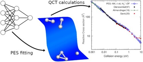
The title reaction is studied using a quasi-classical trajectory method for collision energies between 0.1 meV and 10 eV, considering the vibrational excitation of ${\mathrm{H}}_2^{+}$ reactant. A new potential energy surface is developed based on a Neural Network many body correction of a triatomics-in-molecules potential, which significantly improves the accuracy of the potential up to energies of 17 eV, higher than in other previous fits. The effect of the fit accuracy and the non-adiabatic transitions on the dynamics are analysed in detail. The reaction cross section for collision energies above 1 eV increases significantly with the increasing of the vibrational excitation of ${\mathrm{H}}_2^{+}$($v^{\mathrm{\prime }}$), for values up to $v^{\mathrm{\prime }}$=6. The total reaction cross section (including the double fragmentation channel) obtained for $v^{\mathrm{\prime }}$=6 matches the new experimental results obtained by Savic, Schlemmer and Gerlich [Chem. Phys. Chem. 21 (13), 1429.1435 (2020). doi:10.1002/cphc.v21.13]. The differences among several experimental setups, for collision energies above 1 eV, showing cross sections scattered/dispersed over a rather wide interval, can be explained by the differences in the vibrational excitations obtained in the formation of ${\mathrm{H}}_2^{+}$ reactants. On the contrary, for collision energies below 1 eV, the cross section is determined by the long range behaviour of the potential and do not depend strongly on the vibrational state of ${\mathrm{H}}_2^{+}$. In addition in this study, the calculated reaction cross sections are used in a plasma model and compared with previous results. We conclude that the efficiency of the formation of ${\mathrm{H}}_3^{+}$ in the plasma is affected by the potential energy surface used.

GRAPHICAL ABSTRACT

Keywords:

• Potential energy surfaces
• non-adiabatic dynamics
• isotopic and vibrational effects
• plasmas
• astrochemistry

1. Introduction

Hydrogen, as the most abundant element in the Universe, plays a fundamental role in star formation and the chemical evolution of molecular Universe. Its molecular forms are ${\mathrm{H}}_2$, ${\mathrm{H}}_2^{+}$ and ${\mathrm{H}}_3^{+}$ [1]. In evolved galaxies, the formation of ${\mathrm{H}}_2$ is usually attributed to atomic hydrogen recombination on cosmic grains and ices [2–4]. ${\mathrm{H}}_2^{+}$ is rapidly formed by cosmic rays or electrons, and it collides with ${\mathrm{H}}_2$ to form ${\mathrm{H}}_3^{+}$ in the reaction (1) ${\mathrm{H}}_2(v,j)+{\mathrm{H}}_2^{+}(v^{\mathrm{\prime }},j^{\mathrm{\prime }})\to {\mathrm{H}}_3^{+}+\mathrm{H}.$(1) Once the molecular forms of hydrogen are formed, the chemistry in space starts with the formation of the first hydrides. In cold clouds, the most abundant ion is ${\mathrm{H}}_3^{+}$, which is considered to be the universal protonator [5–8] through the proton hop reaction [1, 9] (2) ${\mathrm{H}}_3^{+}+\mathrm{M}\to {\mathrm{HM}}^{+}+{\mathrm{H}}_2,$(2) where M is an atom or a molecule. The HM${}^{+}$ cations are very reactive and trigger many chemical networks giving rise to most of the molecular systems detected in space [5–8, 10, 11]. In cold environments, M colliders in Equation (2(2) ${\mathrm{H}}_3^{+}+\mathrm{M}\to {\mathrm{HM}}^{+}+{\mathrm{H}}_2,$(2) ) deposit on ices, and ${\mathrm{H}}_3^{+}$ reacts only with the most abundant molecule, ${\mathrm{H}}_2$, as (3) ${\mathrm{H}}_2+{\mathrm{H}}_3^{+}\to {\mathrm{H}}_3^{+}+{\mathrm{H}}_2,$(3) a proton exchange reaction, which is constrained by nuclear spin statistic [12–18], and is the responsible for the ortho/para ratio of ${\mathrm{H}}_3^{+}$. When the collider is HD, reaction (3(3) ${\mathrm{H}}_2+{\mathrm{H}}_3^{+}\to {\mathrm{H}}_3^{+}+{\mathrm{H}}_2,$(3) ) is the responsible of ${\mathrm{H}}_3^{+}$ deuteration [13, 17, 19–24]. The deuterated species formed following Equation (2(2) ${\mathrm{H}}_3^{+}+\mathrm{M}\to {\mathrm{HM}}^{+}+{\mathrm{H}}_2,$(2) ) produce the observed high relative abundance of deuterated species, estimated as ≈ 10${}^4$ times higher than the D/H ratio of the galaxy [25–28]. This high deuteration efficiency is attributed to the zero-point energy differences among the ${\mathrm{H}}_3^{+}$ deuterated species, very significant at the low temperatures of cold molecular clouds [22, 29].

Hydrogen plasma [30–32], apart from their technological applications in industry, medicine and fusion reactors [33, 34], can be considered as a prototype for Early Universe models [2, 35–38]. In the absence of other species but hydrogen, the molecular species are simply ${\mathrm{H}}_2$, ${\mathrm{H}}_2^{+}$ and ${\mathrm{H}}_3^{+}$, but ${\mathrm{H}}^{+}$ also exists. The distribution of the ions affects the determination of hydrogen particle flux in the plasma [39, 40]. The reaction in Equation (1(1) ${\mathrm{H}}_2(v,j)+{\mathrm{H}}_2^{+}(v^{\mathrm{\prime }},j^{\mathrm{\prime }})\to {\mathrm{H}}_3^{+}+\mathrm{H}.$(1) ) is an important process for modelling ${\mathrm{H}}_2$ plasma at low electron and molecular temperatures ($T_e\sim 5$ eV, $T_m\sim 0.1$ eV) since the process is the only dominant process for the formation of ${\mathrm{H}}_3^{+}$ [41]. Therefore, an accurate cross section is essential for the determination of the density of ${\mathrm{H}}_3^{+}$ in plasma models. Moreover, the rovibrationally resolved cross sections are required for collisional-radiative (CR) spectroscopic modelling of molecular hydrogen which can be applied to a fusion detached plasma [42, 43]. The isotopic effect on the reaction is also essential for plasma modelling in nuclear fusion tokamak [44].

The reaction in Equation (1(1) ${\mathrm{H}}_2(v,j)+{\mathrm{H}}_2^{+}(v^{\mathrm{\prime }},j^{\mathrm{\prime }})\to {\mathrm{H}}_3^{+}+\mathrm{H}.$(1) ) has been widely studied experimentally [45–54] and theoretically [49, 55–60]. In the 1 meV and 1 eV energy interval, an excellent agreement between experimental [54] and theoretical [60] reactive cross sections has been achieved. Recently, this reaction has been studied in two extreme regimes, at ultra cold energies [61–64] and at high collision energies [65] up to 10 eV. At ultra cold energies, many isotopic variants have been studied, and the reactive cross section shows a Langevin-like behaviour so that the measured reactive cross sections, in relative units, shows also excellent agreement with the theoretical simulations [60]. However, recent experiments performed at higher collision energies (1-10 eV) [65] differ considerably from previous theoretical simulations [49, 55, 60]. Moreover, for collision energies above 1 eV, the new experimental measurements show differences with previous experimental ones [45–48, 52, 53], all of them scattered in a rather wide interval of cross sections.

There are two main goals in this work. First, we focus on the theoretical simulations of the ${\mathrm{H}}_3^{+}$ formation reaction, Equation (1(1) ${\mathrm{H}}_2(v,j)+{\mathrm{H}}_2^{+}(v^{\mathrm{\prime }},j^{\mathrm{\prime }})\to {\mathrm{H}}_3^{+}+\mathrm{H}.$(1) ), to reproduce the new experimental data above 1 eV [65]. Second, we study hydrogen or deuterium plasma models in order to analyse the effects of the calculated cross sections and rates on the ${\mathrm{H}}_3^{+}$ or D${}_3^{+}$ densities.

This work is organised as follows. In Section 2, we develop new potential energy surfaces (PESs), which include non-adiabatic effects and increase the accuracy of the fit. This new fit uses a Neural Network (NN) method to describe the four-body term, to improve a zero-order description using a Triatomics-in-Molecule treatment, which accurately fits very precise ab initio calculations, over a broader energy interval than previous fits, up to 17 eV. In Section 3, we study the reaction dynamics using a quasi-classical trajectory (QCT) method, including transitions among different electronic states, using the fewest switches method of Tully [66]. The reaction dynamics is studied for collision energies between 1 meV and 10 eV, and for several vibrational states of ${\mathrm{H}}_2^{+}$ reactant, as well as for the deuterated reaction, focussing on high energy reactive cross sections recently measured by Savic et al. [65]. In Section 4, we investigate how the calculated reactive cross sections affect the population density of ${\mathrm{H}}_3^{+}$ and D${}_3^{+}$ in CR models of ${\mathrm{H}}_2$/D${}_2$ plasma. Finally, in Section 5 some conclusions are extracted.

2. Potential energy surfaces of ${\mathrm{H}}_4^{+}$

In this work several PESs are used, and are listed here to clarify the differences:

PES1:	This PES developed by Sanz-Sanz et al. [67], is the most accurate developed so far for this system. It is built as a sum of a triatomics-in-molecules (TRIM) term, $H^{\mathrm{TRIM}}$, plus a four body term, $H^{\mathrm{MB}}$. The TRIM term is a generalisation of the Diatomics-in-Molecules (DIM) [68–71] method, in which the electronic Hamiltonian is factorised as a sum of triatomic and diatomic fragments as [67, 72] (4) ${\hat{H}}_e^i=\sum _{n>i,o>n}{\hat{H}}_{\mathrm{ino}}^{+}(n-i,o-i)-\sum _{p>i}{\hat{H}}_{\mathrm{ip}}^{+}(p-i)$(4) where ${\hat{H}}_{\mathrm{ip}}^{+}$ are the monoelectronic Hamiltonians of ${\mathrm{H}}_2^{+}$ fragments and ${\hat{H}}_{\mathrm{ino}}^{+}(n-i,o-i)$ are the bielectronic Hamiltonians (for n−i, o−i electrons) describing the ${\mathrm{H}}_3^{+}$ system for the ino nuclei. The TRIM representation consists of a 8×8 matrix, whose elements have ${\mathrm{H}}_3^{+}$ and ${\mathrm{H}}_2^{+}$ matrix elements of different electronic configurations, in which each hydrogen atom is described by a 1s function, except one corresponding to ${\mathrm{H}}^{+}$. In PES1 [67], the triatomic terms included in the TRIM matrix were built as the 3×3 DIM matrix for each ${\mathrm{H}}_3^{+}$ fragment plus a three-body term added to describe the ground state of either singlet or triplet symmetry. The non-adiabatic terms in these triatomic fragments are therefore approximated by those obtained in a DIM treatment. PES1 is built adding a four-body correction (MB term) to this TRIM description. This MB term is expressed as a linear combination of four-body polynomials that are symmetric with respect to the permutations of identical nuclei (Permutationally invariant polynomials or PIP). These PIP are built in terms of Rydberg polynomials of the interatomic distances ($p_i=r_i\exp (-{\alpha }_i{r}_i)$) [73–75]. The set of linear and non linear coefficients, ${\alpha }_i$, are optimised to minimise the difference with the ab initio energies obtained with the multi reference configuration interaction (MRCI) method using the aug-cc-pV5Z basis set [76]. In PES1, the same four-body correction term is added to all the diagonal elements of the TRIM matrix. The reactive cross sections calculated on this PES1 shows an excellent agreement with the experimental results for collision energies between 1 meV and 1 eV [60–62, 65].
PESTRIM8×8 and PESTRIM1×1:	This PES is based on the TRIM model explained above, and is an improvement made in this work. The main difference is that the triatomic ${\mathrm{H}}_3^{+}$ is represented by 3×3 diabatic matrices fitting its three lowest singlet and triplet electronic states [77] to MRCI ab initio energies extrapolated to the complete basis set (CBS) limit [78]. This improvement is crucial to study the non-adiabatic dynamics of ${\mathrm{H}}_4^{+}$. Analytical derivatives of the potential energy surfaces and non-adiabatic couplings are calculated based on the Hellmann-Feynmann theorem as described in [60]. The full PESTRIM8×8 potential correspond to the eight adiabatic eigenvalues including the non-adiabatic coupling terms. PESTRIM1×1 only considers the ground adiabatic energy.
PES-NN:	PESTRIM1×1 lacks high accuracy in the interaction region, i.e. where ${\mathrm{H}}_4^{+}$ is formed, while showing excellent agreement for ${\mathrm{H}}_3^{+}+\mathrm{H}$ or ${\mathrm{H}}_2$ + ${\mathrm{H}}_2^{+}$ rearrangement channels. For this reason a four-body neural network term is added to PESTRIM1×1 to improve the accuracy of the system, as described below.

2.1. Many body neural network term

Many body potential energy terms are widely used to represent potential energy surface of chemical systems, either in a many body expansion [74, 79, 80], where one up to N-body terms are summed, or as correction terms of a zero-order description of the potential, described by the TRIM method [67, 72] or by a reactive force field matrix [81–83].

In this work a many body neural network (MB-NN) [83] potential energy term has been built as a PIP-NN [84], in which the neural network is fed with a permutational invariant polynomial representation of the molecular geometry. A PIP is constructed by projecting a polynomial of the interatomic distances into the totally symmetric irreducible representation of the desired permutation group. A generator of these PIPs is defined as: (5) $P_n=\hat{S}\prod _{i=1}^{N_d}{p}_i^{l_i^n}\left(r_i\right)$(5) where $N_d$ is the number of interatomic distances, $p_i$ is a function of the interatomic distance $r_i$, $l_i^n$ is the exponent of the ith monomial for the nth polynomial and $\hat{S}$ is the projector to the totally symmetric irreducible representation of the permutation group. A common choice of $p\left(r\right)$ in PIP-NN-PES is the decaying exponential $p_i\left(r\right)=\exp (-{\alpha }_{i}r)$.

The set of PIP has to be carefully filtered so that it is purely composed of N-body functions. This means that any of these functions evaluated on a geometry where the N bodies are not closely interacting should be zero. In case these terms included any lower body functions, we have shown that it would add spurious interactions between fragments [85], which specially affects the long range regions.

In Appendix A it is shown that a polynomial in Equation (5(5) $P_n=\hat{S}\prod _{i=1}^{N_d}{p}_i^{l_i^n}\left(r_i\right)$(5) ) can be represented as a graph, and that the subset of N-body polynomials corresponds to those whose respective graph is connected, meaning that there exists a path which connects all the vertices (particles) of the graph. In this way we can guarantee that any N-body polynomial, with $p\left(r\right)$ defined as a decaying exponential or Rydberg function, will tend to zero as any particle or set of particles moves away from the rest. This will automatically make zero a PIP-PES and provide constant descriptor for a NN-PIP-PES, that returns a constant energy out of the N-body region, which can be trained to be as close to zero as possible and that produces no net force, since its derivative with respect to the atom coordinates is zero.

The four-body term developed here is expressed as a feed forward neural net with 11 input neurons and two hidden layers with $N_2$ = 32 and $N_3$ = 77, and sigmoid non linearities $\sigma =1/(1+\exp (-x\left)\right)$: (6) $\begin{array}{rl}{H}^{\mathrm{MB}}& =b_1^{\left(3\right)}+\sum _i^{N_3}(w_{1i}^{\left(3\right)}\sigma (b_i^{\left(2\right)}+\sum _j^{N_2}(w_{\mathrm{ij}}^{\left(2\right)}\sigma (\phantom{\sum _k^{N_1}}{b}_k^{\left(1\right)}\\ & +\sum _k^{N_1}\left(w_{\mathrm{jk}}^{\left(1\right)}\mathrm{PI}{P}_k\right)))\phantom{\sum _j^{N_2}}))\end{array}$(6) were ${\mathbf{w}}^{\left(l\right)}$ matrix (with elements $w_{\mathrm{ki}}^{\left(l\right)}$) and ${\mathbf{b}}^{\left(l\right)}$ vector (with elements $b_i^{\left(l\right)}$) represent the trainable weights and bias on layer l. The 11 input neurons correspond to four-body PIPs produced by setting a maximum polynomial degree max($\sum l_i$) = 5 and maximum monomial degree max($l_i$)=2. All lower body polynomials that would introduce spurious energy contributions in reactants and products channels are filtered following the steps detailed in Appendix A.

The four-body term is trained with NeuralPES, an in-house Python code based on PyTorch [86]. New ab initio points have been used in the fit of this work, of higher accuracy of those used in PES1 [67]. The energies are obtained using a two point extrapolation method to complete basis set (CBS) [78], using the results obtained with the aug-cc-pV5Z and aug-cc-pV6Z basis sets. Around 33000 ab initio points were calculated, including the geometries of Ref. [67] and new ones selected to increase the accuracy of the PES above 2 eV. These last new points were chosen from QCT trajectories at different collision energies (from 1 eV to 10 eV) taken on the TRIMPES1×1 to populate physically accessible configurations at this high energy regions. The complete set of ab initio points is randomly split into a training set (containing 80% of the data) and validation and test sets (with 10% of the points each). The training set consists on 27294 geometries, with energies up to 17 eV over the ${\mathrm{H}}_2$ + ${\mathrm{H}}_2^{+}$ asymptote, mostly corresponding to four-body interactions, and elongations to lower body geometries. The training process aims to minimise the root mean squared error between the ab initio and PESTRIM1×1 + $H^{\mathrm{MB}}$ energies.

2.2. Analysis of the different PESs

As all the four-body terms described above vanish as the systems tend to reactants or product asymptotes, the long-range interactions are purely described by the triatomic terms of the TRIM model. In all the triatomic fits considered here, the long range terms for ${\mathrm{H}}_2$ + ${\mathrm{H}}^{+}$ and ${\mathrm{H}}_2^{+}+\mathrm{H}$ fragments, for either singlet or triplet states are very precisely described [77, 87, 88]. This produces highly accurate long-range interaction in the ${\mathrm{H}}_2$ + ${\mathrm{H}}_2^{+}$ channel [60]. Allmendinger et al. [61, 62] applied a new experimental set up to study ${\mathrm{H}}_2^{+}$ + ${\mathrm{H}}_2$ $\to$ ${\mathrm{H}}_3^{+}+\mathrm{H}$ reaction at low temperatures. The measured cross section was then scaled to reproduce the cross section calculated with the PES1 potential [60] at a single collision energy. The excellent agreement between calculated and scaled experimental cross sections between 0.5 and 5 meV demonstrates the good behaviour of the long-range interactions included in PES1. The new PESs introduced in this work, describes the long-range interaction even more accurately, by using improved long-range interactions in the triatomic fragments [77]. The RMS errors for the different potential energy surfaces are presented in Table 1, in different energy intervals. The improvement of PES-NN over PESTRIM1×1 is clear in all energy ranges due to the enhancement of the ${\mathrm{H}}_4^{+}$ channels as presented in Table 2. PES1 and PES-NN show comparable RMSE for energies below 2 eV, but when ab initio points above 2 eV are added, PES-NN shows a much higher accuracy.

The whole configuration space is divided as follows: when all the interatomic distances are below $R_{\mathrm{thres}}=4$ Å, the system is taken to be in ${\mathrm{H}}_4^{+}$ region; if all interatomic distances of a triad of hydrogens are shorter than $R_{\mathrm{thres}}$, the region is taken to be ${\mathrm{H}}_3^{+}+\mathrm{H}$; if any two pairs of atoms present interatomic distances shorter than $R_{\mathrm{thres}}$, the region is denoted as ${\mathrm{H}}_2$ + ${\mathrm{H}}_2^{+}$; if only one internuclear distance is $<R_{\mathrm{thres}}$, the region is called ${\mathrm{H}}_2+\mathrm{H}+{\mathrm{H}}^{+}$; otherwise, if all the interatomic distances are large, the system is in fully dissociated. Following this division, the top left panel of Figure 1 shows the distribution of the data set among the different regions as defined above, as a function of the energy, taking the ${\mathrm{H}}_2$ + ${\mathrm{H}}_2^{+}$ reactants asymptote as the zero of energy. Most of the data correspond to ${\mathrm{H}}_4^{+}$ and geometries which connect this channel to ${\mathrm{H}}_2$ + ${\mathrm{H}}_2^{+}$ and ${\mathrm{H}}_3^{+}+\mathrm{H}$. As can be seen in the top right and bottom panels, the PESTRIM1×1 is highly accurate in the latter two channels, but shows deviations in the ${\mathrm{H}}_4^{+}$ region, up to several eV. The effect of the four-body term on PES-NN is decisive for the proper description of ${\mathrm{H}}_4^{+}$ region. PES1 was fitted for energies up to ≈ 2 eV, and it presents large energy deviations over this threshold. On the contrary, PES-NN keeps a high precision at high energies, which are the interest of the present work.

Figure 1. The top left panel shows the energy distribution of training data in three regions of the configuration space, as described in the text. Top right and bottom panels show the energy difference between the three PES considered in this work and ab initio calculations.

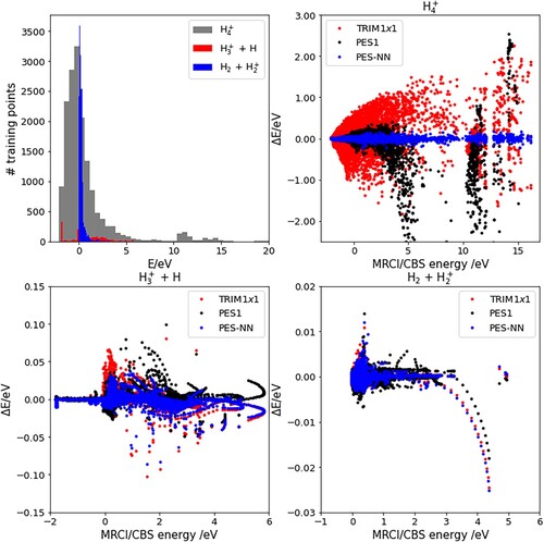
Table 1. Root mean squared errors of the ground electronic state for different energy regions, defined for $E<E_c$.

E${}_c$ (eV)	Points	PES1 (meV)	PESTRIM1×1 (meV)	PES-NN (meV)
0.0	9314	16.27	145.49	10.02
2.5	30856	25.08	131.21	10.41
5.0	32314	98.58	151.64	11.65
7.5	32544	334.96	161.20	12.15
10.0	32622	850.30	164.88	12.37
12.5	33007	1390.21	170.04	12.77
15.0	33189	2041.10	183.78	13.24

Notes: The number of points on which the RMSE is calculated is presented. The zero of energy is set at ${\mathrm{H}}_2$ + ${\mathrm{H}}_2^{+}$ asymptote, with the two fragment in their equilibrium configuration.

Table 2. Root mean squared errors of the ground electronic state for different channels, calculated on all the geometries with energy lower than 17 eV.

Region	Points	PES1 (meV)	PESTRIM1×1 (meV)	PES-NN (meV)
${\mathrm{H}}_4^{+}$	16034	3451.60	270.27	18.97
${\mathrm{H}}_3^{+}+\mathrm{H}$	3096	9.81	12.69	8.99
${\mathrm{H}}_2$ + ${\mathrm{H}}_2^{+}$	14031	0.87	0.74	0.82

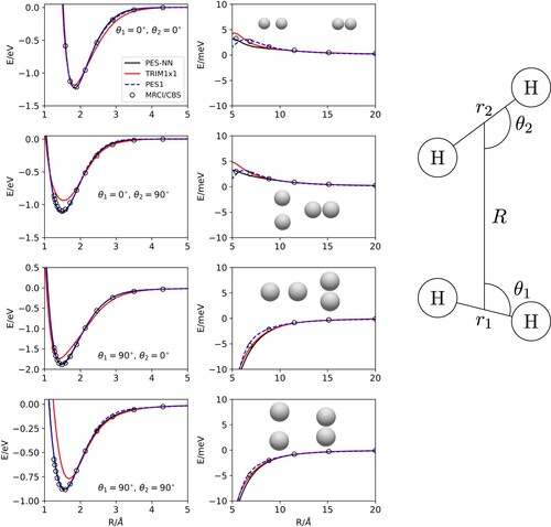
In Figure 2, ${\mathrm{H}}_2$ + ${\mathrm{H}}_2^{+}$ approaches for different ${\theta }_1$ and ${\theta }_2$ angles in their equilibrium geometry are shown for the three potential energy surfaces and compared with ab initio calculations. PESTRIM1×1 tends to predict a larger energy for ${\mathrm{H}}_4^{+}$ geometries, while PES1 and PES-NN yield effectively the same description. As the interfragment distance increases towards ${\mathrm{H}}_2$ + ${\mathrm{H}}_2^{+}$ the four-body terms in both PES1 and PES-NN go to zero and all that remains are the respective TRIM terms. The improvement of the new PES-NN is better seen when the diatomic fragments are not at the equilibrium geometry, for energies above 2 eV.

Figure 2. ${\mathrm{H}}_2$ + ${\mathrm{H}}_2^{+}$ approaches for several ${\theta }_1$ and ${\theta }_2$ angles and $r_1=0.740$ Å (for ${\mathrm{H}}_2$) and $r_2=1.055$ Å (for ${\mathrm{H}}_2^{+}$) the equilibrium distances of both species. The inset in the right hand side shows the coordinates used.

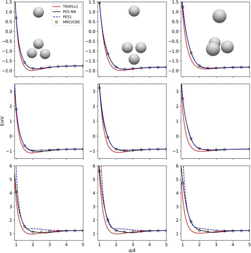
The more accurate description of the higher energy regime, energies larger than 2 eV, can be seen in Figure 3 where H approaches to a compressed ${\mathrm{H}}_3^{+}$. The differences between PES1 and PES-NN are more pronounced when bonds are compressed than stretched. This is

Figure 3. ${\mathrm{H}}_3^{+}+\mathrm{H}$ approaches, as a function of d, the distance of H to the ${\mathrm{H}}_3^{+}$ centre-of-mass. The orientations are preserved in the columns. The rows correspond to different equilateral ${\mathrm{H}}_3^{+}$ bond distances: top panels 0.85Å (equilibrium), middle panels to 0.7 Å and bottom panels to 0.6 Å, respectively. In the top panel, corresponding to ${\mathrm{H}}_3^{+}$ equilibrium configuration, the asymptotic energy is -1.816 eV.

3. Reaction dynamics

3.1. Quasi-classical trajectory and surface hoping calculations

The quasi-classical trajectory calculations are performed with the MDwQT code [60, 82, 89, 90]. When considering several coupled adiabatic electronic states, the fewest switches approach of Tully [66] is used as described in [60]. Initial conditions are sampled with the usual Monte Carlo method [91]. The initial conditions for the vibrational modes of ${\mathrm{H}}_2$ and ${\mathrm{H}}_2^{+}$ are quantised using the adiabatic switching method [92–94], yielding vibrational energies within 0.3 meV with respect to the exact vibrational levels of each diatomic fragment. The rotational states of ${\mathrm{H}}_2$ and ${\mathrm{H}}_2^{+}$ are set to zero in these studies, and the initial distance between the two centre-of-mass is set to 105 bohr. The initial impact parameter, b, is sampled between 0 and B, according to a quadratic distribution on b, where B is determined for each energy according to a capture model [95] as $B=(\alpha /2E{)}^{1/4}$, for a charge-induced-dipole interaction, described by $-\alpha /2R^4$, where α is a constant, with dimensions $\left[E{L}^4\right]$, which is proportional to the average polarisability of ${\mathrm{H}}_2$, β, at its equilibrium configuration, as $\alpha =\text{β}e/4\pi {ϵ}_0$. All trajectories are stopped when any internuclear distance becomes longer than 125 bohr, where they are analysed.

The reactive cross section for each collision energy, E, is calculated as [91] (7) ${\sigma }_{v{v}^{\mathrm{\prime }}}\left(E\right)=\pi b_{\max }^2{P}_r\left(E\right)\mathrm{with}{P}_r\left(E\right)=\frac{N_r}{N_{\mathrm{tot}}},$(7) where $N_r$ is the number of trajectories leading to products and $N_{\mathrm{tot}}$ is the total number of trajectories with initial impact parameter lower than $b_{\max }$, the maximum impact parameter for which reaction takes place at energy E. Here we have considered ${\mathrm{H}}_2$(v=0), while ${\mathrm{H}}_2^{+}$ vibrational level $v^{\mathrm{\prime }}$ varies between 0 and 6. For each ($v,v^{\mathrm{\prime }}$) couple and each energy a set of 10${}^5$ trajectories are run, with energy error lower than 0.01 meV.

The final energy distribution of ${\mathrm{H}}_3^{+}$ products is also analysed. We simply evaluate classical energies, without trying to consider the permutation symmetry of identical fermions (for ${\mathrm{H}}_4^{+}$) or bosons (for D${}_4^{+}$). This is done in three steps. First, the kinetic energy of ${\mathrm{H}}_3^{+}$ and H products are calculated and substracted. Second, the rotational angular momentum of ${\mathrm{H}}_3^{+}$ products is evaluated, and its rotational energy. By setting the origin of energy at the bottom of the ${\mathrm{H}}_3^{+}$ well, the remaining energy corresponds to vibrational energy. Here, we do not attempt to assign the internal vibrational modes, which deserves further development and is led for a future work.

3.2. H${}_2$ + H${}_2^{+}$($v^{\mathrm{\prime }}$) collisions in PES1

The new experimental results for the title reaction of Savic et al. [65] differ from previous ones, both experimental and theoretical, above 2 eV. The difference with previous experimental data, which are scattered above 1-2 eV, may be due to different conditions in the generation of the reactants. In low temperature plasma the vibrational temperature of ${\mathrm{H}}_2$ is of the order of 2500 K, so that the population of ${\mathrm{H}}_2$(v=1) is expected to be lower than 10% [30–32]. On the contrary, ${\mathrm{H}}_2^{+}$ is formed by electronic impact or photoionization, which may yield to different vibrational and rotational excitations. Vibrationally excited ${\mathrm{H}}_2^{+}$ can partially thermalise, yielding to different initial conditions in different experimental setups. As an example, recent theoretical calculations [96, 97] on the $\mathrm{H}{\mathrm{H}}_2^{+}$ charge transfer reaction, and some isotopic variants, have found that the reaction cross section highly depends on the initial vibrational state of the diatomic ion. Following this idea, in this work we have performed QCT calculations of the cross section of the reaction for several initial vibrational states of ${\mathrm{H}}_2^{+}$ reactant using the global PES1 of Refs. [60, 67], which are shown in Figure 4.

Figure 4. ${\mathrm{H}}_2$(v=0,j=0) + ${\mathrm{H}}_2^{+}$($v^{\mathrm{\prime }}$,$j^{\mathrm{\prime }}$=0) $\to$ ${\mathrm{H}}_3^{+}+\mathrm{H}$ reactive cross sections obtained with QCT calculations for different vibrational states $v^{\mathrm{\prime }}$ of ${\mathrm{H}}_2^{+}$. The experimental results are those of Savic et al. [65], from Glenewinkel-Meyer and D. Gerlich [54] and Shao and Ng [52], and the theoretical results of Eaker and Schatz [55].

For exothermic reactions without a barrier, the long-range interaction between the reactants dominates the reaction dynamics. In the case of charge-induced dipole long-range interactions the cross section for exothermic reactions takes the form [95] (8) $\sigma \left(E\right)=\pi (\alpha /E{)}^{1/2}.$(8) This is approximately the behaviour of the cross sections for energies below 1 eV for every initial vibrational state $v^{\mathrm{\prime }}$. Therefore, we can conclude that in this energy interval reaction dynamics is dominated by long range interactions, independently of the initial vibrational state of ${\mathrm{H}}_2^{+}$($v^{\mathrm{\prime }}$).

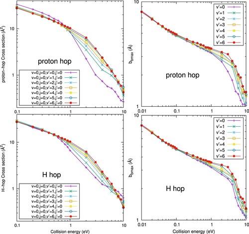
However, above 1 eV the reactive cross sections present important differences among the $v^{\mathrm{\prime }}$ considered, showing that the vibrational excitation has a strong impact on the reactivity. In general, the reactive cross section increases with increasing $v^{\mathrm{\prime }}$, which could be simply understood assuming that ${\mathrm{H}}_2^{+}$ can break more easily. In the left panels of Figure 5 the two main mechanisms to form ${\mathrm{H}}_3^{+}$ are separated as H-hop and proton-hop, corresponding to the fragmentation of ${\mathrm{H}}_2$ or ${\mathrm{H}}_2^{+}$ reactants, respectively. For collision energies below 1 eV, the cross section for the proton-hop mechanism is slightly larger. However, above 3 eV the H-hop cross section is larger for $v^{\mathrm{\prime }}$=0, and the two mechanisms tend to a rather similar value as $v^{\mathrm{\prime }}$ increases. This means that the vibrational excitation of ${\mathrm{H}}_2^{+}$ does not produce significant increase of the proton-hop mechanism. This can be explained looking at the right panels of Figure 5, where the maximum impact parameter, $b_{\max }$, is plotted for each proccess and inital vibrational state. Above 1 eV, $b_{\max }$ increases from $v^{\mathrm{\prime }}$= 0 to $v^{\mathrm{\prime }}$=6, in nearly an identical quantity for the two mechanisms. We conclude that the increase of the cross section when varying $v^{\mathrm{\prime }}$ is due to the growing of the ${\mathrm{H}}_2^{+}$ subunit, whose right turning point increases from 1.25 to 2.12 Å, for $v^{\mathrm{\prime }}$=0 and 6 respectively. Therefore, at energies above 1 eV, when long-range interactions are not able to produce important deviations among the reactants, the size of the two reactants approximately determines the value of the maximum impact parameter. At these higher energies a more complex reaction mechanism occurs, in which ${\mathrm{H}}_2$ may nearly insert in the ${\mathrm{H}}_2^{+}$ bond, specially at high $v^{\mathrm{\prime }}$ excitations.

Figure 5. H-hop and proton-hop cross sections (left panels) and maximum impact parameter, $b_{\max }$, (right panels) for the ${\mathrm{H}}_2$(v=0,j=0) + ${\mathrm{H}}_2^{+}$($v^{\mathrm{\prime }},j^{\mathrm{\prime }}$=0) reaction obtained with QCT calculations for different vibrational states $v^{\mathrm{\prime }}$ of ${\mathrm{H}}_2^{+}$.

3.3. D${}_2$ + D${}_2^{+}$ collisions in PES1

The reactive cross section for the D${}_2$(v, j) + D${}_2^{+}$($v^{\mathrm{\prime }},j^{\mathrm{\prime }}$) collisions is shown in Figure 6 for v = j = 0 and $v^{\mathrm{\prime }}$ = $j^{\mathrm{\prime }}$ = 0. For energies below 1 eV, the results for D${}_2$ + D${}_2^{+}$ closely match those for ${\mathrm{H}}_2$ + ${\mathrm{H}}_2^{+}$. This can be explained in terms of the Langevin model, in which the cross section of Equation (8(8) $\sigma \left(E\right)=\pi (\alpha /E{)}^{1/2}.$(8) ) does not depend on the mass of the reactants. This explains why the reaction cross sections for D${}_4^{+}$ and ${\mathrm{H}}_4^{+}$ are nearly the same.

Figure 6. (a) D${}_2$(v=0,j=0) + D${}_2^{+}$($v^{\mathrm{\prime }}$=0, $j^{\mathrm{\prime }}$=0) reactive cross sections (blue line with open circles) compared with those for ${\mathrm{H}}_2$(v=0,j=0) + ${\mathrm{H}}_2^{+}$($v^{\mathrm{\prime }}$=0,$j^{\mathrm{\prime }}$=0) (red line with open circles) obtained by QCT calculations. The cross section from Janev et. al. [98] for ${\mathrm{H}}_2$ + ${\mathrm{H}}_2^{+}$ reaction is also displayed for comparison (black line with open circles). (b) The difference of each cross section relative to the present ${\mathrm{H}}_2$ + ${\mathrm{H}}_2^{+}$ cross section (open triangles on the coloured line).

However, it should be noted that for reactions involving partially deuterated species, the reaction cross section presents larger differences, as those already reported in the theoretical study of Ref. [60]. The shift of the centre-of-mass with respect to the geometric centre of the two diatomic reagents introduces important differences, specially related to the effect of the rotation. In particular, in the homonuclear neutral ${\mathrm{H}}_2$ or D${}_2$ case for j=0, only the charge-electric dipole term affects the long-range interaction, determining the reactive cross section below 1 eV. In this case, the charge-electric quadrupole term vanishes when integrating over the angular coordinate for the isotropic j=0 case (but not for $j>$ 0).

3.4. Non-adiabatic effects and fit accuracy

The increasing of the ${\mathrm{H}}_2^{+}\left(v^{\mathrm{\prime }}\right)$ vibrational excitation yields to an increase in the reactive cross section. However, this increasing, even for $v^{\mathrm{\prime }}$=6 does not match the new experimental data by Savic et al. [65]. Since the cross section as a function of the $v^{\mathrm{\prime }}$ excitation seems to converge to the value of $v^{\mathrm{\prime }}$=6, here after we shall focus on the two limiting cases, $v^{\mathrm{\prime }}$= 0 and 6.

In order to investigate the role of electronic transitions among the lower electronic states, in this work we use the PESTRIM8×8, comparing it to the results on the PESTRIM1×1 model. The dynamical results obtained for these two potentials are shown in Figure 7, and compared with the data obtained with PES1. All the results present a similar behaviour, with small differences in the logarithmic scale used in the figure. All the results converge to the same value at the lowest collision energy considered here, 1 meV, since all the PESs used in this work have similar long range interactions.

Figure 7. QCT ${\mathrm{H}}_2$(v=0,j=0) + ${\mathrm{H}}_2^{+}$($v^{\mathrm{\prime }}$=6,$j^{\mathrm{\prime }}$=0) $\to$ ${\mathrm{H}}_3^{+}+\mathrm{H}$ reactive cross sections obtained with the PESTRIM8×8 using surface hoping method (blue), the PESTRIM1×1 (red), the PES1 (black) and the new PES-NN (green) potential energy surfaces.

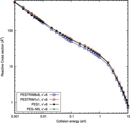
At intermediate energies, between 0.01 and 2 eV, the PESTRIM8×8 and PESTRIM1×1 cross sections are slightly different, showing a small effect of non-adiabatic transitions in the dynamics. Curiously, these non-adiabatic effects seem to produce a decrease on the reactive cross section, in contrast to what is needed to match the values at higher energies of the experimental results of Savic et al. [65].

In Figure 7 we also compare with the cross section obtained with the adiabatic PES1, which nearly matches the results obtained with the adiabatic PESTRIM1×1 up to 3 eV. Above 3 eV, the results obtained with PES1 are higher than those for PESTRIM1×1, showing that the four body term may be important. However, for the new PES-NN, of higher accuracy than PES1, the reaction cross section is nearly identical to that of PESTRIM1×1 for collision energies below 1 eV and very close to those obtained with PESTRIM8×8 for energies above 4 eV. From this comparison we may conclude that the better accuracy of the four body term of the new PES-NN does not improve significantly the differences between the simulated and measured [65] reactive cross-sections.

In order to analyse whether there are other excited states not well described by the TRIM approximation, we have performed ab initio calculations of the four lower electronic states, considering a larger electronic basis set, with extra orbitals added to describe the 2s and 2p electronic states of atomic hydrogen. With this larger basis set, we have found that the energies obtained (extrapolated to the complete basis set) differ only a few tenths of meV with the previous ab initio calculations, and that no higher electronic state appears below 10 eV.

3.5. Double fragmentation and reaction mechanism

For ${\mathrm{H}}_2^{+}(v^{\mathrm{\prime }}=6)$ the double fragmentation (DF) channel opens at ≈ 2 eV, as it is shown in the left panel of Figure 8. The opening of this channel occurs approximately for values where the extra energy of $v^{\mathrm{\prime }}$=6, 1.67 eV, is added to the D${}_0$ of ${\mathrm{H}}_2^{+}$, 2.65 eV

Figure 8. QCT ${\mathrm{H}}_2($v$=0,$j$=0)$ + ${\mathrm{H}}_2^{+}($v'$=6,$j'$=0)$ $\to$ ${\mathrm{H}}_2$ + ${\mathrm{H}}^{+}+\mathrm{H}$ (DF channel) reactive cross sections (left panel) and total cross section (formation of ${\mathrm{H}}_3^{+}$ and DF channel, in right panel) obtained with the PESTRIM8×8 using surface hoping method (blue), the PESTRIM1×1 (red) and the new PES-NN ( green) potential energy surfaces. The experimental results are those of Refs. [54], [62] and [65] and.

If we add the DF channel contribution to the production of ${\mathrm{H}}_3^{+}$, as shown in the right panel of Figure 8 the cross section increases considerably, reaching a very good agreement with the new experimental data of Savic et al. [65] above 3 eV.

The main mechanism giving rise to the DF channel consists of three steps, as it is shown in the left panels of Figure 9. First, a highly vibrationally excited ${\mathrm{H}}_4^{+}$ intermediate is formed by insertion of ${\mathrm{H}}_2$ in the elongated ${\mathrm{H}}_2^{+}$, which lives short time. Second, a first H atom is ejected (in the Figure is atom 2 with charge 0), forming a very excited (${\mathrm{H}}_3^{+}$)${}^{\ast }$, which lives from 80 to 160 fs, approximately. In the third step, one of the atoms of ${\mathrm{H}}_3^{+}$ (atom 4 in the Figure) dissociates, carrying the positive charge, thus leading to neutral ${\mathrm{H}}_2$. Since this third step occurs much later, it could explain that experimentally the metastable (${\mathrm{H}}_3^{+}$)${}^{\ast }$ would be detected together with more stable ${\mathrm{H}}_3^{+}$ products. It is also important to notice that the energy transfer among particles of identical mass is possibly overestimated in a classical treatment, as the one used in this work. If this is the case, it would support the inclussion of the DF cross section as a part of the total reaction cross section. Quantum calculations are needed to solve this problem, but they are rather challengig at the high energy considered.

Figure 9. Two typical trajectories leading to double fragmentation (DF), as a function of the collision time in fs. Lower panels show the charge on each atom (Mulliken population) for the ground electronic state. Middle panels shows the energies of the four lower electronic states. Upper panels show some characteristic internuclear distances needed to characterise the trajectory. $R_{\mathrm{ij}}$ refers to the distance between atom ${\mathrm{H}}_i$ and ${\mathrm{H}}_j$.

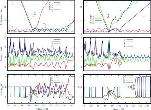
The right panels of Figure 9 show another DF mechanism: in this case ${\mathrm{H}}_2$ and ${\mathrm{H}}_2^{+}$ are produced at 70-80 fs. ${\mathrm{H}}_2^{+}$ is vibrationally very excited and dissociates later, at ≈100–110 fs. In this case, there are two degenerate electronic states, each one corresponding to the charge in one of the ejected atoms, at long distances from the ${\mathrm{H}}_2$ fragment. In the ground electronic state, shown in the lower panels, the charge is exchanged between the two identical atoms, because of this degeneracy, and shows the nature of the surface hopping occurring in the products channel when including several electronic states (PESTRIM8×8). The electronic transition occurs among degenerate electronic states describing ${\mathrm{H}}_2$ + $\mathrm{H}{\mathrm{H}}^{+}$ and ${\mathrm{H}}_2$ + ${\mathrm{H}}^{+}+\mathrm{H}$ products, what explains the small effect of including electronic transitions in the reaction dynamics.

In addition, the charge transfer in the entrance channel occurs between ${\mathrm{H}}_2$ and ${\mathrm{H}}_2^{+}$, when the two reactants have the same internuclear distance (see bottom panels of Figure 9). In this situation there is a degeneracy between the two lower adiabatic states, as discussed in detail in Ref. [60].

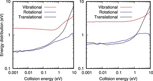
The energy distributions of the ${\mathrm{H}}_3^{+}+\mathrm{H}$ products are shown in Figure 10, and it is nearly quantitatively the same for all the PESs. The energy difference between the two vibrational states of ${\mathrm{H}}_2^{+}$($v^{\mathrm{\prime }}$= 0 and 6) is approximately 1.4 eV, close to the exoergicity. For low collision energies, 0.1-1 meV, the initial vibrational energy of ${\mathrm{H}}_2^{+}$( $v^{\mathrm{\prime }}$= 6) is 1.40 eV higher than that of ${\mathrm{H}}_2^{+}$ ($v^{\mathrm{\prime }}$= 0), and the vibrational energy of the corresponding ${\mathrm{H}}_3^{+}$ products is also higher, but only by ≈ 0.9 eV. Therefore the remaining 0.4 eV are nearly equally distributed between the rotational and translational energies of the products. Rotational energy increases with collision energy, except for the $v^{\mathrm{\prime }}$= 6 above 1 eV, where rotational excitation reaches a plateau and seems to start decreasing. The translational energy always increases for $v^{\mathrm{\prime }}$= 0, while for $v^{\mathrm{\prime }}$= 6 it slightly decreases below 0.1 eV, and then increases again. The vibrational energy of products shows two different behaviours: below ≈ 0.7 eV, the vibrational energy slightly decreases ($v^{\mathrm{\prime }}$=0) or remains constant ($v^{\mathrm{\prime }}$=6); above this energy the vibrational energy increases sharply.

Figure 10. Vibrational, rotational and translational energy distributions of the ${\mathrm{H}}_3^{+}+\mathrm{H}$ products, as a function of the collision energy for the ${\mathrm{H}}_2(v=0)$ + ${\mathrm{H}}_2^{+}\left(v^{\mathrm{\prime }}\right)$ collisions, for $v^{\mathrm{\prime }}$=0 (left panel) and $v^{\mathrm{\prime }}$=6 (right panel). The origin of energy is in the bottom of the well of the ${\mathrm{H}}_3^{+}$ products. The initial vibrational energies of the reactants is 0.413 and 1.673 eV for the $v^{\mathrm{\prime }}$= 0 and 6, respectively, with respect to the minimum of each fragment. The potential energy difference between reactants and products is 1.816 eV, and when ZPE are accounted for, the exoergicity of the present PES becomes 1.688 eV.

Such behaviour allows to assign two different reaction mechanisms. Below ≈ 0.7 eV, the impact parameter (in Figure 5) is large, supporting a stripping mechanism, in which the long range interactions attract the reactants to each other, originating orbits enhancing the relative angular momentum between the two reactants. Above ≈ 0.7 eV, however, the impact parameter is rather small, and the reaction occurs by an insertion mechanism, in which the ${\mathrm{H}}_3^{+}$ is greatly excited vibrationaly, specially as initial vibrational and translational energy of the reactants increases.

The dissociation energy of ${\mathrm{H}}_3^{+}$ is 4.34 eV, very close to the value reported by [99] of 4.35 eV, and the average vibrational energy distribution of ${\mathrm{H}}_3^{+}$ reaches values in the 4-5 eV interval, $i.e.$ values above the dissociation energy explaining why ${\mathrm{H}}_3^{+}$ dissociates, leading to the DF channel.

4. Plasma modelling

To model the hydrogen plasma, we shall consider a gas-discharge vessel of cylindrical symmetry, so that only z, parallel to the central axis, and R, the distance from the centre to the walls, will be considered, with the cylinder of infinite length in this case. The gas is initially in the form of neutral ${\mathrm{H}}_2$, and after the discharge ignition new species are formed, H, ${\mathrm{H}}^{+}$, ${\mathrm{H}}_2^{+}$, ${\mathrm{H}}_3^{+}$ and electrons. ${\mathrm{H}}^{-}$ is neglected under the conditions considered here. To model the abundance of these species in the stationary condition we use a model similar to those already described previously [41, 100], which is outlined in the Appendix B, including all the processes listed in Table A1, in which the vibrations of molecular species, ${\mathrm{H}}_2$, ${\mathrm{H}}_2^{+}$ and ${\mathrm{H}}_3^{+}$ are not considered.

The plasma model is done for pure hydrogen and pure deuterium gases. For modelling deuterium plasma, the cross sections for electron collisions and radiative transitions of D species are used by those of H species.

The cross section for ${\mathrm{H}}_2$ + ${\mathrm{H}}_2^{+}$ and D${}_2$ + D${}_2^{+}$ reactive collisions calculated in this work are included in the models presented below. The plasma modellings are also done using the cross section by Janev et al. (2003) [98], which are compared with the present calculations in Figure 6.

Here, the electron temperature $T_e=5.55$ eV and electron density $n_e=2.07\times {10}^{12}$ cm${}^{-3}$ are used, which were measured by a Langmuir probe for D plasma in a long cylindrical vessel [39]. The molecular temperature is set to $T_m$= 0.026 eV (300 K) and the atomic temperature is $T_a$ = 0.052 eV (600 K). At these realistic temperatures, the relevant energies are below $E_{\mathrm{col}}$= 1 eV, so that the ${\mathrm{H}}_2^{+}$ vibrational excitation has no significant effect.

Figure 11 shows the resulting population densities of D and H species depending on the cross section used. We can note, the ${\mathrm{D}}_3^{+}$ and ${\mathrm{H}}_3^{+}$ population densities vary significantly with the cross section used, while other species are nearly unchanged, as shown in Figure 11. The D${}_3^{+}$ and ${\mathrm{H}}_3^{+}$ population density changes are also summarised in Table 3. It is worth noting that the main depopulating mechanism for ${\mathrm{H}}_3^{+}$ density is the diffusion process (given in the last term of Equation A7(A7) $\begin{array}{rl}\frac{\mathrm{d}{n}_i}{\mathrm{d}t}& ={\delta }_{i41}(n_e{\alpha }_{14}{n}_{43}+\frac{Q_{\mathrm{in}}}{V}\times 4.48\times {10}^{17}+\frac{{\gamma }^{\mathrm{\prime }}}{\tau }{n}_1\\ & +\sum _{j=42}^{43}{\zeta }_{\mathrm{mj}}{\left(\frac{\mu }{R}\right)}^2{D}_{\mathrm{Aj}}{n}_j+{\zeta }_{m{H}^{+}}{\left(\frac{\mu }{R}\right)}^2{D}_{A{H}^{+}}{n}_{H^{+}})\\ & -n_e(\sum _{k=5}^8{\alpha }_k{\delta }_{i41}{n}_i+\sum _{k=9}^{12}{\alpha }_k{\delta }_{i42}{n}_i+\sum _{k=13}^{15}{\alpha }_k{\delta }_{i43}{n}_i)\\ & +{\delta }_{i42}(n_e{\alpha }_8-n_{41}{\alpha }_{16})n_i\\ & +{\delta }_{i43}{n}_{41}{\alpha }_{16}{n}_{42}-{\delta }_{i41}{\alpha }_{16}{n}_{42}{n}_i\\ & -\frac{Q}{V}{n}_i-(1-{\delta }_{i41}){\left(\frac{\mu }{R}\right)}^2{D}_{\mathrm{Ai}}{n}_i.\end{array}$(A7) ), while the electron impact processes (${\mathrm{H}}_3^{+}+e$ in Table A1) only contribute to the depopulation in a small fraction.

Figure 11. The population densities of D and H species by modelling using the different cross sections shown in Figure 6. In the inset, the labels of x-axis correspond to the cross sections used given by the upper number in the legends of the main graph.

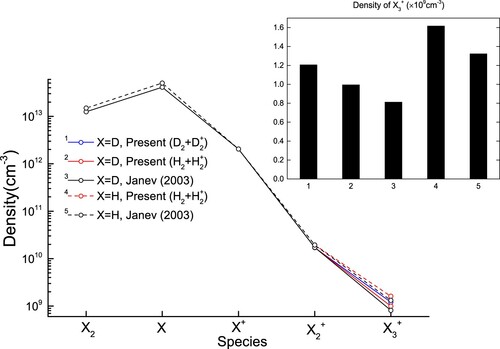
Table 3. Rate coefficients for D${}_2$(v=0,j=0) + D${}_2^{+}$($v^{\mathrm{\prime }}$=0,$j^{\mathrm{\prime }}$=0) reaction and the modelled density of D${}_3^{+}$ depending on the cross sections shown in Figure 6(a).

	Present D${}_3^{+}$	Present ${\mathrm{H}}_3^{+}$	${\mathrm{H}}_3^{+}$ by Janev et al. [98]
${\alpha }_{16}$ (cm${}^3$/s)	$2.38\times {10}^{-9}$	$1.96\times {10}^{-9}[2.76\times {10}^{-9}]$	$1.59\times {10}^{-9}[2.25\times {10}^{-9}]$
n${}_{D_3^{+}}$ (cm${}^{-3}$)	$1.21\times {10}^9$	$9.95\times {10}^8[1.62\times {10}^9]$	$8.12\times {10}^8[1.32\times {10}^9]$

Note: The values in the $\left[\right]$ represent for the densities of ${\mathrm{H}}_3^{+}$ and the rate coefficient for ${\mathrm{H}}_2$(v=0,j=0) + ${\mathrm{H}}_2^{+}$($v^{\mathrm{\prime }}$=0,$j^{\mathrm{\prime }}$=0) reaction.

The present cross section for D${}_2$ + D${}_2^{+}$ is larger than that for ${\mathrm{H}}_2$ + ${\mathrm{H}}_2^{+}$ by $\sim 2$% at low collision energy, below $\sim 0.026$ eV. On the contrary for collision energies above 1 eV, the cross section for deuterium is ≈ 20$\mathrm{\%}$ lower than that of pure hydrogen reaction, as shown in Figure 6.b. For ${\mathrm{H}}_2$ + ${\mathrm{H}}_2^{+}$, the cross section by Janev et. al [98] is smaller than the present ones by $20\sim 30$ % below 1 eV, but the difference is enlarged up to 100 % (black triangle) at the collision energy over $\sim 1.0$ eV as shown in Figure 6(b).

The reaction rate coefficient calculated at the molecular temperature, $T_m=0.026$ eV, for pure deuterium is ≈ 20$\mathrm{\%}$ larger than for pure hydrogen, and is also larger than those obtained from Janev et al. [98] by $\sim 40$ %, as listed in Table 3. These differences have a rather linear impact on the resulting D${}_3^{+}$ and ${\mathrm{H}}_3^{+}$ population densities, whose difference varies proportionally to the difference between the rate coefficients listed in Table 3.

As a result, the use of the present results for D${}_2$ + D${}_2^{+}$ and ${\mathrm{H}}_2$ + ${\mathrm{H}}_2^{+}$ leads to significantly different D${}_3^{+}$ and ${\mathrm{H}}_3^{+}$ population densities compared with the widely used cross section for ${\mathrm{H}}_2$ + ${\mathrm{H}}_2^{+}$ [98] in this plasma modelling. It should also be noted that the use of the cross section for ${\mathrm{H}}_2$ + ${\mathrm{H}}_2^{+}$ instead of that for D${}_2$ + D${}_2^{+}$ in the modelling of D plasma can give rise to unreliable population density of D${}_3^{+}$, even though the difference between the two cross sections is small, due to the rate coefficient sensitivity to the cross section at the low collision energy.

When T${}_e$ and n${}_e$ are reduced to 3 eV and 1.5 × 10${}^{10}$ (cm${}^{-3}$), respectively, and the molecular pressure is increased by about 10 times, the amount of X${}_3^{+}$ (X=D, H) becomes dominant over those of X${}_{1,2}^{+}$ ions. These conditions are similar to those reported by Tanarro and Herrero [32], who also find a significant increase of the ${\mathrm{H}}_3^{+}$ population. This relative increase of the X${}_3^{+}$ density is mostly attributed to that the rate coefficient of X${}_2$ + e collision populating X${}_2^{+}$ becomes smaller than the rate coefficient of X${}_2$ + X${}_2^{+}$ collision depopulating X${}_2^{+}$.

However, the density of X${}_3^{+}$ in this high pressure is less sensitive to the change of the cross section for X${}_2$ + X${}_2^{+}$ collision than in the low pressure. This is due to the fact that the increased X${}_2$ + X${}_2^{+}$ rate coefficient is accompanied by the decreased X${}_2^{+}$ quantity since X${}_2$ + X${}_2^{+}$ collision is the main depopulation process for X${}_2^{+}$, which leads to the little change of the X${}_3^{+}$ formation. While in the previous case of low pressure, the main depopulating of X${}_2^{+}$ does not come from the X${}_2$ + X${}_2^{+}$ collision but from X${}_2^{+}$ + e collision and the density of X${}_2^{+}$ is not affected by the X${}_2$ + X${}_2^{+}$ rate coefficient. Thus the density of X${}_3^{+}$ in the low pressure case is more sensitive to the change of the cross section for X${}_2$ + X${}_2^{+}$ collision than in the high pressure limit having its linear dependency on the rate coefficient mentioned above.

On the other hand, when the molecular temperature is increased from $T_m$ = 0.026 eV (300 K) to $T_m$= 4.2 eV (50,000 K), the rate coefficient for the present cross section of ${\mathrm{H}}_2$(v=0,j=0) + ${\mathrm{H}}_2^2$($v^{\mathrm{\prime }}$= 0,$j^{\mathrm{\prime }}$= 0) differs from that for the cross section by Janev et al. [98] only by about 20 %. However, the cross section of ${\mathrm{H}}_2$(v=0,j=0) + ${\mathrm{H}}_2^{+}$($v^{\mathrm{\prime }}$=6,$j^{\mathrm{\prime }}$=0), shown in Figure 8, is much larger than that of ${\mathrm{H}}_2$(v=0,j=0) + ${\mathrm{H}}_2^{+}$($v^{\mathrm{\prime }}$=0,$j^{\mathrm{\prime }}$=0) by Janev et al. [98] at collision energies higher than 1 eV. The difference between the rate coefficients using these two cross sections is as much as 10-170 % at the temperature range $T_m$ = 0.026-4.0 eV. The larger differences are found at higher $T_m$, becoming over  40 % above 1 eV. Hence the high $v^{\mathrm{\prime }}$ state of ${\mathrm{H}}_2^{+}$ can contribute to the population of ${\mathrm{H}}_3^{+}$ much more than the $v^{\mathrm{\prime }}$=0 state. This was analysed by replacing the ${\mathrm{H}}_2$(v=0,j=0) + ${\mathrm{H}}_2^{+}$($v^{\mathrm{\prime }}$=0,$j^{\mathrm{\prime }}$=0) reactive rate coefficient by that obtained for ${\mathrm{H}}_2$(v=0,j=0) + ${\mathrm{H}}_2^{+}$($v^{\mathrm{\prime }}$=6,$j^{\mathrm{\prime }}$=0) collision. To further analyse the effect of ${\mathrm{H}}_2^{+}$ vibrational state, new plasma models need to be developed, increasing considerably in complexity for the quantity of processes included.

5. Conclusion

In this work a detailed study on the ${\mathrm{H}}_2$ + ${\mathrm{H}}_2^{+}$($v^{\mathrm{\prime }}$) $\to$ ${\mathrm{H}}_3^{+}+\mathrm{H}$ reactive cross section has been done using a quasi-classical treatment, for collision energies from 1 meV up to 10 eV and for several vibrational states of the ${\mathrm{H}}_2^{+}$ reactants and several isotopic variations. To this aim, new potential energy surfaces have been developed, one to include non-adiabatic transitions (PESTRIM8×8) and another to increase the accuracy in the whole energy range up to 17 eV (PES-NN). In all cases, it is found that from 1 meV to ≈ 0.5-1 eV the cross section behaves according to a Langevin law for charge induced-dipole long range interactions. For energies above 1 eV, the simulated cross section decreases fast, below the Langevin limit, for all initial vibrational states of ${\mathrm{H}}_2^{+}$($v^{\mathrm{\prime }}$). However, for E > 1 eV, the reactive cross section exhibits a considerable increase with increasing $v^{\mathrm{\prime }}$, and the results seems to converge at $v^{\mathrm{\prime }}$=6.

It is found that the reactive cross section for $v^{\mathrm{\prime }}$=6, summing the ${\mathrm{H}}_3^{+}+\mathrm{H}$ and ${\mathrm{H}}_2+\mathrm{H}{\mathrm{H}}^{+}$ channels, match very well the recent experimental measurements by Savic et al. [65], and also previous measurements [54, 62], describing a broad energy interval from 0.5 meV to 10 eV. Moreover, the fact that for collision energies above 1 eV the measured reactive cross section show different values in different experiments, can be explained by a different vibrational excitation of ${\mathrm{H}}_2^{+}$ achieved in each experimental setup.

Experimentally, the ${\mathrm{H}}_3^{+}$ products are measured [65]. The fact that in the QCT simulations, the cross section for the double fragmentation channel, ${\mathrm{H}}_2+\mathrm{H}{\mathrm{H}}^{+}$, needs to be considered to get an agreement with the new experimental results can be explained by a classical artifact, since QCT method usually overstimate the energy transfer, specially dealing with systems with equal masses.

The new reactive cross sections obtained for ${\mathrm{H}}_2$ + ${\mathrm{H}}_2^{+}$($v^{\mathrm{\prime }}$) and D${}_2$ + D${}_2^{+}$ have been included in a plasma model together with the widely used cross section [98]. The resulting population densities of ${\mathrm{H}}_3^{+}$ and D${}_3^{+}$ are proportional to the rate coefficient, which in turn indicates the sensitivity of the population density to the adopted cross section. The new cross sections for vibrational sates ($v^{\mathrm{\prime }}$) of ${\mathrm{H}}_2^{+}$ will be useful for the state-resolved CR modelling in plasma with higher molecular temperature, where higher collision energies (above 0.7 eV) become significant and the differences in the reactivity of the vibrationally excited ${\mathrm{H}}_2^{+}$ will become important.

Acknowledgements

We thank Profs. S. Schlemmer and I. Savić for providing us the experimental measurement data and for very fruitfull discussions. Also, we acknowledge Prof. I. Tanarro for a carefull reading of the manuscript and very valuable comments and discussions, and Prof. F. Merkt for providing their experimental data. We acknowledge computing time at Cibeles (CCC-UAM) and Trueno (CSIC).

Disclosure statement

No potential conflict of interest was reported by the author(s).

Additional information

Funding

The research leading to these results has received fundings from MICINN (Spain) [grant number PID2021-122549NB-C2], and from KAERI Institutional Program (Korea) [grant number 524410-22]. Pablo del Mazo-Sevillano acknowledge the finantial support from Ministerio de Universidades and Universidad Autónoma de Madrid, Plan de Recuperación, Transformación y Resiliencia [Margarita Salas fellowship, Ref. CA4/RSUE/2022-00287].

Appendix A.

N-body permutational invariant polynomials

In this section we provide a definition of a permutational invariant polynomial in terms of graph theory, which we latter use as a way of filtering the N-body polynomials from a general set of PIP.

A graph is a collection of vertices and edges ($\mathcal{G}=(V,E)$) [101]. In an undirected graph the edges are non-ordered pairs of vertices. An undirected graph is said to be connected if every pair of vertices are joined by a path.

A relation can be established between the polynomials $P_n$ in Equation (5(5) $P_n=\hat{S}\prod _{i=1}^{N_d}{p}_i^{l_i^n}\left(r_i\right)$(5) ) and an undirected graph, where the vertices represent the particles and the edges the monomials between them.

For instance, the following polynomial (A1) $P=p_{12}{p}_{34}$(A1) can be expressed as the following graph:

This corresponds to a disconnected graph since there are various pairs of vertices which are not reachable, for instance from vertex 2–3. An example of a polynomial whose graph is connected is: (A2) $P=p_{12}{p}_{13}{p}_{34}$(A2)

A polynomial P is said to be a N-body polynomial if its corresponding undirected graph is connected. Any other polynomial that arises as $\hat{S}P$ with $\hat{S}$ being any operation of a permutation group will be a N-body polynomial if P is. Note that the effect of a permutation operation in the graph only affects the order of the vertices and relabel of the edges: (A3) $P^{\mathrm{\prime }}={\hat{S}}_{14}P=p_{42}{p}_{34}{p}_{31}$(A3)

Given a graph, there are simple algorithms as Depth-First Search (DFS) [102] to compute whether it is a connected graph or not, which recursively traverses the graph marking each visited vertice. If at the end of the execution all nodes were visited, the graph is connected. There exist a finite number of connected N-vertices undirected graphs which can be evaluated using the recursive formula [103]: (A4) $C_n=2^{(\genfrac{}{}{0ex}{}{n}{2})}-\frac{1}{n}\sum _{k=1}^{n-1}k(\genfrac{}{}{0ex}{}{n}{k})2^{(\genfrac{}{}{0ex}{}{n-k}{2})}{C}_k$(A4) These numbers are tabulated for N up to 16 in [104]. One should note that the number of connected undirected graphs increases fast, for instance for a set of six vertices there exist 26704 of those, so in practice an upper limit on the number of edges has to be set.

At this point we have the tools to determine the number of N-body polynomials, as well as, given a polynomial, to determine if it is N-body. If the system presents some kind of permutational symmetry, a minimal set of N-body PIP will be generated by projecting the above polynomials onto the totally symmetric irreducible representation of the permutation group. The dimension of the minimal PIP set is necessarily lower or equal to the minimal one of polynomials, as many of them are related by permutation operations. Note that we never mentioned the exponents l of the monomials, since they play no role in the graph construction. Hence, what we have defined up to here is a generator of N-body polynomials or PIPs. Following the general procedure, we are now free to set the desired maximum polynomial degree and produce the combinations of monomial exponents l to generate a finite set of functions.

Appendix B.

Method for the plasma model

The method used to model the plasma is similar to that previously described [41, 100], in which each particle's level i density $n_i$ can be solved from a continuity equation (A5) $\frac{\mathrm{d}{n}_i}{\mathrm{d}t}=\frac{\mathrm{\partial }{n}_i}{\mathrm{\partial }t}+▽\cdot \left(\mathrm{D▽}{n}_i\right)=\frac{\delta n_i}{\mathrm{\delta t}},$(A5) where D denotes diffusion coefficient and the right hand side is the net particle source and sink term by collisional-radiative (CR) process and particle flux into and out a volume. In steady state of $\mathrm{\partial }{n}_i/\mathrm{\partial t}=0$, the density balance equations for a long cylindrical vessel plasma can be expressed as follows. For atomic levels of $\mathrm{H}(n_i,i=1-40)$ (A6) $\begin{array}{rl}\frac{\mathrm{d}{n}_i}{\mathrm{d}t}& =\sum _{j>i}^{40}{\eta }_{\mathrm{ji}}{A}_{\mathrm{ji}}{n}_j-(\sum _{j<i}{\eta }_{\mathrm{ij}}{A}_{\mathrm{ij}}+\frac{Q}{V}+\frac{\gamma }{\tau }{\delta }_{i1})n_i\\ & +n_e(\sum _{j\ne i}{\alpha }_{1,\mathrm{ji}}{n}_j-\sum _{j\ne i}{\alpha }_{1,\mathrm{ij}}{n}_i-{\alpha }_{2i}{n}_i+{\alpha }_{41}{n}_{H^{+}})\\ & +n_e({\alpha }_{5i}+{\alpha }_6{\delta }_{i2}+{\alpha }_7{\delta }_{i1})n_{41}\\ & +n_e({\alpha }_{9i}+{\alpha }_{10i}+{\alpha }_{12i})n_{42}\\ & +n_e({\alpha }_{13}{\delta }_{i1}+{\alpha }_{14}{\delta }_{i2}+{\alpha }_{15}{\delta }_{i1})n_{43}+n_{41}{\alpha }_{16}{\delta }_{i1}{n}_{42}\\ & +(\sum _{j=42}^{43}{\zeta }_{\mathrm{aj}}{\left(\frac{\mu }{R}\right)}^2{D}_{\mathrm{Aj}}{n}_j+{\zeta }_{a{H}^{+}}{\left(\frac{\mu }{R}\right)}^2{D}_{A{H}^{+}}{n}_{H^{+}}){\delta }_{i1},\end{array}$(A6) and for species ${\mathrm{H}}_2(n_i,i=41)$, ${\mathrm{H}}_2^{+}(n_i,i=42)$, and ${\mathrm{H}}_3^{+}(n_i,i=43)$ (A7) $\begin{array}{rl}\frac{\mathrm{d}{n}_i}{\mathrm{d}t}& ={\delta }_{i41}(n_e{\alpha }_{14}{n}_{43}+\frac{Q_{\mathrm{in}}}{V}\times 4.48\times {10}^{17}+\frac{{\gamma }^{\mathrm{\prime }}}{\tau }{n}_1\\ & +\sum _{j=42}^{43}{\zeta }_{\mathrm{mj}}{\left(\frac{\mu }{R}\right)}^2{D}_{\mathrm{Aj}}{n}_j+{\zeta }_{m{H}^{+}}{\left(\frac{\mu }{R}\right)}^2{D}_{A{H}^{+}}{n}_{H^{+}})\\ & -n_e(\sum _{k=5}^8{\alpha }_k{\delta }_{i41}{n}_i+\sum _{k=9}^{12}{\alpha }_k{\delta }_{i42}{n}_i+\sum _{k=13}^{15}{\alpha }_k{\delta }_{i43}{n}_i)\\ & +{\delta }_{i42}(n_e{\alpha }_8-n_{41}{\alpha }_{16})n_i\\ & +{\delta }_{i43}{n}_{41}{\alpha }_{16}{n}_{42}-{\delta }_{i41}{\alpha }_{16}{n}_{42}{n}_i\\ & -\frac{Q}{V}{n}_i-(1-{\delta }_{i41}){\left(\frac{\mu }{R}\right)}^2{D}_{\mathrm{Ai}}{n}_i.\end{array}$(A7) The density of ${\mathrm{H}}^{+}$, $n_{H^{+}}$ is deduced from the quasi neutrality condition (A8) $n_e=n_{H^{+}}+n_{42}+n_{43}.$(A8) The electron density, $n_e$, is assumed to have a radial distribution close to a Bessel-type profile for the ambipolar-diffusion regime considered here and applying the Bohm criterion as boundary conditions between the plasma and the vessel walls with μ = 2.405 for an infinite cylinder of the effective radius of R [34, 100]. The effective R is set as 40 cm for our plasma device.

Diffusion time τ for H atom in the device of radius $R_d$ is given by $\tau =2R_d/v_{\mathrm{th}}$ with the thermal velocity $v_{\mathrm{th}}=2\sqrt{2T_a/\pi M_H}$ for atomic temperature $T_a$ and the hydrogen mass $M_{\mathrm{H}}$. The wall recombination coefficient γ is given as the empirical expression $\gamma =0.151\exp (-1.09\times {10}^3/T_m)$ [105], with $T_m$ being the temperature of ${\mathrm{H}}_2$ molecule.

Under the ambipolar diffusion assumption [106] the diffusion coefficient $D_{A{H}^{+}}$ for ${\mathrm{H}}^{+}$ is given by (A9) $D_{A{H}^{+}}=T_e{K}_1^0\left(\frac{760}{p}\frac{T_m}{273}\right),$(A9) where $p=n_{H_2}{T}_m$ is in Torr and the electronic temperature $T_e$ is in eV. The reduced mobility $K_1^0\left({\mathrm{cm}}^2{\mathrm{V}}^{-1}{\mathrm{s}}^{-1}\right)$ for ${\mathrm{H}}^{+}$ and D${}^{+}$ are 15.9 and 11.2, respectively [107]. The diffusion coefficients for ${\mathrm{H}}_2^{+}$ and ${\mathrm{H}}_3^{+}$ are given with the relation $D_{A{H}^{+}}:D_{A{H}_2^{+}}:D_{A{H}_2^{+}}=1:\sqrt{2}/\sqrt{3}:\sqrt{5}/3$ [105].

The conversion coefficients from H ions into H atom (${\zeta }_a$) and ${\mathrm{H}}_2$ molecule (${\zeta }_m$) on the wall are taken from [108]. The conversion coefficient ${\gamma }^{\mathrm{\prime }}$ from H atom to ${\mathrm{H}}_2$ molecule on the wall is also taken from [108]. $Q_{\mathrm{in}}$, Q and V denote the gas flow rate of ${\mathrm{H}}_2$ in the inlet, the pumping rate in the outlet and the volume of the plasma device, respectively. $Q_{\mathrm{in}}$, Q and V are given by 600 sccm (standard cubic centimeters per minute), 4800 lps (liter per second) and 2.64×10${}^6$ cm${}^3$, respectively.

The CR processes and the rate coefficient α notations are listed in Table A1 with the references of the collision cross section and the radiative transition rate. The escaping factor η for radiation trapping in optically thick plasma is given as that for the infinite long cylinder [109].

Table B1. Collisional-radiative reactions and the rate coefficients considered in our plasma CRM.

Reaction	Rate coefficient
$H(n\ge 1)+e\leftrightarrow H(n^{\mathrm{\prime }}>n)+e$	${\alpha }_1$ [98]
$H(n\ge 1)+e\leftrightarrow H^{+}+2e$	${\alpha }_2$ [98]
$H(n\le 40)\to H(n^{\mathrm{\prime }}<n)+\mathrm{h\nu }$	$A_{\mathrm{ij}}$ [110]
$H^{+}+e\to H(n\le 40)+\mathrm{h\nu }$	${\alpha }_4$ [98]
$H_2+e\to H(n=1)+H(n^{\mathrm{\prime }}\le 3)+e$	${\alpha }_5$ [111]
$H_2+e\to 2H(n=2)+e$	${\alpha }_6$ [111]
$H_2+e\to H^{+}+H(n=1)+2e$	${\alpha }_7$ [98]
$H_2+e\to H_2^{+}+2e$	${\alpha }_8$ [98]
$H_2^{+}+e\to H(n=1)+H(n^{\mathrm{\prime }}\ge 2)$	${\alpha }_9$ [111]
$H_2^{+}+e\to H^{+}+H(n\le 2)+e$	${\alpha }_{10}$ [111]
$H_2^{+}+e\to 2H^{+}+2e$	${\alpha }_{11}$ [111]
$H_2^{+}+e\to H_2^{\ast }\to H(n=1)+H(n^{\mathrm{\prime }}\ge 2)$	${\alpha }_{12}$ [98]
$H_3^{+}+e\to 3H(n=1)$	${\alpha }_{13}$ [111]
$H_3^{+}+e\to H_2+H(n=2)$	${\alpha }_{14}$ [111]
$H_3^{+}+e\to H^{+}+2H(n=1)+e$	${\alpha }_{15}$ [111]
$H_2+H_2^{+}\to H_3^{+}+H(n=1)$	${\alpha }_{16}$ [98]

From the cross section the rate coefficient is obtained as (A10) $\alpha =〈\sigma \left(v_{12}\right)v_{12}〉$(A10) as the averaging over the relative velocity $v_{12}$ distribution. When the colliding particles of the masses $m_1$ and $m_2$ have the Maxwellian energy distribution with temperatures $T_1$ and $T_2$ the rate coefficient α can be expressed as [112] (A11) $\alpha \left(T_{12}\right)=\frac{4}{\sqrt{\pi }{v}_{T_{12}}^3}{\int }_0^{\mathrm{\infty }}\sigma \left(v_{12}\right)\exp (-(v_{12}/v_{T_{12}}{)}^2)v_{12}^3\mathrm{d}{v}_{12},$(A11) where $\begin{array}{rl}{T}_{12}& =(m_2{T}_1+m_1{T}_2)/(m_1+m_2)\text{ and }\\ v_{T_{12}}& =\sqrt{2(m_1+m_2)T_{12}/m_1{m}_2}\end{array}$for temperatures in eV. For electron collisions $T_{12}=T_e$ and $v_{T_{12}}=\sqrt{2T_e/m_e}$, with $M_e$ being the electron mass. The Maxwellian rate coefficient ${\alpha }_{16}$ for the heavy particle collision ${\mathrm{H}}_2$ + ${\mathrm{H}}_2^{+}\to$ ${\mathrm{H}}_3^{+}+\mathrm{H}$(n = 1) is obtained with $T_1=T_2=T_m$ and $m_1=m_2=2M_{\mathrm{H}}$.

The balance equations of $\mathrm{d}{n}_i/\mathrm{d}t=0$ including the nonlinear terms of ${\eta }_{\mathrm{ij}}\left(n_i\right)$, ${\alpha }_{16}{n}_{41}{n}_{42}$ and $D_A\left(n_{41}\right)$ are solved by the multidimensional secant Broyden's method [113] setting the initial $n_i$ as the solution of the linear part of Equations (A6(A6) $\begin{array}{rl}\frac{\mathrm{d}{n}_i}{\mathrm{d}t}& =\sum _{j>i}^{40}{\eta }_{\mathrm{ji}}{A}_{\mathrm{ji}}{n}_j-(\sum _{j<i}{\eta }_{\mathrm{ij}}{A}_{\mathrm{ij}}+\frac{Q}{V}+\frac{\gamma }{\tau }{\delta }_{i1})n_i\\ & +n_e(\sum _{j\ne i}{\alpha }_{1,\mathrm{ji}}{n}_j-\sum _{j\ne i}{\alpha }_{1,\mathrm{ij}}{n}_i-{\alpha }_{2i}{n}_i+{\alpha }_{41}{n}_{H^{+}})\\ & +n_e({\alpha }_{5i}+{\alpha }_6{\delta }_{i2}+{\alpha }_7{\delta }_{i1})n_{41}\\ & +n_e({\alpha }_{9i}+{\alpha }_{10i}+{\alpha }_{12i})n_{42}\\ & +n_e({\alpha }_{13}{\delta }_{i1}+{\alpha }_{14}{\delta }_{i2}+{\alpha }_{15}{\delta }_{i1})n_{43}+n_{41}{\alpha }_{16}{\delta }_{i1}{n}_{42}\\ & +(\sum _{j=42}^{43}{\zeta }_{\mathrm{aj}}{\left(\frac{\mu }{R}\right)}^2{D}_{\mathrm{Aj}}{n}_j+{\zeta }_{a{H}^{+}}{\left(\frac{\mu }{R}\right)}^2{D}_{A{H}^{+}}{n}_{H^{+}}){\delta }_{i1},\end{array}$(A6) ) and (A7(A7) $\begin{array}{rl}\frac{\mathrm{d}{n}_i}{\mathrm{d}t}& ={\delta }_{i41}(n_e{\alpha }_{14}{n}_{43}+\frac{Q_{\mathrm{in}}}{V}\times 4.48\times {10}^{17}+\frac{{\gamma }^{\mathrm{\prime }}}{\tau }{n}_1\\ & +\sum _{j=42}^{43}{\zeta }_{\mathrm{mj}}{\left(\frac{\mu }{R}\right)}^2{D}_{\mathrm{Aj}}{n}_j+{\zeta }_{m{H}^{+}}{\left(\frac{\mu }{R}\right)}^2{D}_{A{H}^{+}}{n}_{H^{+}})\\ & -n_e(\sum _{k=5}^8{\alpha }_k{\delta }_{i41}{n}_i+\sum _{k=9}^{12}{\alpha }_k{\delta }_{i42}{n}_i+\sum _{k=13}^{15}{\alpha }_k{\delta }_{i43}{n}_i)\\ & +{\delta }_{i42}(n_e{\alpha }_8-n_{41}{\alpha }_{16})n_i\\ & +{\delta }_{i43}{n}_{41}{\alpha }_{16}{n}_{42}-{\delta }_{i41}{\alpha }_{16}{n}_{42}{n}_i\\ & -\frac{Q}{V}{n}_i-(1-{\delta }_{i41}){\left(\frac{\mu }{R}\right)}^2{D}_{\mathrm{Ai}}{n}_i.\end{array}$(A7) ) for various $T_e$, $n_e$, $T_m$ and $T_a$.

References

- T. Oka, Chem. Rev. 113 (12), 8738–8761 (2013). doi:10.1021/cr400266w
- S.C.O. Glover, Astrophys. J. 584 (1), 331–338 (2003). doi:10.1086/apj.2003.584.issue-1
- E. Herbst and T.J. Millar, in Low Temperatures and Cold Molecules, edited by Ian W.M. Smith (Imperial College Press, London, 2008), p. 1.
- V. Wakelam, E. Bron, S. Cazaux, F. Dulieu, C. Gry, P. Guillard, E. Habart, L. Hornekær, S. Morisset, G. Nyman, V. Pirronello, S.D. Price, V. Valdivia, G. Vidali and N. Watanabe, Mol. Astrophys. 9, 1–36 (2017). doi:10.1016/j.molap.2017.11.001
- T.J. Millar, A. Bernett and E. Herbst, Astrophys. J. 340, 906 (1989). doi:10.1086/167444
- L. Pagani, M. Salez and P. Wannier, Astron. Astrophys. 258, 479 (1992).
- J. Tennyson, Rep. Prog. Phys. 58 (4), 421–476 (1995). doi:10.1088/0034-4885/58/4/002
- B.J. McCall and T. Oka, Science 287 (5460), 1941–1942 (2000). doi:10.1126/science.287.5460.1941
- T. Oka, Phil. Trans. R. Soc. A. 370 (1978), 4991–5000 (2012). doi:10.1098/rsta.2012.0243
- W.D. Watson, Astrophys. J. 183, L17 (1973). doi:10.1086/181242
- E. Herbst and W. Klemperer, Astrophys. J. 185, 505 (1973). doi:10.1086/152436
- M. Quack, Mol. Phys. 34 (2), 477–504 (1977). doi:10.1080/00268977700101861
- D. Uy, M. Cordonnier and T. Oka, Phys. Rev. Lett. 78 (20), 3844–3847 (1997). doi:10.1103/PhysRevLett.78.3844
- T. Oka, J. Mol. Spectros. 228 (2), 635–639 (2004). doi:10.1016/j.jms.2004.08.015
- D. Gerlich, F. Windisch, P. Hlavenka, R. Plasil and J. Glosik, Phil. Trans. R. Soc. A. 364 (1848), 3007–3034 (2006). doi:10.1098/rsta.2006.1865
- K. Park and J.C. Light, J. Chem. Phys. 127 (22), 224101 (2007). doi:10.1063/1.2805394
- E. Hugo, O. Asvany and S. Schlemmer, J. Chem. Phys. 130 (16), 164302 (2009). doi:10.1063/1.3089422
- K.N. Crabtree, B.A. Tom and B.J. McCall, J. Chem. Phys. 134 (19), 194310 (2011). doi:10.1063/1.3587245
- D.S.N.G. Adams and E. Alge, Astrophys. J. 263, 123 (1982). doi:10.1086/160487
- K. Giles, N.G. Adams and D. Smith, J. Phys. Chem. 96 (19), 7645–7650 (1992). doi:10.1021/j100198a030
- M. Cordonnier, D. Uy, R.M. Dickson, K. Kerr, Y. Zhang and T. Oka, J. Chem. Phys. 113 (8), 3181–3193 (2000). doi:10.1063/1.1285852
- D. Gerlich and S. Schlemmer, Planet. Space Sci. 50 (12–13), 1287–1297 (2002). doi:10.1016/S0032-0633(02)00095-8
- D. Gerlich, E. Herbst and E. Roueff, Planet. Space Sci. 50 (12–13), 1275–1285 (2002). doi:10.1016/S0032-0633(02)00094-6
- K.N. Crabtree, C.A. Kauffman, B.A. Tom, E. Becka, B.A. McGuire and B.J. McCall, J. Chem. Phys. 134 (19), 194311 (2011). doi:10.1063/1.3587246
- T.J. Millar, Planet. Space Sci. 50 (12-13), 1189–1195 (2002). doi:10.1016/S0032-0633(02)00082-X
- L. Pagani, C. Vastel, E. Hugo, V. Kokoouline, C.H. Greene, A. Bacmann, E. Bayer, C. Ceccarelli, R. Peng and S. Schlemmer, Astron. Astrophys. 494 (2), 623–636 (2009). doi:10.1051/0004-6361:200810587
- T.A. Bell, K. Willacy, T.G. Phillips, M. Allen and D. Lis, Astrophys. J. 731 (1), 48 (2011). doi:10.1088/0004-637X/731/1/48
- F. Fontani, A. Palau, P. Caselli, A. Sánchez-Monge, M.J. Butler, J.C. Tan, I. Jiménez-Serra, G. Busquet, S. Leurini and M. Audard, Astron. Astrophys. 529, L7 (2011). doi:10.1051/0004-6361/201116631
- D. Gerlich, J. Chem. Phys. 92 (4), 2377–2388 (1990). doi:10.1063/1.457980
- I. Méndez, F.J. Gordillo-Vázquez, V.J. Herrero and I. Tanarro, J. Phys. Chem. A. 110 (18), 6060–6066 (2006). doi:10.1021/jp057182+
- M. Jiménez-Redondo, E. Carrasco, V.J. Herrero and I. Tanarro, PCCP 13 (20), 9655 (2011). doi:10.1039/c1cp20426b
- I. Tanarro and V.J. Herrero, Plasma Sources Sci. Technol. 20 (2), 024006 (2011). doi:10.1088/0963-0252/20/2/024006
- A. Grill, Cold Plasma in Materials Fabrication (IEEE Press, New York, 1994).
- M.A. Lieberman and A.J. Lichtenberg, Principles of Plasma Discharges and Materials Processing (Wiley, New York, 2005).
- D.W. Savin, P.S. Krstic, Z. Haiman and P.C. Stancil, AstroPhys. J. 606 (2), L167–L170 (2004). doi:10.1086/421108
- C.M. Coppola, S. Longo, M. Capitelli, F. Palla and D. Galli, Astrophys. J. Suppl. Ser. 193 (1), 7 (2011). doi:10.1088/0067-0049/193/1/7
- N. Indriolo and B.J. McCall, Astrophys. J. 745 (1), 91 (2012). doi:10.1088/0004-637X/745/1/91
- C.M. Coppola, D. Galli, F. Palla, S. Longo and J. Chluba, Mon. Not. R. Astron. Soc. 434 (1), 114–122 (2013). doi:10.1093/mnras/stt1007
- K.B. Chai, D.H. Kwon and M. Lee, Plasma Phys. Control. Fusion. 63 (12), 125020 (2021). doi:10.1088/1361-6587/ac2eb1
- R. Perillo, R.C.G.R.A. Akkermans, I.G.J. Classen, S.Q. Korving and M.P. team, Phys. Plasmas 26 (10), 102502 (2019). doi:10.1063/1.5120180
- S. Iordanova, T. Paunska, A. Pashov and S. Lishev, J. Phys. D. Appl. Phys. 52 (1), 015202 (2019). doi:10.1088/1361-6463/aae4ab
- K. Sawada and M. Goto, Atoms 4 (4), 29 (2016). doi:10.3390/atoms4040029
- D. Wünderlich and U. Fantz, Atoms 4 (4), 26 (2016). doi:10.3390/atoms4040026
- K. Verhaegh, et al. Nucl. Fusion. 61 (10), 106014 (2021). doi:10.1088/1741-4326/ac1dc5
- C. GIese and W.B. Maier II, J. Chem. Phys. 39 (3), 739–748 (1963). doi:10.1063/1.1734318
- R.H. Naynaber and S.M. Trujillo, Phys. Rev. 167 (1), 63–66 (1968). doi:10.1103/PhysRev.167.63
- W.R. Gentry, D.J. McClure and C.H. Douglas, Rev. Sci. Instrum. 46 (4), 367–375 (1975). doi:10.1063/1.1134225
- L.T. Specht, K.D. Foster and E.E. Muschlitz, J. Chem. Phys. 63 (4), 1582–1585 (1975). doi:10.1063/1.431481
- J.R. Krenos, K.K. Lehmann, J.C. Tully, P.M. Hierl and G.P. Smith, Chem. Phys. 16 (1), 109–116 (1976). doi:10.1016/0301-0104(76)89028-3
- I. Koyano and K. Tanaka, J. Chem. Phys. 72 (9), 4858–4868 (1980). doi:10.1063/1.439824
- S.L. Anderson, F.A. Houle, D. Gerlich and Y.T. Lee, J. Chem. Phys. 75 (5), 2153–2162 (1981). doi:10.1063/1.442320
- J. Shao and C.Y. Ng, J. Chem. Phys. 84 (8), 4317–4326 (1986). doi:10.1063/1.450053
- J.E. Pollard, L.K. Johnson, D.A. Lichtin and R.B. Cohen, J. Chem. Phys. 95 (7), 4877–4893 (1991). doi:10.1063/1.461704
- T. Glenewinkel-Meyer and D. Gerlich, Isr. J. Chem. 37 (4), 343–352 (1997). doi:10.1002/ijch.v37.4
- C.W. Eaker and G.C. Schatz, J. Phys. Chem. 89 (12), 2612–2620 (1985). doi:10.1021/j100258a036
- J.K. Badenhoop, G.C. Schatz and C.W. Eaker, J. Chem. Phys. 87 (9), 5317–5324 (1987). doi:10.1063/1.453649
- J.R. Stine and J.T. Muckerman, J. Chem. Phys. 68 (1), 185 (1978). doi:10.1063/1.435481
- M. Baer and C.Y. Ng, J. Chem. Phys. 93 (11), 7787–7799 (1990). doi:10.1063/1.459359
- A. Alijah and A.J.C. Varandas, J. Chem. Phys. 129 (3), 034303 (2008). doi:10.1063/1.2953571
- C. Sanz-Sanz, A. Aguado, O. Roncero and F. Naumkin, J. Chem. Phys. 143 (23), 234303 (2015). doi:10.1063/1.4937138
- P. Allmendinger, J. Deiglmayr, K. Höveler, O. Schullian and F. Merkt, J. Chem. Phys. 145 (24), 244316 (2016). doi:10.1063/1.4972130
- P. Allmendinger, J. Deiglmayr, O. Schullian, K. Höveler, J.A. Agner, H. Schmutz and F. Merkt, ChemPhysChem 17 (22), 3596–3608 (2016). doi:10.1002/cphc.v17.22
- K. Höveler, J. Delglmayr and F. Merkt, Mol. Phys. 119 (17–18), e1954708 (2021). doi:10.1080/00268976.2021.1954708
- F. Merkt, K. Höveler and J. Deiglmayr, J. Phys. Chem. Lett. 13 (3), 864–871 (2022). doi:10.1021/acs.jpclett.1c03374
- I. Savić, S. Schlemmer and D. Gerlich, Chem. Phys. Chem. 21 (13), 1429–1435 (2020). doi:10.1002/cphc.v21.13
- J.C. Tully, J. Chem. Phys. 93 (2), 1061–1071 (1990). doi:10.1063/1.459170
- C. Sanz-Sanz, O. Roncero, M. Paniagua and A. Aguado, J. Chem. Phys. 139 (18), 184302 (2013). doi:10.1063/1.4827640
- F.O. Ellison, J. Am. Chem. Soc. 85 (22), 3540–3544 (1963). doi:10.1021/ja00905a002
- F.O. Ellison, N.T. Huff and J.C. Patel, J. Am. Chem. Soc. 85 (22), 3544–3547 (1963). doi:10.1021/ja00905a003
- J.C. Tully, Adv. Chem. Phys. 42, 63 (1980). doi:10.1002/9780470142615.ch2
- P.J. Kuntz, in Atom-Molecule Collision Theory: A Guide for Experimentalists, edited by R.B. Bernstein (Plenum Press, New York, 1979), p. 79.
- A. Aguado, P. Barragan, R. Prosmiti, G. Delgado-Barrio, P. Villarreal and O. Roncero, J. Chem. Phys. 133 (2), 024306 (2010). doi:10.1063/1.3454658
- A. Aguado and M. Paniagua, J. Chem. Phys. 96 (2), 1265–1275 (1992). doi:10.1063/1.462163
- A. Aguado, C. Suarez and M. Paniagua, J. Chem. Phys. 101 (5), 4004–4010 (1994). doi:10.1063/1.467518
- C. Tablero, A. Aguado and M. Paniagua, J. Chem. Phys. 110 (16), 7796–7801 (1999). doi:10.1063/1.478688
- T.H. Dunning Jr, J. Chem. Phys. 90 (2), 1007–1023 (1989). doi:10.1063/1.456153
- A. Aguado, O. Roncero and C. Sanz-Sanz, PCCP 23 (13), 7735–7747 (2021). doi:10.1039/D0CP04100A
- L. Velilla, M. Paniagua and A. Aguado, Int. J. Quantum. Chem. 111, 387 (2010). doi:10.1002/qua.22588
- K. Sorbie and J. Murrell, Mol. Phys. 29 (5), 1387–1407 (1975). doi:10.1080/00268977500101221
- J. Murrell, K. Sorbie and A. Varandas, Mol. Phys. 32 (5), 1359–1372 (1976). doi:10.1080/00268977600102741
- A. Zanchet, P. del Mazo, A. Aguado, O. Roncero, E. Jiménez, A. Canosa, M. Agúndez and J. Cernicharo, PCCP 20 (8), 5415–5426 (2018). doi:10.1039/C7CP05307J
- O. Roncero, A. Zanchet and A. Aguado, Phys. Chem. Chem. Phys. 20 (40), 25951–25958 (2018). doi:10.1039/C8CP04970J
- J. Li, Z. Varga, D.G. Truhlar and H. Guo, J. Chem. Theory. Comput. 16 (8), 4822–4832 (2020). doi:10.1021/acs.jctc.0c00430
- B. Jiang and H. Guo, J. Chem. Phys. 139 (5), 054112 ( (2013). doi:10.1063/1.4817187.
- P. del Mazo-Sevillano, A. Aguado and O. Roncero, J. Chem. Phys. 154 (9), 094305 (2021). doi:10.1063/5.0044009
- A. Paszke, S. Gross, F. Massa, A. Lerer, J. Bradbury, G. Chanan, T. Killeen, Z. Lin, N. Gimelshein, L. Antiga, A. Desmaison, A. Kopf, E. Yang, Z. DeVito, M. Raison, A. Tejani, S. Chilamkurthy, B. Steiner, L. Fang, J. Bai and S. Chintala, in Advances in Neural Information Processing Systems 32, edited by H. Wallach, H. Larochelle, A. Beygelzimer, F. d' Alché-Buc, E. Fox and R. Garnett (Curran Associates, Inc., Vancouver, Canada, 2019), p. 8024–8035.
- L. Velilla, B. Lepetit, A. Aguado, J. Beswick and M. Paniagua, J. Chem. Phys. 129 (8), 084307 (2008). doi:10.1063/1.2973629
- A. Aguado, O. Roncero, C. Tablero, C. Sanz and M. Paniagua, J. Chem. Phys. 112 (3), 1240–1254 (2000). doi:10.1063/1.480539
- A. Zanchet, O. Roncero and N. Bulut, Phys. Chem. Chem. Phys. 18 (16), 11391–11400 (2016). doi:10.1039/C6CP00604C
- A.J. Ocaña, E. Jiménez, B. Ballesteros, A. Canosa, M. Antiñolo, J. Albadalejo, M. Agúndez, J. Cernicharo, A. Zanchet, P. del Mazo, O. Roncero and A. Aguado, Astrophys. J. 850 (1), 28 (2017). doi:10.3847/1538-4357/aa93d9
- M. Karplus, R.N. Porter and R.D. Sharma, J. Chem. Phys. 43 (9), 3259–3287 (1965). doi:10.1063/1.1697301
- T.P. Grozdanov and E.A. Solov'ev, J. Phys. B. 15 (8), 1195–1204 (1982). doi:10.1088/0022-3700/15/8/012
- C. Qu and J.M. Bowman, J. Phys. Chem. A. 120 (27), 4988–4993 (2016). doi:10.1021/acs.jpca.5b12701
- T. Nagy and G. Lendvay, J. Phys. Chem. Lett. 8 (18), 4621–4626 (2017). doi:10.1021/acs.jpclett.7b01838
- R.D. Levine and R.B. Bernstein, Molecular Reaction Dynamics and Chemical Reactivity (Oxford University Press, Oxford, 1987).
- C. Sanz-Sanz, A. Aguado and O. Roncero, J. Chem. Phys. 154 (10), 104104 (2021). doi:10.1063/5.0044320
- O. Roncero, V. Andrianarijaona, A. Aguado and C. Sanz-Sanz, Mol. Phys. 120 (1-2), e1948125 (2022). doi:10.1080/00268976.2021.1948125
- R.K. Janev, D. Reiter and U. Samm, Forschungszentrum Jülich Report JUEL-4105, 2003.
- I.I. Mizus, A. Alijah, N.F. Zobov, L. Lodi, A.A. Kyuberis, S.N. Yurchenko, J. Tennyson and O.L. Polyansky, MNRAS 468 (2), 1717–1725 (2017). doi:10.1093/mnras/stx502
- I. Koleva, T. Paunska, H. Cshlüter, A. Shirarova and K. Tarnev, Plasma Sources Sci. Technol. 12 (4), 597–607 (2003). doi:10.1088/0963-0252/12/4/311
- R.J. Trudeau, Introduction to Graph Theory (Dover Publications, Dover, 1993).
- S. Even, Graph Algorithms (Cambridge University Press, Cambridge, 2011).
- F. Harary and E.M. Palmer, Graphical Enumeration (Elsevier, Academic Press, 2014).
- A.P. Mani and R.J. Stones, SIAM J. Discrete Math. 30 (2), 1046–1057 (2016). doi:10.1137/15M1024615
- L. St-Onge and M. Moisan, Plasma Chem. Plasma Process. 14 (2), 87–116 (1994). doi:10.1007/BF01465741
- V.E. Golant, A.P. Zhilinski and I.E. Sakharov, Fundamentals of Plasma Physics (Wiley, New York, 1977).
- E.W. McDaniel and E.A. Mason, The Mobility and Diffusion of Ions and Gases (Wiley, New York, 1973).
- J.P. Boeuf, G.J.M. Hagelaar, P. Sarrailh, G. Fubiani and N. Kohen, Plasma Sources Sci. Technol. 20 (1), 015002 (2011). doi:10.1088/0963-0252/20/1/015002
- K.B. Chai and D.H. Kwon, J. Quant. Spectrosc. Radiat. Transfer. 227, 136–144 (2019). doi:10.1016/j.jqsrt.2019.02.015
- W.L. Wiese and J.R. Fuhr, J. Phys. Chem. Ref. Data 38 (3), 565–720 (2009). doi:10.1063/1.3077727
- R.K. Janev, W.D. Langer, K.J. Evans and D.E.J. Post, Elementary Processes in Hydrogen-Helium Plasmas (Springer, Berlin, 1987).
- G.J.M. Hagelaar, G. Fubiani and J.P. Boeuf, Plasma Sources Sci. Technol. 20 (1), 015001 (2011). doi:10.1088/0963-0252/20/1/015001
- W.H. Press, S.A. Teukolsky, W.T. Vetterling and B.P. Flannery, Numerical Recipes in C: the art of scientific computing (Cambridge University Press, New York, 1992).