Modelling of adsorbate-size dependent explicit isotherms using a segregated approach to account for surface heterogeneities

ABSTRACT

Ideal Adsorbed Solution Theory (IAST) is a common method for modelling mixture adsorption isotherms based on pure component isotherms. When the adsorbent has distinct adsorption sites, the segregated version of IAST (SIAST) provides improved adsorbed loadings compared to IAST. We have adopted the concept of SIAST and applied it to an explicit isotherm model which takes into account the different sizes of the adsorbates: the so called Segregated Explicit Isotherm (SEI). The purpose of SEI is to have an explicit adsorption model that can consider both size-effects of the co-adsorbed molecules and surface heterogeneities. In sharp contrast to IAST and SIAST, no iterative scheme is required in case of SEI, which leads to much faster simulations. A comparative study has been performed to analyse the adsorption isotherms calculated using these three methods. The adsorbed loadings predicted by SEI and SIAST are in excellent agreement with the Grand-Canonical Monte Carlo (GCMC) simulation data. The loadings estimated by IAST show considerable deviations from the GCMC data at high pressures. Breakthrough curve modelling is used to compare the effects of these three models at dynamic conditions. The explicit model (SEI) leads to the fastest simulation run time, followed by SIAST.

GRAPHICAL ABSTRACT

KEYWORDS:

• Adsorption
• ideal adsorbed solution theory
• explicit adsorption isotherms
• non-uniform adsorbent

1. Introduction

Adsorption plays an important role in separation and purification processes of various fluid mixtures [1]. Adsorption-based methods are often used in a wide variety of industrial processes like separation of hydrocarbon isomers [2], water purification [3], refrigeration [4], ${\mathrm{CO}}_2$ capture [5], etc. Thermodynamic data like adsorption loadings, heat of adsorption, and heat capacities are crucial in designing adsorption based processes [6]. Collecting these data for the case of multi-component mixtures using experiments can be very challenging. This is a time consuming process as it involves a large number of experiments [7]. Therefore, one has to rely on different modelling techniques to estimate these datasets. Molecular simulations (e.g. Grand-Canonical Monte Carlo [8]) can be used to calculate the adsorption loadings as a function of temperature and pressure. Alternate approaches such as the mixed Langmuir equation [9], Ideal Adsorbed Solution Theory (IAST) [10, 11], and Real Adsorbed Solution theory (RAST) [12] can be used to predict the adsorbed loadings for mixtures. Computing the mixture isotherms for cases consisting of a large number of components using GCMC is often computationally expensive and time consuming. The same isotherms can be predicted using IAST with much fewer computational resources. The main advantage of IAST is its relative simplicity. The mixture loadings are calculated solely based on the pure component isotherms. The implementation of RAST is also similar to IAST. Unlike IAST, RAST considers a non-ideal adsorbed mixture [13]. The non-ideality of the adsorbed phase is described by the activity coefficients which depend on the adsorbed loadings [14]. These coefficients can be estimated using approaches like NRTL [15], Wilson [16], the UNIFAC model [17], etc. The introduction of the activity coefficients leads to a complex system of implicit equations. Often the activity coefficients are estimated by fitting the respective equations to the experimental loading data [13]. Thus, the predictive nature of the approach is lost in the process. The a priori prediction of activity coefficients of adsorbed phases is difficult [14].

Due to its simplicity, IAST is often used in high throughput screening techniques for selecting appropriate adsorbents for a specific purpose [18, 19]. An application where a screening technique is used is the selection of a zeolite or Metal Organic Framework (MOF) for the separation of heptane isomers [18]. The pure component isotherms are obtained either using experiments or molecular simulations. The datasets are then fitted to a suitable adsorption isotherm equation, e.g. the single or multi-site Langmuir isotherm [20], Langmuir-Freundlich isotherm [21], etc. The isotherms of the components in a mixture can be calculated using IAST based on the fitted parameters of the pure component isotherms. For the Langmuir isotherm, the fitted parameters are the saturation loadings and the equilibrium constants.

There are two main assumptions of IAST: (1) It assumes a homogeneous adsorbed phase and disregards the presence of different types of adsorption sites inside the adsorbent. IAST assumes that the adsorbates have equal access to the available uniform adsorbent surface [22]. This is not always correct as in many cases, there are distinct adsorption sites and different adsorbates will have their own preferred sites for adsorption [22, 23]. (2) IAST considers the adsorbed phase to be an ideal mixture, i.e. the adsorbed molecules interact with each other and the adsorbent using a mean strength of interaction. Deviations from the first assumption can be observed in cases such as the separation of ${\mathrm{CO}}_2$-${\mathrm{CH}}_4$ mixture in DDR-type or ERI-type zeolites [23, 24]. Zeolites like DDR and ERI have cages connected by narrow windows or constrictions. These zeolites are useful for the separation of ${\mathrm{CO}}_2$ containing mixtures [23]. A significant amount of the adsorbed ${\mathrm{CO}}_2$ can be found inside the narrow constrictions or the windows. Krishna et al. [23] showed that IAST significantly underpredicts the adsorption behaviour of the weakly adsorbing ${\mathrm{CH}}_4$ molecules inside these zeolites. IAST assumes that the adsorption of the ${\mathrm{CH}}_4$ molecules will be affected by all the adsorbed ${\mathrm{CO}}_2$ molecules [23, 24]. In reality, the phenomenon of competitive adsorption varies for each type of adsorption site. ${\mathrm{CH}}_4$ (preferentially adsorbing inside the cages) will be affected by only those ${\mathrm{CO}}_2$ molecules which are present inside the cages. The second assumption fails in instances where thermodynamic non-ideality occurs in the adsorbed phase. This may occur due to the presence of charged particles in the adsorbent. Krishna et al. [14] showed that for the separation of ${\mathrm{CO}}_2$ and ${\mathrm{CH}}_4$ mixtures in NaX zeolite at 300K, IAST overestimated the ${\mathrm{CO}}_2$/${\mathrm{CH}}_4$ selectivity by ca. $50\mathrm{\%}$ [14]. This happens because the ${\mathrm{CO}}_2$ molecules congregate around the extra framework cations (${\mathrm{Na}}^{+}$) present inside the zeolites. The ${\mathrm{CH}}_4$ molecules experience less severe competition from the adsorbed ${\mathrm{CO}}_2$ molecules at locations which are devoid of these cations [14]. Such non-ideal behaviour of the adsorbates cannot be captured by IAST. Since RAST considers non-ideal mixtures, it can predict the selectivity values that are in excellent agreement with the GCMC calculations [14], at the expense of solving a more complicated system of implicit equations compared to IAST.

There are several adsorption models that account for the surface heterogeneity while calculating the mixture isotherms. Sircar [25] added heterogeneity to the Langmuir isotherm model, both for pure components and mixtures. For mixtures, the model is valid only for components that have equal saturation capacities. Valenzuela et al. [26] modified the IAST model by considering an adsorbent with multiple adsorption sites. To account for the surface heterogeneity, a bimodal energy distribution function is defined for each component [26]. This ensures that the preference for adsorption will not be the same at each site. IAST is applied locally to each of these sites and the overall equilibrium loadings are obtained by integrating over the entire energy distribution for each component. This modification can improve the equilibrium loading values predicted by IAST for a heterogeneous adsorbent. However, care must be taken with the choice of the energy distribution function because it largely affects the results obtained using this approach [27]. This model is called Heterogeneous Ideal Adsorbed Solution Theory (HIAST) and is valid only when all components follow the same order of the preferred sites for adsorption [26]. Moon and Tien [28] took this approach one step further and developed an empirical procedure to account for the cases where all the components do not follow the same order of preferred sites for adsorption. The disadvantage of these methods is that an additional assumption is required in the form of the energy distribution function for the adsorbent. Ritter et al. [29] also adopted the approach of Moon and Tien [28] to identify the preferred adsorption sites for the components in the mixture, and applied this modification to the dual-site Langmuir isotherm.

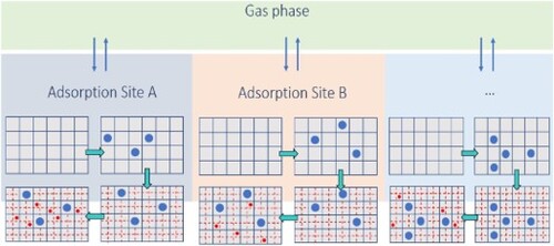
Swisher et al. [22] developed a conceptually simpler approach to deal with the issue of segregation. These authors subdivided the adsorbed pore volume into regions where separate competitive adsorption can take place. Each region is considered to be uniform, where there is a separate thermodynamic equilibrium between the gas and the adsorbed phase. IAST is applied to each of these adsorption sites individually. Therefore, an iterative process is required to calculate the equilibrium loadings at each site. The total adsorbed loadings for the individual components are obtained from the sum of the loadings at each site. This approach is known as the Segregated Ideal Adsorbed Solution theory (SIAST) [22]. This method outperforms IAST when the adsorbent is composed of distinct adsorption sites. The adsorbed loadings estimated using SIAST are in excellent agreement with GCMC data [22] for adsorbents with segregated adsorption sites.

The IAST, RAST and SIAST models involve a set of implicit equations which needs to be solved iteratively. No analytic solution is available for IAST, except for binary mixtures with equal saturation loading [30]. Therefore, these methods are relatively slow from a computational point of view. Instead of IAST or SIAST, the use of an analytic method is computationally much more efficient, especially when incorporated into a breakthrough curve or a reactor model. Explicit isotherms such as mixed Langmuir, mixed Langmuir-Freundlich, etc., are commonly used to compute the adsorption isotherms of components in a mixture. However, these isotherms may not provide correct results for high loadings (low temperature or high pressure) [31]. One of the key assumptions of the mixed Langmuir isotherm is that the adsorbed molecules are not affected by the presence of the other co-adsorbed molecules [32]. The mixed Langmuir equation is thermodynamically inconsistent if the saturation loadings of all components are not equal [33].

Van Assche et al. [34] developed an explicit multi-component adsorption model which accounts for the size effects of the components. In this article, this model will be referred to as Explicit Isotherm (EI). The equations are derived based on the fundamentals of statistical mechanics. The derivation is similar to that of the Langmuir isotherm using statistical mechanics [32]. The adsorbent is considered as a lattice of identical adsorption sites where the component with the smallest saturation capacity (i.e. the largest component) is considered to adsorb first. The remaining sites in the lattice are again uniformly subdivided for the component with the next smallest saturation capacity. This process continues until the adsorption of all components is considered. These authors calculate the expressions for the number of possible ways to perform these arrangements and relate these expressions to the chemical potentials of the components, from which a new set of multi-component explicit isotherms are generated. The model can be extended to any number of components and is capable of capturing the Adsorption Preference Reversal (APR) [35, 36]. This means that at low pressures, it favours the adsorption of components with the largest size or the smallest saturation loading and at high pressures, components with smaller size or larger saturation capacity are preferred [35–38]. This phenomenon is known as size entropy [35, 37]. The model reduces to the single-site Langmuir model for the case of pure components. If the saturation capacities of the components are identical, the model transforms into the mixed Langmuir model. Similar to IAST, this model also assumes uniform adsorption sites. Therefore, it cannot be directly used for the cases where the adsorbent is composed of distinct adsorption sites and the adsorbent exhibits strong segregation effects.

The goal of this work is to extend the EI model to capture the effects of the surface non-uniformity, which is also suggested by Van Assche et al. [34], validate this for different systems, and check for its influence on the breakthrough curve simulations. We have adopted the approach of Swisher et al. [22] to arrive at an explicit adsorption model for realistic segregated adsorption. The adsorbent is subdivided into distinct adsorption sites. Each site is considered to be uniform. The adsorbed phases in these sites are separately in thermodynamic equilibrium with the gas phase. Instead of applying IAST to these sites, we use the explicit isotherms developed by Van Assche et al. [34]. The sum of the adsorbed loadings at each site yields the overall adsorption of the components in the mixture. We will refer to this model as the Segregated Explicit Isotherm (SEI). A comparative study is performed between the SEI, SIAST, IAST models, and GCMC mixture simulations. It is observed that SEI produces results similar to SIAST. Both SEI and SIAST outperform IAST when strong segregation of adsorption sites is prevalent. The values obtained using SEI and SIAST are consistent with GCMC data.

Most industrial separations take place at dynamic conditions [39]. Fixed-bed adsorption is one of the ways to separate components present in a mixture [32]. Breakthrough curve modelling is used to design and analyse such systems [33]. The calculation of equilibrium loadings is an integral part of the breakthrough curve simulations. Although mixed Langmuir isotherms often provide inaccurate equilibrium loadings, especially at high pressures, these isotherms are commonly used to calculate the equilibrium loadings in breakthrough curve simulations [33, 40]. Van Assche et al. [33] have recently implemented the EI model in a process simulation of a Temperature Swing Adsorption (TSA) system for the separation of a 10 component mixture. These authors are able to generate the breakthrough curves about 2.6 times faster than using IAST. In this study, we incorporate SIAST and SEI into a breakthrough curve model and compare their performance with IAST. This comparison is important because using multi-site adsorption isotherms for pure components leads to much slower IAST calculations. IAST involves two iterative processes: (1) calculation of spreading pressure and (2) calculation of the pure component pressure which makes the calculations slow for multi-site adsorption. This will be explained in details in the subsequent sections. As SEI is an explicit model, it will significantly speed up these calculations compared to both SIAST and IAST.

This article is organised as follows: the theory and derivations of different models (SIAST, EI and SEI) are provided in the Section 2. The simulation details are discussed in the Section 3. In the Section 4, we compare the adsorption isotherms obtained using IAST, SIAST, and SEI, and validate these isotherms with GCMC mixture simulations. We also analyse the breakthrough curves computed using these three approaches. In Section 5, we provide conclusions on the results obtained using IAST, SIAST, and SEI.

2. Theory

In this section, we discuss the theory behind the implementation of SIAST and the size-dependent explicit isotherm (EI). We explain the implementation of the segregated approach to the size-dependent explicit isotherm (SEI) and the breakthrough curve modelling approach which is used to compare the effects of IAST, SIAST, and SEI for dynamic conditions.

2.1. Segregated ideal adsorbed solution theory (SIAST)

Instead of considering the available adsorption volume as a continuous space, the adsorbent material is divided into several distinct adsorption sites. The competitive adsorption at each site takes place separately. These sites can be either uniform or heterogeneous. Swisher et al. [22] have considered uniformity for each adsorption site. Each site is separately in thermodynamic equilibrium with the gas phase, as shown in Figure 1. Since the sites are assumed to be uniform, IAST is applied individually to each site. The implementation of this approach is explained below. For a detailed derivation of the IAST, the reader is referred to Refs. [11, 41] Consider a mixture with $N_{\mathrm{c}}$ components. A multi-site Langmuir isotherm which is composed of several single-site Langmuir isotherms is used to calculate the overall adsorbed loadings for the pure components. At each site, one of these single-site Langmuir isotherms is used to calculate the adsorbed loadings of the pure components. For the ith component at the jth site, the adsorption isotherm is (1) $q_{i,j}=q_{\max ,i,j}\frac{k_{i,j}p}{1+k_{i,j}p}$(1) where $q_{i,j}$ is the adsorbed loading and $q_{\max ,i,j}$ is the saturation loading of the component i. The units of both $q_{i,j}$ and $q_{\max ,i,j}$ can be either $[\mathrm{mol}/(\mathrm{kg}\mathrm{framework})]$ or $[\mathrm{molecules}/(\mathrm{unit}\mathrm{cell})]$. $k_{i,j}$ is the equilibrium constant in units of $[1/\mathrm{Pa}]$, and p is the pressure. This constant contains all guest-host interactions including electrostatic interactions. The parameters $(q_{\max ,i,j}\mathrm{and}{k}_{i,j})$ are estimated by fitting the multi-site Langmuir isotherm to the equilibrium loading data obtained using experiments or GCMC simulations. The correspondence between the adsorption sites and the isotherm parameters can be identified using snapshots of molecules present inside the adsorbents, which are obtained using GCMC simulations. In case of only one type of adsorption site, SIAST simply transforms into IAST. In the presence of multiple adsorption sites, adsorption isotherms often show inflection behaviour [42–44]. Inflection behaviour can be observed during the adsorption of branched alkanes inside MFI-type zeolite [42]. This zeolite consists of straight and zigzag channels, and intersections connecting these channels. Branched alkanes preferentially adsorb at the intersections [42]. It is energetically demanding for these molecules to adsorb inside the channels (possible only at high pressure), which is due to the presence of branches [42]. When a mixture includes such components with strong affinity for certain adsorption sites, models with segregated approach like SIAST should be implemented to study adsorption.

Figure 1. Equilibrium of each of the adsorbed phases with the gas phase in the Segregated Ideal Adsorbed Solution Theory (SIAST) model [22]. Each adsorbed phase is separately in equilibrium with the gas phase. The system is at a constant temperature. The gas phase has a total pressure of $p_{\mathrm{tot}}$ and the mole fraction of component i equals $y_i$. In the adsorbed phase j, the loading of component i is $q_{i,j}$.

IAST and SIAST involve the calculation of the spreading pressure $(\pi )$ for each component of the mixture. It is the analogous to pressure but in two dimension [41]. The spreading pressure (π) of the ith component at the jth site is calculated as follows [41] (2) ${\pi }_{i,j}=\frac{RT}{A}{\int }_0^{p_{\mathrm{pure},i,j}}\frac{q_{\mathrm{pure},i,j}(p)}{p}\mathrm{d}p$(2) where $q_{\mathrm{pure},i,j}(p)$ is the adsorbed loading of the pure component. p is the pressure and the upper limit of the integral, $p_{\mathrm{pure},i,j}$ is the pressure of the pure component in the gas phase required to reach the spreading pressure, ${\pi }_{i,j}$. R, T, and A are the absolute temperature, universal gas constant, and surface area, respectively. It is convenient to work with surface potential $(\mathrm{\Psi })$ which is defined as (3) ${\mathrm{\Psi }}_{i,j}=\frac{{\pi }_{i,j}A}{RT}$(3) In Equation  (2(2) ${\pi }_{i,j}=\frac{RT}{A}{\int }_0^{p_{\mathrm{pure},i,j}}\frac{q_{\mathrm{pure},i,j}(p)}{p}\mathrm{d}p$(2) ), we substitute ${\pi }_{i,j}$ with ${\mathrm{\Psi }}_{i,j}$ using Equation  (3(3) ${\mathrm{\Psi }}_{i,j}=\frac{{\pi }_{i,j}A}{RT}$(3) ) and replace $q_{\mathrm{pure},i,j}$ using Equation  (1(1) $q_{i,j}=q_{\max ,i,j}\frac{k_{i,j}p}{1+k_{i,j}p}$(1) ). This leads to (4) ${\mathrm{\Psi }}_{i,j}=q_{\max ,i,j}\ln (1+k_{i,j}{p}_{\mathrm{pure},i,j})$(4) According to IAST, the surface potential of the mixture $({\mathrm{\Psi }}_{\mathrm{mix}})$ is equal to the individual surface potential of the pure components. (5) ${\mathrm{\Psi }}_{{\mathrm{mix},}_j}={\mathrm{\Psi }}_{1,j}={\mathrm{\Psi }}_{2,j}=\cdots ={\mathrm{\Psi }}_{N_{\mathrm{c}},j}$(5) Next, we apply Raoult's law analogy to each adsorption site, which yields (6) $p_i=x_{i,j}{p}_{\mathrm{pure},i,j}\left({\mathrm{\Psi }}_{i,j}\right)$(6) In Equation  (6(6) $p_i=x_{i,j}{p}_{\mathrm{pure},i,j}\left({\mathrm{\Psi }}_{i,j}\right)$(6) ), $p_i$ is the partial pressure of component i in the gas phase and $x_{i,j}$ is the mole fraction of component i in the adsorbed phase. At each site j, an independent mass balance is applicable for $N_{\mathrm{c}}$ number of components. (7) $\sum _{i=1}^{N_{\mathrm{c}}}{x}_{i,j}=1$(7) Since the pure component pressures, $p_{\mathrm{pure},i,j}$ cannot be calculated apriori, ${\mathrm{\Psi }}_{i,j}$ in Equation (4(4) ${\mathrm{\Psi }}_{i,j}=q_{\max ,i,j}\ln (1+k_{i,j}{p}_{\mathrm{pure},i,j})$(4) ) is obtained using iterative schemes such as the Newton-Raphson [45] and the bisection method [45]. The bisection method is used in this work as it can generate values correct up to machine precision, which is not possible in practice with the Newton-Raphson method. Moreover, the Newton-Raphson method is highly sensitive to the initial conditions, and eventually the algorithm can easily lead to divergence of the solution. The magnitude of $x_{i,j}$ is calculated using the inverse of Equation  (4(4) ${\mathrm{\Psi }}_{i,j}=q_{\max ,i,j}\ln (1+k_{i,j}{p}_{\mathrm{pure},i,j})$(4) ). In this equation, $p_{\mathrm{pure},i,j}$ is substituted using Equation  (6(6) $p_i=x_{i,j}{p}_{\mathrm{pure},i,j}\left({\mathrm{\Psi }}_{i,j}\right)$(6) ). If the analytic inversion of the surface potential (the inverse of Equation  (4(4) ${\mathrm{\Psi }}_{i,j}=q_{\max ,i,j}\ln (1+k_{i,j}{p}_{\mathrm{pure},i,j})$(4) )) does not provide an explicit expression at each adsorption site, then SIAST will not perform better than IAST.

The total loading on the jth site equals [41] (8) $q_{\mathrm{tot},j}={\left[\sum _{i=1}^{N_{\mathrm{c}}}\frac{x_{i,j}}{q_{\mathrm{pure},i,j}}\right]}^{-1}$(8) The loading of component i is calculated as follows (9) $q_{i,j}=x_{i,j}{q}_{\mathrm{tot},j}$(9) The total loading for the ith component $(q_i)$ encompassing all the sites is (10) $q_i=\sum _{j=1}^{N_{\mathrm{sites}}}{q}_{i,j}$(10)

2.2. Explicit isotherm (EI)

The explicit isotherm model developed by Van Assche et al. [34] considers the adsorbent as a uniform lattice subdivided into identical adsorption sites. These adsorption sites can accommodate the largest species present in the mixture. First, we will derive the equations for a binary mixture. Consider that species 1 is the largest species. The lattice is divided into $M_1$ sites for the adsorption of species 1. The number of ways to adsorb N indistinguishable molecules of species 1 is: (11) $\frac{\left(M_1\right)!}{(M_1-N)!N!}$(11) Figure 2(a,b) show the adsorption of N indistinguishable molecules of species 1 on an adsorbent which is subdivided into $M_1$ uniform lattice sites. Next, species 2 will be adsorbed in the lattice. Species 2 is the smaller of the two components. It is considered to be n times smaller than species 1. After adsorption of species 1, the remaining sites in the lattice $(M_1-N)$ are further subdivided. Each site is now divided into n parts. Therefore, $(n{M}_1-nN)$ sites are available for the adsorption of species 2 Figure 2(c). We rewrite $n{M}_1$ as M which is the total number of available sites for adsorption of species 2 in the absence of species 1. K molecules of species 2 are adsorbed on the remaining sites which is shown in Figure 2(d). The number of ways for this arrangement, considering the indistinguishable nature of the molecules, is (12) $\frac{(M-nN)!}{(M-nN-K)!K!}$(12) The canonical partition function Z for this mixture can be written as [34] (13) $Z=\frac{M_1!}{(M_1-N)!N!}\frac{(M-nN)!}{(M-nN-K)!K!}{f}_1^N{f}_2^K$(13) where, $f_1$ and $f_2$ are the molecular partition functions for individually adsorbed molecules. The relation between the canonical function and the partial pressures of the components are [32, 34]. (14) $\begin{array}{rl}\frac{{\mu }_1}{k_{\mathrm{B}}T}& =\frac{{\mu }_1^0}{k_{\mathrm{B}}T}+\ln \left(\frac{p_1}{p^0}\right)=-{\left(\frac{\mathrm{\partial }\ln (Z)}{\mathrm{\partial }N}\right)}_{K,M,T}\end{array}$(14) (15) $\begin{array}{rl}\frac{{\mu }_2}{k_{\mathrm{B}}T}& =\frac{{\mu }_2^0}{k_{\mathrm{B}}T}+\ln \left(\frac{p_2}{p^0}\right)=-{\left(\frac{\mathrm{\partial }\ln (Z)}{\mathrm{\partial }K}\right)}_{N,M,T}\end{array}$(15) where, ${\mu }_i^0$ is the chemical potential of component i in the pure form at pressure $(p^0)$. The reference pressure, $p^0$ is considered to be 1 bar. $p_i$ is the partial pressure of component i in the mixture. To introduce the equilibrium constants $(k_i)$ for the adsorption of the pure components 1 and 2 in Equations  (14(14) $\begin{array}{rl}\frac{{\mu }_1}{k_{\mathrm{B}}T}& =\frac{{\mu }_1^0}{k_{\mathrm{B}}T}+\ln \left(\frac{p_1}{p^0}\right)=-{\left(\frac{\mathrm{\partial }\ln (Z)}{\mathrm{\partial }N}\right)}_{K,M,T}\end{array}$(14) ) and (15(15) $\begin{array}{rl}\frac{{\mu }_2}{k_{\mathrm{B}}T}& =\frac{{\mu }_2^0}{k_{\mathrm{B}}T}+\ln \left(\frac{p_2}{p^0}\right)=-{\left(\frac{\mathrm{\partial }\ln (Z)}{\mathrm{\partial }K}\right)}_{N,M,T}\end{array}$(15) ), we use the following equations (16) $\begin{array}{rl}{k}_1& =f_1(T)\exp \left(\frac{{\mu }_1^0}{k_{\mathrm{B}}T}\right)\end{array}$(16) (17) $\begin{array}{rl}{k}_2& =f_2(T)\exp \left(\frac{{\mu }_2^0}{k_{\mathrm{B}}T}\right)\end{array}$(17) We substitute the canonical function Z in Equations  (14(14) $\begin{array}{rl}\frac{{\mu }_1}{k_{\mathrm{B}}T}& =\frac{{\mu }_1^0}{k_{\mathrm{B}}T}+\ln \left(\frac{p_1}{p^0}\right)=-{\left(\frac{\mathrm{\partial }\ln (Z)}{\mathrm{\partial }N}\right)}_{K,M,T}\end{array}$(14) ) and (15(15) $\begin{array}{rl}\frac{{\mu }_2}{k_{\mathrm{B}}T}& =\frac{{\mu }_2^0}{k_{\mathrm{B}}T}+\ln \left(\frac{p_2}{p^0}\right)=-{\left(\frac{\mathrm{\partial }\ln (Z)}{\mathrm{\partial }K}\right)}_{N,M,T}\end{array}$(15) ) using Equation  (13(13) $Z=\frac{M_1!}{(M_1-N)!N!}\frac{(M-nN)!}{(M-nN-K)!K!}{f}_1^N{f}_2^K$(13) ). These equations are further modified by substituting ${\mu }_i^0$ using Equations  (16(16) $\begin{array}{rl}{k}_1& =f_1(T)\exp \left(\frac{{\mu }_1^0}{k_{\mathrm{B}}T}\right)\end{array}$(16) ) and (17(17) $\begin{array}{rl}{k}_2& =f_2(T)\exp \left(\frac{{\mu }_2^0}{k_{\mathrm{B}}T}\right)\end{array}$(17) ) and applying Stirling's approximation to the right-hand side of the equations [34]. The reader is referred to the Supporting Information of Ref. [34] for a detailed derivation. The fractional loadings $(q_i/q_{\max ,i,j})$ of the components are defined as ${\theta }_1=nN/M$ and ${\theta }_2=K/M$. Using Equations (14(14) $\begin{array}{rl}\frac{{\mu }_1}{k_{\mathrm{B}}T}& =\frac{{\mu }_1^0}{k_{\mathrm{B}}T}+\ln \left(\frac{p_1}{p^0}\right)=-{\left(\frac{\mathrm{\partial }\ln (Z)}{\mathrm{\partial }N}\right)}_{K,M,T}\end{array}$(14) )– (17(17) $\begin{array}{rl}{k}_2& =f_2(T)\exp \left(\frac{{\mu }_2^0}{k_{\mathrm{B}}T}\right)\end{array}$(17) ), we obtain the following equations for the isotherms: (18) $\begin{array}{rl}{k}_1{p}_1& =\frac{{\theta }_1{(1-{\theta }_1)}^{n-1}}{{(1-{\theta }_1-{\theta }_2)}^n}\end{array}$(18) (19) $\begin{array}{rl}{k}_2{p}_2& =\frac{{\theta }_2}{(1-{\theta }_1-{\theta }_2)}\end{array}$(19) Equations  (18(18) $\begin{array}{rl}{k}_1{p}_1& =\frac{{\theta }_1{(1-{\theta }_1)}^{n-1}}{{(1-{\theta }_1-{\theta }_2)}^n}\end{array}$(18) ) and (19(19) $\begin{array}{rl}{k}_2{p}_2& =\frac{{\theta }_2}{(1-{\theta }_1-{\theta }_2)}\end{array}$(19) ) are the implicit forms of the isotherm model. Rearranging these equations leads to the set of explicit binary adsorption isotherms (20) $\begin{array}{rl}{q}_1& =q_{\max ,1}\frac{k_1{p}_1}{{(1+k_2{p}_2)}^n+k_1{p}_1}\end{array}$(20) (21) $\begin{array}{rl}{q}_2& =q_{\max ,2}\frac{k_2{p}_2{(1+k_2{p}_2)}^{n-1}}{{(1+k_2{p}_2)}^n+k_1{p}_1}\end{array}$(21) This model can be extended to an arbitrary number of components $(N_{\mathrm{c}})$. The following condition is imposed for the saturation capacities: (22) $q_{\max ,N_{\mathrm{c}}}\ge q_{\max ,N_{\mathrm{c}}-1}\ge \cdots \ge q_{\max ,2}\ge q_{\max ,1}$(22) Following a similar derivation, for a mixture of $N_{\mathrm{c}}$ components, the isotherm for the ith component is as follows [34] (23) $q_i=\left(q_{\max ,1}{k}_i{p}_i\right)\frac{\left[\prod _{m=1}^i{\alpha }_m\right]}{\beta }$(23) where, (24) $\begin{array}{rl}{\alpha }_1& =1\end{array}$(24) (25) $\begin{array}{rl}{\alpha }_i& =[(\cdots (({(1+k_{N_{\mathrm{c}}}{p}_{N_{\mathrm{c}}})}^{n_{N_{\mathrm{c}}}}\\ & {{+k_{N_{\mathrm{c}}-1}{p}_{N_{\mathrm{c}}-1})}^{n_{N_{\mathrm{c}}-1}}+k_{N_{\mathrm{c}}-2}{p}_{N_{\mathrm{c}}-2})}^{n_{N_{\mathrm{c}}-2}}\dots \\ & {{+k_{i+1}{p}_{i+1})}^{n_{i+1}}+k_i{p}_i]}^{n_i-1}\end{array}$(25) (26) $\begin{array}{rl}\beta & =[(\cdots (({(1+k_N{p}_{N_{\mathrm{c}}})}^{n_{N_{\mathrm{c}}}}\\ & {{+k_{N_{\mathrm{c}}-1}{p}_{N_{\mathrm{c}}-1})}^{n_{N_{\mathrm{c}}-1}}+k_{N_{\mathrm{c}}-2}{p}_{N_{\mathrm{c}}-2})}^{n_{N_{\mathrm{c}}-2}}\dots \\ & {+k_2{p}_2)}^{n_2}+k_1{p}_1]\end{array}$(26) In Equations  (25(25) $\begin{array}{rl}{\alpha }_i& =[(\cdots (({(1+k_{N_{\mathrm{c}}}{p}_{N_{\mathrm{c}}})}^{n_{N_{\mathrm{c}}}}\\ & {{+k_{N_{\mathrm{c}}-1}{p}_{N_{\mathrm{c}}-1})}^{n_{N_{\mathrm{c}}-1}}+k_{N_{\mathrm{c}}-2}{p}_{N_{\mathrm{c}}-2})}^{n_{N_{\mathrm{c}}-2}}\dots \\ & {{+k_{i+1}{p}_{i+1})}^{n_{i+1}}+k_i{p}_i]}^{n_i-1}\end{array}$(25) ) and (26(26) $\begin{array}{rl}\beta & =[(\cdots (({(1+k_N{p}_{N_{\mathrm{c}}})}^{n_{N_{\mathrm{c}}}}\\ & {{+k_{N_{\mathrm{c}}-1}{p}_{N_{\mathrm{c}}-1})}^{n_{N_{\mathrm{c}}-1}}+k_{N_{\mathrm{c}}-2}{p}_{N_{\mathrm{c}}-2})}^{n_{N_{\mathrm{c}}-2}}\dots \\ & {+k_2{p}_2)}^{n_2}+k_1{p}_1]\end{array}$(26) ), the value of $n_i$ for component i is $q_{\max ,i}/q_{\max ,i-1}$.

2.3. Segregated explicit isotherm (SEI)

Similar to SIAST, we also consider the equilibrium of each adsorption site separately with the gas phase, as shown in Figure 3. The isotherms derived in section (Explicit Isotherm) are solved separately for adsorption site j. (27) $q_{i,j}=\left(q_{\max ,i,j}{k}_{i,j}{p}_i\right)\frac{\left[\prod _{m=1}^i{\alpha }_{m,j}\right]}{{\beta }_j}$(27) The overall loading $(q_i)$ for component i is obtained by summing over the loadings for the component calculated at each adsorption site. (28) $q_i=\sum _{j=1}^{N_{\mathrm{sites}}}{q}_{i,j}$(28) In Equation  (28(28) $q_i=\sum _{j=1}^{N_{\mathrm{sites}}}{q}_{i,j}$(28) ), $N_{\mathrm{sites}}$ is the number of sites available for adsorption, which is the same for all components. The procedure for calculating the equilibrium loadings using SEI is shown in Algorithm 1. In this algorithm, Equations  (23(23) $q_i=\left(q_{\max ,1}{k}_i{p}_i\right)\frac{\left[\prod _{m=1}^i{\alpha }_m\right]}{\beta }$(23) )–(26(26) $\begin{array}{rl}\beta & =[(\cdots (({(1+k_N{p}_{N_{\mathrm{c}}})}^{n_{N_{\mathrm{c}}}}\\ & {{+k_{N_{\mathrm{c}}-1}{p}_{N_{\mathrm{c}}-1})}^{n_{N_{\mathrm{c}}-1}}+k_{N_{\mathrm{c}}-2}{p}_{N_{\mathrm{c}}-2})}^{n_{N_{\mathrm{c}}-2}}\dots \\ & {+k_2{p}_2)}^{n_2}+k_1{p}_1]\end{array}$(26) ) are shown in a recursive manner.

2.4. Breakthrough curve model

Breakthrough curves reflect the concentration profiles of the components in a mixture at the outlet of the fixed bed adsorption column [46]. Modelling breakthrough curves involves the mass balance for different species present in the mixture. We write the mass transport equation for each component in terms of their partial pressures in the gas phase $(p_i)$. We assume the ideal gas law to be valid. Considering plug flow and isothermal conditions and neglecting axial dispersion, we obtain the following equation for mass transport [18, 47]. (29) $\begin{array}{rl}\frac{\mathrm{\partial }{p}_i(t,z)}{\mathrm{\partial }t}& =-\frac{\mathrm{\partial }\left(v(t,z)p_i(t,z)\right)}{\mathrm{\partial }z}\\ & -RT\left(\frac{1-{\epsilon }_{\mathrm{b}}}{{\epsilon }_{\mathrm{b}}}\right){\rho }_{\mathrm{p}}\frac{\mathrm{\partial }{q}_i(t,z)}{\mathrm{\partial }t}\end{array}$(29) In Equation  (29(29) $\begin{array}{rl}\frac{\mathrm{\partial }{p}_i(t,z)}{\mathrm{\partial }t}& =-\frac{\mathrm{\partial }\left(v(t,z)p_i(t,z)\right)}{\mathrm{\partial }z}\\ & -RT\left(\frac{1-{\epsilon }_{\mathrm{b}}}{{\epsilon }_{\mathrm{b}}}\right){\rho }_{\mathrm{p}}\frac{\mathrm{\partial }{q}_i(t,z)}{\mathrm{\partial }t}\end{array}$(29) ), $p_i$ is the partial pressure of component i in the gas phase in $[\mathrm{Pa}]$, v is the interstitial velocity in $[\mathrm{m}/\mathrm{s}]$. The fixed bed void fraction is defined by ${\epsilon }_{\mathrm{b}}$, ${\rho }_{\mathrm{p}}$ is the adsorbent material density in $[\mathrm{kg}/{\mathrm{m}}^3]$, and z is the position along the column. The interstitial velocity is calculated using the total mass balance. We write the total mass balance in terms of the total pressure $(p_{\mathrm{tot}})$ and impose isobaric conditions in the column [48]. (30) $\frac{\mathrm{\partial }\left(v(t,z)\right)}{\mathrm{\partial }z}=-\frac{RT}{p_{\mathrm{tot}}}\left(\frac{1-{\epsilon }_{\mathrm{b}}}{{\epsilon }_{\mathrm{b}}}\right){\rho }_{\mathrm{p}}\sum _{i=1}^{N_{\mathrm{c}}}\frac{\mathrm{\partial }{q}_i(t,z)}{\mathrm{\partial }t}$(30) The term $\frac{\mathrm{\partial }{q}_i(t,z)}{\mathrm{\partial }t}$ in Equations  (29(29) $\begin{array}{rl}\frac{\mathrm{\partial }{p}_i(t,z)}{\mathrm{\partial }t}& =-\frac{\mathrm{\partial }\left(v(t,z)p_i(t,z)\right)}{\mathrm{\partial }z}\\ & -RT\left(\frac{1-{\epsilon }_{\mathrm{b}}}{{\epsilon }_{\mathrm{b}}}\right){\rho }_{\mathrm{p}}\frac{\mathrm{\partial }{q}_i(t,z)}{\mathrm{\partial }t}\end{array}$(29) ) and (30(30) $\frac{\mathrm{\partial }\left(v(t,z)\right)}{\mathrm{\partial }z}=-\frac{RT}{p_{\mathrm{tot}}}\left(\frac{1-{\epsilon }_{\mathrm{b}}}{{\epsilon }_{\mathrm{b}}}\right){\rho }_{\mathrm{p}}\sum _{i=1}^{N_{\mathrm{c}}}\frac{\mathrm{\partial }{q}_i(t,z)}{\mathrm{\partial }t}$(30) ) accounts for the mass transfer of the species from the gas phase to the adsorbed phase. It is often modelled using the Linear Driving Force model (LDF) [49] (31) $\frac{\mathrm{\partial }{q}_i(t,z)}{\mathrm{\partial }t}=k_{\mathrm{M},i}(q_{\mathrm{eq},i}-q_i)$(31) The LDF model states that the rate of adsorption is proportional to the amount of adsorbate still required to achieve equilibrium between the gas and the adsorbed phase [50]. In Equation  (31(31) $\frac{\mathrm{\partial }{q}_i(t,z)}{\mathrm{\partial }t}=k_{\mathrm{M},i}(q_{\mathrm{eq},i}-q_i)$(31) ), the mass transfer coefficient is defined by $k_{\mathrm{M},i}$ in $[1/\mathrm{s}]$. $q_{\mathrm{eq},i}$ is the equilibrium loading and $q_i$ is the adsorbed loading of component i. The units of $q_{\mathrm{eq},i}$ and $q_i$ are in $[\mathrm{mol}/(\mathrm{kgframework})]$. To calculate the magnitude of $q_{\mathrm{eq},i}$, an adsorption model must be integrated with the breakthrough curve model. We incorporated both SIAST and SEI into the breakthrough model and made a detailed comparison in terms of accuracy and computational requirements.

Figure 2. Representation of the adsorbent as a lattice where species of different sizes are adsorbed [34]. (a) The adsorbent is divided into $M_1$ sites. (b) adsorption of N indistinguishable molecules of species 1, represented by the blue circles, is taking place on the lattice. (c) After the adsorption of N molecules of species 1, the remaining lattice sites are further divided into $(n{M}_1-nN)$ sites. (d) adsorption of K indistinguishable molecules of species 2 is taking place on the lattice. The blue circles represent species 1 and the smaller red circles represent species 2.

Figure 3. Representation of Segregated Explicit Isotherm (SEI) model which accounts for the separate thermodynamic equilibria of the adsorbed phases with the gas phase at different adsorption sites. Each adsorbed phase is separately in thermodynamic equilibrium with the gas phase and it is represented by the adsorption isotherm proposed by Van Assche et al. [34] Equation (23(23) $q_i=\left(q_{\max ,1}{k}_i{p}_i\right)\frac{\left[\prod _{m=1}^i{\alpha }_m\right]}{\beta }$(23) ). The gas phase has a total pressure of $p_{\mathrm{tot}}$ and the gas phase mole fractions of the components in the mixture are represented by $y_i$. In the adsorbed phase j, the loading of the component i is $q_{i,j}$.

3. Simulation details

We consider two case studies of adsorption of binary equimolar (50:50) mixtures:

1. carbon dioxide $({\mathrm{CO}}_2)$ and propane $({\mathrm{C}}_3)$ on MOR-type zeolite at 300K [22].

2. butane $({\mathrm{nC}}_4)$ and 2-methyl propane$({2\mathrm{mC}}_3)$ on MFI-type zeolite at 400K.

To calculate the mixture isotherms, we first need to generate the pure component isotherms. Adsorption loadings for the pure components are calculated using GCMC simulations [8] which are performed using the RASPA software [51, 52]. The non-bonded intermolecular interactions (both guest-guest and guest-host) are modelled by Lennard-Jones potentials and electrostatic interactions. The latter are computed using the Ewald summation [53]. The Lennard-Jones parameters and the partial charges are obtained from various sources. For ${\mathrm{CO}}_2$, these parameters are taken from the work of Garcia-Sanchez et al. [54]. The force field of Dubbeldam et al. [55]. is used for the ${\mathrm{C}}_3$, ${\mathrm{nC}}_4$, and ${2\mathrm{mC}}_3$ molecules. Interactions between sorbent atoms of different type are taking into account via the Lorentz-Berthelot mixing rules. To account for the interaction between the adsorbed molecules and the adsorbent, the TraPPE-zeo force field is used [56]. Both the zeolites (MOR-type and MFI-type) are pure silicalites and do not contain any extra-framework cations. Short range interactions were truncated and shifted to zero at 12 $\text{Å}$. ${\mathrm{CO}}_2$ is considered a rigid molecule, so the bonded interactions are not considered. The bonded interactions for the hydrocarbons are modelled using the united atom TraPPE force fields [57]. In the first study, the simulation box consists of 16 unit cells $(2\times 2\times 4)$, and 8 unit cells $(2\times 2\times 2)$ in the second case. Ideal gas behaviour is assumed for the gas phase. For a pure component in the gas phase, the fugacity is equal to the pressure of the pure component (p). For mixtures, the fugacity of component i is equal to the total pressure multiplied by the gas phase mole fraction $(y_i)$.

The error bars present in the GCMC simulation data are significantly less than ca. $2\mathrm{\%}$. The datasets are fitted to the multi-site Langmuir isotherms to obtain the isotherm parameters, saturation loadings $(q_{\max ,i,j})$ and equilibrium constants $(k_{i,j})$. To obtain the correct loadings, it is crucial to identify which isotherm parameters correspond to which adsorption site. This is because the preference for the adsorption sites for different components in the mixture may vary. A molecule of an adsorbed species will experience the competition only from those molecules of the other species which are adsorbed at the same site. The correspondence between the adsorption sites and the isotherm parameters is identified using simulation snapshots. The data sets for the snapshots are generated during the GCMC simulations performed with the RASPA software [51, 52]. The iRASPA software is used to create the images using these data sets [58].

$q_{\max ,i,j}$, $k_{i,j}$ and the partial pressures $(p_i)$ of the components in the gas phase are the main input parameters for the mixture isotherm models. The mixture isotherms are computed using IAST, SIAST and SEI. In IAST and SIAST, the system of implicit equations is solved using the bisection method [45] which enables us to compute the equilibrium loadings correct up to machine precision. This is essential when IAST or SIAST is incorporated into breakthrough curve models. A small difference in the equilibrium loading can lead to a breakthrough curve quite different from the actual curve, so therefore it is advised to solve the IAST equations as accurate as possible. For the purpose of validation, we have also calculated the adsorbed loadings for the mixtures using GCMC simulations. Comparisons are made between the adsorption isotherms generated using these four methods.

For the breakthrough curve modelling, Equations  (29(29) $\begin{array}{rl}\frac{\mathrm{\partial }{p}_i(t,z)}{\mathrm{\partial }t}& =-\frac{\mathrm{\partial }\left(v(t,z)p_i(t,z)\right)}{\mathrm{\partial }z}\\ & -RT\left(\frac{1-{\epsilon }_{\mathrm{b}}}{{\epsilon }_{\mathrm{b}}}\right){\rho }_{\mathrm{p}}\frac{\mathrm{\partial }{q}_i(t,z)}{\mathrm{\partial }t}\end{array}$(29) )– (31(31) $\frac{\mathrm{\partial }{q}_i(t,z)}{\mathrm{\partial }t}=k_{\mathrm{M},i}(q_{\mathrm{eq},i}-q_i)$(31) ) are solved simultaneously. Initially, the column is filled with only a non-adsorbing carrier gas (helium). At the start of the breakthrough simulation, the pressure of the carrier gas is equal to the total pressure inside the column $(p_{\mathrm{carrier}\mathrm{gas}}=p_{\mathrm{tot}})$. The adsorber column is considered to be isothermal and isobaric. The initial conditions are: (32) $\begin{array}{rl}v(t=0,z)& =v_{\mathrm{in}}\end{array}$(32) (33) $\begin{array}{rl}{p}_{\mathrm{tot}}(t=0,z)& =p_{\mathrm{tot},\mathrm{in}}\end{array}$(33) (34) $\begin{array}{rl}{p}_{\mathrm{carrier}\mathrm{gas}}(t=0,z)& =p_{\mathrm{tot}}(t=0,z)\end{array}$(34) (35) $\begin{array}{rl}{p}_i(t=0,z>0)& =0\end{array}$(35) (36) $\begin{array}{rl}{q}_i(t=0,z)& =0\end{array}$(36) where v is the interstitial velocity and $v_{\mathrm{in}}$ is the interstitial velocity at the inlet of the adsorber. $p_{\mathrm{tot}}$ is the total pressure of the adsorber column and the total pressure at the inlet is referred to as $p_{\mathrm{tot},\mathrm{in}}$. $p_{\mathrm{carrier}\mathrm{gas}}$ is the partial pressure of the carrier gas. $p_i$ and $q_i$ are the partial pressure and adsorbed loadings of the component i, respectively. At the inlet of the column, the partial pressures for each component and the velocity are fixed. At the outlet, the spatial gradients of the partial pressures are considered to be zero. The boundary conditions for the simulations are as follows (37) $\begin{array}{rl}v(t,z=0)& =v_{\mathrm{in}}\end{array}$(37) (38) $\begin{array}{rl}{p}_{\mathrm{tot}}(t,z=0)& =p_{\mathrm{tot},\mathrm{in}}\end{array}$(38) (39) $\begin{array}{rl}{p}_i(t,z=0)& =y_{i,\mathrm{in}}\cdot p_{\mathrm{tot},\mathrm{in}}\end{array}$(39) (40) $\begin{array}{rl}\frac{\mathrm{\partial }{p}_i(t,z=L)}{\mathrm{\partial }z}& =0\end{array}$(40) Equations  (29(29) $\begin{array}{rl}\frac{\mathrm{\partial }{p}_i(t,z)}{\mathrm{\partial }t}& =-\frac{\mathrm{\partial }\left(v(t,z)p_i(t,z)\right)}{\mathrm{\partial }z}\\ & -RT\left(\frac{1-{\epsilon }_{\mathrm{b}}}{{\epsilon }_{\mathrm{b}}}\right){\rho }_{\mathrm{p}}\frac{\mathrm{\partial }{q}_i(t,z)}{\mathrm{\partial }t}\end{array}$(29) )–(31(31) $\frac{\mathrm{\partial }{q}_i(t,z)}{\mathrm{\partial }t}=k_{\mathrm{M},i}(q_{\mathrm{eq},i}-q_i)$(31) ) form a system of differential algebraic equations. The method of lines [59] is used to solve these equations numerically. The spatial derivatives present in the partial differential equations (PDEs) are discretised using the Finite Difference Method (FDM) [60]. The advective terms $(\mathrm{\partial }(v{p}_i)/\mathrm{\partial }z)$ and $(\mathrm{\partial }(v)/\mathrm{\partial }z)$ in Equations  (29(29) $\begin{array}{rl}\frac{\mathrm{\partial }{p}_i(t,z)}{\mathrm{\partial }t}& =-\frac{\mathrm{\partial }\left(v(t,z)p_i(t,z)\right)}{\mathrm{\partial }z}\\ & -RT\left(\frac{1-{\epsilon }_{\mathrm{b}}}{{\epsilon }_{\mathrm{b}}}\right){\rho }_{\mathrm{p}}\frac{\mathrm{\partial }{q}_i(t,z)}{\mathrm{\partial }t}\end{array}$(29) ) and (30(30) $\frac{\mathrm{\partial }\left(v(t,z)\right)}{\mathrm{\partial }z}=-\frac{RT}{p_{\mathrm{tot}}}\left(\frac{1-{\epsilon }_{\mathrm{b}}}{{\epsilon }_{\mathrm{b}}}\right){\rho }_{\mathrm{p}}\sum _{i=1}^{N_{\mathrm{c}}}\frac{\mathrm{\partial }{q}_i(t,z)}{\mathrm{\partial }t}$(30) ), respectively, are discretised using a first-order upwind scheme [61]. The Strong Stability Preserving Runge Kutta (SSP-RK(3,3)) method is used for the time integration [62, 63]. This is a third-order scheme and involves three stages in the integration [64].

The input parameters for the simulations are shown in Table 1 and the mass transfer coefficients for the components of the mixtures are shown in Table 2. The length of the adsorber column for the first case is considered to be 0.1 m and 0.8 m for the second case. The lengths of the columms are discretised with a uniform grid size, $\mathrm{\Delta }z$. For the first case, $\mathrm{\Delta }z$ is 0.005 and 0.05 m for the second case. is chosen as A time step $(\mathrm{\Delta }t=0.001\mathrm{s})$ was chosen for the time integration in both cases.

For the simulations, the following High Performance Computing (HPC) facilities were used: (1) Dutch National Supercomputer (Snellius), and (2) a local supercomputer at Delft University of Technology (HAL9000).

Table 1. Input parameters for the simulation of the breakthrough curve (catalyst particle density, $({\rho }_{\mathrm{p}})$, bed voidage $({\epsilon }_{\mathrm{b}})$, interstitial velocity at the inlet, $(v_{\mathrm{in}})$, and total pressure $(p_{\mathrm{tot}})$) for both cases.

	${\rho }_{\mathrm{p}}[\mathrm{kg}/{\mathrm{m}}^3]$	${\epsilon }_{\mathrm{b}}$	$v_{\mathrm{in}}[\mathrm{m}/\mathrm{s}]$	$p_{\mathrm{tot}}[\mathrm{bar}]$
${\mathrm{CO}}_2-{\mathrm{C}}_3$	1711.06	0.128	0.1	1.0
${\mathrm{nC}}_4-{2\mathrm{mC}}_3$	1796.34	0.40	0.1	10.0

Table 2. Mass transfer coefficients $(k_{\mathrm{M}})$ for the components in both the case studies.

	${\mathrm{CO}}_2$	${\mathrm{C}}_3$	${\mathrm{nC}}_4$	${2\mathrm{mC}}_3$
$k_{\mathrm{m}}[1/\mathrm{s}]$	0.06	0.06	0.06	0.06

4. Results and discussions

In this section, we discuss the adsorption isotherms obtained for pure components and their mixtures in both studies (${\mathrm{CO}}_2$-${\mathrm{C}}_3$ mixture in MOR-type zeolite at 300K, and an ${\mathrm{nC}}_4$-${2\mathrm{mC}}_3$ mixture in MFI-type zeolite at 400K). We compare the results predicted by IAST, SIAST and SEI. For the purpose of validation, mixture isotherm data using GCMC simulations are generated. The influence of the different models (SIAST and SEI) on the breakthrough curves is also investigated.

4.1. Adsorption isotherms

4.1.1. ${\mathrm{CO}}_2$ – ${\mathrm{C}}_3$ mixture, MOR-type Zeolite, 300K

Pure component loadings are calculated using GCMC simulations and fitted to dual-site Langmuir isotherms. This is because there are two possible distinct sites for adsorption inside MOR-type zeolite. The pure component isotherms are shown in Figure 4 and the corresponding fitted parameters are listed in Table 3. In the dual-site Langmuir isotherm, we have two pairs of fitted parameters, which are saturation loading $(q_{\max ,i,j})$ and equilibrium constant $(k_{i,j})$ at each site. The GCMC data generated in this work are in excellent agreement with the data obtained by Swisher et al. [22]. To identify the correspondence between the pairs of fitted parameters and the adsorption sites, we have generated the snapshots of adsorption of the pure components inside the MOR-type zeolite using the iRASPA software [58].

Figure 4. Pure component adsorption isotherms of ${\mathrm{CO}}_2$ and ${\mathrm{C}}_3$ in MOR-type zeolite at 300K. Pure component adsorbed loadings calculated using GCMC for the pressure range $({10}^0-5\cdot {10}^{10})$ Pa are fitted to the dual-site Langmuir isotherms. The empty circles represent GCMC simulation data and the solid lines are the dual-site Langmuir isotherms fitted to these data sets. The results obtained in this work are in excellent agreement with the data published by Swisher et al. [22].

Table 3. Fitted parameters for the adsorption of pure ${\mathrm{CO}}_2$ and ${\mathrm{C}}_3$ in MOR-type zeolite at 300 K.

	$k_1[1/\mathrm{Pa}]$	$q_{\max ,1}[\mathrm{mol}/(\mathrm{kgframework})]$	$k_2[1/\mathrm{Pa}]$	$q_{\max ,2}[\mathrm{mol}/(\mathrm{kgframework})]$
${\mathrm{CO}}_2$	$2.617\cdot {10}^{-4}$	1.60	$4.859\cdot {10}^{-7}$	3.62
${\mathrm{C}}_3$	$6.506\cdot {10}^{-9}$	1.73	$2.376\cdot {10}^{-4}$	1.09

Notes: Adsorbed loadings obtained from the GCMC simulations for the pressure range $({10}^0-5\cdot {10}^{10})$ Pa are fitted using the dual-site Langmuir isotherm. Subscript 1 indicates site 1 (smaller pockets) and subscript 2 indicates site 2 (larger pockets) present inside MOR-type zeolite. (See also Figure 5.).

Figure 5(a,b) show typical snapshots of pure ${\mathrm{CO}}_2$ inside MOR-type at 300K. The snapshots are taken at ${10}^3$Pa and ${10}^9$Pa respectively. Similarly, Figure 5(c,d) show the snapshots for ${\mathrm{C}}_3$ molecules at conditions (temperature and pressure) identical to the case of ${\mathrm{CO}}_2$. At low pressure, ${\mathrm{CO}}_2$ preferentially adsorbs inside the smaller pockets (site 1) and ${\mathrm{C}}_3$ adsorbs inside the larger ones (site 2). At higher pressures, once the preferred type of site is filled, the molecules start adsorbing on the remaining types of sites. 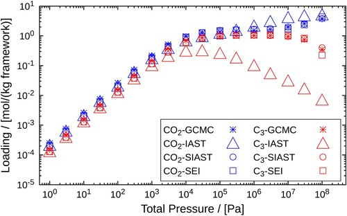Therefore, at higher pressures, both ${\mathrm{CO}}_2$ and ${\mathrm{C}}_3$ are found in both types of adsorbing pockets. This is clearly shown in Figure 5(b,d). For assigning the pairs of fitted parameters to the adsorption sites, we refer to the smaller pockets as site 1 and the larger ones as site 2. The values of these parameters are shown in Table 3. Next, we compare the mixture isotherms predicted by IAST, SIAST, and SEI and validate the predictions by further comparing with the GCMC simulations for the mixture. Figure 6 shows the isotherms for the mixture of ${\mathrm{CO}}_2$ and ${\mathrm{C}}_3$. We can observe the deviations in the adsorption isotherms predicted by the IAST from the GCMC data. The isotherms obtained using SEI and SIAST are in good agreement with the GCMC simulation data. There are very small deviations at higher pressures $(\sim {10}^8\mathrm{Pa})$ from the GCMC calculations for both SEI and SIAST, but these deviations are much lower compared to the IAST predictions.

The deviations can be explained based on the preference for the adsorption sites. IAST underpredicts the adsorbed loadings for ${\mathrm{C}}_3$ molecules and overpredicts for ${\mathrm{CO}}_2$. This is clearly because of the underlying assumption of the presence of uniform adsorbents in the IAST model. This assumption is correct only when the molecules do not have any preference for the adsorption sites. However, in this case, the components clearly favour one site over the other. At higher pressures, the components adsorb inside both pockets, but the magnitudes of the loadings vary depending on which site is preferred more for adsorption. Consequently, the competition between the adsorbates differs at each site. In the larger pockets (site 2), the adsorption of ${\mathrm{C}}_3$ molecules will be affected by the presence of only those ${\mathrm{CO}}_2$ molecules that are adsorbed within the same pockets. Assuming that the adsorption of the ${\mathrm{C}}_3$ molecules will be affected by all the ${\mathrm{CO}}_2$ molecules, irrespective of the type of site leads to the under-estimation for the values of the adsorbed loading of ${\mathrm{C}}_3$.

Figure 5. Snapshots of adsorption of pure CO${}_2$ and C${}_3$ molecules in MOR-type zeolite at 300K using GCMC simulations. (a) adsorption of ${\mathrm{CO}}_2$ at ${10}^3$Pa, (b) adsorption of ${\mathrm{CO}}_2$ at ${10}^9$Pa, (c) adsorption of ${\mathrm{C}}_3$ at ${10}^3$Pa and (d) adsorption of ${\mathrm{C}}_3$ at ${10}^9$Pa. Site 1 represents the smaller pockets and site 2 represents the larger pockets inside MOR-type zeolite

Figure 6. Adsorption isotherms of an equimolar mixture ${\mathrm{CO}}_2$ and ${\mathrm{C}}_3$ (50:50) in MOR-type zeolite at 300K. A comparison is made between the adsorbed loadings calculated using GCMC, IAST, SIAST and SEI. The pressure range $({10}^2-{10}^8)$ Pa is considered for the calculations performed using IAST, SIAST and SEI. For GCMC simulations, the pressure range is $({10}^4-{10}^8)$ Pa. Cross marks represent GCMC calculations, triangles are used for IAST, circles for SIAST and squares for SEI.

4.1.2. ${\mathrm{nC}}_4$ – ${2\mathrm{mC}}_3$ mixture, MFI-type Zeolite, 400K

The same procedure is followed here as in the previous case. We first obtain the pure component isotherms using GCMC simulations and perform curve fitting on these data sets using the dual-site Langmuir isotherms. The pure component isotherms of nC4 and 2m${\mathrm{C}}_3$ are shown in Figure 7. For assigning pairs of fitted parameters to the adsorption sites, we refer to the channels as site 1 and the intersections as site 2. The values of these parameters are shown Table 4.

Figure 7. Pure component adsorption isotherms of ${\mathrm{nC}}_4$ and ${2\mathrm{mC}}_3$ in MFI-type zeolite at 400K. Pure component adsorbed loadings calculated using GCMC for the pressure range $({10}^0-5\cdot {10}^{10})$ Pa are fitted using the dual-site Langmuir isotherms. The empty circles represent GCMC simulation data and the solid lines are the dual-site Langmuir isotherms fitted to these data sets.

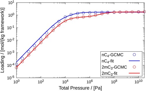
Table 4. Fitted parameters for the adsorption of pure ${\mathrm{C}}_4$ and $2\mathrm{m}{\mathrm{C}}_3$ in MFI-type zeolite at 400K.

	$k_1[1/\mathrm{Pa}]$	$q_{\max ,1}[\mathrm{mol}/(\mathrm{kgframework})]$	$k_2[1/\mathrm{Pa}]$	$q_{\max ,2}[\mathrm{mol}/(\mathrm{kgframework})]$
${\mathrm{nC}}_4$	$2.552\cdot {10}^{-4}$	0.70	$2.348\cdot {10}^{-5}$	1.02
${2\mathrm{mC}}_3$	$9.861\cdot {10}^{-5}$	0.70	$1.00\cdot {10}^{-7}$	0.90

Notes: Adsorbed loadings obtained from the GCMC simulations for the pressure range of $({10}^0-5\cdot {10}^{10})$ Pa are fitted using the dual-site Langmuir isotherm. Subscript 1 indicates site 1 (intersections between the channels) and subscript 2 indicates site 2 (channels) present inside MFI-type zeolite.

To identify the preferred sites for adsorption, snapshots of the pure components (${\mathrm{nC}}_4$ and 2m${\mathrm{C}}_3$) inside the MFI-type zeolites are shown in Figure 8. ${\mathrm{nC}}_4$ does not exhibit a strong preference for any of the adsorption sites Figure 8(a,b). 2m${\mathrm{C}}_3$ prefers the intersection between the channels in the MFI-type zeolite Figure 8(c,d). The presence of a branch (methyl group) in the hydrocarbon chain makes it energetically less favourable for 2m${\mathrm{C}}_3$ to adsorb inside the channels Figure 8(c) [42]. At higher pressures $(\ge {10}^6\mathrm{Pa})$, 2m${\mathrm{C}}_3$ starts adsorbing inside the channels Figure 8(d). At the intersections (site 1) in MFI-type zeolite, the maximum possible loadings is 4 molecules/(unit cell) or ca. 0.70 mol/(kg framework). Therefore, $q_{\max }$ is assigned this value at site 1 for both ${\mathrm{nC}}_4$ and ${2\mathrm{mC}}_3$ Table 4.Figure 9 shows the comparison between the mixture isotherm data, calculated using IAST, SIAST, SEI and GCMC. Even at higher pressures $(\sim {10}^8\mathrm{Pa})$, the adsorbed loading values estimated by SIAST and SEI are almost identical to those generated by GCMC simulations. IAST underpredicts the value of the adsorbed loading for 2m${\mathrm{C}}_3$ at higher pressure $(\ge {10}^5\mathrm{Pa})$. The reason for this deviation is again the preference of one adsorption site over the other. E.g. at an intersection (site 2), 2m${\mathrm{C}}_3$ molecules will be affected by the adsorption of only those ${\mathrm{nC}}_4$ molecules which are also adsorbed on that site. IAST again fails to capture this effect.

4.2. Breakthrough curve simulations

The influence of SEI and SIAST on the simulation of breakthrough curves has been studied. Figure 10(a) shows the breakthrough curves at the exit of the adsorber column for the ${\mathrm{CO}}_2$ – ${\mathrm{C}}_3$ mixture $(10\mathrm{\%}{\mathrm{CO}}_2,10\mathrm{\%}{\mathrm{C}}_3,80\mathrm{\%}\mathrm{helium})$ in MOR-type zeolite at 300K and ${10}^5$Pa. The weakly adsorbing component leaves the adsorber first. In the ${\mathrm{CO}}_2$-${\mathrm{C}}_3$ mixture, ${\mathrm{C}}_3$ is the weakly adsorbing component. It also exhibits a roll-up behaviour. This occurs when the molar concentration of the adsorbing species in the gas phase exceeds its inlet concentration $(c_i/c_{\mathrm{in},i}>1)$ [48]. Similarly, Figure 10(b) shows the breakthrough curves for a mixture of ${\mathrm{nC}}_4$ and ${2\mathrm{mC}}_3(10\mathrm{\%}{\mathrm{nC}}_4,10\mathrm{\%}{2\mathrm{mC}}_3,80\mathrm{\%}\mathrm{helium})$ in MFI-type zeolite at 400K and ${10}^6$Pa. In this case, ${2\mathrm{mC}}_3$ is the weakly adsorbing species. Therefore, there is an early onset of the breakthrough curve for ${2\mathrm{mC}}_3$ compared to ${\mathrm{nC}}_4$.

Figure 8. Typical snapshots of adsorption of pure C${}_4$ and 2mC${}_3$ molecules in MFI-type zeolite at 400K using GCMC simulations. (a) adsorption of ${\mathrm{C}}_4$ at ${10}^4$Pa, (b) adsorption of ${\mathrm{C}}_4$ at ${10}^8$Pa, (c) adsorption of ${2\mathrm{mC}}_3$ at ${10}^4$Pa and (d) adsorption of ${2\mathrm{mC}}_3$ at ${10}^8$Pa. Site 1 represents the intersections and site 2 represent the channels present inside the MFI-type zeolite.

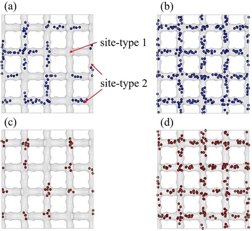
Figure 9. Adsorption isotherms of an equimolar mixture ${\mathrm{nC}}_4$ and ${2\mathrm{mC}}_3$ in MFI-type zeolite at 400K. A comparison is drawn between the adsorbed loadings calculated using GCMC, IAST, SIAST and SEI. The pressure range $({10}^2-{10}^8)$ Pa is considered for the calculations performed using IAST, SIAST and SEI. For GCMC simulations, the pressure range is $({10}^4-{10}^8)$ Pa. Cross marks represent GCMC calculations, triangles are used for IAST, circles for SIAST and squares for SEI.

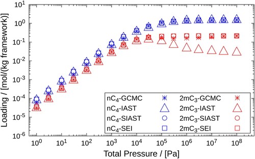
Figure 10. Comparison of breakthrough curves obtained on implementing IAST, SIAST and SEI to the breakthrough curve model. Separation of (a) ${\mathrm{CO}}_2$-${\mathrm{C}}_3$ mixture using MOR-type zeolite at 300K and ${10}^5$Pa, (b) ${\mathrm{nC}}_4$-${2\mathrm{mC}}_3$ mixture using MFI-type zeolite at 400K and ${10}^6$Pa. Each component constitutes $10\mathrm{\%}$ of the mixture in the gas phase. The remaining amount is a non adsorbing carrier gas (helium). Solid lines represent the implementation of SEI. Dashed-dotted lines are used for the SIAST model and dashed lines are used for the IAST model.

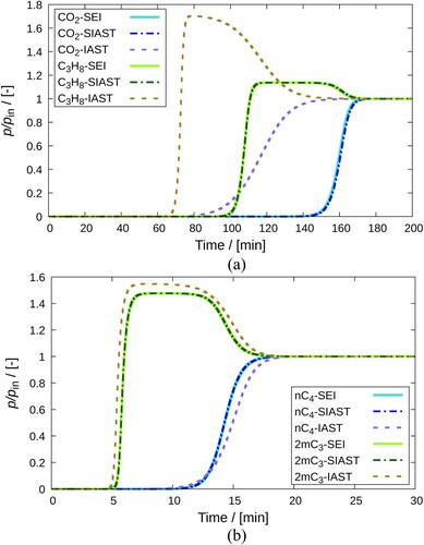
It is clearly observed from Figure 10(a,b) that the breakthrough curves calculated using IAST are quite different from those calculated using SIAST and SEI. Stronger differences can be observed in the case of ${\mathrm{CO}}_2$-${\mathrm{C}}_3$. This is due to the highly inaccurate prediction of the adsorbed mixture loadings by IAST. Implementation of SEI and SIAST yields breakthrough curves that coincide with each other for both case studies.

It is important to consider the run time of the simulations. The variation in the run time on implementing these techniques (IAST, SIAST and SEI) to the breakthrough model are shown in Table 5. The breakthrough model with SEI implementations leads to the fastest simulations. This is because of the explicit nature of the SEI model. The SIAST model is slower than the SEI model but much faster than the model with IAST implementations. The breakthrough simulations using SEI are about ca. 3 times faster than the simulations using SIAST for both case studies. Again, implementing SIAST leads to calculations ca. 20 times faster than using IAST for both case. The reason for slower IAST calculations is the use of multi-site adsorption isotherms for the pure components. IAST involves two iterative processes: (1) calculation of the spreading pressure and (2) the pure component pressure $(p_{\mathrm{pure}})$ which is the inverse of the spreading pressure. The use of single-site Langmuir isotherms yields an explicit expression for the pure pressure $(p_{\mathrm{pure}})$ by inverting the spreading pressure which is not possible for multi-site Langmuir isotherms. In the absence of an explicit expression, one has to adopt an iterative scheme, such as bisection or Newton-Raphson method, to solve for $p_{\mathrm{pure}}$. This makes the IAST calculations time consuming. In the SIAST model, we do not consider the multi-site isotherm at once. Rather, at each site, a part of the multi-site isotherm is used which is a single-site Langmuir isotherm in itself and for which there is an analytic expression for the inverse of the spreading pressure. As an explicit expression for the pure component pressure is available for each adsorption site, only the spreading pressure $(\mathrm{\Psi })$ is computed iteratively in the SIAST model. This reduces the simulation run-time significantly compared to IAST. That is why the simulation speed for SIAST and SEI differ only by a factor of ca. 3. If the spreading pressure function cannot be inverted to an explicit expression at each site, then SIAST will also involve the above mentioned two iterative processes. Consequently, SIAST will lose its advantage over IAST in terms of the speed of calculations. The simulation run time shown in Table 5 are obtained for IAST and SIAST when bisection method is used for solving the system of implicit equations.

Table 5. Variation in simulation run time $(t_{\mathrm{run}})$ for the breakthrough curve model on implementing SEI, SIAST and IAST.

	$t_{\mathrm{run}}[\mathrm{hrs}](\mathrm{case}1)$	$t_{\mathrm{run}}[\mathrm{hrs}](\mathrm{case}2)$
$\mathrm{IAST}$	17.4	2.94
$\mathrm{SIAST}$	0.92	0.15
$\mathrm{SEI}$	0.33	0.05

Notes: Comparisons are drawn for both case studies: ${\mathrm{CO}}_2-{\mathrm{C}}_3$ (case 1) and ${\mathrm{nC}}_4-{2\mathrm{mC}}_3$ mixtures (case 2). These simulations were run on a local supercomputer at Delft University of Technology (HAL9000).

5. Conclusions

A comparison between Ideal Adsorbed Solution Theory (IAST), Segregated Ideal Adsorbed Solution Theory (SIAST), and Segregated Explicit Langmuir (SEI) has been performed by calculating the adsorption isotherms and breakthrough curves for the case studies: (1) equimolar mixture of ${\mathrm{CO}}_2$-${\mathrm{C}}_3$ in MOR-type zeolite at 300K, and (2) equimolar mixture of ${\mathrm{nC}}_4$-${2\mathrm{mC}}_3$ mixture in MFI zeolite at 400K. The mixture isotherms predicted by SEI and SIAST are in excellent agreement with the GCMC simulation data. When the adsorbents have different adsorption sites and the components in the mixture prefer certain sites over the others, SIAST and SEI provide much better predictions of adsorbed loadings than IAST. We have observed this in both case studies. IAST underestimates the adsorption loadings for the less adsorbing components (${\mathrm{C}}_3$ in case 1, and ${2\mathrm{mC}}_3$ in case 2) and overpredicts the counterparts with stronger affinity for adsorption. This is due to the assumption of uniform adsorbents in the IAST model. Due to this assumption, IAST cannot capture the actual competition experienced by different components at each site. In case study 1, ${\mathrm{CO}}_2$ prefers the smaller pockets inside MOR-type zeolite whereas ${\mathrm{C}}_3$ prefers the larger pockets. At higher pressures, when both pockets are filled with ${\mathrm{CO}}_2$ and ${\mathrm{C}}_3$, the competitive adsorption in each type of pockets is different due to their preferences. Similar observations are made in the 2nd case study. IAST again underpredicts the adsorbed loadings of ${2\mathrm{mC}}_3$ in MFI-type zeolite. ${2\mathrm{mC}}_3$ preferentially adsorbs at the intersections between the channels inside MFI-type zeolite. At higher total pressure ($p_{\mathrm{tot}}>{10}^6\mathrm{Pa}$), ${2\mathrm{mC}}_3$ starts adsorbing inside the channels. In sharp contrasts, ${\mathrm{nC}}_4$ does not have a strong preference for any of the two sites in MFI-type zeolite (channels and intersections). If the adsorbents have very distinct adsorption sites and the adsorbates prefer a certain site over others, the predicted loadings by IAST will generally not be accurate. SEI and SIAST can provide better estimations compared to IAST. The major advantage of SEI is that it involves only explicit equations which makes it computationally much cheaper and improves numerical stablity. This is beneficial when equilibrium loadings need to be calculated within a breakthrough curve model both in terms of speed and accuracy. In this study, we have observed that the breakthrough curve simulations with the SEI model are ca. 3 times faster than the simulations with the SIAST model. However, the major improvement in the run time of the simulations is observed between SIAST and IAST when mulit-site isotherms are used for the pure components. Breakthrough model with SIAST implementations is found to be about 20 times faster than implementing IAST. This is because IAST involves two iterative processes: (1) calculation of the spreading pressure $(\mathrm{\Psi })$, and (2) calculation of the pure component pressure $(p_{\mathrm{pure}})$ which is the inverse of the spreading pressure function. In case of SIAST, the inverse of Ψ is generally an explicit function for each type of adsorption site. Hence, no iterations are required to calculate $p_{\mathrm{pure}}$. If the inverse of Ψ at each adsorption site does not lead to an explicit function, SIAST will lose its advantage over IAST in terms of the speed of calculations. The enhancement in the simulation run time on implementing SEI and SIAST will be very beneficial in screening a large number of adsorbents for a certain separation process, which is otherwise very time consuming on implementing IAST. This comparison is valid only for adsorbents with multiple distinct adsorption sites. For adsorbents with single type of adsorption sites, IAST and SIAST are identical by definition.

Disclosure statement

No potential conflict of interest was reported by the author(s).

Additional information

Funding

TJHV acknowledges NWO-CW for a VICI grant. This work was sponsored by NWO Domain Science for the use of supercomputer facilities. This work is part of the Advanced Research Center for Chemical Building Blocks, ARC-CBBC, which is co-funded and co-financed by the Netherlands Organization for Scientific Research (NWO) and the Netherlands Ministry of Economic Affairs and Climate Policy. S. R. G. B. was supported by [grant number POSTDOC_21_00069] funded by Consejería de Universidades, Investigación e Innovación, Junta de Andalucía.

References

- C.L. Cavalcante, Lat. Am. Appl. Res. 30, 357–364 (2000).
- P. Pullumbi, F. Brandani and S. Brandani, Curr. Opin. Chem. Eng. 24, 131–142 (2019). doi:10.1016/j.coche.2019.04.008.
- Q.U. Jiuhui, J. Environ. Sci. 20 (1), 1–13 (2008). doi:10.1016/S1001-0742(08)60001-7.
- M.A. Alghoul, M.Y. Sulaiman, B.Z. Azmi, K. Sopian and M.A. Wahab, Anti-Corros. Method. M 54, 225–229 (2007). doi:10.1108/00035590710762366.
- C.H. Yu, C.H. Huang and C.S. Tan, Aerosol. Air. Qual. Res. 12, 745–769 (2012). doi:10.4209/aaqr.2012.05.0132.
- W. John Thomas and B. Crittenden, Adsorption Technology and Design (Butterworth-Heinemann, Woburn, 1998).
- A. Poursaeidesfahani, E. Andres-Garcia, M. de Lange, A. Torres-Knoop, M. Rigutto, N. Nair, F. Kapteijn, J. Gascon, D. Dubbeldam and T.J.H. Vlugt, Microporous. Mesoporous. Mater. 277, 237–244 (2019). doi:10.1016/j.micromeso.2018.10.037.
- D. Frenkel and B. Smit, Understanding Molecular Simulation: From Algorithms to Applications (Academic Press, San Diego, 2002).
- E.C. Markham and A.F. Benton, J. Am. Chem. Soc. 53, 497–507 (1931). doi:10.1021/ja01353a013.
- A.L. Myers and J.M. Prausnitz, AICHE J 11, 121–127 (1965). doi:10.1002/(ISSN)1547-5905.
- K.S. Walton and D.S. Sholl, AICHE J 61, 2757–2762 (2015). doi:10.1002/aic.14878.
- O. Talu and I. Zwiebel, AICHE J 32, 1263–1276 (1986). doi:10.1002/(ISSN)1547-5905.
- A. Erto, A. Lancia and D. Musmarra, Microporous. Mesoporous. Mater. 154, 45–50 (2012). doi:10.1016/j.micromeso.2011.10.041.
- R. Krishna and J.M. van Baten, ACS Omega 6, 15499–15513 (2021). doi:10.1021/acsomega.1c02136.
- H. Renon and J.M. Prausnitz, AICHE J 14, 135–144 (1968). doi:10.1002/(ISSN)1547-5905.
- G.M. Wilson, J. Am. Chem. Soc. 86, 127–130 (1964). doi:10.1021/ja01056a002.
- A. Fredenslund, R.L. Jones and J.M. Prausnitz, AICHE J 21, 1086–1099 (1975). doi:10.1002/(ISSN)1547-5905.
- Y.G. Chung, P. Bai, M. Haranczyk, K.T. Leperi, P. Li, H. Zhang, T.C. Wang, T. Duerinck, F. You and J.T. Hupp, Chem. Mater. 29, 6315–6328 (2017). doi:10.1021/acs.chemmater.7b01565.
- R. Krishna, Sep. Purif. Technol. 194, 281–300 (2018). doi:10.1016/j.seppur.2017.11.056.
- D.D. Do, Adsorption Analysis: Equilibria and Kinetics (with CD Containing Computer MATLAB Programs), Series On Chemical Engineering (World Scientific Publishing, London, 1998).
- R.A. Koble and T.E. Corrigan, Ind. Eng. Chem. 44, 383–387 (1952). doi:10.1021/ie50506a049.
- J.A. Swisher, L.C. Lin, J. Kim and B. Smit, AICHE J 59, 3054–3064 (2013). doi:10.1002/aic.14058.
- R. Krishna and J.M. van Baten, Sep. Purif. Technol. 61, 414–423 (2008). doi:10.1016/j.seppur.2007.12.003.
- R. Krishna and J.M. van Baten, Chem. Phys. Lett. 446, 344–349 (2007). doi:10.1016/j.cplett.2007.08.060.
- S. Sircar, Ind. Eng. Chem. Res. 30, 1032–1039 (1991). doi:10.1021/ie00053a027.
- D.P. Valenzuela, A.L. Myers, O. Talu and I. Zwiebel, AICHE J 34, 397–402 (1988). doi:10.1002/(ISSN)1547-5905.
- K. Wang, S. Qiao and X. Hu, Sep. Purif. Technol. 20, 243–249 (2000). doi:10.1016/S1383-5866(00)00087-3.
- H. Moon and C. Tien, Chem. Eng. Sci. 43, 2967–2980 (1988). doi:10.1016/0009-2509(88)80050-2.
- J.A. Ritter, S.J. Bhadra and A.D. Ebner, Langmuir 27, 4700–4712 (2011). doi:10.1021/la104965w.
- A. Tarafder and M. Mazzotti, Chem. Eng. Technol. 35, 102–108 (2012). doi:10.1002/ceat.201100274.
- U. Agarwal, M.S. Rigutto, E. Zuidema, A. Jansen, A. Poursaeidesfahani, S. Sharma, D. Dubbeldam and T.J.H. Vlugt, J. Catal. 415, 37–50 (2022). doi:10.1016/j.jcat.2022.09.026.
- D.M. Ruthven, Principles of Adsorption and Adsorption Processes (John Wiley & Sons, New York, 1984).
- T.R.C. Van Assche, G.V. Baron and J.F.M. Denayer, Ind. Eng. Chem. Res. 60, 12092–12099 (2021). doi:10.1021/acs.iecr.1c01657.
- T.R.C. Van Assche, G.V. Baron and J.F.M. Denayer, Adsorption 24, 517–530 (2018). doi:10.1007/s10450-018-9962-1.
- R. Krishna and J.M. van Baten, Sep. Purif. Technol. 76, 325–330 (2011). doi:10.1016/j.seppur.2010.10.023.
- Z. Du, G. Manos, T.J.H. Vlugt and B. Smit, AICHE J 44, 1756–1764 (1998). doi:10.1002/(ISSN)1547-5905.
- R. Krishna, B. Smit and S. Calero, Chem. Soc. Rev. 31, 185–194 (2002). doi:10.1039/b101267n.
- E. García-Pérez, I. Torrens, S. Lago, D. Dubbeldam, T.J.H. Vlugt, T.L. Maesen, B. Smit, R. Krishna and S. Calero, Appl. Surf. Sci. 252, 716–722 (2005). doi:10.1016/j.apsusc.2005.02.103.
- Dynamic sorption methods (2022). https://www.dynamicsorption.com/dynamic-sorption-method/ .
- S. Sircar, Adsorption 23, 121–130 (2017). doi:10.1007/s10450-016-9839-0.
- C. Simon, B. Smit and M. Haranczyk, Comput. Phys. Commun. 200, 364–380 (2016). doi:10.1016/j.cpc.2015.11.016.
- T.J.H. Vlugt, W. Zhu, F. Kapteijn, J. Moulijn, B. Smit and R. Krishna, J. Am. Chem. Soc. 120, 5599–5600 (1998). doi:10.1021/ja974336t.
- T.J.H. Vlugt, R. Krishna and B. Smit, J. Phys. Chem. B 103, 1102–1118 (1999). doi:10.1021/jp982736c.
- R. Krishna, B. Smit and T.J.H. Vlugt, J. Phys. Chem. A 102, 7727–7730 (1998). doi:10.1021/jp982438f.
- R.L. Burden and J.D. Faires, Numerical Analysis, Mathematics Series (PWS-Kent Publishing Company, Boston, 1993).
- W. Kast, Adsorption Aus Der Gasphase. Ingenieurwissenschaftliche Grundlagen und Technische Verfahren (Verlag Chemie, Weinheim, Germany, 1988).
- R.T. Yang, Adsorbents: Fundamentals and Applications (John Wiley & Sons, New Jersey, 2003).
- R. Krishna and R. Baur, Sep. Purif. Technol. 33, 213–254 (2003). doi:10.1016/S1383-5866(03)00008-X.
- E. Glueckauf, Trans. Faraday Soc. 51, 1540–1551 (1955). doi:10.1039/TF9555101540.
- A. Özdural, in Comprehensive Biotechnology, edited by M. Moo-Young, 2nd ed. (Academic Press, Burlington, 2011), pp. 681–695.
- D. Dubbeldam, S. Calero, D.E. Ellis and R.Q. Snurr, Mol. Simul. 42, 81–101 (2016). doi:10.1080/08927022.2015.1010082.
- D. Dubbeldam, A. Torres-Knoop and K.S. Walton, Mol. Simul. 39, 1253–1292 (2013). doi:10.1080/08927022.2013.819102.
- P.P. Ewald, Ann. Phys. 369, 253–287 (1921). doi:10.1002/(ISSN)1521-3889.
- A. Garcia-Sanchez, C.O. Ania, J.B. Parra, D. Dubbeldam, T.J.H. Vlugt, R. Krishna and S. Calero, J. Phys. Chem. C 113, 8814–8820 (2009). doi:10.1021/jp810871f.
- D. Dubbeldam, S. Calero, T.J.H. Vlugt, R. Krishna, T.L.M. Maesen and B. Smit, J. Phys. Chem. C108, 12301–12313 (2004). doi:10.1021/jp0376727.
- P. Bai, M. Tsapatsis and J.I. Siepmann, J. Phys. Chem. C 117, 24375–24387 (2013). doi:10.1021/jp4074224.
- M.G. Martin and J.I. Siepmann, J. Phys. Chem. C 102, 2569–2577 (1998). doi:10.1021/jp972543+.
- D. Dubbeldam, S. Calero and T.J.H. Vlugt, Mol. Simul. 44, 653–676 (2018). doi:10.1080/08927022.2018.1426855.
- W.E. Schiesser, The Numerical Method of Lines: Integration of Partial Differential Equations (Academic Press, San Diego, 2012).
- J.D. Anderson and J. Wendt, Computational Fluid Dynamics, Volume 206 (McGraw-Hill, New York, 1995).
- H.P. Langtangen and S. Linge, Finite Difference Computing with PDEs: A Modern Software Approach (Springer Nature, Cham, 2017).
- C.W. Shu and S. Osher, J. Comput. Phys. 77, 439–471 (1988). doi:10.1016/0021-9991(88)90177-5.
- D.I. Ketcheson, SIAM. J. Sci. Comput. 30, 2113–2136 (2008). doi:10.1137/07070485X.
- H.O.R. Landa, Development of an efficient method for simulating fixed-bed adsorption dynamics using ideal adsorbed solution theory, Ph.D. diss., Otto von Guericke Universität Magdeburg, 2016.