
 ?Mathematical formulae have been encoded as MathML and are displayed in this HTML version using MathJax in order to improve their display. Uncheck the box to turn MathJax off. This feature requires Javascript. Click on a formula to zoom.
Abstract
Two powerful theories for state-to-state chemical reactions are brought together for the first time. The first theory incorporates Regge pole positions and residues into the partial wave (PW) scattering (S) matrix. The second theory is a ‘weak’ version of Heisenberg’s Scattering Matrix Programme (wHSMP). It uses four general physical principles to suggest simple parameterised forms for the S matrix. The wHSMP is particularly useful for understanding generic structures in differential cross sections (DCSs). Our initial S matrix parameterisation has no Regge poles, but it exhibits a rainbow in the DCS using a Legendre PW series. We then introduce Regge poles for three examples into the S matrix and investigate their influence on the rainbow scattering. We find that inclusion of Regge poles ‘pushes’ the rainbow angle to larger values. We also employ Nearside-Farside (NF) PW and Local Angular Momentum PW theories, including up to three resummations. The recently introduced ‘CoroGlo’ test is used to distinguish between glory and corona scattering in the forward direction. We apply full and NF asymptotic (semiclassical) rainbow theories: the uniform and transitional Airy approximations for the farside scattering. We prove that structure in the no-pole and with-pole DCSs are examples of primary and supernumerary rainbows.
GRAPHICAL ABSTRACT
1. Introduction
A key quantity in the theory of state-to-state chemical reactions is the scattering matrix (S matrix) or scattering operator (S operator) because, in principle, they allow a complete characterisation of a reaction. For example, the S matrix permits collisional observables to be calculated, such as differential cross sections (DCSs), which contain detailed information on the mechanism and dynamics of a reaction. The interpretation of DCSs, which often exhibit complicated interference patterns, is therefore an important problem [Citation1–6].
The computation of DCSs from first principles for known initial states to known final states usually follows the following scheme:
(R1)
(R1) The reaction scheme R1 has been called ‘The Royal Road of Reaction Dynamics’ [Citation7] because of its ubiquity and importance. Despite impressive advances [Citation1–6], The Royal Road suffers from some well-known limitations, which continue to slow its progress: (a) It is difficult to calculate potential energy surfaces of sufficient accuracy for reliable use in dynamical scattering calculations. (b) Computed S matrix elements can be contaminated by numerical errors. (c) In the semiclassical (or asymptotic, ħ → 0) limit, the S matrix elements obtained in a large-scale computation often consist of long list of complex numbers, which, in more complicated cases, can be difficult (or impossible) to understand and interpret. (d) A new scattering calculation is required for a new potential energy surface and a new reaction. For additional discussion, see ref. [Citation7]. Clearly, it is desirable to investigate alternative and complementary approaches for the computation of dynamical phenomena, in particular for the calculation of DCSs.
We have recently begun exploring a simple, yet powerful, alternative approach based on a ‘weak’ version of Heisenberg’s Scattering Matrix Programme (wHSMP) [Citation7–11]. Our approach can be summarised as follows
(R2)
(R2) The reaction scheme R2 does not employ a potential energy surface – see ref. [Citation7] for a full discussion of this point. Rather it is based on Heisenberg’s fundamental insight that the S matrix contains, in principle, all the information needed to calculate dynamical phenomena [Citation12–15]. Heisenberg hoped to use general physical principles, such as unitarity, causality and analyticity to determine the S matrix. This has not yet proved possible, so in our approach, we use instead four general physical principles relevant to state-to-state chemical reactions to suggest simple, yet realistic, parametrised forms for the S matrix. We denote our five previous papers in refs. [Citation7,Citation8,Citation9,Citation10,Citation11] by H1, H2, H3, H4, H5 respectively. We have earlier explored the following topics:
In H1, we described HSMP and introduced wHSMP, applying it to the forward glory scattering of the H + D2 → HD + D reaction. Historical remarks on HSMP can also be found in H1.
In H2, we obtained a surprising result: piecewise S matrix elements using simple linear, quadratic, step-function and top-hat parameterisations can reproduce the small-angle scattering of the H + D2 → HD + D reaction.
In H3, we studied a DCS for the F + H2 → FH + H reaction using the techniques in H1 and H2. We also applied a variant of wHSMP in which the parameterised S matrix is modified using simple Gaussian-type functions suggested by results from scheme R1. We called this variant, ‘hybrid’, and denoted it, hHSMP ≡ hwHSMP.
In H4, we proved the existence of pronounced Airy rainbows, supernumerary rainbows and interference effects in product DCSs arising from attractive (or farside) scattering. We kept the modulus of the S matrix fixed and systematically varied its phase.
H5 is similar to H4, except that we kept the phase of the S matrix fixed and systematically varied its modulus. Thus, H4 and H5 together reported a systematic investigation of pronounced rainbows for a class of reactive systems.
It is also important to note that H1, H2, H3 are fundamentally different from H4, H5. In H1, H2, H3, a quadratic polynomial phase in was used for the parameterised S matrix, whereas in H4, H5, a cubic polynomial phase was employed. Here
is the total angular momentum quantum number.
It is evident from the above, that wHSMP is a practical and powerful tool, which can complement calculations from the ‘The Royal Road of Reaction Dynamics’ [Citation7–11]. In particular, the wHSMP can be used to quickly calculate DCSs from partial wave series (PWS). Then by making changes to the S matrix, we can rapidly investigate generic structures in DCSs for state-to-state chemical reactions, such as rainbows, glories and interference (Fraunhofer) effects. This is done by exploring different parameterisations for the modulus and phase of the S matrix [Citation7–11]. A useful aim is to find simple parameterisations, which are capable of describing key features of the reaction dynamics. In addition, we can also determine the values of the parameters by fitting experimental DCSs, or the results of computer simulations. Finally, we note that the parameterised S matrix elements can be refined by adding information obtained from potential energy surface(s) computations, until eventually we arrive at the S matrix from The Royal Road.
In recent years, another powerful theory has been applied to chemical reactions: it exploits the properties of the S matrix in the complex angular momentum (CAM) plane (for reviews to molecular problems, see refs. [Citation3,Citation16–21]), which is also known as Regge theory [Citation22,Citation23]. This CAM theory involves concepts such as Regge pole positions and residues, life angles, Regge and residue trajectories, surface waves etc. Interestingly, it is also well known that there is a close connection between attractive (Airy) rainbows and Regge poles, see, e.g. refs. [Citation18,Citation21,Citation24–29].
The purpose of this paper is to incorporate, for the first time, Regge poles into wHSMP. In particular, we examine how Regge poles affect rainbow scattering. More generally, our aim is to gain a better understanding of the rôle Regge pole positions and residues play in understanding interference structures in reactive DCSs.
The theory presented in this paper is for the following generic state-to-state chemical reaction:
(R3)
(R3) where vi, ji, mi and vf, jf, mf are vibrational, rotational and helicity quantum numbers for the initial and final states, respectively. It is assumed that the reaction occurs at a fixed total energy, or equivalently a fixed initial translational wavenumber. Then the PWS for the scattering amplitude can be expanded in a basis set of Legendre polynomials. There are also many approximate theories for chemical reactions that use a Legendre PWS. Thus, the theory and results in this paper should have a wide utility.
This paper is organised as follows. Section 2 presents the general physical principles used in wHSMP for the design of the S matrix. Sections 3 and 4 describe the parameterised forms that we employ in our PWS computations for the pre-exponential and phase components of the S matrix respectively. The theoretical techniques we use are presented in Section 5, which all use a PWS. We summarise in Section 6 the asymptotic (semiclassical ≡ SC) techniques we use to prove the existence of rainbows; in particular, we use uniform and transitional Airy SC approximations. In Section 7, we numerically sum the Legendre PWS for the scattering amplitude to calculate DCSs and Local Angular Momenta (LAMs) for the reference case of a smooth-step parameterisation for the S matrix. This example does not contain any explicit Regge poles in the PWS. In Section 8, we investigate the influence of Regge poles of the form in the PWS. Here
is the partial residue and
is the position of the nth Regge pole. In Section 9, we present and discuss our DCS results when Regge poles are included for three examples. An interesting finding is that a Regge pole(s) ‘pushes’ the rainbow angle to larger angles in the DCS compared to the non-pole DCS. In both Sections 7 and 9, we apply the recently introduced ‘CoroGlo’ test [Citation30,Citation31], which lets us distinguish in a simple way between corona and glory scattering in a reactive DCS at small angles. We also apply Nearside-Farside (NF) theory [Citation27,Citation32,Citation33] and LAM theory [Citation34,Citation35] together with resummations of the PWS [Citation34–40]. Conclusions are in Section 10. The Appendix discusses a many-pole example in more detail.
2. Weak version of Heisenberg’s S matrix programme
In this section, we describe the assumptions of wHSMP [Citation7]. It is based on four general physical principles relevant to chemical reactions. Our design strategy for the construction of the S matrix elements is based on them. Note that no potential energy surface is used. As usual [Citation7–11], we employ a modified S matrix element, denoted . The four assumptions of wHSMP are:
The forces responsible for chemical reactions are short ranged, of the order of 10−10 m. This implies
as
Conservation of probability holds. This implies the S matrix is unitary with
Under semiclassical (SC) or asymptotic (ħ → 0) conditions, namely,
In the classical limit, we require a head-on collision to correspond to backward (or rebound) scattering of the products.
In Assumption 3, by ‘analytic’ we include functions with poles and branch points, as is usual in S matrix theory [Citation7].
Assumption 3 was used in a weaker form in H2 and H3, where
In Assumption 4 and elsewhere, we use the reactive scattering angle,
Using the above physical assumptions for wHSMP, we follow H1–H5 and parametrise for real
in the form
(1)
(1) where the subscript ‘X’ = ‘step’, ‘pole’, or ‘s/p ≡ step/pole’, is an optional label added sometimes for clarity, and which are defined below,
is a real normalisation constant, and
is a real phase. For the pre-exponential factor,
, there are two possibilities:
When there are no explicit Regge poles,
When there are explicit Regge poles present of the type,
In both cases, we must choose and
so that
for all
.
3. Parameterisation of
For the two possibilities mentioned in Section 2, we construct ‘smooth step’ and ‘pole sum’ parameterisations for , as follows:
3.1. Smooth step
We use a simple smooth-step parameterisation, previously employed in H1 and H4, modelled on the H + D2 reaction, namely
(2)
(2) where
is the ‘cut off’ value of
and
acts as a ‘diffuseness’ parameter in
space. Both
and
are positive, although not necessarily integers.
In passing, we note that in the CAM plane, , has an infinite number poles lying on a line in the first and fourth quadrants of the complex
plane [Citation7,Citation41]. However this property is not required, since we only use,
, for
= 0, 1, 2, … and its continuation to real values of
. The continuation is automatically supplied by Equation (Equation2
(R2)
(R2) ). We also sometimes write Equation (Equation1
(R1)
(R1) ) more explicitly as
(3)
(3) Figure shows graphically, for the standard values of the parameters in Section 7, the properties that we derive analytically in this section, and the next one, for the smooth-step parameterisation.
Figure 1. S matrix data for the smooth-step parameterisation. The values of the parameters are given in section 7. (a) versus
. (b)
versus
. The maximum and local minimum of the
curve define the glory angular momentum variables,
and
, respectively, which are indicated by orange dashed lines and arrows. The rainbow angular momentum variable,
, is indicated by a pink dashed line and arrow. (c)
versus
. The red dashed line and arrow indicate
and
for the N scattering. The blue dashed line and arrows indicate
as well as
and
for the F scattering. Also shown is
, which is located at the minimum of the
curve, where
(pink arrow and dashed lines) together with
and
, which satisfy
. The three branches of the deflection function are labelled 1 (N, red) and 2, 3 (F, both blue). (d)
versus
. Also marked are,
,
,
, with dashed lines and arrows, and the N and F angular zones. [See colour online].
![Figure 1. S matrix data for the smooth-step parameterisation. The values of the parameters are given in section 7. (a) |S~step(J)| versus J. (b) argS~step(J)/rad versus J. The maximum and local minimum of the argS~step(J)/rad curve define the glory angular momentum variables, Jg1 and Jg2, respectively, which are indicated by orange dashed lines and arrows. The rainbow angular momentum variable, Jr, is indicated by a pink dashed line and arrow. (c) Θ~step(J)/deg versus J. The red dashed line and arrow indicate +θR and J1=J1(θR) for the N scattering. The blue dashed line and arrows indicate −θR as well as J2=J2(θR) and J3=J3(θR) for the F scattering. Also shown is Jr, which is located at the minimum of the Θ~step(J)/deg curve, where Θ~step(J=Jr)=−θRr(pink arrow and dashed lines) together with Jg1 and Jg2, which satisfy Θ~step(Jg1orJg2)=0. The three branches of the deflection function are labelled 1 (N, red) and 2, 3 (F, both blue). (d) (2J+1)|S~step(J)| versus J. Also marked are, Jg1, Jr, Jg2, with dashed lines and arrows, and the N and F angular zones. [See colour online].](/cms/asset/b47677e7-a515-4fe3-8436-38c43e6c05a0/tmph_a_2198616_f0001_oc.jpg)
3.2. Pole sum
We first define a ‘pole sum’ [Citation21,Citation42,Citation43] by
(4)
(4) where
is a positive integer, and
and
are complex numbers. When
is allowed to take complex values in the CAM plane,
and
correspond to the position and partial residue of the nth Regge pole respectively. For this case, we sometimes label Equation (Equation1
(R1)
(R1) ) in the form
(5)
(5)
The form in Equation (Equation4(1)
(1) ) is suggested by the Mittag-Leffler theorem for the expansion of a meromorphic function in terms of its poles.
In passing, we note that the full residue of at the pole,
, is, by definition,
although we do not need this result in the present paper.
3.3. Smooth-step + pole parameterisation
We also define the sum of the smooth-step and pole parameterisations, denoted, . We have
(6)
(6) In Equation (Equation6
(3)
(3) ),
is a damping factor needed to ensure convergence of the PWS when
is present. We use
(7)
(7) where
and
are positive parameters. Note that
is not needed when
is absent. Finally, we sometimes write
(8)
(8) Since
in Equation (Equation8
(5)
(5) ) is complex-valued [because of the pole sum in Equation (Equation6
(3)
(3) )], we have
, although it is true that
.
4. Parameterisation of
The equations presented below are for the smooth-step parameterisation, for which . When Regge poles are present, we have,
. Then the equations needed are modifications of the smooth-step case – this is discussed in Section 9.
It was shown in H4 and H5, that to describe rainbow scattering, has to be a cubic (or higher) polynomial in
. We write
(9)
(9) where
are the four real phase parameters with
, and not to be confused with the partial residue,
, in Equation (Equation4
(1)
(1) ).
An important quantity in the asymptotic (ħ → 0) or SC theory of rainbows is the derivative of , which is called the quantum defection function (QDF) and written
[Citation44]. For the smooth-step parameterisation, we have from Equation (Equation9
(6)
(6) )
(10)
(10) Next, we must choose the phase parameters in
. We proceed as follows:
The PWS DCSs and SC DCSs are independent of the value of
Equation (Equation10
The parameters
The relation between and
has been worked out in H4 using the properties,
and
. Here the prime indicates differentiation. The results for the smooth-step parameterisation are
(11)
(11) and
(12)
(12) Equations (Equation11
(8)
(8) ) and (Equation12
(9)
(9) ) let us define in a convenient way the coefficients of the cubic phase in terms of
and
, (also knowing,
and
). Since
,
and
are always positive in our applications, we see that
is always negative, whereas
is always positive.
To summarise, in the representation, we have for the cubic phase
(13)
(13) together with
(14)
(14)
Another useful representation [Citation10], makes an exact Taylor expansion of in Equation (Equation13
(10)
(10) ) about the point
. We find
(15)
(15) together with
(16)
(16) and
(17)
(17) Equations (Equation16
(13)
(13) ) and (Equation17
(14)
(14) ) let us confirm that
and
, respectively.
From Equation (Equation16(13)
(13) ), we can obtain explicit formulae for the stationary points
,
,
used in the SC theory, see Figure (c). Solving,
, for the N scattering gives
(18)
(18) whilst solving,
, for the F scattering results in
(19)
(19) and
(20)
(20)
5. Partial wave theory
Here we summarise the partial wave theory that we require and establish our notations. In particular, we outline the ‘CoroGlo’ test, nearside-farside (NF) and local angular momentum (LAM) theory, and resummations of the PWS.
5.1. Partial wave series
Since mi = mf = 0 in reaction R3, the PWS for the scattering amplitude can be expanded, as usual, in a basis set of Legendre polynomials
(21)
(21) where
is a Legendre polynomial of degree
,
is the reactive scattering angle and
is the incident translational wavenumber. In practice, the upper limit of infinity in the PWS is replaced by a finite value,
, assuming that all partial waves with
are negligible. The DCS is then given by
(22)
(22)
In our applications, the PWS of Equation (Equation21(18)
(18) ) contains about 100 numerically significant terms making its physical interpretation difficult or impossible. We also have the estimate,
, where
is the reaction radius.
Our angular distributions in Sections 7 and 9 show that the full DCSs computed from Equations (Equation21(18)
(18) ) and (Equation22
(19)
(19) ) exhibit a forward peak accompanied by oscillatory structures. To help understand these structures, we first analyse the small-angle scattering using the newly introduced ‘CoroGlo’ test [Citation30,Citation31]. For the scattering at larger angles, we make a NF decomposition of the scattering amplitude. These topics are outlined in the next two sections.
5.2. CoroGlo test
The recently introduced ‘CoroGlo’ test [Citation30,Citation31] lets us distinguish at small-angles in a DCS, whether the peak at arises from a corona or from a glory. Now both a corona and a glory give rise to a peak in the DCS(
) at
, accompanied by oscillations at larger angles displaying maxima. A corona in molecular collisions is usually modelled by Fraunhofer scattering from a hard-sphere [Citation30], whereas a glory arises from N, F interference, as illustrated in Figures and . The CoroGlo test lets us distinguish, in the asymptotic limit, between these two possibilities from the ratio of the DCS(
) at
to the value of the DCS at its adjacent maximum. We have: [Citation30]
corona diffraction ratio (CDR) ≈ 57.1
glory diffraction ratio (GDR) ≈ 6.2
Figure 2. Plots of PWS dDCSs and PWS LAMs versus , for the smooth-step parameterisation. The values of the parameters are given in section 7. (a) Logarithmic plots of the full and N,F dDCSs for the angular range,
, for resummation parameters of
,1,2,3, together with the rainbow angle,
. (b) Logarithmic plots of the full and N,F dDCSs for the angular range,
, for
. (c) Plots of the full and N,F LAMs for the angular range,
, with r = 1. The light blue curve indicates the angular range where the F LAM is non-physical. (d) Plots of the full and N,F LAMs for the angular range,
, with
. The pink arrows at
and
in (b) and (d) indicate the positions of the maxima for the primary rainbow and first supernumerary rainbow, respectively, for the uAiry asymptotic (SC) approximation of Section 6.3. [See colour online].
![Figure 2. Plots of PWS dDCSs and PWS LAMs versus θR, for the smooth-step parameterisation. The values of the parameters are given in section 7. (a) Logarithmic plots of the full and N,F dDCSs for the angular range, θR=0∘−180∘, for resummation parameters of r=0,1,2,3, together with the rainbow angle, θRr=40.0∘. (b) Logarithmic plots of the full and N,F dDCSs for the angular range, θR=0∘−60∘, for r=1. (c) Plots of the full and N,F LAMs for the angular range, θR=0∘−180∘, with r = 1. The light blue curve indicates the angular range where the F LAM is non-physical. (d) Plots of the full and N,F LAMs for the angular range, θR=0∘−60∘, with r=1. The pink arrows at θR≈35.6∘ and θR≈20.8∘ in (b) and (d) indicate the positions of the maxima for the primary rainbow and first supernumerary rainbow, respectively, for the uAiry asymptotic (SC) approximation of Section 6.3. [See colour online].](/cms/asset/cee51f52-c840-4a85-9884-bae52b89700e/tmph_a_2198616_f0002_oc.jpg)
Figure 3. Comparison of PWS and SC results for dDCSs and LAMs, all plotted versus , for the smooth-step parameterisation. The values of the parameters are given in Section 7. (a) Full PWS dDCS and full, N,F SC dDCSs for the angular range,
. (b) Full PWS and full, N,F SC dDCSs for the angular range,
. (c) Full PWS LAM and full, N,F SC LAMs for the angular range,
. (d) Full PWS LAM and full, N,F SC LAMs for the angular range,
. The pink arrows at
and
in (b) and (d) indicate the positions of the maxima for the primary rainbow and first supernumerary rainbow, respectively, for the uAiry asymptotic (SC) approximation of Section 6.3. The pink arrows mark the rainbow angle,
. [See colour online].
![Figure 3. Comparison of PWS and SC results for dDCSs and LAMs, all plotted versus θR, for the smooth-step parameterisation. The values of the parameters are given in Section 7. (a) Full PWS dDCS and full, N,F SC dDCSs for the angular range, θR=0∘−180∘. (b) Full PWS and full, N,F SC dDCSs for the angular range, θR=0∘−60∘. (c) Full PWS LAM and full, N,F SC LAMs for the angular range, θR=0∘−180∘. (d) Full PWS LAM and full, N,F SC LAMs for the angular range, θR=0∘−60∘. The pink arrows at θR≈35.6∘ and θR≈20.8∘ in (b) and (d) indicate the positions of the maxima for the primary rainbow and first supernumerary rainbow, respectively, for the uAiry asymptotic (SC) approximation of Section 6.3. The pink arrows mark the rainbow angle, θRr=40.0∘. [See colour online].](/cms/asset/b7a4e1f0-e16e-4a84-8837-998e2ad9df87/tmph_a_2198616_f0003_oc.jpg)
The values of 57.1 and 6.2, above, are the diffraction ratios for a corona and glory respectively. When applied to DCSs for chemical reactions, different values can occur and may indicate the presence of other mechanisms in the angular scattering. For example, in reference [Citation30] a ratio of 2.6 was found for a state-to-state transition in the H + HD → H2 + D reaction, which was shown to arise from the additional presence of rainbow scattering at small angles.
The CoroGlo test does not prove the presence of e.g. glory scattering. To do this, we must construct the asymptotic (SC) limit of the PWS (21). See Section 6.
The CoroGlo test does not usually apply to elastic or inelastic DCSs, because there is often a contribution to the small-angle scattering from the long-range attractive interaction potential, which is usually absent in the reactive case.
5.3. Nearside-farside decomposition
We exactly decompose the full scattering amplitude into the sum of two contributing terms, the N and F subamplitudes [Citation27,Citation32,Citation33].
(23)
(23) where
(24)
(24) with
(25)
(25) and
is a Legendre function of the second kind. Similar to Equation (Equation22
(19)
(19) ), the corresponding N and F DCSs are defined by
(26)
(26)
Using the asymptotic properties of the and
in the limit
, we obtain, e.g. refs. [Citation27,Citation33].
which have a standard travelling N,F angular waveinterpretation.
5.4. Local angular momentum nearside-farside decomposition
A local angular momentum (LAM) analysis can also be used to provide information on the total angular momentum variable that contributes to the scattering at an angle , under semiclassical conditions [Citation34,Citation35]. It is defined by
(27)
(27) The same idea can also be applied to the N and F subamplitudes in Equation (Equation23
(20)
(20) ). The corresponding N, F LAMs are defined by [Citation34,Citation35]
(28)
(28)
Note that the args in Equations (Equation27(24)
(24) ) and (Equation28
(25)
(25) ) are not necessarily principal values in order that the derivatives be well defined.
In Equations (Equation24(21)
(21) )–(Equation26
(23)
(23) ) and (28), we have used the Fuller NF decomposition [Citation45]. Note that NF DCS and NF LAM theories have been reviewed by Child [Citation3, section 11.2].
5.5. Resummation of the partial wave series
It is known that a resummation [Citation34–40] of the PWS (21) can markedly improve the physical effectiveness of the N,F decomposition (23). Although we have investigated resummation orders of , 1, 2, and 3 in this paper, we present below the working equations for
and for
[no resummation, i.e. Equation (Equation21
(18)
(18) )]. This is because resummation cleans the N,F DCSs of unphysical oscillations, and we find the biggest effect occurs on going from
to
. Further resummations,
to
and
to
have a smaller cleaning effect. A detailed account of resummation has been given by Totenhofer et al. [Citation40] for a Legendre PWS.
Firstly, we write Equation (Equation21(18)
(18) ) in the more compact form
(29)
(29) where
, and the superscript zeroindicates that
. i.e.
. Then for
, the resummed scattering amplitude is [Citation34–40]
(30)
(30) where
(31)
(31) with
. In addition, Equation (Equation30
(27)
(27) ) assumes that
. We determine the complex-valued resummation parameter
, in Equations (Equation30
(27)
(27) ) and (Equation31
(28)
(28) ) by solving
, which yields
.
The NF decomposition for the resummation case is then
(32)
(32) where the N,F
resummed subamplitudes are
(33)
(33)
An alternative form, equivalent to Equation (Equation33(30)
(30) ) is [Citation34,Citation40]
with
.
The corresponding N,F resummed DCSs are then
(34)
(34) Note that the full DCSs for
and
are numerically identical at a given value of
.
N,F LAMs for can also be defined using Equation (Equation28
(25)
(25) ). We have
(35)
(35) Again the full LAMs for
and
are numerically identical at a given value of
.
6. Asymptotic (semiclassical) representations for
6.1. Introduction
The asymptotic (semiclassical ≡ SC) theory of rainbow scattering for reactive systems possessing deflection functions similar to Figure (c) is well established [Citation3,Citation16]. So in this section, we just present the working formulae for the asymptotic N and F subamplitudes, denoted, and
respectively. Note that we use superscript
to label the N and F subamplitudes, respectively, to avoid confusion with the PWS subamplitudes,
and
, which are defined by Equations (Equation24
(21)
(21) ) and (Equation33
(30)
(30) ) respectively. The full SC scattering amplitude is therefore
(36)
(36)
The corresponding full SC DCS is
(37)
(37) and the N and F SC DCSs are given by
The SC theory uses the continuation of , with
= 0, 1, 2, … , to real values of
, which we denote, as usual, by
, i.e. the S matrix elements are now considered to be a continuous function of the total angular momentum variable. An important role in the asymptotic analysis is played by the quantum deflection function,
, for the smooth-step parameterisation from Equations (Equation9
(6)
(6) ) and (Equation10
(7)
(7) ):
(38)
(38) As previously, the arg in Equation (Equation38
(35)
(35) ) is not necessarily the principal value in order that the derivative be well defined.
Figure (c) shows a graph of versus
for the standard values of the S matrix parameters used in Section 7 for rainbow scattering for the smooth-step parameterisation. We note the following properties in Figure (c), which are used below in the SC analysis:
The rainbow angular momentum variable,
For
For
For
The real roots are ordered,
For
Two glory angular momenta,
There is a 4th branch in the
The angular momenta
In the following, we adopt the following notations
(39)
(39) and
(40)
(40) where
and similarly for the second derivative,
.
6.2. Definitions
Before describing the uniform and transitional SC approximations, we first define the following phases and ‘classical-like’ DCSs, as they are needed in the expressions below. There are four SC N and F phases associated with ,
,
and
, which are given by [Citation10,Citation28]
(41)
(41)
(42)
(42)
(43)
(43)
(44)
(44)
There are also three ‘classical-like’ N and F DCSs defined by [Citation10,Citation28]
(45)
(45)
(46)
(46)
(47)
(47) Since,
, there is no analogous expression to Equations (Equation45
(42)
(42) )–(Equation47
(44)
(44) ) for the case,
.
6.3. Asymptotic (SC) rainbow analysis of the farside scattering
For the farside scattering, the stationary phase condition is
(48)
(48) In Figure (c), there are two real roots of Equation (Equation48
(45)
(45) ) for a given value of
, provided
, which is the bright side of the rainbow. At
, the two real roots coalesce. The uniform Airy approximation for the bright side of the F rainbow subamplitude is [Citation10,Citation28],
(49)
(49) where
and
(50)
(50) The prime on the Airy function,
, means
, and in Equation (Equation50
(47)
(47) ), the positive branch is taken so that,
. In a systematic notation [Citation10,Citation28], the uniform Airy approximation is denoted, SC/F/uAiry, or uAiry for short.
On the dark side of the rainbow, where , Equation (Equation48
(45)
(45) ) has two complex-valued roots, which are more awkward to handle. To avoid this problem, we assume a quadratic approximation for
about
, i.e.
(51)
(51) where
which results in the transitional Airy approximation for the F subamplitude [Citation10,Citation28].
(52)
(52) Equation (Equation52
(49)
(49) ) only depends on the properties of
at,
. It can be used on both the bright and dark sides of the rainbow, as well as at,
, where the uniform Airy approximation (49) is numerically indeterminate. In a systematic notation [Citation10,Citation28], the transitional Airy approximation is denoted, SC/F/tAiry, or tAiry for short.
remark 6.1:
Equation (Equation51(48)
(48) ) is exact for our S matrix smooth-step parameterisation. This does not mean that the uAiry and tAiry approximations become equivalent, because the tAiry formula contains additional approximations-see ref. [Citation46] for details.
6.4. Asymptotic (SC) analysis of the nearside scattering
For the nearside scattering, the stationary phase condition is
In this case,
has a similar behaviour to that for glory scattering. We can therefore use the primitive semiclassical approximation for the N subamplitude previously introduced for glory scattering. It is given by [Citation29,Citation44,Citation47]
(53)
(53) where
and
are given by Equations (Equation41
(38)
(38) ) and (Equation45
(42)
(42) ) respectively. In a systematic notation, Equation (Equation53
(50)
(50) ) is denoted SC/N/PSA or PSA for short, where PSA = Primitive Semiclassical Approximation [Citation10,Citation27,Citation28].
6.5. Asymptotic (SC) analysis of the full differential cross section
The full asymptotic DCS is obtained by combining the results in Sections 6.3 and 6.4.
We have
(54)
(54) where
given by Equation (Equation53
(50)
(50) ) and
is either Equation (Equation49
(46)
(46) ) for
, or Equation (Equation52
(49)
(49) ) for
.
6.6. Asymptotic (SC) analysis of the local angular momentum
Analogous to the LAM definitions in Section 5.4, a LAM analysis can also be applied to the SC scattering amplitudes. We have for the full SC scattering amplitude
(55)
(55) For the F scattering we get
(56)
(56)
For the tAiry approximation, the term dominates in Equation (Equation52
(49)
(49) ), which gives us the simple result
(57)
(57) which is a constant independent of
. For the N scattering, we obtain another simple result
(58)
(58)
Note that the arguments of all the scattering amplitudes in Equations (55)–(58) are not necessarily principal values.
7. DCS and LAM results for the smooth-step parameterisation
In this section, we describe and discuss our results for the smooth-step parameterisation, , defined by Equations (2), (3) and (13). The seven parameters used are
,
,
,
as well as
,
,
. We call them the standard parameters or standard values because they act as reference values and do not change. The corresponding values for
and
in Equation (Equation9
(6)
(6) ) are then
and
. The values of the parameters are based on the H + D2 → HD + D reaction, as studied earlier by us in H1 and H4.
Some properties of are displayed in Figure , which was used to illustrate our earlier analysis in Section 3.1. We note the following for Figure :
Figure (a,b), showing
Figure (c) displays
Figure (d) plots
In passing, we also note that Figure (d) shows that the contribution to the DCS from the glory at
Figure (a) shows the logarithm of the full dimensionless DCS (dDCS), defined as , for the angular range,
. A more detailed plot of the rainbow region is displayed in Figure (b) for
. We note the following:
In Figure (a,b), the full dDCS shows the characteristic shape of a primary rainbow for
In Figure (a), we plot N and F dDCSs for
There is a change in mechanism from F-dominated to N-dominated at
The diffraction (high frequency) oscillations in the dDCS, extending up to
The F (
We have computed results, comparing
The CoroGlo test of Section 5.2 gives for the small-angle diffraction ratio a value of 6.0, which is close to the forward glory ratio of 6.2. We do not carry out an asymptotic glory analysis in this paper, since this has been done for related systems in refs. [Citation28–30,Citation44,Citation47–51].
The LAM plots in Figure (c,d) are complementary and consistent with the dDCSs plots. In particular, the change in mechanism at
For
In Figure , we compare dDCSs and LAMs for the asymptotic (SC) analysis of Section 6 with the PWS results. We note the following:
The uAiry results for the bright side of the rainbow have been calculated up to
There is good agreement between the full PWS dDCS and LAM with the full SC dDCS and LAM respectively. Note that the full SC theory includes a contribution from the N scattering, as given by Equation (Equation53
Comparing the SC N and F curves in Figure with the corresponding PWS N and F curves in Figure , shows good agreement.
The tAiry F LAM is approximately constant ( = 60.5) for
The angles
8. Properties of Regge poles relevant to reactive scattering
In this section, we derive and discuss some properties of which are important for understanding the contribution of Regge poles to DCSs in Section 9. We begin with the simplest case of the pole sum (4) with one term (
).
8.1. Single Regge pole
If we write,, where
and
are both real positive quantities, and for a partial residue of unity, then we have
(59)
(59) Figure illustrates some properties of Equation (Equation59
(56)
(56) ), where we have chosen as typical values,
,
and
.
Figure 4. S matrix data for the pole parameterisation, with and
. (a) Argand diagram for
. (b)
versus
. (c)
versus
. (d)
versus J, with 2 and 3 indicating the two branches on the F of the deflection function. Also shown as a pink dashed line and arrow are the rainbow angular momentum variable and negative rainbow angle,
and
, respectively. In (a), (b), (c), the black solid circles are for
, with the black arrow showing the direction of increasing
. The black solid lines are the corresponding loci. [See colour online].
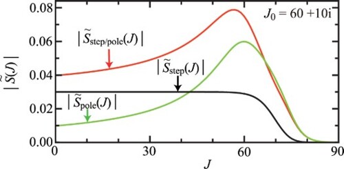
![Figure 4. S matrix data for the pole parameterisation, with J0=60+10i and a~0=1. (a) Argand diagram for s~pole(J). (b) args~pole(J)/rad versus J. (c) |s~pole(J)| versus J. (d) Θ~pole(J)/deg versus J, with 2 and 3 indicating the two branches on the F of the deflection function. Also shown as a pink dashed line and arrow are the rainbow angular momentum variable and negative rainbow angle, Jr(pole) and −θRr(pole)=−5.7∘, respectively. In (a), (b), (c), the black solid circles are for J=0(1)120, with the black arrow showing the direction of increasing J. The black solid lines are the corresponding loci. [See colour online].](/cms/asset/db3b73a9-4b9c-419a-9c7e-053da098d249/tmph_a_2198616_f0004_oc.jpg)
Figure (a) shows an Argand plot of , in which the arrow indicates the direction of increasing
. We see that
rotates clockwise, starting in the second quadrant and moves into the first quadrant as
increases from 0 to 120 in steps of unity. Figure (b) shows the corresponding plot of
versus
. We see that
decreases, corresponding to the clockwise rotation of
in Figure (a). The most rapid change in
occurs at
. For
the decrease in
approaches
. Figure (c) shows a plot of
versus
; the maximum occurs at
.
We next study the contribution of the Regge pole to . The graph of
in Figure (b) is always monotonically decreasing, which means that
is always negative, as illustrated in Figure (d). This panel illustrates two important properties:
A single pole contributes to the farside scattering.
In more detail, from Equation (Equation59(56)
(56) ), we have
(60)
(60)
Differentiation then gives a Lorentzian-type function, namely
(61)
(61) which has a minimum value of
at
. For
, the minimum is at
.
Next we examine how the above results are modified upon using a complex-valued residue, in place of unity. We have
(62)
(62)
Figure shows graphs analogous to Figure , except in Equation (Equation62(59)
(59) ) we use a partial residue of
and
for which,
. It can be seen that the effects of making
are
The starting point for the rotation of
Figure 5. S matrix data for the pole parameterisation, with and
. (a) Argand diagram for
. (b)
versus
. (c)
versus
. (d)
versus
, with 2 and 3 indicating the two branches on the F of the deflection function. Also shown as a pink dashed line and arrow are the rainbow angular momentum variable and negative rainbow angle,
and
, respectively. In (a), (b), (c), the black solid circles are for
, with the black arrow showing the direction of increasing
. The black solid lines are the corresponding loci. [See colour online].
![Figure 5. S matrix data for the pole parameterisation, with J0=60+10i and a~0=6.428+7.660i. (a) Argand diagram for s~pole(J). (b) args~pole(J)/rad versus J. (c) |s~pole(J)| versus J. (d) Θ~pole(J)/deg versus J, with 2 and 3 indicating the two branches on the F of the deflection function. Also shown as a pink dashed line and arrow are the rainbow angular momentum variable and negative rainbow angle, Jr(pole) and −θRr(pole)=−5.7∘, respectively. In (a), (b), (c), the black solid circles are for J=0(1)120, with the black arrow showing the direction of increasing J. The black solid lines are the corresponding loci. [See colour online].](/cms/asset/97576470-b8b2-463e-bc7a-dfb473b663df/tmph_a_2198616_f0005_oc.jpg)
These and other properties are readily proved using the following result for the complex numbers,
, namely, the modulus of the product equals the product of the moduli, and the argument of the product equals the sum of the arguments.
The results described above illustrate a difficulty we face when using a single Regge pole to describe rainbow scattering. The negative of the rainbow angle, , occurs at a small negative angle in the plot of
versus
– see Figure (d). For
, we found in Figures (d) and (d) that
has a minimum at
.
Now, since the minimum occurs at , one way to decrease the minimum is to use a smaller value for
. A plot of
versus
for
is shown in Figure . Comparing Figure with Figures (d) and (d), we see that the minimum is now at
, a sizable change. However, the full width at half depth of the ‘valley’ has been reduced from
in Figures (d) and (d) to only 5 partial waves in Figure , namely
, 59, 60, 61, 62. This illustrates that a single Regge pole becomes less semiclassical in its contribution to the PWS as
. We recall that a pronounced rainbow requires a contribution from many partial waves close to
if a significant rainbow is to be observed in the DCS.
Figure 6. versus
for
and
plotted as a blue solid curve. Labels 2 and 3 indicate the two branches for the F of the deflection function. Also shown as a pink dashed line and pink arrow are the rainbow angular momentum variable and negative rainbow angle,
and
, respectively. The vertical green solid lines are drawn from the
axis to approximately the full width at half depth of the ‘valley’, and show that 5 partial waves contribute, namely,
, 59, 60, 61, 62. [See colour online].
![Figure 6. Θ~pole(J)/deg versus J for J0=60+2i and a~0=1 plotted as a blue solid curve. Labels 2 and 3 indicate the two branches for the F of the deflection function. Also shown as a pink dashed line and pink arrow are the rainbow angular momentum variable and negative rainbow angle, Jr(pole) and −θRr(pole)=−28.6∘, respectively. The vertical green solid lines are drawn from the J axis to approximately the full width at half depth of the ‘valley’, and show that 5 partial waves contribute, namely, J=58, 59, 60, 61, 62. [See colour online].](/cms/asset/61cafffc-5595-484c-9731-7284bdb42887/tmph_a_2198616_f0006_oc.jpg)
8.2. Many Regge poles
When many Regge poles contribute to the scattering, Equations (59)–(61) generalise as follows, where we write with
(63)
(63) and
(64)
(64) together with
(65)
(65) To proceed further, we need information about the distribution of poles in the first quadrant of the CAM plane, together with their partial residues. Appendix considers the case where a string of poles lie on a straight line parallel to the Im
axis. We also show how the inclusion of several Regge poles can be used to make the pole-term contribution more significant, and in particular how to increase the number of partial waves affected by
in the PWS.
9. Results for DCSs including Regge poles
9.1. Introduction
In this section, we present and analyse dDCSs based on the parameterisation of Equation (Equation8(5)
(5) ). We show results for three examples: for a single pole (two examples) in the summand of Equation (Equation4
(1)
(1) ), and for a many-pole example having 6 poles. We do not discuss results already analysed in Section 7 for the smooth-step parameterisation, if the same (or similar) discussion also applies to the Regge pole case.
We want to employ a representation for based on Equations (Equation8
(5)
(5) ) and (Equation13
(10)
(10) ). However, there is now a notational ambiguity. In Equation (Equation13
(10)
(10) ),
and
are defined by the equations,
and
respectively. In the present case we have
so that
(66)
(66) We again want
and
to be defined by properties of the full deflection function, namely,
and
. This implies we have to change the notation for the phase in Equation (Equation13
(10)
(10) ). We do this by adding a prime as a label to
and
, which become
and
respectively.
To summarise, we use the following Regge pole parameterisation for the S matrix in the three examples of this section
(67)
(67) where
and
(68)
(68) with
(69)
(69) In many cases, we find,
, and,
, and if the pole sum in Equation (Equation67
(64)
(64) ) is absent, we have,
, and,
and can also replace
by unity.
We can derive a useful limiting case from Equation (Equation67(64)
(64) ), when
consists of a single term (
), and which dominates the scattering for
. i.e. the term
, is neglected. We then have from Equation (Equation66
(63)
(63) ), and using Equations (Equation68
(65)
(65) ) and (Equation69
(66)
(66) ), together with the change in notation of
→ pole [since
is absent], the result
(70)
(70) We know from Equation (Equation61
(58)
(58) ) that the minimum of the first term is
for
. Inserting
in the remaining terms gives
, so the overall result is
, or equivalently, the rainbow angle is moved to
. In this special case, the importance of the Regge pole contribution depends on the values of
and
. If
then the scattering is mainly due to the phase,
. Whereas, if
, then the scattering has contributions from both the Regge pole and
.
Our starting point for the three examples is the smooth-step parameterisation of Section 7. We know from the discussion given previously for Figures and , that this case exhibits a rainbow in its dDCS, when there is no Regge-pole sum present. By adding a pole term(s), we can examine how a Regge pole(s) affects the rainbow angular scattering.
For the three examples, we use the same seven standard parameters already employed for the smooth-step parameterisation, namely, ,
,
,
, as well as
,
,
together with
,
. We do not display the LAMs because the information they contain is consistent with the dDCS results.
9.2. Single Regge pole at
We first consider a simple example where there is a single Regge pole in the representation (67). For the partial residue, we use, . This value has been chosen so that the argument of the pole term merges smoothly with
, when the contribution from the pole term becomes significant. Our choice also ensures that the pole term makes a large contribution for
. We note the following in Figures and :
Figure (a) shows graphs of,
Properties of the full and N,F dDCSs are displayed as logarithmic plots in Figure (a–d). A comparison between the full PWS dDCS using
In Figure (b), we show the N,F PWS (r = 1) analysis of the full PWS dDCS for the angular range,
We present our SC angular distributions in Figure (c) for the angular range,
We have also applied the CoroGlo test of Section 5.2. It gives for the small-angle diffraction ratio a value of 5.3, which is not close to the forward glory ratio of 6.2. This simple test tells us that inclusion of the Regge pole term contributes to the forward angle scattering. This can also be inferred from Figure (a) where
Figure 7. S matrix data for the pole, step and step/pole ≡ s/p parameterisations. The pole parameterisation has, , and
. (a) Plots of
,
,
, versus
. (b)
versus
for the step (black dashed curve) and step/pole (red solid curve for N and blue solid curve for F) parameterisations. Also marked are,
,
,
,
, by arrows and a dashed line. The three branches of the defection functions are labelled 1 (N, red) and 2, 3 (F, both blue). (c)
versus
. [See colour online].
![Figure 7. S matrix data for the pole, step and step/pole ≡ s/p parameterisations. The pole parameterisation has, J0=60+10i, and a~0=−18.794−6.840i. (a) Plots of |S~pole(J)|, |S~step(J)|, |S~step/pole(J)|, versus J. (b) Θ~(J)/deg versus J for the step (black dashed curve) and step/pole (red solid curve for N and blue solid curve for F) parameterisations. Also marked are, Jg1, Jr, Jg2, −θRr=−44.5∘, by arrows and a dashed line. The three branches of the defection functions are labelled 1 (N, red) and 2, 3 (F, both blue). (c) (2J+1)|S~step/pole(J)| versus J. [See colour online].](/cms/asset/6ae43967-4fb8-4411-8d26-3b8baa894207/tmph_a_2198616_f0007_oc.jpg)
Figure 8. Logarithmic PWS and SC results for dDCSs, all plotted versus , for the step/pole parameterisation. The pole parameterisation has,
, and
. The pink arrows show the rainbow angle at
. (a) Full PWS dDCS for the step/pole parameterisation (black solid curve). Also shown is the full PWS dDCS for the step parameterisation (black dashed curve) in both cases for the angular range,
. (b) Full PWS dDCS (black) and PWS N(red), F(blue)
dDCSs for the angular range,
. (c) Full PWS dDCS (black) and full SC dDCS (green) for the angular range,
. (d) Full PWS and PWS N (red solid curve), F(blue solid curve)
dDCSs compared with SC N(red dashed curve, denoted SC/N/PSA), F (cyan solid curve for uAiry, and blue dashed curve for tAiry) dDCSs for the angular range,
. [See colour online].
![Figure 8. Logarithmic PWS and SC results for dDCSs, all plotted versus θR, for the step/pole parameterisation. The pole parameterisation has, J0=60+10i, and a~0=−18.794−6.840i. The pink arrows show the rainbow angle at θRr=44.5∘. (a) Full PWS dDCS for the step/pole parameterisation (black solid curve). Also shown is the full PWS dDCS for the step parameterisation (black dashed curve) in both cases for the angular range, θR=0∘−90∘. (b) Full PWS dDCS (black) and PWS N(red), F(blue) r=1 dDCSs for the angular range, θR=0∘−180∘. (c) Full PWS dDCS (black) and full SC dDCS (green) for the angular range, θR=0∘−90∘. (d) Full PWS and PWS N (red solid curve), F(blue solid curve) r=1 dDCSs compared with SC N(red dashed curve, denoted SC/N/PSA), F (cyan solid curve for uAiry, and blue dashed curve for tAiry) dDCSs for the angular range, θR=0∘−90∘. [See colour online].](/cms/asset/8a7b27d9-cd98-46eb-857c-0c5c669635bd/tmph_a_2198616_f0008_oc.jpg)
9.3. Single Regge pole at
Our second example has . The partial residue is chosen to be,
, in order to produce a smooth
curve, and to make the pole term significant for
. We note the following in Figure [properties of
,
and
] and Figure (dDCSs):
In Figure (a), we plot graphs of,
Figure (b) shows graphs of
We also see that the presence of the pole term only changes
Logarithmic plots of the full and N,F dDCSs are displayed in Figure (a–d), all for the angular range,
An important observation compared to the smooth-step result is that the position of the supernumerary rainbow has not changed much due to the addition of the Regge pole. In fact, the two curves in Figure (a) are almost indistinguishable for
In Figure (b), we show the N,F PWS (
We present our SC angular distributions in Figure (c,d). It can be seen that the full SC dDCS agrees closely (except for
The disagreement between the full SC and full PWS dDCSs at
We observe in Figure (d) that the F uAiry dDCS possesses a primary rainbow and a supernumerary rainbow at similar angles to the F PWS (
We have applied the CoroGlo test of Section 5.2. It gives for the small-angle diffraction ratio a value of 6.0, which is close to a forward glory ratio of 6.2. This tells us that inclusion of the Regge pole term contributes little to the forward angle scattering. This can also be inferred from Figure (a,b), where
Figure 9. S matrix data for the pole, step and step/pole ≡ s/p parameterisations. The pole parameterisation has, , and
. (a) Plots of
,
,
, versus
. (b)
versus
for the step (black dashed curve) and step/pole (red solid curve for N and blue solid curve for F) parameterisations. Also marked are,
,
,
,
, by arrows and a dashed line. The three branches of the deflection functions are labelled 1 (N, red) and 2, 3 (F, both blue). (c)
versus
. [See colour online].
![Figure 9. S matrix data for the pole, step and step/pole ≡ s/p parameterisations. The pole parameterisation has, J0=60+2i, and a~0=1.277−4.834i. (a) Plots of |S~pole(J)|, |S~step(J)|, |S~step/pole(J)|, versus J. (b) Θ~(J)/deg versus J for the step (black dashed curve) and step/pole (red solid curve for N and blue solid curve for F) parameterisations. Also marked are, Jg1, Jr, Jg2, −θRr=−60.7∘, by arrows and a dashed line. The three branches of the deflection functions are labelled 1 (N, red) and 2, 3 (F, both blue). (c) (2J+1)|S~step/pole(J)| versus J. [See colour online].](/cms/asset/a2916538-5476-437d-a7d6-a6eea0a7e354/tmph_a_2198616_f0009_oc.jpg)
Figure 10. Logarithmic PWS and SC results for dDCSs, for the step/pole parameterisation, all plotted versus for the angular range,
. The pole parameterisation has,
, and
. The pink arrows show the rainbow angle at
. (a) Full PWS dDCS for the step/pole parameterisation (black solid curve). Also shown is the full PWS dDCS for the step parameterisation (black dashed curve). (b) Full PWS dDCS (black) and PWS N (red), F (blue)
dDCSs. (c) Full PWS dDCS (black) and full SC dDCS (green). (d) Full PWS and PWS N (red solid curve), F (blue solid curve)
dDCSs compared with SC N (red dashed curve, denoted SC/N/PSA), F (cyan solid curve for uAiry, and blue dashed curve for tAiry) dDCSs. [See colour online].
![Figure 10. Logarithmic PWS and SC results for dDCSs, for the step/pole parameterisation, all plotted versus θR for the angular range, θR=0∘−180∘. The pole parameterisation has, J0=60+2i, and a~0=1.277−4.834i. The pink arrows show the rainbow angle at θRr=60.7∘. (a) Full PWS dDCS for the step/pole parameterisation (black solid curve). Also shown is the full PWS dDCS for the step parameterisation (black dashed curve). (b) Full PWS dDCS (black) and PWS N (red), F (blue) r=1 dDCSs. (c) Full PWS dDCS (black) and full SC dDCS (green). (d) Full PWS and PWS N (red solid curve), F (blue solid curve) r=1 dDCSs compared with SC N (red dashed curve, denoted SC/N/PSA), F (cyan solid curve for uAiry, and blue dashed curve for tAiry) dDCSs. [See colour online].](/cms/asset/cac7f5ea-a1ed-4e7e-8942-190b8193eb7f/tmph_a_2198616_f0010_oc.jpg)
9.4. Many Regge poles
Finally, in this section, we discuss our results for a parameterisation containing 6 regge poles, labelled, . We use the standard parameters as given above, but we also need to choose values for
and
. For the Regge pole positions, we use,
Note that the
are equally spaced on a straight line parallel to the
axis in the CAM plane. This case is discussed further in Appendix. The partial residues are calculated using the following equation:
(71)
(71) where
is the binomial coefficient; the corresponding numerical values for the
are reported in Table . Equation (Equation71
(68)
(68) ) can be broken into three components. The factor
is chosen so that the Regge pole contribution dominates for
. The factor,
, is used to maximise the pole contribution to
, which we have discussed in Section 8.2 and the Appendix. The remaining factor,
, is used to ensure the smoothness of
.
Table 1. Numerical values of the Regge pole positions and partial residues for n = 0, 1, 2, 3, 4, 5.
We next consider Figures and and note the following:
Figure (a–c) shows plots of
Logarithmic plots of the full and N,F dDCSs are displayed in Figure (a–d), all for the angular range,
In more detail, Figure (a) shows full PWS dDCSs constructed for the S matrix parameterisation with (black solid curve), and without (black dashed curve), Regge poles. It can be seen once more that inclusion of the poles pushes the primary rainbow to larger angles. In particular,
We show the N,F (
Our SC results are plotted in Figure (c,d). It is clear that the uAiry approximation reproduces the overall shape of the full PWS dDCS, in particular the primary plus the first and second supernumerary rainbows, although the tAiry approximation causes the NF interference oscillations to be overestimated for
The reason for these discrepancies, compared to Figure (c) for example, is that the shape of the mini-trench in Figure (b), together with its flat shoulders, means that the uAiry and tAiry approximations are less accurate.
We have applied the CoroGlo test of Section 5.2. We find for the small-angle diffraction ratio a value of 6.0, which is close to a forward glory ratio of 6.2. This tells us that inclusion of the Regge pole terms contribute little to the forward angle scattering. This can be seen in Figure (a), where the with-poles and without-poles PWS dDCSs in Figure (a) are very similar for
Figure 11. S matrix data for the pole, step and step/pole ≡ s/p parameterisations. The pole parameterisation has, for
and varying
. (a) Plots of
,
,
, versus J. (b)
versus J for the step (black dashed curve) and step/pole (red solid curve for N and blue solid curve for F) parameterisations. Also marked are,
,
,
,
, by arrows and a dashed line. The three branches of the defection functions are labelled 1 (N, red) and 2, 3 (F, both blue) (c)
versus J. [See colour online].
![Figure 11. S matrix data for the pole, step and step/pole ≡ s/p parameterisations. The pole parameterisation has, Jn=60+(10+2n)i for n=0,1,2,3,4,5 and varying a~n. (a) Plots of |S~pole(J)|, |S~step(J)|, |S~step/pole(J)|, versus J. (b) Θ~(J)/deg versus J for the step (black dashed curve) and step/pole (red solid curve for N and blue solid curve for F) parameterisations. Also marked are, Jg1, Jr, Jg2, −θRr=−87.0∘, by arrows and a dashed line. The three branches of the defection functions are labelled 1 (N, red) and 2, 3 (F, both blue) (c) (2J+1)|S~step/pole(J)| versus J. [See colour online].](/cms/asset/49bb73a9-6f3f-4001-b47b-d62d9492f7d2/tmph_a_2198616_f0011_oc.jpg)
Figure 12. Logarithmic PWS and SC results for dDCSs, for the step/pole parameterisation, all plotted versus for the angular range,
. The pole parameterisation has,
for
and varying
. The pink arrows show the rainbow angle at
. (a) Full PWS dDCS for the step/pole parameterisation (black solid curve). Also shown is the full PWS dDCS for the step parameterisation (black dashed curve). (b) Full PWS dDCS (black) and PWS N (red), F (blue)
dDCSs. (c) Full PWS dDCS (black) and full SC dDCS (green). (d) Full PWS and PWS N(red solid curve), F(blue solid curve)
dDCSs compared with SC N(red dashed curve, denoted SC/N/PSA), F (cyan solid curve for uAiry, and blue dashed curve for tAiry) dDCSs. [See colour online].
![Figure 12. Logarithmic PWS and SC results for dDCSs, for the step/pole parameterisation, all plotted versus θR for the angular range, θR=0∘−180∘. The pole parameterisation has, Jn=60+(10+2n)i for n=0,1,2,3,4,5 and varying a~n. The pink arrows show the rainbow angle at θRr=87.0∘. (a) Full PWS dDCS for the step/pole parameterisation (black solid curve). Also shown is the full PWS dDCS for the step parameterisation (black dashed curve). (b) Full PWS dDCS (black) and PWS N (red), F (blue) r=1 dDCSs. (c) Full PWS dDCS (black) and full SC dDCS (green). (d) Full PWS and PWS N(red solid curve), F(blue solid curve) r=1 dDCSs compared with SC N(red dashed curve, denoted SC/N/PSA), F (cyan solid curve for uAiry, and blue dashed curve for tAiry) dDCSs. [See colour online].](/cms/asset/eaaf12d6-9b40-4fa5-8216-0d00312eec00/tmph_a_2198616_f0012_oc.jpg)
10. Conclusions
We have incorporated, for the first time, Regge poles and residues into wHSMP for a Legendre PWS. In particular, we used pole terms of the form and then investigated their effect on the properties of the S matrix, dDCSs and LAMs. We showed results for three examples: for a single pole (two examples) and for a many-pole example having 6 poles. Our focus was on understanding the behaviour of primary and supernumerary rainbows in the product angular distributions. We began with a simple S matrix parameterisation with no Regge poles, but which exhibits a rainbow in the dDCS. We then introduced Regge poles for the three examples into the S matrix and investigated their influence on the rainbow scattering. We find that inclusion of Regge poles ‘pushes’ the rainbow angle to larger values. It is clear there is much more research that should be carried out on this topic of Regge poles in PWS. Our results are also relevant to other recent work using CAM theory and rainbows [Citation54–66].
We also analysed the scattering using Nearside-Farside (NF) PWS theory for the dDCSs and NF PWS LAM theory, including up to three resummations of the PWS. We also applied the recently introduced ‘CoroGlo’ test, which lets us distinguish between glory and corona scattering close to the forward direction. In addition, we applied full and NF asymptotic (SC) rainbow theories to the PWS – in particular, the uniform Airy and transitional Airy approximations for the farside scattering. This let us prove that structure in the no-pole and with-pole DCSs are indeed examples of primary and supernumerary rainbows, as well as the presence of other interference effects.
Disclosure statement
No potential conflict of interest was reported by the author(s).
Correction Statement
This article has been corrected with minor changes. These changes do not impact the academic content of the article.
Additional information
Funding
References
- W. Hu and G.C. Schatz, J. Chem. Phys. 125, 132301 (2006). doi:10.1063/1.2213961.
- M. Brouard and C. Vallance, editors, Tutorials in Molecular Reaction Dynamics (RSC Publishing, Cambridge, 2010).
- M.S. Child, Semiclassical Mechanics with Molecular Applications, 2nd ed. (Oxford University Press, Oxford, 2014).
- G.G. Balint-Kurti and A.P. Palov, Theory of Molecular Collisions (RSC Publishing, Cambridge, 2015). Theoretical and Computational Chemistry Series Volume 7.
- A. Laganà and G.A. Parker, Chemical Reactions: Basic Theory and Computing (Springer International Publishing, Cham, 2018).
- N.E. Henriksen and F.Y. Hansen, Theories of Molecular Reaction Dynamics: The Microscopic Foundation of Chemical Kinetics, 2nd ed. (Oxford University Press, Oxford, 2019).
- X. Shan and J.N.L. Connor, Phys. Chem. Chem. Phys. 13, 8392 (2011). doi:10.1039/C0CP01354D. This paper is referred to as H1 in the main text.
- X. Shan and J.N.L. Connor, J. Phys. Chem. A. 116, 11414 (2012). doi:10.1021/jp306435t. This paper is referred to as H2 in the main text.
- X. Shan and J.N.L. Connor, J. Phys. Chem. A. 118, 6560 (2014). doi:10.1021/jp5031762. This paper is referred to as H3 in the main text.
- X. Shan, C. Xiahou and J.N.L. Connor, Phys. Chem. Chem. Phys. 20, 819 (2018). doi:10.1039/C7CP06654F. This paper is referred to as H4 in the main text.
- C. Xiahou, X. Shan and J.N.L. Connor, Phys. Scr. 94, 065401 (2019). doi:10.1088/1402-4896/ab08b8. This paper is referred to as H5 in the main text.
- W. Heisenberg, Zeit. Phys. 120, 513–538 (1943). doi:10.1007/BF01329800. Part I. Reprinted in Werner Heisenberg, Gesammelte Werke = Collected Works, Series A, Part II, edited by W. Blum, H.-P. Dürr and H. Rechenberg, Original Scientific Papers = Wissenschaftliche Originalarbeiten (Springer-Verlag, Berlin, Germany, 1989), pp. 611–636.
- W. Heisenberg, Zeit. Phys. 120, 673–702 (1943). doi:10.1007/BF01336936. Part II. Reprinted in Werner Heisenberg, Gesammelte Werke = Collected Works, Series A, Part II, edited by W. Blum, H.-P. Dürr and H. Rechenberg, Original Scientific Papers = Wissenschaftliche Originalarbeiten (Springer-Verlag, Berlin, 1989), pp. 637–666.
- W. Heisenberg, Zeit. Phys. 123, 93–112 (1944). doi:10.1007/BF01375146. Part III. Reprinted in Werner Heisenberg, Gesammelte Werke = Collected Works, Series A, Part II, edited by W. Blum, H.-P. Dürr and H. Rechenberg, Original Scientific Papers = Wissenschaftliche Originalarbeiten (Springer-Verlag, Berlin, 1989), pp. 667–686.
- W. Heisenberg, Die Behandlung von Mehrkörperproblemen mit Hilfe der η-Matrix [Die beobachtbaren Gröβen in der Theorie der Elementarteilchen. IV]. Unpublished paper. Part IV. Reprinted in Werner Heisenberg, Gesammelte Werke = Collected Works, Series A, Part II, edited by W. Blum, H.-P. Dürr and H. Rechenberg, Original Scientific Papers = Wissenschaftliche Originalarbeiten (Berlin Germany: Springer-Verlag, 1989), pp. 687–698 (original manuscript dated 1944 by the editors).
- J.N.L. Connor, in Semiclassical Methods in Molecular Scattering and Spectroscopy, Proceedings of the NATO Advanced Study Institute held in Cambridge, England in September 1979, edited by M.S. Child (Reidel, Dordrecht, 1980), pp. 45–107.
- K.-E. Thylwe, in Resonances, the Unifying Route Towards the Formulation of Dynamical Processes. Foundations and Applications in Nuclear, Atomic and Molecular Physics, Proceedings of a Symposium held at Lertorpet, Värmland, Sweden, 1987, edited by E. Brändas and N. Elander (Springer, Berlin, 1989). Lecture Notes in Physics, 325, pp. 281–311 (1989). This review contains many Regge pole references up to 1987.
- J.N.L. Connor, J. Chem. Soc. Faraday Trans. 86, 1627 (1990). doi:10.1039/ft9908601627. This review contains many Regge pole references up to 1989.
- A.Z. Msezane, in Semiclassical and Other Methods for Understanding Molecular Collisions and Chemical Reactions, edited by S. Sen, D. Sokolovski, and J.N.L. Connor (Collaborative Computational Project on Molecular Quantum Dynamics (CCP6), Daresbury Laboratory, Warrington, 2005), pp. 95–103. ISBN 0-9545289-3-X.
- D. Sokolovski, A.Z. Msezane, Z. Felfli, S. Yu, Ovchinnikov and J.H. Macek, Nucl. Instrum. Methods Phys. Res. B. 261, 133 (2007). doi:10.1016/j.nimb.2007.04.057.
- J.N.L. Connor, J. Chem. Phys. 138, 124310 (2013). doi:10.1063/1.4794859. This paper contains many Regge pole references up to 2012.
- V. de Alfaro and T. Regge, Potential Scattering (North-Holland, Amsterdam, 1965).
- L. Castellani, A. Ceresole, R. D’Auria and P. Frè, editors, Tullio Regge: An Eclectic Genius: From Quantum Gravity to Computer Play (World Scientific, Singapore, 2020).
- J.N.L. Connor and W. Jakubetz, Mol. Phys. 35, 949 (1978). doi:10.1080/00268977800100701.
- K.-E. Thylwe and A. Amaha, Phys. Rev. A. 43, 3567 (1991). doi:10.1103/PhysRevA.43.3567.
- A. Amaha and K.-E. Thylwe, Phys. Rev. A. 50, 1420 (1994). doi:10.1103/PhysRevA.50.1420.
- P. McCabe and J.N.L. Connor, J. Chem. Phys. 104, 2297 (1996). doi:10.1063/1.470925.
- C. Xiahou, J.N.L. Connor and D.H. Zhang, Phys. Chem. Chem. Phys. 13, 12981 (2011). doi:10.1039/c1cp21044k.
- C. Xiahou and J.N.L. Connor, Phys. Chem. Chem. Phys. 16, 10095 (2014). doi:10.1039/C3CP54569E.
- C. Xiahou and J.N.L. Connor, Phys. Chem. Chem. Phys. 23, 13349 (2021). doi:10.1039/D1CP00942G.
- C. Xiahou and J.N.L. Connor, J. Phys. Chem. A. 125, 8734 (2021). doi:10.1021/acs.jpca.1c06195.
- J.N.L. Connor, P. McCabe, D. Sokolovski and G.C. Schatz, Chem. Phys. Lett. 206, 119 (1993). doi:10.1016/0009-2614(93)85527-U.
- A.J. Dobbyn, P. McCabe, J.N.L. Connor and J.F. Castillo, Phys. Chem. Chem. Phys. 1, 1115 (1999). doi:10.1039/a809498e.
- R. Anni, J.N.L. Connor and C. Noli, Phys. Rev. C: Nucl. Phys. 66, 044610 (2002). doi:10.1103/PhysRevC.66.044610.
- R. Anni, J.N.L. Connor and C. Noli, Khim. Fiz. 23 (2), 6 (2004). <https://arXiv.org/abs/physics/0410266>.
- C. Noli and J.N.L. Connor, Russ. J. Phys. Chem. 76 (Suppl. 1), S77 (2002). <https://arXiv.org/abs/physics/0301054>.
- J.N.L. Connor and R. Anni, Phys. Chem. Chem. Phys. 6, 3364 (2004). doi:10.1039/B402169J.
- J.J. Hollifield and J.N.L. Connor, Phys. Rev. A: At. Mol. Opt. Phys. 59, 1694 (1999). doi:10.1103/PhysRevA.59.1694.
- J.J. Hollifield and J.N.L. Connor, Mol. Phys. 97, 293 (1999). doi:10.1080/00268979909482830.
- A.J. Totenhofer, C. Noli and J.N.L. Connor, Phys. Chem. Chem. Phys. 12, 8772 (2010). doi:10.1039/c003374j.
- J.N.L. Connor and D.C. Mackay, Chem. Phys. 40, 11 (1979). doi:10.1016/0301-0104(79)85113-7.
- D. Sokolovski, J.F. Castillo and C. Tully, Chem. Phys. Lett. 313, 225 (1999). doi:10.1016/S0009-2614(99)01016-7.
- X. Shan and J.N.L. Connor, J. Phys. Chem. A. 120, 6317 (2016). doi:10.1021/acs.jpca.6b06028.
- J.N.L. Connor, Phys. Chem. Chem. Phys. 6, 377 (2004). doi:10.1039/b311582h.
- R.C. Fuller, Phys. Rev. C: Nucl. Phys. 12, 1561 (1975). doi:10.1103/PhysRevC.12.1561.
- J.N.L. Connor and R.A. Marcus, J. Chem. Phys. 55, 5636 (1971). doi:10.1063/1.1675732. For a commentary, see: J.N.L. Connor, Curr. Contents: Phys. Chem. Earth Sci. 31 (No. 50), 10 (1991); J.N.L. Connor, Curr. Contents: Eng., Technol. Appl. Sci. 22 (No. 50) 10 (1991). <http://garfield.library.upenn.edu/classics1991/A1991GR14400001.pdf>.
- J.N.L. Connor, Mol. Phys. 103, 1715 (2005). doi:10.1080/00268970500123576.
- C. Xiahou and J.N.L. Connor, Mol. Phys. 104, 159 (2006). doi:10.1080/00268970500314159.
- X. Shan and J.N.L. Connor, J. Chem. Phys. 136, 044315 (2012). doi:10.1063/1.3677229.
- D. Sokolovski, Chem. Phys. Lett. 370, 805 (2003). doi:10.1016/S0009-2614(03)00185-4.
- D. Sokolovski, D. De Fazio, S. Cavalli and V. Aquilanti, Phys. Chem. Chem. Phys. 9, 5664 (2007). doi:10.1039/b709427b.
- J.N.L. Connor, Mol. Phys. 31, 33 (1976). doi:10.1080/00268977600100041.
- C.A. Hobbs, J.N.L. Connor and N.P. Kirk, J. Comp. Appl. Math. 207, 192 (2007). doi:10.1016/j.cam.2006.10.079.
- D. Sokolovski and A.Z. Msezane, Phys. Rev. A: At. Mol. Opt. Phys. 70, 032710 (2004). doi:10.1103/PhysRevA.70.032710.
- D. Sokolovski, S.K. Sen, V. Aquilanti, S. Cavalli and D. De Fazio, J. Chem. Phys. 126, 084305 (2007). doi:10.1063/1.2432120.
- D. Sokolovski, D. De Fazio, S. Cavalli and V. Aquilanti, J. Chem. Phys. 126, 121101 (2007). doi:10.1063/1.2718947.
- L. Bonnet, Chin. J. Chem. Phys. 22, 210 (2009). doi:10.1088/1674-0068/22/02/210-214.
- D. Sokolovski, E. Akhmatskaya and S.K. Sen, Comput. Phys. Commun. 182, 448 (2011). doi:10.1016/j.cpc.2010.10.002.
- H. Pan and K. Liu, J. Phys. Chem. A. 120, 6712 (2016). doi:10.1021/acs.jpca.6b07772.
- N. Nešković, editor, Rainbows and Catastrophes, Proceedings of Workshop on Rainbow Scattering, Cavtat, Yugoslavia, 14–16 August 1989 (Boris Kidrić Institute of Nuclear Sciences, Belgrade, 1990).
- H. Pan, S. Liu, D.H. Zhang and K. Liu, J. Phys. Chem. Lett. 11, 9446 (2020). doi:10.1021/acs.jpclett.0c02916.
- S. Mondal, S. Bhattacharyya and K. Liu, Mol. Phys. 119, e1766706 (2021). doi:10.1080/00268976.2020.1766706.
- J.A. Adam, Phys. Rep. 356, 229 (2002). doi:10.1016/S0370-1573(01)00076-X.
- J.A. Adam, Rays, Waves and Scattering: Topics in Classical Mathematical Physics (Princeton University Press, Princeton, NJ, 2017).
- N. Nešković, S. Petrović, and M. Ćosić, editors, Rainbows in Channeling of Charged Particles in Crystals and Nanotubes, Lect. Notes Nanoscale Science and Technology, 25, chap. 1 (2017).
- C. Xiahou, X. Shan and J.N.L. Connor, J. Phys. Chem. A. 123, 10500 (2019). doi:10.1021/acs.jpca.9b07959.
Appendix
In this Appendix, we show how the inclusion of several Regge poles can be used to make the pole-term contribution more significant, in particular how to increase the number of partial waves affected by in the PWS.
We first write Equation (Equation4(1)
(1) ) in the form of a quotient
(A1)
(A1) where
= 0,1,2, … with
and
being the position and partial residue of the nth Regge pole respectively and we have written,
. It is apparent that
(A2)
(A2) and
(A3)
(A3) where
is a complex-valued function of
and
;
is a complex-valued function of
,
and
(but may be a constant, independent of
– see below).
A.1. Properties of the denominator, p()
Since is a complex number, each factor in the product defining
in Equation (A2) is itself a complex number. We can therefore separate the moduli and arguments of each factor,
, in the following way, where we use the polar form,
. We have
The contribution from to
comes purely from the phases,
. We can then write the contribution of
to
as follows
(A4)
(A4) Note the minus sign in Equation (A4); it comes from
being the denominator of
in Equation (A1).
A.1.1. Special case: the lie on a straight line parallel to the Im axis
We now consider a special case where the lie on a straight line parallel to the Im
axis in the CAM plane (n.b., not necessarily equally spaced). We write for this special case
(A5)
(A5)
Then, similar to Equation (Equation64(61)
(61) ), the phases,
, are given by
(A6)
(A6) and substituting into Equation (A4) results in
(A7)
(A7)
The minimum of Equation (A7) occurs at and has the value,
. In order to illustrate this result, we show in a plot of
versus J for 8 Regge poles, all with partial residues equal to unity, with
and
. We see the minimum of the (black) curve is at
, with the full width at half depth being
partial waves. For comparison, shows plots for the two single-Regge poles discussed in Section 8.1, namely
(green curve) and
(red curve), both with
. We see that the curve for
has a similar value for its minimum as the many-pole curve, but the ‘valley’ is much narrower (see also Figure ). In contrast, the
curve has a wider valley but a higher minimum (less negative) value [see also Figure (d)]. For the two single-pole curves, note that Equations (59)–(61) imply
.
Figure A1. versus J for (a)
and
, plotted as a red solid curve. (b)
and
, plotted as a green solid curve. (c)
for
and
, plotted as a black solid curve. Also shown as a pink dashed line and pink arrow are the rainbow angular momentum variable,
, and the corresponding angle,
, respectively. [See colour online].
![Figure A1. [−dargp(J)/dJ]/deg versus J for (a) J0=60+10i and a~0=1, plotted as a red solid curve. (b) J0=60+2i and a~0=1, plotted as a green solid curve. (c) J0=60+(10+2n)i for n=0(1)7 and a~n=1, plotted as a black solid curve. Also shown as a pink dashed line and pink arrow are the rainbow angular momentum variable, Jr(pole), and the corresponding angle, −29.2∘, respectively. [See colour online].](/cms/asset/912c92cb-0bdd-4fd2-86e7-1133570489be/tmph_a_2198616_f0013_oc.jpg)
In passing, we also note that the many-pole S matrix
can be evaluated in terms of a digamma function,
, which is the logarithmic derivative of a gamma function. For example for the 8 pole case discussed above,
we find, using Mathematica 12.1.1, that
A.2. Properties of the numerator, q()
We finally discuss the numerator, . It is defined by Equation (A3), and compared to
, is more complicated in form . It can be expressed as a polynomial in
of degree
. We can write
(A8)
(A8) Notice that the right-hand-side of Equation (A8) has
terms, and each coefficient is linear in the
. Also
depends only on
.
A.2.1. Special case: the lie on a straight line parallel to the Im axis
We now examine the conditions under which is a (complex-valued) constant, independent of
. The following relations for the coefficients must be satisfied:
(A9)
(A9) We proceed as follows. We solve the simultaneous linear equations,
in Equation (A9) for
in terms of
. The result is that
is independent of
.
Now consider the special case where the are equally spaced, lying in a straight line parallel to the
axis in the CAM plane. We can write
, and
for
, where
is the spacing. We then find that the solutions of
have an interesting property. Putting,
, the
are equal to the coefficient of the
term in the binomial expansion of the polynomial
, which is
, where the binomial coefficient is
.
For example, if we have three equally spaced Regge poles at 60 + 12i, 60 + 13i and 60 + 14i for , then the solutions of
are
and
. If we have five equally spaced Regge poles at, 60 + 10i to 60 + 14i for
, then the solutions of
are
and
. Note that the solutions are independent of the spacing, d, between each Regge pole.
If (note that the
will usually be complex valued), the solutions of
obey the following ratios:
for
.