Quantum effects of hydrogen storage in ϵ and δ semicrystalline phases of syndiotactic polystyrene through adsorption

Abstract

Syndiotactic polystyrene (sPS) is a stereoregular semicrystalline polymer which presents complex polymorphic behaviour and has been explored as an alternative for hydrogen storage using adsorption. The methodology of gas retention using a light and cheap porous material offers many advantages. To establish the adsorption capacity of a specific material, adsorption isotherms are generally measured. However, to gain a better understanding of the underlying phenomena occurring at a nanoscale level (e.g. confined interactions of ${\text{H}}_2$ in sPS) and, moreover, as a predictive tool, alternative methods such as molecular simulations are required. In this work, we present Grand Canonical Monte Carlo simulation results for hydrogen (${\text{H}}_2$) adsorption isotherms of δ and ϵ phases of sPS. ${\text{H}}_2$ molecule was described as a 1-site model with Lennard-Jones and Exp-6 potentials, within the Wigner–Kirkwood mean-field approximation to introduce quantum corrections. Both polymer phases were modelled using an atomistic force field and the initial configurations were relaxed using molecular dynamics for temperatures $T=45\text{K}$, $60\text{K}$ and $77\text{K}$. Adsorption isotherms for each system were obtained for both classical and semiclassical potentials. Additionally, adsorption isotherms for both phases were compared with experimental adsorption data at $77\text{K}$ from previous work.

GRAPHICAL ABSTRACT

Keywords:

• Hydrogen
• adsorption isotherms
• Monte Carlo
• molecular dynamics
• Wigner–Kirkwood theory

1. Introduction

Syndiotactic polystyrene (sPS) is one of the three diastereomers of polystyrene where all of the phenyl groups are positioned on alternating sides of the hydrocarbon backbone, which is not produced commercially. This order produces partially crystalline structures, giving a very rich polymorphism; until now, six crystalline structural forms have been reported. These are classified into two crystalline phase types: a trans-planar type, forming a zig-zag chain (α and β), and a helical type (γ, δ, ϵ and S−I). α and β forms are obtained via thermal annealing of a melt, meanwhile (γ, δ, ϵ and S−I form) are obtained from solute processing [1,2]. Several aspects of sPS have been investigated experimentally and using molecular simulation approach, such as structural changes when guest molecules are present, behaviour when stress is applied or a transition between phases [3–5], diffusion of guest atoms or molecules in the structure [6–8]. Pores (size and shape) play an important role in hydrogen storage [9,10] as molecule interactions are stronger in confined spaces.

Quantum effects are very noticeable under confinement since the de Broglie's thermal wavelength becomes of the order of the length size of the confinement pore and then quantum diffraction occurs, particularly at high densities, even at supercritical states not very far from the critical isotherm [11,12]. In a previous work [13], ${\text{H}}_2$ adsorption was reported for δ and ϵ sPS structures using both experimental and simulation approaches. Simulations were performed with a 3-site model for ${\text{H}}_2$, with a Lennard Jones classical potential plus a Coulomb potential contribution to mimic the quadrupole moment of hydrogen. In this work we studied adsorption of ${\text{H}}_2$ on δ and ϵ sPS structures, considering a 1-site ${\text{H}}_2$ model. The Lennard-Jones (LJ) and Buckingham's Exponential-6 (Exp-6) pair interparticle potential models were analysed. Quantum effects were introduced at the level of the Wigner–Kirkwood (WK) mean-field approach [14–17], which has been widely used to describe accurately vapour-liquid and liquid-solid phase diagrams of hydrogen and other low molecular weight substances [11,17,18], as well as adsorption isotherms of those fluids in different substrates [19,20]. The details of the force field, models and equations are described in Section 2. Results obtained in this work are presented and discussed in Section 3 for $T=45\text{K}$, $60\text{K}$ and $77\text{K}$, and the conclusions are given in Section 4.

2. Methodology

To determine adsorption isotherms of hydrogen on sPS in ϵ and δ phases, Grand Canonical Monte Carlo (GCMC) simulations at $T=45\text{K}$, $60\text{K}$ and $77\text{K}$ were performed. Bulk simulations of each value of chemical potential were carried out to obtain the relationship between pressure and chemical potential for the fluid. Each adsorption isotherm and the corresponding state point were calculated using the LJ and Exp-6 potentials, and introducing WK quantum corrections. In the following subsection, the hydrogen models are presented, explaining in Section 2.2 how the ϵ and δ structures were obtained using molecular dynamics, GCMC simulations details in Section 2.3 and adsorption isotherm calculation in Section 2.4.

2.1. Hydrogen model

Classical and semiclassical simulations were performed for a 1-site ${\text{H}}_2$ model considering LJ and Exp-6 pair potentials. The corresponding semiclassical expressions were derived according to the Wigner–Kirkwood mean-field expansion [14–17], (1) $u_{WK}(r_{ij})=u(r_{ij})+\frac{{\lambda }_B^2}{24\pi }{\mathrm{\nabla }}^{2}u(r_{ij})$(1) where $u(r_{ij})$ is a continuous potential, $u_{WK}(r_{ij})$ is the semiclassical potential energy with the Wigner–Kirkwood quantum correction and ${\lambda }_B$ is the de Broglie's thermal wavelength (${\lambda }_B=h/\sqrt{2\pi m{k}_{B}T}$, where m is the particle's mass, T temperature, h and $k_B$ are Planck's and Boltzmann's constants, respectively).

Explicit expressions of the WK pair potentials used are: (2) $\begin{array}{rl}{u}_{LJ}(r_{ij})& =4{ϵ}_{ij}[{\left(\frac{{\sigma }_{ij}}{r_{ij}}\right)}^{12}+\frac{11\pi {\lambda }_B^2}{2}{\left(\frac{{\sigma }_{ij}}{r_{ij}}\right)}^{14}\\ & -{\left(\frac{{\sigma }_{ij}}{r_{ij}}\right)}^6-\frac{5}{4}\pi {\lambda }_B^2{\left(\frac{{\sigma }_{ij}}{r_{ij}}\right)}^8]\end{array}$(2) for the LJ potential, and (3) $\begin{array}{rl}{u}_{exp6}(r_{ij})& =\frac{{ϵ}_{ij}}{(\alpha -6)}[6{\mathrm{e}}^{\alpha (1-\frac{r_{ij}}{{\sigma }_{ij}})}-\alpha {\left(\frac{{\sigma }_{ij}}{r_{ij}}\right)}^6\\ & +\frac{{\lambda }_B^2}{24\pi }(\frac{6{\alpha }^2{\mathrm{e}}^{\alpha (1-\frac{r_{ij}}{\sigma r_{ij}})}}{{\sigma }^2}\\ & -\frac{12\alpha {\mathrm{e}}^{\alpha (1-\frac{r_{ij}}{\sigma r_{ij}})}}{r_{ij}{\sigma }_{ij}}-\frac{30\alpha {\sigma }^6}{r^8})]\end{array}$(3) for the Exp-6 potential, where ${ϵ}_{ij}$ is the energy well depth between particle $\mathit{\text{i}}$ and particle $\mathit{\text{j}}$, ${\sigma }_{ij}$ is the molecular diameter and α is a dimensionless parameter. The classical limit is recovered from Equations (2(2) $\begin{array}{rl}{u}_{LJ}(r_{ij})& =4{ϵ}_{ij}[{\left(\frac{{\sigma }_{ij}}{r_{ij}}\right)}^{12}+\frac{11\pi {\lambda }_B^2}{2}{\left(\frac{{\sigma }_{ij}}{r_{ij}}\right)}^{14}\\ & -{\left(\frac{{\sigma }_{ij}}{r_{ij}}\right)}^6-\frac{5}{4}\pi {\lambda }_B^2{\left(\frac{{\sigma }_{ij}}{r_{ij}}\right)}^8]\end{array}$(2) ) and (3(3) $\begin{array}{rl}{u}_{exp6}(r_{ij})& =\frac{{ϵ}_{ij}}{(\alpha -6)}[6{\mathrm{e}}^{\alpha (1-\frac{r_{ij}}{{\sigma }_{ij}})}-\alpha {\left(\frac{{\sigma }_{ij}}{r_{ij}}\right)}^6\\ & +\frac{{\lambda }_B^2}{24\pi }(\frac{6{\alpha }^2{\mathrm{e}}^{\alpha (1-\frac{r_{ij}}{\sigma r_{ij}})}}{{\sigma }^2}\\ & -\frac{12\alpha {\mathrm{e}}^{\alpha (1-\frac{r_{ij}}{\sigma r_{ij}})}}{r_{ij}{\sigma }_{ij}}-\frac{30\alpha {\sigma }^6}{r^8})]\end{array}$(3) ) when ${\lambda }_B$ is neglected. Parameters used in this work for LJ and Exp-6 potentials are presented in Table 1.

Table 1. Non bonded parameters for LJ (Ref. [17]) and Exp-6 (Ref. [21]) potentials of hydrogen model and sPS atoms for ϵ and δ.

Potential	$ϵ({\text{kJ mol}}^{-1})$	$\sigma \text{(nm)}$	$q(e)$	α
${\text{H}}_2$ (1-site model)
${\text{LJ}}^{\mathrm{a}}$	0.3076	0.293	0.0
$\text{Exp}-6^{\mathrm{b}}$	0.3161	0.334	0.0	14.0

Note: ${}^{\mathrm{a}}$Ref. [17]

${}^{\mathrm{b}}$Ref. [21]

2.2. δ and ϵ crystalline phases

An initial box of sPS for the ϵ phase was created using the unitary cell from X-ray characterisation performed by Petraccone et al. [22]. This polymorph presents an orthorhombic structure ($\text{a}=1.62\text{nm}$, $\text{b}=2.20\text{nm}$, $\text{c}=0.79\text{nm}$) of four chains per unitary cell, with a minimum centre-to-centre distance between channels of $1.36\text{nm}$, and a density around $0.98{\text{g cm}}^{-3}$, presenting in average two channels per unitary cell. Using the same approach reported in a previous work [13], the unit cell for 6144 atoms was replicated three, two and four times in the X, Y and Z directions, respectively. The corresponding box lengths are: ${\text{L}}_x=4.86\text{nm}$, ${\text{L}}_y=4.4\text{nm}$ and ${\text{L}}_z=3.16\text{nm}$. For the δ phase, the X-ray characterisation by Chatani et al. [23] was used to generate the initial configuration with the fractional atomic coordinates. The structure corresponds to a monoclinic unitary cell: $\text{a}=1.785\text{nm}$, $\text{b}=1.326\text{nm}$, $\text{c}=0.771\text{nm}$, $\gamma ={121.2}^{\circ }$, $\text{density}=1.05{\text{g cm}}^{-3}$, two identical cavities. In this case, the unit cell was replicated three, three and four times in the X, Y and Z directions, respectively, with box lengths ${\text{L}}_x=5.35\text{nm}$, ${\text{L}}_y=3.98\text{nm}$, ${\text{L}}_z=3.08\text{nm}$ and $\gamma ={121.2}^{\circ }$. Initial structures are presented in Figure 1 for both phases:

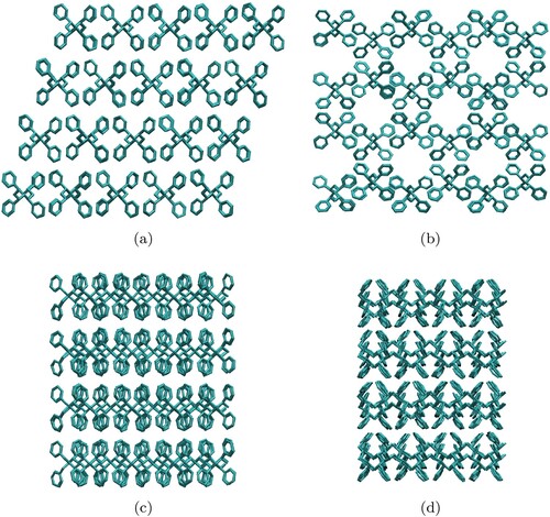
Figure 1. Snapshots of initial configurations taken from X-ray characterisation for (a), (c) δ and (b), (d) ϵ phase structures: (a), (b) are the projections along the a axis, (c), (d) represent the projection along the c axis.

Once the ϵ and δ initial structures were generated, NVT and NPT molecular dynamic (MD) simulations were obtained with GROMACS 2021.6 [24]. Three temperatures were used: 45, 60 and $77\text{K}$, and a pressure $P=0.1\text{MPa}$. MD simulations were performed with a force field fitted to simulate benzene-polystyrene systems [25]. Non-bonded and bonded parameters for polystyrene atoms can be found in Table 1. These parameters were taken from [25]. LJ and Exp-6 non-bonded parameters for ${\text{H}}_2$ molecules can be found in Table 2. Cross parameters between sPS atoms and ${\text{H}}_2$ molecules were calculated using the Lorentz-Berthelot (LB) combining rules. Although the molecular parameters used to obtain the corresponding values for the cross-interaction belong to different potentials, an equivalent procedure has been followed in the case of the family of Mie potentials, which are Lennard-Jones interactions with different values of the repulsive and attractive exponents n and m. By changing these exponents, the potentials are modified, and the systems are described as non-conformal since can not be mapped between them by a change of energy and spatial scales. In consequence, the thermodynamic properties do not follow corresponding states. One of the first studies about the LB rules for non-conformal potentials was reported by Calvin and Reed [26] and is a standard procedure in the applications of the SAFT-VR-Mie approach (see [27]). A more detailed discussion is given in the supplementary information.

Table 2. Non-bonded and bonded LJ parameters for sPS atoms (δ and ϵ phases). ${\text{C}}_{al}$ and ${\text{H}}_{al}$ represent aliphatic carbon and hydrogen, meanwhile ${\text{C}}_{ar}$ and ${\text{H}}_{ar}$ represent aromatic carbon and hydrogen respectively. The force field for sPS was derived in a previous work [25].

Atom	$ϵ({\text{kJ mol}}^{-1})$	$\sigma \text{(nm)}$	$q(e)$
C (aliphatic)	0.3519	0.3207	0.0
C (aromatic)	0.294	0.355	-0.115
H (aliphatic)	0.318	0.2318	0.0
H (aromatic)	0.126	0.242	+0.115
Bond	Distance (nm)
${\text{C}}_{al}$-${\text{C}}_{al}$	0.153
${\text{C}}_{al}$-${\text{H}}_{al}$	0.110
${\text{C}}_{ar}$-${\text{C}}_{al}$	0.139
${\text{C}}_{ar}$-${\text{H}}_{ar}$	0.108
${\text{C}}_{al}$-${\text{C}}_{ar}$	0.151
	$V(\varphi )=(k_{\varphi }/2)(\varphi -{\varphi }_0{)}^2$
Bond angles	${\varphi }_0\text{(deg)}$	$k_{\varphi }({\text{kJ mol}}^{-1}{\text{rad}}^{-2})$
H-$C_{al}$-H	109.45	306.4
${\text{C}}_{al}$-${\text{C}}_{al}$-H	109.45	366.9
${\text{C}}_{al}$-${\text{C}}_{al}$-${\text{C}}_{al}$	109.45	482.3
${\text{C}}_{ar}$-${\text{C}}_{al}$-H	109.45	366.9
${\text{C}}_{al}$-${\text{C}}_{al}$-${\text{C}}_{ar}$	109.45	482.3
${\text{C}}_{al}$-${\text{C}}_{ar}$-${\text{C}}_{ar}$	120.00	376.6
${\text{C}}_{ar}$-${\text{C}}_{ar}$-${\text{C}}_{ar}$	120.00	376.6
${\text{C}}_{ar}$-${\text{C}}_{ar}$-H	120.00	418.8
	$V(\tau )=(k_{\tau }/2)[1-\cos 3(\tau -{\tau }_0)]$, cis at $0^{\circ }$
Dihedral angles	${\tau }_0\text{(deg)}$	$k_{\tau }({\text{kJ mol}}^{-1})$
${\text{C}}_{al}$-${\text{C}}_{al}$-${\text{C}}_{al}$-${\text{C}}_{al}$	180.0	12.0
${\text{C}}_{al}$-${\text{C}}_{al}$-${\text{C}}_{al}$-H (terminal methyl)	180.0	12.0
	$V(\delta )=(k_{\delta }/2)(\delta -{\delta }_0{)}^2$, cis at $0^{\circ }$
Harmonic dihedral angles	${\delta }_0$ (deg)	$k_{\delta }({\text{kJ mol}}^{-1})$
${\text{C}}_{ar}$-${\text{C}}_{ar}$-${\text{C}}_{ar}$-${\text{C}}_{ar}$	0.0	167.4
$\text{C}{2}_{ar}$-$\text{C}{3}_{ar}$-$\text{C}{1}_{ar}$-H [on C2]	0.0	167.4
$\text{C}{2}_{ar}$-$\text{C}{3}_{ar}$-$\text{C}{1}_{ar}$-${\text{C}}_{al}$ [on C2]	0.0	167.4

In NVT simulations, a V-rescale thermostat [28] for equilibration was employed, with a simulation length time of $5\text{ns}$ (timestep $dt=0.002\text{ps}$), and a coupling parameter of ${\tau }_T=0.5$. For NPT runs the same parameters as in NVT simulations were applied, adding a C-rescale barostat [29] with a coupling parameter of ${\tau }_P=2.0$, as this barostat can be applied for both equilibration and sampling steps. The final configuration from NPT runs was used as the adsorbent material in the GCMC simulations. Box dimensions for each final configuration of MD runs are presented in Table 3.

2.3. GCMC simulations

GCMC simulations were performed for ${\text{H}}_2$ in bulk and confined phases. In the first case, the total chemical potential ${\mu }^T$ given by the sum of the ideal and excess contributions, ${\mu }^{IG}$ and ${\mu }^{Ex}$ respectively, was fixed at different values along the isotherm, and the pressure was calculated using the virial theorem. The goals for doing these simulations were to check the performance of the LJ and Exp-6 potentials when compared with experimental data, and also to obtain the relationship between pressure and chemical potential. In the confined systems, the final configurations of the previously equilibrated sPS structures were taken to calculate the hydrogen adsorption isotherms. These structures were kept static during the Monte Carlo simulations.

Table 3. Final size of each simulation box after molecular dynamics equilibration. Dimensions L${}_x$,L${}_y$,L${}_z$, solid volume $V_S$ and solid density ${\rho }_S$ are reported.

$T\text{(K)}$	$L_X\text{(nm)}$	$L_Y\text{(nm)}$	$L_Z\text{(nm)}$	$V_S({\text{m}}^{-3})$	${\rho }_S({\text{kg m}}^{-3})$
δ structure
45	5.1798	4.1118	3.0783	65.563	1012.96
60	5.1857	4.1165	3.0818	65.787	1009.50
77	5.1896	4.119	3.0841	65.926	1007.24
ϵ structure
45	4.7677	4.3164	3.0999	63.794	1041.02
60	4.7734	4.3216	3.1037	64.025	1037.27
77	4.7779	4.3257	3.1066	64.206	1034.35

Each MC cycle consisted of N translations, and $100\text{N}$ creation/removal of a particle, where N is the number of molecules in the simulation box. After $5\times {10}^4$ cycles for equilibration, $5\times {10}^4$ cycles were required for averaging with a block size of 1000 cycles.

2.4. Adsorption isotherms

To avoid ambiguities, it is important to define the considered system clearly. Most of the following definitions were taken partially from Reference [30]. The crystalline structures used for MC calculations were obtained after relaxation and equilibration performed by MD calculations at the different temperatures of interest. The adsorbate is in contact with an infinite reservoir of fluid in the bulk phase at constant temperature and constant chemical potential (or pressure). The whole volume of the adsorbate $V_S$ is fixed, and it is comprised of the solid part and the empty space of the pores. The total number of moles in the system is: (4) $n_T=n_{ads}+n_S$(4) where $n_{ads}$ are the moles of adsorbate and $n_S$ the moles of the solid. The absolute adsorption (obtained directly from GCMC simulations) is given when the moles of the solid are removed: (5) $n^{abs}=n_T-n_S=n_{ads}$(5) To calculate net adsorption, the moles contained in a fluid at the same pressure and temperature of the system are subtracted from the absolute adsorption: (6) $n^{net}(\mu ,T)=n^{abs}(\mu ,T)-n^{bulk}(\mu ,T)$(6) If we divide Equation (6(6) $n^{net}(\mu ,T)=n^{abs}(\mu ,T)-n^{bulk}(\mu ,T)$(6) ) by $V_S$, the following expression is obtained (7) $\frac{n^{net}}{V_S}={\mathrm{\Gamma }}^{net}(\mu ,T)={\mathrm{\Gamma }}^{abs}(\mu ,T)-{\mathrm{\Gamma }}^{bulk}(\mu ,T)$(7) where ${\mathrm{\Gamma }}^{bulk}$ is the molar density, obtained by running a GCMC simulation in a box of volume V at T and μ employing the following relation: (8) ${\mathrm{\Gamma }}^{bulk}(\mu ,T)=\frac{⟨n(\mu ,T)⟩}{V}$(8) The corresponding pressures were obtained from the same simulations using the virial equation for pressure [31].

The adsorption isotherms presented in the Results section were represented in mass/mass percentage. These are the units generally used by many experimentalists in hydrogen storage. To calculate it, the next relations were employed: (9) $\begin{array}{rl}\mathit{\text{Total amount adsorbed (wt \%)}}& =\frac{{\mathrm{\Gamma }}^{abs}{M}_{H_2}}{{\rho }_S}\ast 100\end{array}$(9) (10) $\begin{array}{rl}& \mathit{\text{Net amount adsorbed (wt\%)}}\\ & =\frac{M_{H_2}({\mathrm{\Gamma }}^{abs}-{\mathrm{\Gamma }}^{bulk})}{{\rho }_S}\ast 100\\ & =\frac{M_{H_2}{\mathrm{\Gamma }}^{net}}{{\rho }_S}\ast 100\end{array}$(10) where $M_{H_2}$ is the molecular weight of hydrogen in $gmo{l}^{-1}$ and ${\rho }_S=\frac{m_S}{V_S}$ is the solid density in $g{m}^{-3}$. Solid density values for each system can be found in Table 3.

3. Results and discussion

Performance of the potential models was studied first in bulk phase, i.e. no sPS adsorbent was present. Low temperatures for ${\text{H}}_2$ were considered, with pressures ranging from $P=0.05\text{MPa}$ to 10 MPa, modifying the chemical potential accordingly in each simulation point. As observed in Figure 2, the classical and semiclassical potentials agree very well with experimental data for temperature $T=45\text{K}$ and low pressures below $P=1.5\text{MPa}$. This data was obtained using the database REFPROP [32]. However, at higher pressures, both classical potentials tend to overestimate the experimental density, whereas the semiclassical WK models give very accurate predictions, even for very high pressures, $P=10\text{MPa}$. This behaviour is expected since quantum effects should be evident at low temperatures and high pressures, whereas classical potentials do not include quantum effects.

Figure 2. Density (ρ) vs. pressure (P) plot for ${\text{H}}_2$ in bulk phase at $T=45\text{K}$ in linear (left) and semi-log (right) scale. Symbols represent data obtained by GCMC simulations for each intermolecular potential (circles for LJ, triangles down for LJ-3 sites model, squares for LJ-WK, triangles for Exp-6 and diamonds for Exp-6-WK). Dashed lines are only a visual guide. Solid line represents experimental data retrieved from REFPROP [32].

For $T=60\text{K}$ (Figure 3), the calculated densities using GCMC simulations (classical and semiclassical potentials) agree with the experimental data reported up to a pressure $P=2.0\text{MPa}$. At higher pressures, the densities calculated by adding quantum corrections agree with the experimental densities; meanwhile, the curve obtained from classic potentials deviates significantly as pressure increases. However, this deviation from experimental densities is smaller than the one observed in the previous temperature ($T=45\text{K}$), which agrees with the fact that quantum effects become more relevant at lower temperatures. As the temperature increases, the de Broglie thermal wavelength ${\lambda }_B$ decreases, implying a lower contribution of quantum effects.

Figure 3. ρ vs. P plot for ${\text{H}}_2$ in bulk phase at $T=60\text{K}$ in linear (left) and semi-log (right) scale. Symbols represent data obtained by GCMC simulations for each intermolecular potential (circles for LJ, triangles down for LJ-3 sites model, squares for LJ-WK, triangles for Exp-6 and diamonds for Exp-6-WK). Dashed lines are only a visual guide. Solid line represents experimental data retrieved from REFPROP [32].

The density obtained for temperature $T=77\text{K}$ for the classical and WK models is presented in Figure 4, In both cases there is agreement with experimental data but deviations are noticeable at high pressures, $P=5.0\text{MPa}$, where the classical potentials also overestimate density with respect to semiclassical potentials. It is important to remark that a 1-site hydrogen model (no charges present) agrees with experimental data and deviations at low temperatures are greatly reduced when adding a quantum correction term to the classical potentials.

Figure 4. ρ vs. P plot for ${\text{H}}_2$ in bulk phase at $T=77\text{K}$ in linear (left) and semi-log (right) scale. Symbols represent data obtained by GCMC simulations for each intermolecular potential (circles for LJ, triangles down for LJ-3 sites model, squares for LJ-WK, triangles for Exp-6 and diamonds for Exp-6-WK). Dashed lines are only a visual guide. Solid line represents experimental data retrieved from REFPROP [32].

As mentioned in Section 2, bulk simulations allow us to relate density, chemical potential and pressure for every temperature that is required to calculate adsorption isotherms for ${\text{H}}_2$ confined in δ and ϵ phases. Moreover, quantum effects in ${\text{H}}_2$ bulk system can be analysed, which seems to be relevant even at $T=77\text{K}$.

For sPS systems, both structures at different temperatures were analysed, at the same chemical potentials and corresponding pressures used in bulk simulations. Figure 5 compares adsorption isotherms for each potential at $T=45\text{K}$ for δ and ϵ structures. Figure 5a and c present the total amount adsorbed in sPS structures, calculated by Equation (9(9) $\begin{array}{rl}\mathit{\text{Total amount adsorbed (wt \%)}}& =\frac{{\mathrm{\Gamma }}^{abs}{M}_{H_2}}{{\rho }_S}\ast 100\end{array}$(9) ). Figure 5b and d give the net amount adsorbed, calculated by Equation (10(10) $\begin{array}{rl}& \mathit{\text{Net amount adsorbed (wt\%)}}\\ & =\frac{M_{H_2}({\mathrm{\Gamma }}^{abs}-{\mathrm{\Gamma }}^{bulk})}{{\rho }_S}\ast 100\\ & =\frac{M_{H_2}{\mathrm{\Gamma }}^{net}}{{\rho }_S}\ast 100\end{array}$(10) ). As it is observed in Figure 5a, the adsorption calculated using the Exp-6 potential is noticeably higher than the one calculated using the other potentials. It is expected that classic potentials tend to have higher adsorption than semiclassical ones, as it is known that the inclusion of quantum corrections introduces a higher value of the effective diameter, that at low densities goes as ${\sigma }_{eff}\approx \sigma +{\lambda }_B/2\sqrt{2}$ [33]. This effective diameter reduces the available adsorption volume since the excluded volume increases with respect to the classical model, an effect that we have reported previously for a semiclassical thermodynamic perturbation theory model for square-well particles [18]. In Figure 5a it is possible to note that, for δ phase, the sPS saturates approximately at $P=0.2\text{MPa}$ for LJ and Exp-6-WK potentials. For the Exp-6 and LJ-WK models, adsorption isotherms saturate approximately at $P=1.5\text{MPa}$. In Figure 5b, we observe a maximum of net adsorption at very low pressure, $P<0.1\text{MPa}$ for all potentials.

Figure 5. Adsorption isotherms of ${\text{H}}_2$ in sPS at $T=45\text{K}$ for LJ, LJ-WK, Exp-6 and Exp-6-WK potentials calculated by GCMC simulations. Figure (a) and (b) present total adsorption and net adsorption isotherms of ${\text{H}}_2$ (in percentage) respectively, for δ phase. Figure (c) and (d) present total adsorption and net adsorption isotherms of ${\text{H}}_2$ (in percentage) respectively, for the ϵ phase.

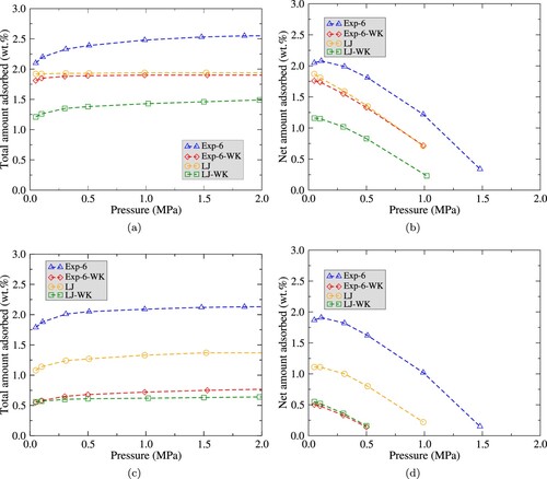
For the ϵ phase, values for adsorption have a significant variation for each potential, as observed in Figure 5c. LJ and Exp-6 systems predict higher adsorption with respect to the semiclassical fluids. The adsorption isotherms saturate at lower pressures when the quantum correction is applied ($0.5\text{MPa}$). As in the δ phase, net adsorption is at a maximum in pressures not greater than $0.1\text{MPa}$ for all potentials (see Figure 5d).

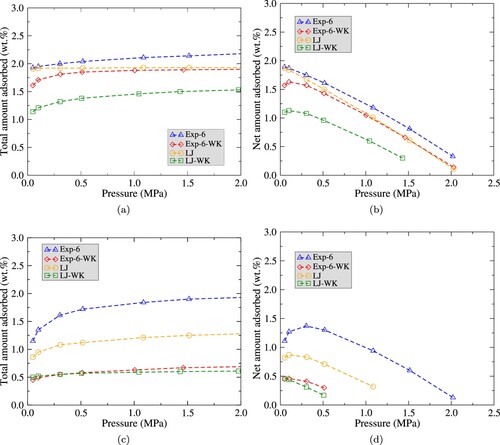
Adsorption at temperature $T=60\text{K}$ continues to be higher when the classical models are used. The LJ-WK potential predicts the lowest adsorption in the sPS structure. This is also an expected behaviour, thus the prediction for ${\text{H}}_2$ packing in δ cavities is lower than for the Exp6-WK model.

Adsorption of ${\text{H}}_2$ in these conditions saturates at pressure $P=2.0\text{MPa}$ for both WK potential models, $P<0.1\text{MPa}$ and $P=1\text{MPa}$ for the LJ and Exp-6 models, respectively, see Figure 6a. In the case of the δ phase, the maximum net adsorption is presented at very low pressures, basically $P<0.1\text{MPa}$ for all the potential models, similarly to what occurs at temperature $T=45\text{K}$, as observed in Figure 6b. For the ϵ structure a lower adsorption for all the potential models is obtained when compared with the δ phase, see Figure 6c. In this case, the saturation range in pressure is $1.0\text{MPa}<P<1.5\text{MPa}$, with the maximum net adsorption values at pressures below $0.1\text{MPa}$ for the LJ model and both WK systems, whereas $P=0.3\text{MPa}$ for the classical Exp-6 (see Figure 6d).

Figure 6. Adsorption isotherms of ${\text{H}}_2$ on sPS at $T=60\text{K}$ for LJ, LJ-WK, Exp-6 and Exp-6-WK potentials calculated by GCMC simulations. Figure (a) and (b) present total adsorption and net adsorption isotherms of ${\text{H}}_2$ (in percentage) respectively, for δ phase. Figure (c) and (d) present total adsorption and net adsorption isotherms of ${\text{H}}_2$ (in percentage) respectively, for the ϵ phase.

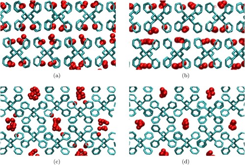
A relevant feature comparing the adsorption isotherms for the sPS structures are very similar for both WK potential models, whereas for the δ structure they are very well differentiated. A plausible physical explanation for this is that the cavities and channels present in the δ and ϵ phases, respectively, give different response for different potential models. ${\text{H}}_2$ molecules are closer each other in cavities than in channels, as can be seen in Figure 7 for the LJ and LJ-WK models. The effective higher molecule predicted by the quantum correction modifies the ${\text{H}}_2$ adsorption, as also predicted in a previous theoretical work for adsorption of ${\text{H}}_2$ onto carbon-based structures [18]. Comparing Figure 7a and b we observe that LJ-WK molecules are more packed in the cavities of the δ phase when compared to the corresponding classical model. The same occurs for the channels in the ϵ phase, see Figure 7c and d.

Figure 7. Snapshots of final GCMC configurations at $T=60\text{K}$ for (a) δ phase LJ potential, (b), δ phase LJ-WK potential, (c) ϵ phase LJ potential and (d) ϵ phase LJ-WK potential, using projections along the a axis in each snapshot.

Adsorption isotherms for temperature $T=77\text{K}$ are presented in Figure 8. A rough comparison in both crystalline phases with experimental adsorption isotherms [13] is given. Due to the nature of the material, with amorphous and crystalline conformations, it is not possible to do a direct comparison with experimental data, since the experimental adsorption isotherms were obtained by subtracting from the total amount adsorbed in both phases the adsorption on the dense β sPS phase at temperature $T=77\text{K}$. All the sPS semi-crystalline materials were prepared as aerogels of the same nano fibrillar morphology, with a 35-40 % degree of crystallinity and with the same range of porosity, 88-95 %.

Figure 8. Adsorption isotherms of ${\text{H}}_2$ in sPS at $T=77\text{K}$ for LJ, LJ-WK, Exp-6 and Exp-6-WK potentials calculated by GCMC simulations. Figure (a) and (b) present total adsorption and net adsorption isotherms of ${\text{H}}_2$ (in percentage) respectively, for δ phase. Figure (c) and (d) are total adsorption and net adsorption isotherms of ${\text{H}}_2$ (in percentage) respectively, for the ϵ phase. In Figure (a) and (c), also experimental (solid line) and simulation (cross symbols) values from a previous work [13] are plotted.

The adsorption on the β phase is due to the amorphous part because the crystalline part has a very high packing and is without space to adsorb hydrogen. A more detailed explanation of these experiments can be found elsewhere in Ref. [13], Figures 2 and 9. In this previous work, simulations were also developed but a different model was used; a 3-site hydrogen model with explicit Coulomb's charges. Experimental data was measured for both structures up to a pressure $P=1.75\text{MPa}$. In Figure 8a, the potentials used in this work present higher adsorption than the 3-site hydrogen model. The LJ-WK potential curve seems to follow better the experimental data for δ phase at low pressures ($P<2.0\text{MPa}$). Classic potentials have a very similar adsorption behaviour. Figure 8b indicates maximum net adsorption at $P=0.3\text{MPa}$ for Exp-6-WK potential and $P<0.1\text{MPa}$ for other potentials.

In Figure 8c we can observe that the WK models give a better prediction of the low pressures adsorption isotherms, up to $P=1.0\text{MPa}$ and particularly for the Exp-6 potential. Using semiclassical potentials for the ϵ phase does predict the saturation at $P=0.5\text{MPa}$ and classical potentials do allow more adsorption, saturating approximately at $P=1.5\text{MPa}$. In Figure 8d, the maximum net adsorption is observed at $P=0.5\text{MPa}$ for Exp-6 potential and $P<0.1\text{MPa}$ for the other potentials. It is relevant to note that, even at $T=77\text{K}$ where bulk simulations do not present a significant difference between potentials (up to $P=5.0\text{MPa}$), adsorption isotherms in sPS structures do change for all potentials. Also, in the δ phase, differences between LJ-WK and Exp-6-WK are noticeable at each temperature; however, for the ϵ phase, adsorption isotherms tend to have similar values as temperature increases.

4. Conclusions

In this work we have presented the relevance of introducing quantum effects in order to describe adsorption isotherms of ${\text{H}}_2$ in δ and ϵ phases of sPS. Using 1-site model classical simulations for ${\text{H}}_2$ in bulk phases can reproduce experimental data only at low pressures, $P<2.0\text{MPa}$, whereas the Wigner–Kirkwood mean-field semiclassical potentials can be used even for pressures as high as $10\text{MPa}$. For ${\text{H}}_2$ in syndiotactic polystyrene (sPS) structure, adsorption is higher on δ phase than ϵ phase for temperatures T=45, 60 and $77\text{K}$. For these isotherms, the difference between LJ and Exp-6 potential are more notable in δ phase than ϵ phase. As already mentioned before, these differences could be consequence of the different pore morphology in the δ and ϵ phases, since stronger confinement is present in the ϵ structure, and then the differences between potentials must be more noticeable, particularly when quantum corrections are introduced. More experimental data of ${\text{H}}_2$ adsorption isotherms at lower temperatures ($T=45\text{K}$ and $60\text{K}$) in a wider range of pressures for these sPS structures are required to determine which potential has a better prediction. Experimental data at $T=77\text{K}$ suggests that, for both δ and ϵ phases, a 1-site ${\text{H}}_2$ model using a LJ-WK potential could perform a reasonable prediction of ${\text{H}}_2$ adsorption at low pressures ($P<1\text{MPa}$), followed by Exp-6-WK potential. Finally, for each temperature studied in this work, adsorption isotherms for classical potentials tend to be higher than their semiclassical counterparts.

Disclosure statement

No potential conflict of interest was reported by the author(s).

Additional information

Funding

We acknowledge support from the University of Guanajuato, Dirección de Investigación y Posgrado (grant CIIC 151/2022 and 250/2023). Also, we gratefully acknowledge the computing time granted by LANCAD/CONACyT on the supercomputer Miztli at DGTIC UNAM. We thank CONACyT for Kevin R. Arriola Gonzalez's PhD scholarship, number 819666.

References

- Y. Tamai, Polymer 128, 177–187 (2017). doi:10.1016/j.polymer.2017.09.028
- C. Liu, K. Kremer and T. Bereau, Adv. Theory Simul. 1 (7), 1800024 (2018). doi:10.1002/adts.v1.7
- Y. Tamai and M. Fukuda, J. Chem. Phys. 121 (23), 12085–12093 (2004). doi:10.1063/1.1815292
- E.B. Gowd, K. Tashiro and C. Ramesh, Prog. Polym. Sci. 34 (3), 280–315 (2009). doi:10.1016/j.progpolymsci.2008.11.002
- Y. Tamai, ACS. Macro. Lett. 2 (9), 834–838 (2013). doi:10.1021/mz400386z PMID: 35606990.
- G. Milano, G. Guerra and F. Müller-Plathe, Chem. Mater. 14 (7), 2977–2982 (2002). doi:10.1021/cm011297i
- S. Asahi and Y. Tamai, Mol. Simul. 41 (10-12), 974–979 (2015). doi:10.1080/08927022.2014.930571
- Y. Tamai, J. Memb. Sci. 646, 120202 (2022). doi:10.1016/j.memsci.2021.120202
- Z.Y. Zhang, X.H. Liu and H. Li, Int. J. Hydrogen. Energy. 42 (7), 4252–4258 (2017). doi:10.1016/j.ijhydene.2016.10.077
- D. Caviedes and I. Cabria, Int. J. Hydrogen. Energy. 47 (23), 11916–11928 (2022). doi:10.1016/j.ijhydene.2022.01.229
- V.M. Trejos, A. Gil-Villegas and A. Martinez, J. Chem. Phys. 139 (18), 184505 (2013). doi:10.1063/1.4829769
- A. Helmi and Z. Vosoughi, Fluid. Phase. Equilib. 491, 24–34 (2019). doi:10.1016/j.fluid.2019.02.026
- S. Figueroa-Gerstenmaier, C. Daniel, G. Milano, J.G. Vitillo, O. Zavorotynska, G. Spoto and G. Guerra, Macromolecules 43 (20), 8594–8601 (2010). doi:10.1021/ma101218q
- E. Wigner, Phys. Rev. 40 (5), 749–759 (1932). doi:10.1103/PhysRev.40.749
- J.G. Kirkwood, Phys. Rev. 44 (1),31–37 (1933). doi:10.1103/PhysRev.44.31
- R.M. Stratt, J. Chem. Phys. 72 (3), 1685–1688 (1980). doi:10.1063/1.439278
- Y. Rosenfeld, J. Chem. Phys. 73 (11), 5760–5765 (1980). doi:10.1063/1.440058
- V.M. Trejos, M. Becerra, S. Figueroa-Gerstenmaier and A. Gil-Villegas, Mol. Phys. 112 (17), 2330–2338 (2014). doi:10.1080/00268976.2014.903591
- E.D. Glandt, J. Chem. Phys. 74 (2), 1321–1325 (1981). doi:10.1063/1.441193
- V.M. Trejos, A. Martínez and A. Gil-Villegas, Fluid. Phase. Equilib. 462, 153–171 (2018). doi:10.1016/j.fluid.2018.01.028
- J.A. Krumhansl and S.Y. Wu, Phys. Rev. B 5 (10), 4155–4170 (1972). doi:10.1103/PhysRevB.5.4155
- V. Petraccone, O. Ruiz de Ballesteros, O. Tarallo, P. Rizzo and G. Guerra, Chem. Mater. 20 (11), 3663–3668 (2008). doi:10.1021/cm800462h
- Y. Chatani, Y. Shimane, T. Inagaki, T. Ijitsu, T. Yukinari and H. Shikuma, Polymer 34 (8), 1620–1624 (1993). doi:10.1016/0032-3861(93)90318-5
- Lindahl, Abraham, Hess and van der Spoel 2022. doi:10.5281/zenodo.6801839
- F. Müller-Plathe, Chem. Phys. Lett. 252 (5-6), 419–424 (1996). doi:10.1016/0009-2614(96)00169-8
- D.W. Calvin, I. Reed and T.M. Reed, J. Chem. Phys. 54 (9), 3733–3738 (2003). doi:10.1063/1.1675422
- C.C. Walker, J. Genzer and E.E. Santiso, J. Chem. Phys. 152 (4), 044903 (2020). doi:10.1063/1.5126213
- G. Bussi, D. Donadio and M. Parrinello, J. Chem. Phys. 126 (1), 014101 (2007). doi:10.1063/1.2408420
- M. Bernetti and G. Bussi, J. Chem. Phys. 153 (11), 114107 (2020). doi:10.1063/5.0020514
- S. Brandani, E. Mangano and L. Sarkisov, Adsorption 22 (2), 261–276 (2016). doi:10.1007/s10450-016-9766-0
- D. Frenkel and B. Smit, Understanding Molecular Simulation: From Algorithms to Applications (Computational Science Series, Vol 1), hardcover ed. (2001), p. 664.
- E.W. Lemmon, M.L. Huber and M.O. McLinden, NIST Standard Reference Database 23: Reference Fluid Thermodynamic and Transport Properties – REFPROP, National Institute of Standards and Technology, Standard Reference Data Program, Gaithersburg, 9th ed. 2010.
- B. Yoon and H.A. Scheraga, J. Chem. Phys. 88 (6), 3923–3933 (1988). doi:10.1063/1.453841