A discussion on the properties of the simultaneous triple-valued function whose job is to fit the PESs with triply and doubly degenerate seams together

Abstract

In the previous work, a novel and yet complicated mathematical model to predict the presence of triply degenerate seam was presented and was illustrated its efficiency using some physical models. Here in this work, a discussion on the ability of the model to account for the cusping features found in the potential energy surfaces (PESs) is presented in addition to a discussion on the derivatives and its discontinuities and infiniteness at a specific point. Analytical evaluation of derivatives is possible in principle but in practice, numerical approximation to the exact derivatives is the only way out to solve this problem. Two examples (one being physical and the other being the chemically realistic) are considered to probe the above-mentioned properties of the simultaneous model. The integration of the model function gives finite values everywhere disregarding the presence and absence of degeneracy. This is just opposite to derivative evaluation. A noteworthy point is that the analytical model fits everywhere equally well all over the topography of PESs including the vicinity of seam. This quality makes the model an ideal choice for modelling purpose.

GRAPHICAL ABSTRACT

Keywords:

• Potential energy surface
• adiabatic/diabatic transformation
• analytical model potential energy
• triple degeneracy
• conical intersection
• mixing angle

1. Introduction

The concept of triply degenerate point is chronologically new one, formed from the simultaneous intersection of three surfaces at a given point and can either be an isolated feature confined to a certain region of space, especially in a low symmetric molecule or be a continuous seam guided by symmetry in spherically degenerate molecules. The first ever reporting of such a triply degenerate point appeared in early eighties [1]. The triple point has the potential to display an anomalous behaviour in the spectroscopy of excited states and has profound implications in photo physics, chemistry and biology. Its ab-initio characterisation and dynamics revealing the competitive pathways among the probables were done as recently as the beginning of 2000 [2–13]. In spherically symmetric molecular system, seam associated with the triple point is well demanded by the group theoretical considerations as the many fold degeneracies among the states keeps on increasing with the increasing order of the point group. On the other hand, in the less symmetric molecule, the existence of such a seam or an isolated point is not a direct consequence of symmetric considerations alone as there are only non-degenerate states but rather an accidental crossing of states of either same or different symmetries.

These seams (mainly not required by symmetry) were identified and characterised via ab-initio calculations in low symmetric molecules, particularly the organic and biochemical ones. In the literature, there have been many instances of such molecules reported to possess the triple point [14–16]. An algorithm was claimed to have developed to optimise the seam of triple degeneracy to locate an optimised CI/cusp geometry within the desirable accuracy based on quantum mechanics and molecular mechanics method and was applied to pyrazine, thiophene,cytosine,manoladehyde, etc. [4–6, 9, 17, 18]. For the two state problem, this type of algorithm already exists in commercial software packages [19–21]. Two state conical intersections in molecules were modelled via the set of analytical eigen-valued expressions (two of them, Equation 1b(1b) $\begin{array}{rl}{V}_{\pm }& =\frac{V_{11}+V_{22}}{2}\pm \frac{1}{2}\sqrt{(V_{11}-V_{22}{)}^2+4|V_{12}{|}^2}.\end{array}$(1b) ) obtained after diagonalising $2\times 2$ matrix shown in Equation (1a(1a) $\begin{array}{rl}{V}_d& =\left[\begin{array}{cc}{V}_{11}& V_{12}\\ V_{21}& V_{22}\end{array}\right]\end{array}$(1a) ). There were numerous previous studies [22–26] which made use of this approach to obtain a suitable optimised model which clearly reproduced the seam trajectory.

In part I [27], a new analytical model (‘model’ in the sense that it refers to a pure mathematical function) was presented in detail with proper description of each term present therein. It was applied to few examples found in physics, namely, the coupled harmonic oscillator of varying dimensions to prove that the model was capable of producing triply degenerate point exactly at the simultaneous intersection point of three curves or surfaces. Towards the end, a system of chemical interest, ${\mathrm{O}}_2{\mathrm{H}}^{+}$ hydroperoxyl ion, was discussed considering only the lowest three curves of ${}^3{A}^{\mathrm{\prime \prime }}$ symmetry randomly chosen from the one-dimensional cut of the corresponding global potential energy surfaces (PESs) belonging to the same species. The motive behind the work was to show the scientific community that there exists an analytical model which is capable of fitting the coupled (in the sense that a given ab-initio surface intersect with another at one or more locations, known as point of degeneracy or conical intersection, abbreviated as CI) adiabatic PESs.

In another similar work [28] done on the same system, the explicit fitting details of raw data PESs of lowest three states were given using the model proposed in the works [27, 28] and the input points to fit were combined together from the three electronic states. The extrapolated ab-initio points were computed using correlation consistent augmented pVTZ basis set at the complete active space self-consistent field level followed by multi-reference configuration interaction level of theory and when inspecting the computed points it was possible to see many topographical features present in adiabatic PESs. When the operation of fitting was carried out it was found that the present coupled model predicts all the features nicely keeping the standard deviation as low as possible within the spectroscopic accuracy. Therefore, these two works clearly demonstrated the effectiveness of the analytical model in predicting the triply degenerate point and its associated seam pathway after fitting the combined data set. In addition, the reported model is flexible in the sense that it can be used to model the three coupled surfaces even if they do not possess any triple degeneracy among them but a double degeneracy between a pair of states (3 such pairs are possible) is sufficient to make the model work.

The studied ion [27, 28], ${\mathrm{O}}_2{\mathrm{H}}^{+}$ falls in this category of cyclic permutational occurrence of double degeneracy in the PESs landscape and it does not have any triple degeneracy. Therefore, an important criterion is that the model will work only if all three coupled states are included irrespective of whether the states contain a triple degeneracy or not. ${\mathrm{O}}_2{\mathrm{H}}^{+}$ is one such example where the model works well only with double degeneracy. This ion is the smallest system considered but polyatomic molecules can also be considered with the model which will fit only the three states of lowest energies as stated above.

A remarkable feature of the intersection among the states is that it produces symmetry required triply degenerate seam in spherically symmetric molecules (in some cases, it produces triply degenerate seam especially in low symmetric molecules due to accidental symmetry) and in some other situations, it produces a set of distinct multiple doubly degenerate seam when the symmetry is not strictly spherical but with slight distortion. The concept of higher order degeneracies has had profound influence on the photophysics and photochemistry of molecular electronic transitions exhibiting anomalous absorption bands whose origin can only be explained by invoking the novel concept of triple degeneracy among the three molecular states. The lower order (double) degeneracy is found to be insufficient in explaining the observed anomaly in a typical absorption spectrum. Therefore, the triple degeneracy is an inevitable tool in rationalising molecular electronic spectra in general. However, the principal objective is to make a model that reproduces the triple degeneracy. The analytical model presented in previous works [27, 28] predicting triple degeneracy was found to be capable of fitting the combined data set of ${{\mathrm{HO}}_2}^{+}$ ion inclusive of the seam trajectory, optimised conical intersection geometries, their relative energetics with respect to the stationary geometries and the minimal deviation predicted by the model with respect to the entire data points successfully.

A closed-form analytical model covering three states has not been found because of the difficulty in obtaining such a triple-valued model while this is not so in the case of two state problem for which the set of double-valued expressions, obtained through diagonalising the $2\times 2$ analytical matrix given in Equation (1a(1a) $\begin{array}{rl}{V}_d& =\left[\begin{array}{cc}{V}_{11}& V_{12}\\ V_{21}& V_{22}\end{array}\right]\end{array}$(1a) ), are readily available and are shown in Equation (1b(1b) $\begin{array}{rl}{V}_{\pm }& =\frac{V_{11}+V_{22}}{2}\pm \frac{1}{2}\sqrt{(V_{11}-V_{22}{)}^2+4|V_{12}{|}^2}.\end{array}$(1b) ). $V_{11},V_{22}$ are the diabatic analytical model obtained by fitting the corresponding data which are numerically different from one another and the diagonally equivalent $V_{12}=V_{21}$ is the model coupling potential and can be subjected to the optimisation of its unknown coefficients found if seam is compulsorily made to vanish in certain region of nuclear space. $V_{+}$ is the overall adiabatic model for the lowest electronic state and $V_{-}$ is the same but for the first excited state. Similar expressions are not available covering three states. This justifies the present study in the light of unavailability of the suitable eigen-valued model function to perform the three state fitting even though the previous part dealt with it (only the mathematical form without discussing its properties). (1a) $\begin{array}{rl}{V}_d& =\left[\begin{array}{cc}{V}_{11}& V_{12}\\ V_{21}& V_{22}\end{array}\right]\end{array}$(1a) (1b) $\begin{array}{rl}{V}_{\pm }& =\frac{V_{11}+V_{22}}{2}\pm \frac{1}{2}\sqrt{(V_{11}-V_{22}{)}^2+4|V_{12}{|}^2}.\end{array}$(1b) This work discusses the mathematical version of newly formulated analytical model covering three coupled states together and a few properties of the model such as taking the derivative and checking for integrability and exploring the origin of triple degeneracy.

2. Analytical model for $3\times 3$ case

In this work, we go little further from what was left in part I and discuss few properties of the model as well as how it explains the triple cusp (sharp spike involving three states) in the context of verifying the smoothness of the analytical PES. The properties about to be discussed were already listed out in part I and they are given here in a nutshell, that is of checking the continuity of the model function, its derivatives (a must for normal mode evaluation), its mapping correlation and its integrability. If all these properties turn out to be as expected, then it is possible to conclude that model PES will be free of any undesirable features qualified enough to be called as an ideal fitting model for three coupled states. There is also another clue to ensure that the model is mathematically correct to see that the adiabatic curves must be reproduced exactly by plotting the special case (see below in Equations 16–18) of the model by ignoring the all the terms involving all three coupling potentials obtained from the direct analytical solution obtained after diagonalising $3\times 3$ diabatic matrix shown in Equation (1c(1c) $V_d=\left[\begin{array}{ccc}{V}_{11}& V_{12}& V_{13}\\ V_{21}& V_{22}& V_{23}\\ V_{31}& V_{32}& V_{33}\end{array}\right]$(1c) ) where the definition of entries remains the same as in the previous part I and are all strictly an analytical function. $V_{11},V_{22},V_{33}$ denote the analytic diabatic function obtained after fitting the data set got after swapping the adiabatic data points. The physical interpretation is that they stand for quantum chemical energies Thus these data sets must be different and cannot be same for all three states. $V_{12}=V_{21},V_{13}=V_{31},V_{23}=V_{32}$ entries denote symmetrical analytic coupling potential with distinct optimisable parameters for each coupling potential. The entries given in Equation (1c(1c) $V_d=\left[\begin{array}{ccc}{V}_{11}& V_{12}& V_{13}\\ V_{21}& V_{22}& V_{23}\\ V_{31}& V_{32}& V_{33}\end{array}\right]$(1c) ) retain the same definition as described here throughout the work. In some works, V is replaced by H, for example, $H_{11}$ instead of $V_{11}$. Both the notation denotes the same quantity. The other defined variables seen in various equations from Equations (5)–(22) such as $X_1,X_2,X_3,X_5,Y,A$ are written just to make the final expression look simpler and comprehensible. The three coupling potentials can be subjected to full optimisation if seam is not required in the final fitted adiabatic PESs. The diagonalisation, complex expansion to separate real and imaginary parts and the subsequent simplification steps were all done with Mathematica [29], an useful general-purpose scientific software. Because Mathematica is used to solve $3\times 3$ matrix for its analytical Eigen value, a step-by-sep derivation leading to the final result is not possible as the result is directly coming out of programming software in a single step after executing proper command over the matrix. In the supplementary information (SI) attached with this manuscript, the details regarding how to solve to get analytical Eigen values have been given and this can be copied and pasted into a blank notebook (.nb) file to run in Mathematica to see the results. (1c) $V_d=\left[\begin{array}{ccc}{V}_{11}& V_{12}& V_{13}\\ V_{21}& V_{22}& V_{23}\\ V_{31}& V_{32}& V_{33}\end{array}\right]$(1c)

(7) $\begin{array}{rl}& X_3=(V_{11}+V_{22}-2V_{33})(2V_{11}-V_{22}-V_{33})\\ & \phantom{X_3}\times (V_{11}-2V_{22}+V_{33})+9((V_{11}+V_{22}-2V_{33})V_{12}^2\\ & \phantom{X_3}+(V_{11}-2V_{22}+V_{33})V_{13}^2-(2V_{11}-V_{22}-V_{33})\\ & \phantom{X_3}\times V_{23}^2+6V_{12}{V}_{13}{V}_{23})\end{array}$(7) (8) $\begin{array}{rl}& X_2=V_{11}^2+V_{22}^2+V_{33}^2-(V_{11}{V}_{22}+V_{22}{V}_{33}+V_{11}{V}_{33})\\ & -3(V_{12}^2+V_{13}^2+V_{23}^2)\end{array}$(8) (9) $\begin{array}{rl}& X_1=V_{11}+V_{22}+V_{33}\end{array}$(9) (10) $\begin{array}{rl}& \sqrt{3}\sin \left(A\right)+\cos \left(A\right)=2\sin [A+\frac{\pi }{6}]\end{array}$(10) (11) $\begin{array}{rl}& \sqrt{3}\sin \left(A\right)-\cos \left(A\right)=2\sin [A-\frac{\pi }{6}]\end{array}$(11) (12) $\begin{array}{rl}& A=\frac{1}{3}\arg (X_3+\sqrt{X_5})\end{array}$(12)

Even though the final form of the modelling expressions had been shown in the part I, just for the sake of continuity and without the need to go back to refer part I, they are reproduced here in Equations (2)–(4). The essential information on how to use the expression were explained in part I. Further simplification can be made possible using the relations given in Equations (10(10) $\begin{array}{rl}& \sqrt{3}\sin \left(A\right)+\cos \left(A\right)=2\sin [A+\frac{\pi }{6}]\end{array}$(10) )–(12(12) $\begin{array}{rl}& A=\frac{1}{3}\arg (X_3+\sqrt{X_5})\end{array}$(12) ) making the model concise and compact as shown in Equations (13)–(15). It is also possible to express the compact model in linear form in terms of the derived variables such as $X_1$, $\frac{X_2}{Y^{\frac{1}{6}}}$ and $Y^{\frac{1}{6}}$. The maximum order of roots in the three state problem is 6 while it is 2 in the two state cases (see Equation 1b(1b) $\begin{array}{rl}{V}_{\pm }& =\frac{V_{11}+V_{22}}{2}\pm \frac{1}{2}\sqrt{(V_{11}-V_{22}{)}^2+4|V_{12}{|}^2}.\end{array}$(1b) ). The order of roots depends on the number of coupled states considered for modelling. more the states, higher the order of roots. In Equation (19), the matrix relation connecting adiabatic energies and the derived variables are shown where A, defined in Equation (12(12) $\begin{array}{rl}& A=\frac{1}{3}\arg (X_3+\sqrt{X_5})\end{array}$(12) ), is a quantity expressed in angles or radians in complex space, often interpreted as adiabatic–diabatic transformation angle or mixing angle. The expressions for the three possible transformation angle arising in a three state case is given in Equations (20)–(22) from the matrix relation seen in Equation (19), with each expression standing for each pair of states among three possible pairs. Ultimately, the goal is to compute the adiabatic energies simultaneously corresponding to three different electronic states denoted as ${\lambda }_1,{\lambda }_2,{\lambda }_3$ whose expressions are given in Equations (2)–(4) (or in equivalent Equations 13–15) and the other expressions seen below are the supporting ones which means that the first three expressions, Equations (2)–(4) or its equivalent, Equations (13)–(15) can be written in terms of expressions defined in Equations (5)–(9(9) $\begin{array}{rl}& X_1=V_{11}+V_{22}+V_{33}\end{array}$(9) ). ${\lambda }_1$ denotes the ground state, ${\lambda }_2$ denotes the first excited state and ${\lambda }_3$ denotes the second excited state. The encircled $X_3$ term in red in Equation (6) refer to Equation (17) and not Equation (7(7) $\begin{array}{rl}& X_3=(V_{11}+V_{22}-2V_{33})(2V_{11}-V_{22}-V_{33})\\ & \phantom{X_3}\times (V_{11}-2V_{22}+V_{33})+9((V_{11}+V_{22}-2V_{33})V_{12}^2\\ & \phantom{X_3}+(V_{11}-2V_{22}+V_{33})V_{13}^2-(2V_{11}-V_{22}-V_{33})\\ & \phantom{X_3}\times V_{23}^2+6V_{12}{V}_{13}{V}_{23})\end{array}$(7) ) and both of them are in different forms, one involving only diabatic potential and another involving both diabatic and coupling potential. $X_3$ is used as a substitution in Equation (6) and the red coding specifies correct substitution. Equations (16)–(18) are the special cases valid at when the coupling terms $V_{12},V_{13},V_{23}$ found in the diabatic matrix, $V_d$ given at Equation (1c(1c) $V_d=\left[\begin{array}{ccc}{V}_{11}& V_{12}& V_{13}\\ V_{21}& V_{22}& V_{23}\\ V_{31}& V_{32}& V_{33}\end{array}\right]$(1c) ) are set equal to 0 or negligibly small and can be used to check if the model is obtained correctly producing the cusp/crossing at the expected location. The special cases come from the more general case of expressions given in Equations (6)–(8(8) $\begin{array}{rl}& X_2=V_{11}^2+V_{22}^2+V_{33}^2-(V_{11}{V}_{22}+V_{22}{V}_{33}+V_{11}{V}_{33})\\ & -3(V_{12}^2+V_{13}^2+V_{23}^2)\end{array}$(8) ) which apply everywhere and have the ability to remove the cusp if so desired via the optimisation of various terms present in them.

The terms in all of them, six in total, $V_{11},V_{22},V_{33},V_{12},V_{13},V_{23}$ are strictly analytical representing a closed-form function (not numerical) and can be either denoting diabatic energies, $V_{\mathrm{ii}}$, or off-diagonal coupling energies, $V_{\mathrm{ij}}$. Therefore, before embarking on the task of simultaneous modelling, one need to have an explicit analytical form representing each term to fit their respective diabatic data (obtained via swapping of adiabatic data meaningfully) ready with unknown coefficients. The coefficients will be made known during the fitting process. The diabatic functions obtained so must be made sure to cross with one another in the case of diabatic terms, $V_{\mathrm{ii}}$. Ensuring the crossing is an important criterion for the combined fitting procedure to yield correct result. In the case of coupling terms, $V_{\mathrm{ij}}$ in the diabatic picture, the curve crossing requirement is no longer needed as these terms simply vanish converting the curve crossing into a conical intersection (a sharp cusp) in the adiabatic picture. Therefore, to model the coupling energies no prior fitting is needed similar to the diabatic data set and any smooth functional form with few unknown parameters to be optimised in relation to the combined adiabatic data points can be chosen without paying attention to the crossing among the three pairs of coupling terms, $V_{\mathrm{ij}}$. Finally, only these functions (3 fitted functions with known coefficients + 3 arbitrary chosen functions with unknown coefficients) should be used in the model expressions defined in Equations (2)–(4) or Equations (13)–(15) to produce multiple cusps at the many locations during the construction of coupled surfaces after the least square fitting of combined adiabatic data set from three states put together. In the absence of coupling terms $(V_{\mathrm{ij}}=0,i\ne j)$, $X_5,X_3,X_2$ expressions shown above will reduce to the one defined in Equations (16)–(18). The resulting model with the expressions defined in Equations (16)–(18) is simpler and easy to handle as it does away with the fitting calculations of coupling terms making the model to fully rely on pure diabatic terms, thereby shortening the length of the complete model (hence, described as simpler) and indeed, they are actually valid near the region where the cusp occurs but not valid in the region far away from the cusp. Therefore, the lengthy look of the complete model is because of product of three different coupling terms in various combinations. These terms will play the role of doing away with the cusp ($(V_{\mathrm{ij}}\ne 0,i\ne j)$ absolute magnitude will be sizeable) if this is not needed in some region of coordinate space. On the other hand, if the cusp is required in some space, a condition-based pre-multiplication factor need to be appended before the coupling terms expansion part such that at cusp, this expansion part alone must vanish resulting in the simplified version of the supporting expressions shown in Equations (6)–(8(8) $\begin{array}{rl}& X_2=V_{11}^2+V_{22}^2+V_{33}^2-(V_{11}{V}_{22}+V_{22}{V}_{33}+V_{11}{V}_{33})\\ & -3(V_{12}^2+V_{13}^2+V_{23}^2)\end{array}$(8) ) and this simplified version is shown in Equations (16)–(18). The pre-multiplication factor must be expressed in terms of coordinates in which the fitting is performed and can be a conditional function yielding either 0 or 1. Zero means coupling expansion will also be made zero. One means the expansion will be retained as it is and the cusp will go away. Designing a suitable conditional function requires user's skill and imagination and there are no hard rules to achieve this.

3. The model successfully explains triple degeneracy or conical intersection (CI) involving three states (cusp)

What is the factor in the analytical model responsible for the feature of sharp spiked cusp in the coupled adiabatic surfaces? To find out this aspect, two examples are considered in this work, first one being a simple one-dimensional coupled oscillator and the second one being a more expensive as well as a realistic one-dimensional cut of coupled adiabatic potential energy surfaces (PESs) of ${\mathrm{O}}_2{\mathrm{H}}^{+}$ ion belonging to the lowest three electronic states of ${}^3{A}^{\mathrm{\prime \prime }}$ symmetry. The difference between them is that the former model has a triple degeneracy while the latter has none but only two double degeneracies independent of each other. The ${\mathrm{O}}_2{\mathrm{H}}^{+}$ PESs as a function of Jacobi coordinates were computed at CBS (complete basis set) limit using dynamically correlated CAS/MRCI level of theory and raw data were then subjected to modelling using CHIPR (combined hyperbolic inverse power representation) model function to obtain an analytical form of PESs and these were detailed including its functional form in previous works [27, 28]. In a general molecular system where a triply degenerate point indeed exists, the term responsible for the cusp is $Y^{1/6}$ given in Equation (5) and illustrated in Figure 1 in the context of an one-dimensional coupled oscillator. Even in a real molecule with triple degeneracy, the term giving rise to the sharp cusp is the same as $Y^{1/6}$. However, in a real molecule where there is no triple degeneracy but only two or three double degeneracies independent of each other, the term, $Y^{1/6}$ does not show up any cusp but only the angular part alone seen in Equations (2)–(4) (equivalent, Equation 13–15) as it is only part that remains unexplored.

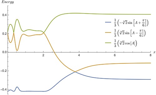
Figure 1. The partial adiabatic energies numbered 1, 2, 3 for the three state coupled oscillator. The horizontal axis x refers to linear distance and the vertical axis refers to the partial adiabatic energies. energies. The curve numbering in the plot corresponds to equation numbering of the model but plotted only the colour highlighted portion of the expressions. The curve numbered 1 arises from Equation (2) after subtracted from $\frac{X_1}{3}$ term and the curve numbered 2 arises from Equation (3) after the subtraction from $\frac{X_1}{3}$ term and so on and so forth. The dashed curve numbered 4 from Equation (5) is unique in the sense that it is not state dependent and common to all three adiabatic states. If there is a cusp in this curve, this is a strong indication that the system possesses a triple point. All other expressions which involve Equation (5) will also display similar cusp at the same location as can be seen in Figure 1. A close-up look reveals that all curves are approximated as straight lines near 0.4 and intersect exactly at 0.4.

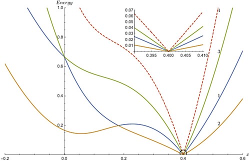
In Figure 1, there are four curves as a function of distance, x, representing harmonic stretching from the one-dimensional coupled oscillator problem, three of which represent partial adiabatic energies corresponding to three states which are obtained after the evaluation of the highlighted portion of the analytical expression seen in Equations (2)–(4) or in Equations (13)–(15) (evaluated portion highlighted in different colours) and all of them show a cusp at 0.4 suggesting it is a triple point location. The labelling of the curves suggests that they correspond to the numbered equation from which corresponding curves are produced. (The name ‘partial adiabatic energy’ makes sense as the contribution from the average of diabatic energies at a given point is subtracted out from the complete state-specific expression and therefore whatever the rest evaluates will not be equal to the state-specific total adiabatic energy.) The reason for the presence of cusp comes from Equation (5) which contributes equally to the evaluation of partial energies since it remains invariant irrespective of state in which it occurs and hence, is unique and characteristic of a typical molecular system with triple degeneracy. The last curve (dashed) is from Equation (5) alone denoted as $Y^{1/6}$ showing the similar behaviour and hence it is easy to conclude that the cusp in the partial energies is due to the existence of similar cusp found in the contributing expression seen in Equation (5) to the overall model set. A close look at the vicinity of the cusp clearly shows the perfect linearity for the partial energy curves as well as the state-independent unique curve for a typical system (see the top inset plot in Figure 1). In addition, all four cusps coincide well into one another exactly at same point.

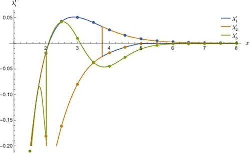
The cause of cusp in a triply degenerate molecular system is explained and now in a slightly different situation, when there are multiple doubly degenerate points isolated from one another instead of a single triple point, the cause of independent cusps arises from the angular part of the model but not from the unique common factor, $Y^{1/6}$ as explained above. However, the angular part whose analytical form (see the legends in Figure 2) varies from state to state, i.e. state-dependent quantity unlike the state-independent common factor. In Figure 2, the angular portion alone is shown revealing the presence of cusp clearly and hence, it is easy to conclude that the angular part is the reason for the cusp seen 1D cut of model PES of ${\mathrm{O}}_2{\mathrm{H}}^{+}$.

Figure 2. In the PES of ${\mathrm{O}}_2{\mathrm{H}}^{+}$, it is found that there is no triple degeneracy in the lowest three electronic states but only doubly degeneracies interconnecting the three surfaces (states). In this plot, the existence of doubly degenerate point is proven to have arisen from the angular factor involving pre-defined quantity which is defined in Equation (12(12) $\begin{array}{rl}& A=\frac{1}{3}\arg (X_3+\sqrt{X_5})\end{array}$(12) ). The magnitude of angular factor differs state wise as a function of x due to the opposing sign of the phase factor and also the differences in the form of the function itself. The $x\mathrm{axis}$ refers to linear distance and the curve from angular factor varies as x varies and hence invoking π in x axis is not appropriate.

How the common factor $Y^{1/6}$ or Equation (5) produces a cusp when there is a triple point in PES (numerically how this happens). For this, one must look at the individual terms the factor is composed of. There are three such terms, $X{3}^2$, $27X5$, $X_3\sqrt{108X_5}\cos (\frac{1}{2}\arg (X_5))$ in the summation of Equation (5) and in Figure 3, each one of them are plotted as a function of x separately, with the form of the term being shown next to the curve it belongs to. The dashed curve is same as the one in Figure 1 and is the grand total of just mentioned three terms to the power raised to 1/6. Even though individual terms do not show cusps the grand total does (dashed curve). It is easy to see that near the vicinity of the cusp, all three terms (their respective curves) pass through 0 with one of them being absolutely 0 everywhere i.e. the yellow curve corresponding to the term $X_3\sqrt{108X_5}\cos (\frac{1}{2}\arg (X_5))$ for reasons not so explicit to us. The summed up curve, however, numerically survives appreciably due to the evaluation of higher order root of summed up values which is almost close to zero limit and higher order root ultimately magnifies the resulting values. In the close up view, flat region and the spiked cusp where the derivative is ill-defined can be seen clearly. Table 1 is divided into two parts with a divider and in the top portion of the divider, few values near the flat region are listed for the individual terms to show their order of magnitude. The middle column (term) vanishes everywhere including the range outside of the specified one here and therefore, can be omitted in calculating $Y^{1/6}$. The second and fourth columns do not follow exactly the flatness but rather shallow even though their magnitudes are close to zero in the specified range. The last column values are higher because of higher order root of summed up values which are rather always small in this range. Therefore, this column of numbers clearly indicates that for the chemical systems (not necessarily a physical one such as coupled oscillator dealt with here) with triple point, the term $Y^{1/6}$ alone is mainly responsible for the cusp because of the presence of higher order root as part of its expression. The bottom portion of the divider in Table 1 is for the chemically realistic molecule ${\mathrm{O}}_2{\mathrm{H}}^{+}$ which does not show a triple point anywhere in its PES but only few doubly degenerate points connecting any two states at a time. Because of the independent existence of double degeneracies in the exemplified system it is clear that $Y^{1/6}$ factor does not show any cusp as obvious from its numerical values (kept on decreasing as x increases and this trend is not the same as the one observed in the top portion of Table 1) in the last column. Hence, it is concluded that the origin of cusp arises from the angular part of the full expression as exemplified in Figure 2 but not from the $Y^{1/6}$.

Figure 3. Equation (5) is plotted term wise separately and as a total sum of the expression. Each term in Equation (5) does not have any specific meaning when stand alone and arises as a result of mathematical simplification. It is possible to see that the middle term in Equation (5) does not contribute to the sum. The horizontal line is for this term. It is claimed that the cusp arises because of the presence of higher order root within which values close to zero limit occurs. Upon evaluation, this leads to values of appreciable magnitude (see Table 1).

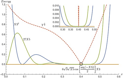
Table 1. Variation of terms present in $Y^{1/6}$ in Equation (5) as a function of x within a specific range. The last column refers to the blown up magnitudes after the sixth root of sum of three terms. The middle column remains at zero as x varies (visible in Figure 3 as a yellow straight line at zero in y-axis) and hence, the first and third columns only contribute to the sum and its higher order root. The first block of values are from the adiabatic coupled oscillator while the second block refers to the values from the one-dimensional cut from the potential energy surface of triatomic ${\mathrm{O}}_2{\mathrm{H}}^{+}$ ion. The dense grid is not required to highlight the points we want to emphasise upon and hence kept sparse. The factor $Y^{1/6}$ produces cusp in the oscillator model while it does not produce any cusp in the realistic triatomic model. Here, the appearance of cusp is not due to $Y^{1/6}$ but due to the angular factor present in the complete model expression given in Equations (2)–(4) or Equations (13)–(15) and the angular part is shown as legends in Figure 2. If any real molecule has triple degeneracy, then surely $Y^{1/6}$ will be the factor producing the cusp similar to the case of oscillator. In the chosen example of triatomic case, this situation does not arise.

		$6\sqrt{3}\sqrt{X_5}$
x	$X_3^2$	$\cos [\frac{\arg [-X_5]}{2}]X_3$	$27X_5$	$Y^{1/6}$
0.35	$2.33999\times {10}^{-5}$	0	$5.36564\times {10}^{-4}$	0.287096
0.36	$4.39959\times {10}^{-6}$	0	$1.68456\times {10}^{-4}$	0.236019
0.37	$4.91911\times {10}^{-7}$	0	$3.5625\times {10}^{-5}$	0.18181
0.38	$2.13668\times {10}^{-8}$	0	$3.68978\times {10}^{-6}$	0.124428
0.39	$9.26327\times {10}^{-11}$	0	$6.75744\times {10}^{-8}$	0.0638356
0.4	$6.74161\times {10}^{-95}$	0	$7.1103\times {10}^{-94}$	$3.03299\times {10}^{-16}$
0.41	$1.13148\times {10}^{-10}$	0	$9.12296\times {10}^{-8}$	0.0671087
0.42	$3.18886\times {10}^{-8}$	0	$6.73129\times {10}^{-6}$	0.137518
0.43	$8.97569\times {10}^{-7}$	0	$8.79809\times {10}^{-5}$	0.211251
0.44	$9.82396\times {10}^{-6}$	0	$5.64795\times {10}^{-4}$	0.288332
0.45	$6.40225\times {10}^{-5}$	0	$2.45136\times {10}^{-3}$	0.36878
0	0.00157103	0	$9.39096\times {10}^{-8}$	0.340959
1	0.00196392	0	0.0000698633	0.355946
2	0.00131599	0	$1.06237\times {10}^{-6}$	0.33108
3	0.000257936	0	0.00028667	0.285768
4	0.000183098	0	$4.59522\times {10}^{-6}$	0.239281
5	0.0000492599	0	0.0000212095	0.203236
6	0.0000338354	0	0.0000226246	0.194206
7	0.0000303615	0	0.0000232899	0.195865
8	0.0000290261	0	0.0000235575	0.193557

4. Derivative computation of the model

Coming to the derivative calculation of the coupled adiabatic curves/surfaces in general, getting an exact analytical expression for the first-order derivative is complicated and a herculean task even for the system as simple as an one-dimensional oscillator and therefore, one need to resort to the numerical approximation which is relatively easy and fast. Here, derivatives computed and shown are obtained via numerical methods. It is true that derivative is ill defined at degeneracy and no longer computable. However, this problem happens exactly at this point and not elsewhere and even at infinitesimal neighbourhood the derivative is found to be smooth. There is no analytical linear relationship transforming diabatic derivatives to adiabatic ones to circumvent this problem of singularity at degeneracy. Exact derivative (first order) expression in the adiabatic representation is possible in principle without resorting to numerical approximation as is reported in this work. Automatic differentiation is possible if a closed-form expression meant for the first-order derivatives is made possible if the diabatic representation is pure analytic and the success of separation of real and imaginary parts of the obtained result. In Figure 4, first-order derivative of diabatic and adiabatic curves is shown for three states and this figure is also described in the form of Table 2 showing some of the features not obvious from Figure 4. The discrete points are the continuous linear derivatives computed from the quadratic diabatic curves and can be either increasing or decreasing order. These points are listed under the headings, $V_{11}^{\mathrm{\prime }}$, $V_{22}^{\mathrm{\prime }}$ and $V_{33}^{\mathrm{\prime }}$ with uniform colour code in Table 2. The solid line refers to the derivatives from the adiabatic model curve which does not merge with those from the diabatic function everywhere because of the presence of cusps which plays the role of sign reversal on either side of the cusp resulting in discontinuities in the derivative line as can be seen from the encircled ellipse in which the actual jumping takes place. This is magnified in the inset plots displaying the jumping and sign reversal from positive to negative or vice versa (resembling a mutual crossing line). At the triply degenerate point, the derivative is not computable predicting infinity. However, this is not visible in graphical plot as this is an infinitely single point divergence and in the neighbourhood, it is converged to a finite value. In the table, it is explicitly written as infinity. The reason for the use of colour coding in the table is to find out approximately the location of discontinuities in derivatives. As is clearly seen, the diabatic derivatives are uniformly highlighted with the same colour but in the adiabatic derivatives, the highlighting colours differ along the columns. For example, in the third column with the heading, ${\lambda }_1^{\mathrm{\prime }}$, adiabatic derivatives are the same as the diabatic ones for the first few rows with the same coding and after this, colour coding for the adiabatic case differs as it merges with the derivatives from the diabatic column under the heading, $V_{33}^{\mathrm{\prime }}$ for few more rows. Then again for few rows, highlighting colour changes as the derivatives from the adiabatic case merge with the diabatic column under the heading, $V_{22}^{\mathrm{\prime }}$. In total there are two places derivative changes its sign with the sudden jump for the lowest adiabatic state which can also be verifiable by looking at Figure 4. Similarly, there is one discontinuity each in the higher level adiabatic states as per the colour coding shown for them.

Figure 4. The first derivatives of ${\lambda }_i$ denoted as ${\lambda }_i^{\mathrm{\prime }},i=1,2,3$, of coupled adiabatic curves are shown along with the discrete derivative points from the corresponding diabatic curves. To show abrupt jump as clear as possible both in sign reversal and magnitude, it is better to use continuous line for the adiabatic derivative case and this is not so in the case of diabatic derivatives and hence, a dot representation is preferred. The diabatic derivative points follow linear pattern with the points being at same colour while this is not so for the adiabatic case. In this case, derivative becomes discontinuous at a point where derivative is ill defined (or numerically unstable) and till it reaches such a point it is smooth and continuous. The discontinuity can happen either at a triply degenerate point or at a doubly degenerate point and results in merging of derivatives from one diabatic state to another. In the inset plots, how switching of adiabatic derivatives takes place is shown at a close up view. If the line and points are of different colour, then it is an indication that switching of adiabatic derivatives took place. Looking at this figure together with Table 2 will make the things clear.

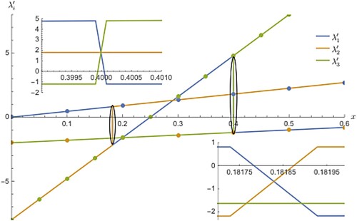
Table 2. Here, Figure 4 is represented in a table format for more clarity. The colour specification is not used to distinguish among the symbols but to know where the discontinuity in derivative happens by way of sudden change in colour code. This can be seen in alternate columns, one with no change in colour code and the next one with sudden change of colours. At the top of second, fourth and sixth columns, $V_{11}^{\mathrm{\prime }}$ denotes first derivative of diabatic potential, $V_{11}$, $V_{22}^{\mathrm{\prime }}$ denote first derivative of diabatic potential, $V_{22}$, $V_{33}^{\mathrm{\prime }}$ denote first derivative of diabatic potential, $V_{33}$ and in the third, fifth and seventh columns, ${\lambda }_1^{\mathrm{\prime }}$ denotes first derivative of adiabatic potential, ${\lambda }_1$, ${\lambda }_2^{\mathrm{\prime }}$ denote first derivative of adiabatic potential, ${\lambda }_2$, ${\lambda }_3^{\mathrm{\prime }}$ denote first derivative of adiabatic potential, ${\lambda }_3$. The colouring of columns is essential and is shown for proper understanding. As expected, the derivative is continuous in the case of diabatic state while it is not so for the adiabatic state. The discontinuity happens because of the presence of cusp or conical intersection on either side of which the derivative is continuous but of opposite sign. This sign reversal is the cause for the discontinuity. At cusp (an unique point), it cannot be computed. From the colour changes along an adiabatic column, it is possible to tell how many cusps are there in a given state. The colour is uniformly coded for the diabatic case. The triple point is obvious from the infinite derivative.

For the sake of clarity, the coupled oscillator is an useful example to explain the characteristics of the proposed model in a way any one can get it nicely. But, when we come to the second example of PES of ${\mathrm{O}}_2{\mathrm{H}}^{+}$ ion the clarity is bit reduced as 1D cut of derivative PES are closely spaced and the crossing of diabatic curves falls in between the closely spaced curves, thus, the cusp and its derivative changing the direction rapidly. In Figure 5, the adiabatic and diabatic derivative curves as a function of x (here x denotes bond length in a real molecule and not to be confused with the same x given in the context of oscillator problem). The reader can also use some other variable name (example being r) instead of x as it is already in use in the previous example. However, this will not pose any problem since they are two different problems, are shown with both the types merging one over the other in the long range in the zero limit, a typical behaviour seen in any usual potential curves. There are two derivative crossing at two distinct places, one near 4 bohr and another near 2 bohr. As there is no magnification switching (jumping) of adiabatic derivatives between the states and the merging with diabatic derivatives is hard to identify in this case but surely there is a switching existing like the one in Figure 4. When solid line and the points over it differ in colour then it is an indication that the derivative undergoes the change of state by merging with the discrete derivatives from the diabatic curves. The diabatic derivatives do not undergo sudden jumping as the individual curves are perfectly decoupled and therefore, smooth everywhere even though it assumes both positive and negative magnitudes. The increment used has been deliberate chosen as the objective is to prove the feasibility of integration of functions with cusps in multi-state fitting calculations.

5. Integration of the model expression

Now, turning to the integral properties of triple-valued analytical PESs mutually interconnected via the set of multiple seams it is found that the presence of several sharp cusps (CIs) in the smooth model surface does not affect the outcome of the integration and its square integrability and always it turns out to be finite inside a finite interval and never diverge. At the cusp which can be a triply or doubly degenerate point, the integral effectively vanish unlike computing a derivative at this point which is ill defined and not computable and therefore do not contribute to the net sum when integrating over a finite region containing one or more cusps. The integral evaluates to non-zero finite values away from the cusps. The integration of potential energy function finds application in the molecular theory of real gases to get a closed formula for second-order virial coefficient describing the deviation from the ideal behaviour. Hence, the integration is very much needed to calculate the second-order coefficient to understand the transition from ideal to real behaviour of gases. In this work, we apply the integration to both the model examples taken up for illustration. In Table 3, we present the square integrable values of the coupled oscillator curves with an increment of 0.1 up to the maximum limit of 0.6 for three states together. Initially, it is zero and then as the distance increases the integrated values increase but the main message is they are computable and smooth and not facing numerical difficulties due to the presence of cusps. Similarly, in the same table the values from the one-dimensional coupled cuts of ${\mathrm{O}}_2{\mathrm{H}}^{+}$ PES are tabulated with an constant increment of 1 with the range varying between 0 and the maximum of 8. Therefore, this table clearly shows the integrability or square integrability of the chosen analytical model function and can be applied to situations which demands the use of calculations of numerical integration similar to the one when dealing with the real behaviour of gases.

Figure 5. This is similar to Figure 4 but for a realistic molecule ${\mathrm{O}}_2{\mathrm{H}}^{+}$ ion. The derivatives apply to the lowest three electronic states of ${}^3{A}^{\mathrm{\prime \prime }}$ symmetry. The discrete points are from diabatic curves while the solid line refers to the adiabatic curves. No Table similar to Table 2 is given for this molecular system as it has no triple point in PES. In the absence of triply degenerate point, the presence of isolated doubly degenerate point linking two states produces discontinuities in the derivatives at two places, one near at 4 bohr and other at 2 bohr. This discontinuity in adiabatic derivatives causes them to merge with those from diabatic curves. This is clear from the dissimilarities in colours between the points and the solid line.

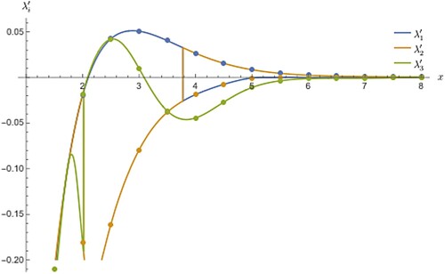
Table 3. The integral values of two models considered in this work. The presence of CIs along the curves does not pose any problems to the evaluation of integrals over a finite interval with the lower limit being fixed at zero and the upper limit varying as a function of integral sum. The wider instead of finer discreteness is justified as the point to be established is to prove the feasibility of integration of functions involved in conical intersections.

Coupled oscillator				Coupled curves of ${\mathrm{O}}_2{\mathrm{H}}^{+}$
x	${\displaystyle {\int }_0{\lambda }_1^2(x)}$	${\displaystyle {\int }_0{\lambda }_2^2(x)}$	${\displaystyle {\int }_0{\lambda }_3^2(x)}$	x	${\displaystyle {\int }_0{\lambda }_1^2(x)}$	${\displaystyle {\int }_0{\lambda }_2^2(x)}$	${\displaystyle {\int }_0{\lambda }_3^2(x)}$
0	0	0	0	0	0	0	0
0.1	0.000010125	0.046112	0.081902	1	0.241167	0.52943	0.634028
0.2	0.00026062	0.0500474	0.134464	2	0.294571	0.53699	0.644466
0.3	0.00029262	0.0521838	0.166386	3	0.375924	0.555264	0.645135
0.4	0.00416462	0.0600914	0.184448	4	0.43468	0.602564	0.645611
0.5	0.0134666	0.081364	0.23056	5	0.492359	0.648149	0.648789
0.6	0.0176686	0.128455	0.449472	6	0.551265	0.68975	0.689754
				7	0.61018	0.730203	0.658718
				8	0.669095	0.770233	0.663919

6. Conclusion

A simultaneous analytical model is presented in a form which could be easily used/adapted to any combined fitting of ab-initio data points from three electronic states. The result is a direct consequence of analytical diagonalisation of a typical $3\times 3$ generalised diabatic matrix. The essential feature of the model is that it is capable of predicting seam trajectory running through all three electronic surfaces, something not found in the literature. Additionally, few properties of the model are also discussed. It is explained how the model function is able to account for the presence of sharp cusp (that is about the presence of feature responsible for such cusp). While taking derivative, the model allows to compute everywhere in PES smoothly except at the point of degeneracy where it is not computable. The interpretation is that this simultaneous model can be used in harmonic analysis since it is possible to calculate first and second derivatives both numerically (practically viable) as well as analytically (in principle). However, the integration of surface can be done easily even at the point of degeneracy. It proves that it is finite everywhere within the molecular PES and therefore can be used in computing viral coefficients encountered in the molecular theory of gases.

Acknowledgments

It is gratefully acknowledged the support of the University and Department of Chemistry for necessary resources.

Disclosure statement

No potential conflict of interest was reported by the author(s).

References

- J. Katriel and E. Davidson, Chem. Phys. Lett. 76 (2), 259–262 (1980). doi:10.1016/0009-2614(80)87016-3
- S. Matsika and D.R. Yarkony, J. Am. Chem. Soc. 125 (35), 10672–10676 (2003). doi:10.1021/ja036201v
- S. Matsikain Reviews in Computational Chemistry, Chap. 2, (2007), pp. 83–124.
- S. Matsika and D.R. Yarkony, J. Chem. Phys. 117 (15), 6907–6910 (2002). doi:10.1063/1.1513304
- S. Matsika and D.R. Yarkony, J. Am. Chem. Soc. 125 (41), 12428–12429 (2003). doi:10.1021/ja037925+
- L. Blancafort and M.A. Robb, J. Phys. Chem. A 108 (47), 10609–10614 (2004). doi:10.1021/jp045985b
- J.D. Coe and T.J. Martínez, J. Am. Chem. Soc. 127 (13), 4560–4561 (2005). doi:10.1021/ja043093j
- S. Matsika, J. Phys. Chem. A 109 (33), 7538–7545 (2005). doi:10.1021/jp0513622
- K.A. Kistler and S. Matsika, J. Chem. Phys. 128 (21), 215102 (2008). doi:10.1063/1.2932102
- S. Han and D.R. Yarkony, J. Chem. Phys. 119 (22), 11561–11569 (2003). doi:10.1063/1.1623483
- S. Han and D.R. Yarkony, J. Chem. Phys. 119 (10), 5058–5068 (2003). doi:10.1063/1.1591729
- S. Matsika, Chem. Phys. 349 (1–3), 356–362 (2008). doi:10.1016/j.chemphys.2008.02.027Electron Correlation and Molecular Dynamics for Excited States and Photochemistry.
- P. Krause and S. Matsika, J. Chem. Phys. 136 (3), 034110 (2012). doi:10.1063/1.3677273
- I.B. Bersuker, The Jahn Teller Effect and Vibronic Interactions in Modern Chemistry (1984).
- R. Englman, The Jahn Teller Effect in Molecules and Crystals (1972).
- I.B. Bersuker and V.Z. Polinger, Vibronic Interactions in Molecules and Crystals, Vol. 101 (1989).
- X.Y. Liu, G. Cui and W.H. Fang, Theor. Chem. Acc. 136 (1), 8 (2016). doi:10.1007/s00214-016-2029-z
- Y.S. Baek, S. Lee, M. Filatov and C.H. Choi, J. Phys. Chem. A 125 (9), 1994–2006 (2021). doi:10.1021/acs.jpca.0c11294
- H.J. Werner, P.J. Knowles, G. Knizia, F.R. Manby and M. Schütz, WIREs Comput. Mol. Sci. 2 (2), 242–253 (2012). doi:10.1002/wcms.v2.2
- H.J. Werner, P.J. Knowles, F.R. Manby, J.A. Black, K. Doll, A. Heßelmann, D. Kats, A. Köhn, T. Korona, D.A. Kreplin, Q. Ma, T.F. Miller, A. Mitrushchenkov, K.A. Peterson, I. Polyak, G. Rauhut and M. Sibaev, J. Chem. Phys. 152 (14), 144107 (2020). doi:10.1063/5.0005081
- H.J. Werner, P.J. Knowles, G. Knizia, F.R. Manby, M. Schütz, P. Celani, W. Györffy, D. Kats, T. Korona, R. Lindh, A. Mitrushenkov, G. Rauhut, K.R. Shamasundar, T.B. Adler, R.D. Amos, S.J. Bennie, A. Bernhardsson, A. Berning, D.L. Cooper, M.J.O. Deegan, A.J. Dobbyn, F. Eckert, E. Goll, C. Hampel, A. Hesselmann, G. Hetzer, T. Hrenar, G. Jansen, C. Köppl, S.J.R. Lee, Y. Liu, A.W. Lloyd, Q. Ma, R.A. Mata, A.J. May, S.J. McNicholas, W. Meyer, T.F. Miller III, M.E. Mura, A. Nicklass, D.P. O'Neill, P. Palmieri, D. Peng, K. Pflüger, R. Pitzer, M. Reiher, T. Shiozaki, H. Stoll, A.J. Stone, R. Tarroni, T. Thorsteinsson, M. Wang and M. Welborn, MOLPRO, version, a package of ab initio programs see.
- F.G.D. Xavier and A.J.C. Varandas, Mol. Phys. 119 (10), e1904157 (2021). doi:10.1080/00268976.2021.1904157
- A.J.C. Varandas, J. Chem. Phys. 107 (3), 867–878 (1997). doi:10.1063/1.474385
- A. Aguado, C. Suárez and M. Paniagua, J. Chem. Phys. 98 (1), 308–315 (1993). doi:10.1063/1.464676
- J. Murrell, S. Carter, I. Mills and M. Guest, Mol. Phys. 42 (3), 605–627 (1981). doi:10.1080/00268978100100491
- S. Nangia and D.G. Truhlar, J. Chem. Phys. 124 (12), 124309 (2006). doi:10.1063/1.2168447
- F.G.D. Xavier, Int. J. Quantum Chem. 123 (20), e27199 (2023). doi:10.1002/qua.v123.20
- F.G.D. Xavier, ChemPhysChem 24 (15), e202200909 (2023). doi:10.1002/cphc.v24.15
- Wolfram Research, Inc., Mathematica, Version 12.0 Champaign, IL, 2019.