The dipole moment of supercritical water – local vs. mean-field polarisation contributions

Abstract

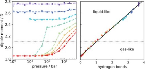
Supercritical water has attracted much attention from both fundamental and technological perspectives, based largely on its ability to solvate other molecules. Predicting and controlling this requires a deeper understanding of water's polarisation behaviour. Using the computationally efficient Self-Consistent Electrostatic Embedding method, we were able to calculate the water dipole moment over an unprecedented range of thermodynamic conditions, covering gas, liquid and supercritical states, with large simulation systems and a high-level quantum mechanical method. We find a discontinuous change in the dipole moment along subcritical isotherms, corresponding to the sharp transition between the vapour and liquid states, with the latter exhibiting induced dipole moments between 0.5 and 0.9 D, depending on the temperature. In contrast, the dipole moment changes continuously from gas-like to liquid-like behaviour in the supercritical regime, allowing the degree of polarisation to be controlled through manipulating temperature and pressure. The dipole moment was found to be linearly related to the average number of hydrogen-bonded neighbours of water, emphasising the key role of local interactions to the polarisation process. Mean-field approaches based on a dielectric continuum representation of the solvent are unable to predict this behaviour due to the neglect of local interactions.

GRAPHICAL ABSTRACT

Keywords:

• Dipole moment
• dielectric constant
• phase equilibrium
• molecular dynamics
• QM/MM

1. Introduction

Water is one of the most studied substances, not only because it is essential to life and biology but also because of the vital role it plays in many industrial processes [1,2]. In fact, liquid water exhibits an extensive range of ‘anomalous’ behaviour [3–6], with Pettersson et al. proclaiming it to be the most anomalous liquid [7]. Much of the practical importance of water can be attributed to the unique environment that liquid water provides to preferentially solvate other molecules. This can be used to facilitate the extraction of valuable compounds or to promote desired chemical reactions. The solvation environment can be tuned by adjusting the thermodynamic conditions; for example, liquid water typically demixes from non-polar solutes, but is able to solvate these same species when in the supercritical state [8,9].

In fact, supercritical water has demonstrated potential to act as a new green solvent to extract valuable products from biomass, break down unwanted compounds in wastewater and facilitate the gasification of biomass to generate hydrogen [10–17].

Understanding the underlying reasons for this dramatic change in solvation behaviour has been the subject of numerous scientific studies, yet many aspects, such as the structure and nature of hydrogen bonds within supercritical water, are still up for debate. At ambient conditions, water tends to form a continuous network of H-bonds, but the H-bond dynamics speeds up significantly under supercritical conditions [18], with some authors arguing that the molecular structure of water is more likely to exist as a series of continuously formed and destroyed clusters [19]. More recently, Schienbein and Marx [20] went as far as to state that supercritical water is not hydrogen-bonded at all. Specifically, they concluded that the H-bond lifetime in supercritical water was too short to explain the observed intermolecular vibrations, which instead could be well described by isotropic van der Waals interactions alone.

The molecular charge distribution, primarily characterised by the dipole moment, plays a significant role in the interaction of water molecules, which in turn controls its thermophysical properties (e.g. enthalpy of vaporisation, chemical potential, dielectric constant, etc.) [21–24]. When water is isolated from other molecules or in a dilute gas phase, its dipole moment is 1.855 D [25]. However, in the liquid phase, an electric field is generated by surrounding molecules, resulting in a distortion of the structure and electronic cloud of the molecule [26]. While this distortion is energetically unfavourable, the system receives a net decrease in the free energy resulting from the strongly enhanced intermolecular interactions between the polarised molecules. This process leads to a significant enhancement of the molecular dipole moment in the liquid phase [8,27–29]. However, it is notoriously difficult to quantitatively estimate the molecular dipole moment in condensed phases, due to the challenge of decoupling individual molecules and their electronic properties from the surrounding molecules [30]. In fact, the first reported ‘experimental measurement’ of the dipole moment in liquid water was actually determined through theoretical calculations based on ice Ih rather than by direct measurement in the liquid phase [31]. Later, Badyal et al. [32] estimated the degree of interatomic charge transfer from data obtained via neutron and X-ray diffraction techniques, and used that to calculate the dipole moment of liquid water. They reported a value of 2.9 D, representing an enhancement of $\sim 1$ D over the gas-phase value, but with a large uncertainty of $\pm 0.6\mathrm{D}$. Interestingly, this value agrees quite well with a subsequent estimate of 2.95 D by Gubskaya and Kusalik [33], which was obtained through a combination of experimental refractive index values, electronic response properties from ab initio techniques, and local fields and field gradients from classical simulation data.

Attempts to estimate the liquid water dipole moment from computer simulations have been much more frequent, although they are still fraught with challenges. Classical non-polarisable models based on fixed charges/dipoles are unable to respond to the polarising environment and are hence unsuitable for this purpose, and even polarisable models generally tend to underestimate the degree of polarisation in the liquid [30]. As such, previous efforts to calculate liquid phase dipole moments were primarily based on ab initio molecular dynamics (AIMD) or quantum mechanics/molecular mechanics (QM/MM) methods (see Ref. [30] for a review of such studies for water at ambient conditions). AIMD treat the entire system quantum mechanically and then partition the electron density into individual molecular contributions using methods such as maximally localised Wannier functions [34]. QM/MM methods, on the other hand, only treat the central molecule at the QM level, so no partition of the electron density is necessary, but approximate the remainder of the system at a less accurate classical level [35]. We have recently shown that the results of these two approaches can be reconciled, provided the effects of different QM/MM approximations are properly taken into account [30].

There have been prior attempts to quantify the dipole moment of water in the supercritical state, albeit much fewer than for ambient water [18,19,36–39]. All of those studies were carried out with AIMD and, due to the inherent computational expense of that method, most were limited to only a few state points using rather small simulation boxes. A notable exception is the recent state-of-the-art simulation study by Schienbein and Marx [39], which considered 20 state points, multiple simulation replicas per state point, and simulation boxes containing 128 water molecules each. While in the liquid or dilute vapour phase, the correlations between molecules are typically on the order of magnitude of their size, but as a system approaches its critical point, the correlation length will become larger and eventually diverge. In order to properly capture the physics of near-critical and supercritical systems, the size of the simulation must be significantly larger than the correlation length. This limits the systems that can be examined by computationally demanding methods like AIMD.

Recently we introduced a new QM/MM approach, termed Self-Consistent Electrostatic Embedding (SCEE), that provides accurate estimates of the molecular dipole moment in condensed phases with relatively low computational expense [30,40]. The benefit of this approach is that it allows phase space to be explored using highly efficient classical MD simulations, while computing electronic properties at high QM levels of theory – in fact, generally much higher than accessible to AIMD simulations. Previously, our group applied SCEE to determine the dipole moment of water under ambient conditions, obtaining a value of $\sim 2.8$ D that corresponds to an induced dipole of $\sim 0.95$ D with respect to the gas phase [30], in excellent agreement with previous AIMD calculations and experiment. SCEE has also proven to be accurate for other compounds besides water [40,41]; however, previous work was limited to the liquid phase.

In this work, we utilise a combination of MD and SCEE to examine the structure and polarisation of water across a broad range of conditions, including the liquid, vapour and supercritical regions. The paper is organised with the following structure. Section 2 describes the calculations performed in this work, first detailing the molecular dynamics simulations and then highlighting the key concepts behind the SCEE method and its application to the configurations captured by the MD simulations. In Section 3, we report the results of these calculations. In particular, we analyse the pair correlation functions and hydrogen bonding. At each of the simulated state points, we also examine the polarisation of the water molecules using the SCEE method, relating the statistics of the dipole moments to the fluid structure. Finally, Section 4 summarises the main findings of this work and directions for future investigations.

2. Methodology

2.1. Molecular dynamics simulations

To explore phase space and harvest molecular configurations for use in the SCEE method, we have carried out molecular dynamics (MD) simulations using GROMACS 2023 [42,43] on a periodic cubic box that contained 900 water molecules, corresponding to about 3 nm in length for the highest density systems. We used the Verlet leap-frog algorithm [44] to integrate the equations of motion with a time step of 2 fs. The simulations were performed within the NpT ensemble with the temperature controlled by the V-rescale thermostat [45] with a 0.1 ps time constant, and pressure controlled by a Parrinello-Rahman barostat [46] with time constant of 2.0 ps and compressibility of $4.5\times {10}^{-5}{\mathrm{m}}^3/\mathrm{bar}$.

We chose the TIP4P/2005 model [47] for the MD simulations, as it is considered to be one of the best performing non-polarisable water models available [48] and is able to describe the phase diagram of water with a good degree of accuracy over a wide range of conditions [49]. It is important to note that we have previously compared the results of SCEE calculations based on several models, including a polarisable one, and found the resulting dipole moment distributions to be independent of this choice, provided the model was able to realistically describe the structure of the liquid phase [30]; in particular, TIP3P was the only outlier in the above comparison, due to its well-known shortcomings in reproducing structural and thermodynamic properties of water. The water molecule was held rigid during the MD simulations by applying the LINCS constraint algorithm [50]. The Lennard-Jones potential had a cut-off of 1.2 nm applied, with long-ranged dispersion corrections added to both energy and pressure, while the particle-mesh Ewald method [51] was used to account for the long-range electrostatic interactions with a real-space cut-off of 1.2 nm.

MD simulations were run at state points spanning the vapour, gas, liquid and supercritical regions of the phase diagram, as depicted in Figure 1. Specifically, we considered the following temperatures (298, 400, 500, 600, 700, 800, 900 and 1000 K) and pressures (1, 2, 5, 10, 20, 50, 100, 200, 500, 1000, 2000 and 5000 bar). Figure 1 also shows the experimental vapour-liquid equilibrium line [52], as well as the one predicted by TIP4P/2005 [49]. Each MD simulation started from a pre-equilibrated water box at 298 K and 1 bar and was run for 5 ns, with 200 configurations being harvested from the last 4 ns of the run; successive configurations were spaced 20 ps apart to ensure they were sufficiently uncorrelated while maintaining sampling efficiency [53].

Figure 1. Pressure-temperature diagram for water. The solid line represents the experimental vapour pressure curve [52], and the dashed line represents the vapour pressure curve for the TIP4P/2005 model [49]. The symbols denote state points where simulations were performed in this work. Circles represent liquid states, triangles gas/vapour states, and stars supercritical states.

For the systems with higher density (i.e. corresponding to the lower temperatures; see below), we ran up to 6 additional replicas to improve the precision of the dipole moment estimates – see Table S1 for a full list of all state points run. Because the simulations started from the liquid state, we observed hysteresis at a temperature of 500 K when the pressure was lower than the model's vapour pressure (i.e. at 1, 2 and 5 bar). In those cases, we ran additional simulations starting from a pre-equilibrated vapour box (specifically, the outcome of the run at 600 K and 1.0 bar) using the same set-up as above except for the barostat settings; we controlled the pressure with the Berendsen barostat to achieve faster convergence and an isothermal compressibility of $0.1{\mathrm{m}}^3/\mathrm{bar}$, more representative of the gas phase.

Besides extracting configurations for SCEE, we also analysed the output of the MD simulations themselves. This analysis was performed using a range of tools available within GROMACS 2023 [42,43], for the trajectories obtained at each state point. Specifically, we computed the average density using gmx energy and compared it against the experimental density for each state point extracted from the NIST database [52]. To investigate the relationship between the dipole moment and the structure of water at different thermodynamic conditions, radial distribution functions (RDFs) were calculated for O-O, O-H, and H-H pairs using gmx rdf, making sure to eliminate intramolecular peaks. We also carried out an analysis of hydrogen bonds using gmx hbond. We consider two molecules to be hydrogen bonded if their hydrogen-acceptor distance was shorter than 0.35 nm and the hydrogen-donor-acceptor angle was lower than ${30}^{\circ }$. From the time-averaged total number of H-bonds $〈N_{\mathrm{Hbonds}}〉$ in the system, we calculate $〈N_{\mathrm{neig}}〉$, the average number of hydrogen bonded neighbours per water molecule, as (1) $〈N_{\mathrm{neig}}〉=2\left(\frac{〈N_{\mathrm{Hbonds}}〉}{N_{\mathrm{mols}}}\right)$(1) where $N_{\mathrm{mols}}$ is the total number of molecules in the system. The factor of 2 is applied to prevent double-counting.

2.2. Self-consistent electrostatic embedding

SCEE approaches the prediction of the dipole moment by ensuring a balance between computational efficiency and accuracy, and has been previously applied to calculate dipole moments for liquid water [30], aliphatic alcohols [40] and ketones [41]. A detailed description of the method has been presented in our previous publications [30,40], and here we limit ourselves to a brief overview. From each molecular configuration extracted from the MD runs described in Section 2.1, a spherical cluster of radius 2.0 nm is created and then converted to a format suitable for Gaussian 09 [54] using an in-house code [40]. Only the central molecule is treated at the QM level, while the MM level describes the surrounding cluster of molecules. This layering is achieved using the ONIOM formalism [55,56] on Gaussian 09, where the MM Lennard-Jones interaction parameters correspond to those of TIP4P/2005. For each configuration, three QM/MM calculations are carried out, each with a different value for the dipole moment (and hence point charges) of the surrounding MM molecules. The QM calculations made use of the B3LYP functional [57,58] and the aug-cc-pVTZ basis set [59], which have been shown to yield very accurate dipole moment values [30,60,61]. This level of theory was applied both in the geometry optimisation step with ONIOM and in the subsequent electrostatic embedding single-point calculation to obtain the QM dipole moment [40,41]. An analytical correlation was then established between the resulting QM dipole moment (${\mu }_{\mathrm{QM}}$) and the pre-set dipole moment of the surrounding MM molecules (${\mu }_{\mathrm{MM}}$), thus allowing us to obtain the self-consistent dipole moment for that configuration (i.e. where ${\mu }_{\mathrm{QM}}={\mu }_{\mathrm{MM}}$). These dipole moments were then averaged over all configurations for each state point, yielding a full distribution of dipole moments at a given set of conditions. A final note should be made; in several gas-phase configurations there were no neighbouring molecules within a radius of 2.0 nm from the central molecule, in which case the QM/MM calculation becomes identical to a single-molecule optimisation in vacuum. Rather than repeat a series of identical calculations, we simply assigned a value of 1.856 D to those particular configurations, since that was the previously determined dipole moment of an isolated molecule at the B3LYP/aug-cc-pVTZ level of theory [30].

For comparison, we also calculated the water dipole moment at different conditions using the IEFPCM model [62] as implemented in Gaussian 09. These calculations consider only a single water molecule at the QM level, surrounded by a uniform dielectric continuum. For all these calculations, we selected ‘water’ as the solvent but changed the value of the dielectric constant to describe the changes in solvent conditions with temperature and pressure. We obtained values for the dielectric constant at the different state points from the correlation provided by Fernandez et al. [63].

3. Results and discussion

3.1. Density

Although not the main objective of this paper, comparing the density obtained in MD simulations to experimental data allows us to (re)validate the performance of the TIP4P/2005 model over a wide range of temperatures and pressures. Such a comparison in shown in Figure 2, where the experimental data were taken from the NIST database [52]. There is excellent agreement between simulation and experiment across the whole phase diagram, the only exception being a few points close to the vapour-liquid coexistence pressures at 400, 500 and 600 K. This is due to the well known slight underestimation of the experimental vapour pressure by TIP4P/2005 [49] (see also Figure 1). For this reason, those points were not considered in the subsequent analysis. The agreement observed in Figure 2 gives us confidence that TIP4P/2005 does indeed provide an accurate description of water at supercritical conditions, and hence the configurations extracted from our MD simulations can be used to estimate the corresponding dipole moments.

Figure 2. Variation of the density of water with pressure along different isotherms. The solid lines represent experimental data taken from the NIST Chemistry WebBook [52]. The filled circles are for the TIP4P/2005 model [49] from the MD simulations performed in this work.

3.2. Dipole moment

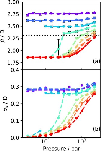
In Figure 3(a), we show the average dipole moments calculated using SCEE as a function of pressure along different isotherms; the error bars represent the uncertainty of each calculation. Below the critical temperature (i.e. isotherms for 298, 400, 500 and 600 K), the dipole moment shows a discontinuous change, going from values close to 1.856 D below the vapour pressure, corresponding to the gas-phase dipole moment, to values between 2.3 and 2.8 D in the liquid state. In the liquid regime, the mean dipole moment is mostly insensitive to changes in pressure, being practically constant along each isotherm, at least until very high pressures are reached. Above $\sim 1000$ bar, however, there is a slight but noticeable increasing trend in the dipole moment, which roughly corresponds to the region where the density of the liquid begins to show a significant increase (Figure 2). Temperature seems to have a much more significant influence, with the average dipole moment decreasing as the temperature increases at constant pressure. We note also that the average dipole moments at 298 K and $P<1000$ bar agree well with our previous estimate of $2.76\pm 0.03$ D for liquid water at room temperature [40]. In contrast, in the supercritical regime, the dipole moment increases continuously from values typical of the gas phase (i.e. around 1.85 to 2.0 D) to values characteristic of the liquid state (i.e. close to 2.4 D). Our SCEE results are in good agreement with previous AIMD simulations of supercritical water, which also observed a general decrease of the dipole moment with temperature and an increase with pressure (or, equivalently, density) [18,19,36–39]. However, by considering many more state points and much larger simulation boxes, we are able to follow the changes in the degree of polarisation of water with temperature and pressure in much greater detail.

Figure 3. The variation of the (a) mean and (b) standard deviation of the dipole moment with pressure along different isotherms. The points are colour-coded by temperature as in Figure 2. The error bars represent the 95% confidence intervals, and the dashed lines are to guide the eye. The dotted line in panel (a) shows the (fixed) value of the TIP4P/2005 dipole moment.

In Figure 4, we show a selection of dipole moment distributions obtained from the SCEE calculations to demonstrate the different behaviour below and above the critical temperature. Dipole moment distributions for the remaining state points are provided in Supporting Information. At 298 K (Figure 4(a)), all simulations for the selected pressure range correspond to the liquid state, so the dipole moment distributions practically overlap with each other, indicating the near lack of influence of the pressure in this regime, as discussed above. At 500 K, however, the system transitions from vapour to liquid, and the dipole distributions (Figure 4(b)) show an abrupt change – in the vapour phase, they are characterised by a very sharp peak around 1.856 D, while in the liquid phase they peak around 2.5 D but are much more spread out, ranging from just under 2.0 D all the way up to 3.5 D. Interestingly, there is practically no overlap between the vapour and liquid dipole distributions, with the latter starting immediately after the tail end of the former. The same trend is observed at 600 K (see SI).

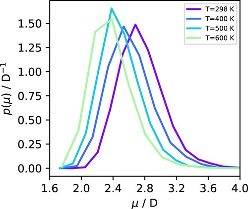
To obtain better statistics for the effect of temperature on the dipole moment distributions in the liquid phase, we take advantage of the negligible pressure dependence of the dipole moment below 1000 bar (see Figure 3) and average together all the data at each subcritical temperature for all pressures between the vapour-liquid transition point and 1000 bar (e.g. for 500 K, we averaged over 7 state points, from 10 to 1000 bar, inclusive). The resulting distributions are shown in Figure 5, where there is a clear gradual shift in the distribution to lower values as T increases, but the width of the distribution remains practically unchanged.

Figure 4. Dipole moment distributions for water at varying pressures and (a) 298 K. (b) 500 K and (c) 700 K.

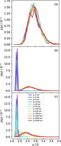
Figure 5. Dipole moment distribution in the liquid phase at different temperatures, averaged over pressures between the vapour-liquid transition and 1000 bar.

The distributions at 700 K (Figure 4(c)), representative of the approach to the supercritical state, show a markedly different behaviour. At very low pressures, where the system can be characterised as a gas, the distributions are practically identical to those for the vapour phase (i.e. a sharp peak around 1.856 D). As the pressure increases, however, the distributions start to develop a tail at the high end (see the line for 50 bar), which increases and eventually develops into a separate peak as the critical pressure is reached (see the line for 200 bar). Beyond this point, the peak continues to shift gradually to higher values and increases in width, becoming more similar to liquid-like dipole moment distributions. Notice, however, that even at the highest pressures along this isotherm, the system still exhibits a small number of gas-like configurations (i.e. the low-end tail of the distribution extends to values around 1.856 D). This behaviour is in marked contrast to that observed below the critical point, where there was a clear gap between vapour and liquid distributions (cf. Figure 4(b)).

To depict the changes in dipole moment distributions over temperature and pressure, we plot the standard deviation of those distributions for all state points in Figure 3(b). Although the data are noisy, it is interesting that the liquid phase dipole moment distributions all have roughly the same width, even though the average dipole moments decrease with temperature (cf. Figure 3(a)). This suggests that increasing temperature causes a shift in the entire dipole moment distribution to lower values, but does not significantly affect the degree of fluctuations, at least for the conditions examined here. The results for the gas/vapour state points are trivial, with the very low standard deviation reflecting the very sharp peaks of those distributions. This indicates, as expected, that dipole moment fluctuations are essentially absent, since molecules are practically isolated from each other with only occasional contacts. Finally, the supercritical regime shows a gradual increase in the width of the distributions, from gas-like to liquid-like behaviour, consistent with the above discussion and the data in Figure 4(c). Here, both temperature and pressure have a pronounced effect on both the average dipole moment and its fluctuations: both increasing with P and decreasing with T.

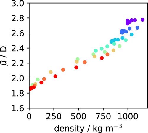
Comparing Figures 2 and 3(a), there is a clear similarity between the T and P dependence of the density and of the dipole moment of water. This relationship has been previously investigated by Sakuma et al. [64] and Kang et al. [38]. To quantify that more clearly, the dipole moment is plotted against the density in Figure 6 for all state points examined here. Although it is clear that the dipole moment generally increases with density, the correlation is far from perfect, particularly for the more dense states. In fact, at those conditions, the pressure seems to have a much stronger effect on the density than on the dipole moment, which leads to points with the same colour (i.e. along a given isotherm) to align as nearly horizontal ‘bands’ in the figure. The key message from this plot is that the changes in dipole moment of water are not simply caused by changes in density. To explain the dipole variations, we need to further investigate the detailed structure of water.

Figure 6. Variation of the average dipole moment with system density along different isotherms. The points are colour-coded by temperature as in Figure 2.

3.3. Water structure and hydrogen bonding

We begin by analysing radial distribution function (RDF) data for OO, OH and HH interactions at each state point. As in Figure 4, we focus on the data for 298 K, 500 K and 700 K and varying pressure as representative examples of the different regimes – see Figures 7, 8 and 9. RDFs for the remaining state points are provided in SI.

Figure 7. RDFs obtained at 298 K with varying pressures for (a) OO. (b) OH and (c) HH.

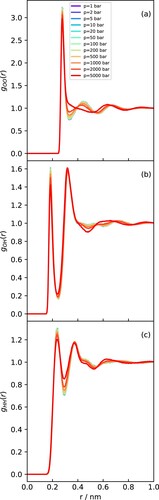
Figure 8. RDFs obtained at 500 K with varying pressures for (a) OO. (b) OH and (c) HH.

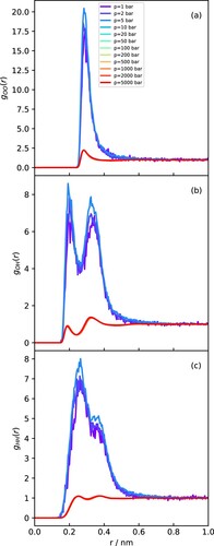
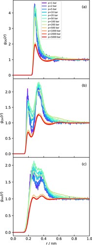
Figure 9. RDFs obtained at 700 K with varying pressures for (a) OO. (b) OH and (c) HH.

At 298 K, the system is in the liquid state at all of the pressure points studied, and the RDFs (Figure 7) exhibit the familiar signatures of the tetrahedral hydrogen bonded network of water [65]. As observed for the density, increasing pressure has a minor effect on the water structure until about 1000 bar. Above this pressure, the structure of the second solvation shell begins to change, essentially being pulled inwards, which results in a clear flattening of the second and third peaks of the OO RDF (Figure 7(a)) and a shift in the oscillations of the OH RDF (Figure 7(b)) [66].

Following the isotherm at 500 K (Figure 8), we can now see the abrupt transition from vapour to liquid as pressure increases. The liquid RDFs are qualitatively similar to those at 298 K, but the vapour-phase RDFs show only the signatures of first-neighbour interactions, with no structure beyond distances of about 0.5 nm. Notice that the peaks in the vapour phase appear much larger because the RDFs are normalised by the average bulk density, which is orders of magnitude lower in the vapour than in the liquid.

Finally, the RDFs at 700 K (Figure 9), corresponding to the transition from the gas to supercritical regimes, show much more gradual changes. At very low pressures, the structure is clearly gas-like, and the RDFs show a monotonic decay to 1 after the first neighbour peak(s). However, as the pressure increases, the RDFs develop oscillations at larger distances, eventually tending towards structures that are liquid-like at the highest pressures. The transition between a monotonic and an oscillatory decay of the OO RDFs determines the Fisher-Widom line, which marks the separation between gas-like and liquid-like states in the supercritical regime [39,67].

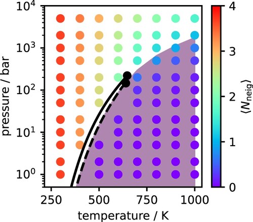
The variation in the water RDFs described above suggests that the degree of hydrogen bonding will also change with temperature and pressure in the supercritical regime. The change in the average number of hydrogen bonded neighbours per water molecule is shown in Figure 10 for all state points considered here, overlaid with the phase diagram. In general, as temperature increases and entropy plays a more significant role in dictating the structure of the system, the average number of hydrogen bonds decreases. This occurs gradually for pressures above the critical pressure; however, below the critical pressure, the number of hydrogen bonds reduces dramatically as water transitions from liquid to gas. At supercritical conditions, our simulations indicate the presence of hydrogen bonding between water molecules, but at significantly lower degree than in the liquid phase. Ai et al. also demonstrated this through classical molecular dynamics in the development of a reactive force field method [68]. We do note that our analysis is purely static in nature (i.e. based on analysing snapshots of the MD trajectory) and does not take into account the hydrogen bond dynamics, as done elsewhere [18,20].

Figure 10. Average number of hydrogen bonded neighbours $〈N\mathrm{neig}〉$ per water molecule. The shaded region denotes conditions where the $〈N\mathrm{neig}〉\le 1$.

In Figure 11, we plot the SCEE dipole moment as a function of the average number of H-bonded neighbours for each state point. When plotted this way, all points closely collapse into a single line, demonstrating a near linear relationship between the two properties. Schienbein and Marx [39] presented a similar linear relationship along the supercritical isotherm at 750 K, but our results indicate that this feature applies across a wide range of temperatures and pressures that span the vapour, liquid and supercritical phases. In other words, the dipole moment of water is almost entirely determined by the number of hydrogen bonds formed, and this phenomenon is the same in all phases and is largely independent of pressure and temperature (at least within the range considered here). The line of best fit in Figure 11 is $\mu \approx {\mu }_0+0.256〈N_{\mathrm{neig}}〉$, where ${\mu }_0=1.856$ D is the gas phase dipole moment. The slope of the line suggests that each additional hydrogen bond contributes about 0.25 D to the induced dipole moment, such that for the room temperature liquid (which has about 3.75 hydrogen bonds per molecule), the induced dipole moment is close to 2.8 D. In Figure 12, we compare the SCEE dipole moments with those calculated using the IEFPCM dielectric continuum model, where the dielectric constant of the surrounding medium was taken as the experimental value at each temperature and pressure of interest [63,69]. At low values of the dipole moment, corresponding to gas-like configurations, the predictions of both methods are in good agreement. 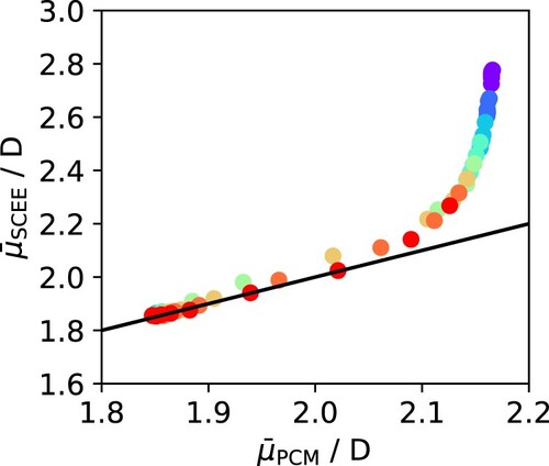However, as the dipole moment exceeds $\sim 2.1$ D, the two methods diverge, with SCEE predicting a much higher value of the dipole moment than the mean-field IEFPCM approach. Interestingly, it has previously been argued that a dipole moment of $\sim 2$ D marks the transition between H-bonded and non-H-bonded molecules [19,37]. To analyse this in more detail, the IEFPCM dipole moments were also plotted as a function of the number of hydrogen bonded neighbours in Figure 11. At very low number of H-bonds per molecule, the IEFPCM dipole moments are aligned with the SCEE predictions and increase nearly linearly. However, beyond a threshold of about 1 H-bond per molecule, the continuum predictions level off and appear to reach saturation, such that the dipole moment never exceeds 2.2 D. This can be explained if we consider that dielectric continuum models describe solvation effects in a mean-field manner and do not account for any local contributions to polarisation. In contrast, SCEE is designed to account for both local and mean field contributions, since it describes the solvent as being composed of discrete molecules that can interact with the central molecule and extends to large enough distances to recover bulk behaviour. As we have shown previously for water and alcohols [30,40], mean field and local effects contribute almost equally to molecular polarisation in hydrogen-bonding liquids at ambient conditions, with a slight dominance of the latter. However, for liquids that do not form hydrogen bonds, like ketones, the extent of polarisation can be reasonably predicted by considering mean field effects alone [41]. The present results show that these considerations can be generalised to a wide range of conditions, and that there is a clear threshold beyond which mean field effects are not sufficient to describe polarisation. For water, this threshold seems to occur at around 1 H-bond per molecule. Based on the data from our hydrogen bond analysis, we have found this threshold for each isotherm and marked it as a shaded area in the phase diagram of Figure 10. Interestingly, it follows on smoothly from the critical point, which suggests this might be another useful criterion for distinguishing between gas-like and liquid-like behaviour in the supercritical regime – akin to other widely discussed criteria such as the Fischer-Widom line [67], the Frenkel line [70], the Widom line [71], and the percolation line [72].

Figure 11. Variation of the average dipole moment with the number of nearest hydrogen bonded neighbours per water molecule, as computed by the SCEE method (full circles) and the IEFPCM method (open circles). The points are colour-coded by temperature as in Figure 2. The black line is a linear fit to the SCEE data.

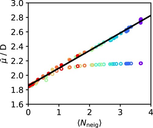
Figure 12. Comparison between the dipole moments calculated with SCEE and those obtained with the IEFPCM dielectric continuum model. The black line shows the diagonal corresponding to equality between both calculations. The points are colour-coded by temperature as in Figure 2.

4. Conclusions

In this work, we have calculated the molecular dipole moment of water over a wide range of thermodynamic conditions, including the vapour, liquid, and supercritical regimes. This was only possible through the application of our recently developed SCEE method, which allows for accurate dipole moment values to be obtained with modest computational expense [30,40]. Our results confirm that the dipole moment of liquid water is significantly enhanced relative to the gas phase value. The induced dipole is $\sim 0.9$ D at ambient conditions, but decreases gradually with temperature, such that it is only $\sim 0.5$ D close to the critical temperature. Interestingly, the width of the dipole moment distributions is practically independent of temperature, at least in the range considered here. Pressure has a comparatively smaller effect on the dipole moment; in fact, the liquid dipole seems to be nearly independent of pressure until about 1000 bar, beyond which a gradual increase is observed.

As the liquid state is approached from the vapour, there is a discontinuous change in the dipole moment, reflecting the underlying first-order phase transition. In marked contrast, the dipole moment distribution evolves continuously along supercritical isotherms – starting from a sharp gas-like peak at low T, the distributions develop a tail as the temperature increases, which then transforms into a separate peak as liquid-like densities are approached. Interestingly, there is still some overlap between dipole moment distributions for high-density and low-density supercritical states. In other words, dense supercritical states exhibit some molecular configurations that, at least from the perspective of polarisation, can still be considered gas-like.

Our analysis shows that the average water dipole moment calculated from SCEE depends linearly on the average number of hydrogen-bonded neighbours at each thermodynamic state point. At least for the range of T and P considered here, this relationship appears to be general, covering the vapour, liquid and supercritical regions. In contrast, dipole moments calculated from a dielectric continuum model do not show the same dependence. When, on average, a water molecule has more than $\sim 1$ hydrogen-bonded neighbour, the dielectric continuum model significantly underestimates the extent of polarisation, leading to dipole moments that are up to 50% lower than the SCEE estimates. This is because continuum models can only describe mean-field contributions to polarisation, whereas SCEE accounts for both mean-field and local contributions. In condensed phases of water, including both liquid and supercritical states, the latter play a very important role in the overall polarisation, hence cannot be neglected. We suggest that the point at which local (i.e. H-bond) contributions to polarisation start to become important can be used as a proxy to separate gas-like from liquid-like states in the supercritical regime.

We believe our work sheds new light on the properties of supercritical water, particularly on how the degree of polarisation, and hence the solvation properties, can be controlled by changing the temperature and pressure. Information on the molecular dipole moment in condensed phases is also extremely valuable to interpret and predict dielectric properties. For instance, we have shown previously that knowledge of the liquid-phase dipole moment can be used to eliminate systematic deviations in dielectric constant predictions from classical non-polarisable models through a post facto correction [24,73]. We are currently working on extending that approach to supercritical states, and plan to report on our findings in due course. Our results also have implications on how classical force fields are parameterised. For example, the dipole moment distributions we calculated can be used as targets for the development of polarisable water models, or to determine the optimal point charges for non-polarisable models [74]. Finally, it would be interesting to extend the present study to other molecules of different degrees of polarity (e.g. polar molecules without hydrogen-bonding capabilities) to determine to which extent the conclusions presented herein are generalisable.

Disclosure statement

No potential conflict of interest was reported by the author(s).

Data Availability Statement

All data underpinning this publication are openly available from the University of Strathclyde KnowledgeBase at doi: 10.15129/75e6fe2b-5575-449e-8af4-007558ba1b3b

 Google Scholar

.

Additional information

Funding

ZM acknowledges EPSRC for a Doctoral Training Grant, ref EP/W524670/1. JRBG thanks project CICECO-Aveiro Institute of Materials, UIDB/50011/2020, UIDP/50011/2020 and LA/P/0006/2020, financed by national funds through the FCT/MEC (PIDDAC) and the COST Action 18234.

References

- T.I. Mizan, P.E. Savage and R.M. Ziff, J. Comput. Chem. 17 (15), 1757–1770 (1996). doi:10.1002/(ISSN)1096-987X
- M. Fugel and V.C. Weiß, J. Chem. Phys. 146 (6), 064505 (2017). doi:10.1063/1.4975778
- P. Ball, Nature 452 (7185), 291–292 (2008). doi:10.1038/452291a
- J. Russo and H. Tanaka, Nat. Commun. 5 (1), 3556 (2014). doi:10.1038/ncomms4556
- J.R. Errington and P.G. Debenedetti, Nature 409 (6818), 318–321 (2001). doi:10.1038/35053024
- J.L. Finney, J. Chem. Phys. 160 (6), 060901 (2024). doi:10.1063/5.0182665
- L.G.M. Pettersson, R.H. Henchman and A. Nilsson, Chem. Rev. 116 (13), 7459–7462 (2016). doi:10.1021/acs.chemrev.6b00363
- H. Weingärtner and E.U. Franck, Angew. Chem. Int. Ed. 44 (18), 2672–2692 (2005). doi:10.1002/anie.v44:18
- P. Sun, J.B. Hastings, D. Ishikawa, A.Q.R. Baron and G. Monaco, Phys. Rev. Lett. 125 (25), 256001 (2020). doi:10.1103/PhysRevLett.125.256001
- P.E. Savage, Chem. Rev. 99 (2), 603–622 (1999). doi:10.1021/cr9700989
- K. Khandelwal, S. Nanda, P. Boahene and A.K. Dalai, Environ. Chem. Lett. 21 (5), 2619–2638 (2023). doi:10.1007/s10311-023-01624-z
- R.F. Susanti, L.W. Dianningrum, T. Yum, Y. Kim, Y.W. Lee and J. Kim, Chem. Eng. Res. Des. 92 (10), 1834–1844 (2014). doi:10.1016/j.cherd.2014.01.003
- F.J.G. Ortiz and A. Kruse, React. Chem. Eng. 5 (3), 424–451 (2020). doi:10.1039/C9RE00465C
- Y. Marcus, Separations 5 (1), 4 (2018). doi:10.3390/separations5010004
- K.Y. Khaw, M.O. Parat, P.N. Shaw and J.R. Falconer, Molecules 22 (7), 1186 (2017). doi:10.3390/molecules22071186
- A.L.B. Dias, A.C. de Aguiar and M.A. Rostagno, Ultrason. Sonochem. 74, 105584 (2021). doi:10.1016/j.ultsonch.2021.105584
- J.A. Okolie, R. Rana, S. Nanda, A.K. Dalai and J.A. Kozinski, Sustain. Energ. Fuels 3 (3), 578–598 (2019). doi:10.1039/C8SE00565F
- A. Karmakar and A. Chandra, ACS Omega 3 (3), 3453–3462 (2018). doi:10.1021/acsomega.7b02036
- O.V. Ved, D.L. Gurina, M.L. Antipova and V.E. Petrenko, Russ. J. Phys. Chem. A 84 (8), 1359–1363 (2010). doi:10.1134/S0036024410080157
- P. Schienbein and D. Marx, Angew. Chem. Int. Ed. 59 (42), 18578–18585 (2020). doi:10.1002/anie.v59.42
- I. Leontyev and A. Stuchebrukhov, Phys. Chem. Chem. Phys. 13 (7), 2613–2626 (2011). doi:10.1039/c0cp01971b
- A.W. Milne and M. Jorge, J. Chem. Theory Comput. 15 (2), 1065–1078 (2019). doi:10.1021/acs.jctc.8b01115
- C. Vega, Mol. Phys. 113, 1145–1163 (2015). doi:10.1080/00268976.2015.1005191
- M. Jorge and L. Lue, J. Chem. Phys. 150 (8), 084108 (2019). doi:10.1063/1.5080927
- S.A. Clough, Y. Beers, G.P. Klein and L.S. Rothman, J. Chem. Phys. 59 (5), 2254–2259 (1973). doi:10.1063/1.1680328
- T. Zhu and T. Van Voorhis, J. Phys. Chem. Lett. 12 (1), 6–12 (2020). doi:10.1021/acs.jpclett.0c03300
- M. Born, Z. Phys. 1 (1), 45–48 (1920). doi:10.1007/BF01881023
- J.G. Kirkwood, J. Chem. Phys. 7 (10), 911–919 (1939). doi:10.1063/1.1750343
- L. Onsager, J. Am. Chem. Soc. 58 (8), 1486–1493 (1936). doi:10.1021/ja01299a050
- M. Jorge, J.R.B. Gomes and A.W. Milne, J. Mol. Liq. 322, 114550 (2021). doi:10.1016/j.molliq.2020.114550
- C.A. Coulson and D. Eisenberg, Proc. R. Soc. Lond. A Math. Phys. Sci. 291 (1427), 445–453 (1997).
- Y.S. Badyal, M.L. Saboungi, D.L. Price, S. Shastri, D.R. Haeffner and A.K. Soper, J. Chem. Phys.112 (21), 9206–9208 (2000). doi:10.1063/1.481541
- A.V. Gubskaya and P.G. Kusalik, J. Chem. Phys. 117 (11), 5290–5302 (2002). doi:10.1063/1.1501122
- P.L. Silvestrelli and M. Parrinello, Phys. Rev. Lett. 82 (16), 3308–3311 (1999). doi:10.1103/PhysRevLett.82.3308
- H.M. Senn and W. Thiel, Angew. Chem. Int. Ed. 48 (7), 1198–1229 (2009). doi:10.1002/anie.v48:7
- M. Boero, K. Terakura, T. Ikeshoji, C.C. Liew and M. Parrinello, Phys. Rev. Lett. 85 (15), 3245–3248 (2000). doi:10.1103/PhysRevLett.85.3245
- M. Boero, K. Terakura, T. Ikeshoji, C.C. Liew and M. Parrinello, J. Chem. Phys. 115 (5), 2219–2227 (2001). doi:10.1063/1.1379767
- D. Kang, J. Dai and J. Yuan, J. Chem. Phys. 135 (2), 024505 (2011). doi:10.1063/1.3608412.
- P. Schienbein and D. Marx, J. Phys. Chem. Chem. Phys. 22, 10462–10479 (2020). doi:10.1039/C9CP05610F
- M. Jorge, J.R.B. Gomes and M.C. Barrera, J. Mol. Liq. 356, 119033 (2022). doi:10.1016/j.molliq.2022.119033
- M.C. Barrera, J. Cree, J.R.B. Gomes and M. Jorge, J. Mol. Liq. 383, 122070 (2023). doi:10.1016/j.molliq.2023.122070
- H.J.C. Berendsen, D. van der Spoel and R. van Drunen, Comput. Phys. Commun. 91 (1), 43–56 (1995). doi:10.1016/0010-4655(95)00042-E
- M.J. Abraham, T. Murtola, R. Schulz, S. Páll, J.C. Smith, B. Hess and E. Lindahl, SoftwareX1-2, 19–25 (2015). doi:10.1016/j.softx.2015.06.001
- R.W. Hockney, S.P. Goel and J.W. Eastwood, J. Comput. Phys. 14 (2), 148–158 (1974). doi:10.1016/0021-9991(74)90010-2
- G. Bussi, D. Donadio and M. Parrinello, J. Chem. Phys. 126 (1), 014101 (2007). doi:10.1063/1.2408420
- M. Parrinello and A. Rahman, Phys. Rev. Lett. 45 (14), 1196–1199 (1980). doi:10.1103/PhysRevLett.45.1196
- J.L.F. Abascal and C. Vega, J. Chem. Phys. 123 (23), 234505 (2005). doi:10.1063/1.2121687
- C. Vega and J.L.F. Abascal, Phys. Chem. Chem. Phys. 13 (44), 19663–19688 (2011). doi:10.1039/c1cp22168j
- C. Vega, J.L.F. Abascal and I. Nezbeda, J. Chem. Phys. 125 (3), 034503 (2006). doi:10.1063/1.2215612
- B. Hess, H. Bekker, H.J.C. Berendsen and J.G.E.M. Fraaije, J. Comput. Chem. 18 (12), 1463–1472 (1997). doi:10.1002/(ISSN)1096-987X
- T. Darden, D. York and L. Pedersen, J. Chem. Phys. 98 (12), 10089–10092 (1993). doi:10.1063/1.464397
- V. Shen, D. Sideriu, W. Krekelberg and H. Hatch, NIST Standard Reference Database Number 173, vols. 20899 (National Institute of Standards and Technology, Gaithersburg, MD, 2014).
- K. Coutinho, R.C. Guedes, B.J.C. Cabral and S. Canuto, Chem. Phys. Lett. 369 (3), 345–353 (2003). doi:10.1016/S0009-2614(02)02026-2
- M.J. Frisch, G.W. Trucks, H.B. Schlegel, G.E. Scuseria, M.A. Robb, J.R. Cheeseman, G. Scalmani, V. Barone, G.A. Petersson, H. Nakatsuji, M. Caricato, X. Li, H.P. Hratchian, A.F. Izmaylov, J. Bloino, G. Zheng, J.L. Sonnenberg, M. Hada, M. Ehara, K. Toyota, R. Fukuda, J. Hasegawa, M. Ishida, T. Nakajima, Y. Honda, K. Kitao, H. Nakai, T. Vreven, J.A. Montgomery, Jr., J.E. Peralta, F. Ogliaro, M. Bearpark, J.J. Heyd, E. Brothers, K.N. Kudin, V.N. Staroverov, R. Kobayashi, J. Normand, K. Raghavachari, A. Rendell, J.C. Burant, S.S. Iyengar, J. Tomasi, M. Cossi, N. Rega, J.M. Millam, M. Klene, J.E. Knox, J.B. Cross, V. Bakken, C Adamo, J. Jaramillo, R. Gomperts, R.E. Stratmann, O. Yazyev, A.J. Austin, R. Cammi, C. Pomelli, J.W. Ochterski, R.L. Martin, K. Morokuma, V.G. Zakrzewski, G.A. Voth, P. Salvador, J.J. Dannenberg, S. Dapprich, A.D. Daniels, O. Farkas, J.B. Foresman, J.V. Ortiz, J. Cioslowski and D.J. Fox, Gaussian 09, Revision B.01 (Gaussian, Inc., Wallingford, CT, 2009).
- F. Maseras and K. Morokuma, J. Comput. Chem. 16 (9), 1170–1179 (1995). doi:10.1002/jcc.v16:9
- S. Dapprich, I. Komáromi, K.S. Byun, K. Morokuma and M.J. Frisch, J. Mol. Struct. 461-462, 1–21 (1999). doi:10.1016/S0166-1280(98)00475-8
- C. Lee, W. Yang and R.G. Parr, Phys. Rev. B Condens. Matter 37 (2), 785–789 (1988). doi:10.1103/PhysRevB.37.785
- A.D. Becke, J. Chem. Phys. 98 (7), 5648–5652 (1993). doi:10.1063/1.464913
- T.H. Dunning, Jr., J. Chem. Phys. 90 (2), 1007–1023 (1989). doi:10.1063/1.456153
- A.L. Hickey and C.N. Rowley, J. Phys. Chem. A 118 (20), 3678–3687 (2014). doi:10.1021/jp502475e
- D. Hait and M. Head-Gordon, J. Chem. Theory Comput. 14 (4), 1969–1981 (2018). doi:10.1021/acs.jctc.7b01252
- E. Cancès, B. Mennucci and J. Tomasi, J. Chem. Phys. 107 (8), 3032–3041 (1997). doi:10.1063/1.474659
- D.P. Fernández, A.R.H. Goodwin, E.W. Lemmon, J.M.H. Levelt Sengers and R.C. Williams, J. Phys. Chem. Ref. Data 26 (4), 1125–1166 (1997). doi:10.1063/1.555997
- H. Sakuma, M. Ichiki, K. Kawamura and K. Fuji-ta, J. Chem. Phys. 138 (13), 134506 (2013). doi:10.1063/1.4798222
- A. Soper, Chem. Phys. 258 (2–3), 121–137 (2000). doi:10.1016/S0301-0104(00)00179-8
- A.K. Soper and M.A. Ricci, Phys. Rev. Lett. 84 (13), 2881–2884 (2000). doi:10.1103/PhysRevLett.84.2881
- M.E. Fisher and B. Widom, J. Chem. Phys. 50 (9), 3756–3772 (1969). doi:10.1063/1.1671624
- L. Ai, Y. Zhou and M. Chen, J. Mol. Liq. 276, 83–92 (2019). doi:10.1016/j.molliq.2018.11.133
- D.P. Fernández, Y. Mulev, A.R.H. Goodwin and J.M.H.L. Sengers, J. Phys. Chem. Ref. Data 24 (1), 33–70 (1995). doi:10.1063/1.555977
- V.V. Brazhkin, Y.D. Fomin, A.G. Lyapin, V.N. Ryzhov and K. Trachenko, Phys. Rev. E 85, 031203 (2012). doi:10.1103/PhysRevE.85.031203
- L. Xu, P. Kumar, S.V. Buldyrev, S.H. Chen, P.H. Poole, F. Sciortino and H.E. Stanley, Proc. Natl. Acad. Sci. USA 102 (46), 16558–16562 (2005). doi:10.1073/pnas.0507870102
- L. Pártay and P. Jedlovszky, J. Chem. Phys. 123 (2), 024502 (2005). doi:10.1063/1.1953547
- J. Cardona, M. Jorge and L. Lue, Phys. Chem. Chem. Phys. 22 (38), 21741–21749 (2020). doi:10.1039/D0CP04034G
- M. Jorge, M.C. Barrera, A.W. Milne, C. Ringrose and D.J. Cole, J. Chem. Theory Comput. 19 (6), 1790–1804 (2023). doi:10.1021/acs.jctc.2c01123