An Introduction to Network Psychometrics: Relating Ising Network Models to Item Response Theory Models

ABSTRACT

In recent years, network models have been proposed as an alternative representation of psychometric constructs such as depression. In such models, the covariance between observables (e.g., symptoms like depressed mood, feelings of worthlessness, and guilt) is explained in terms of a pattern of causal interactions between these observables, which contrasts with classical interpretations in which the observables are conceptualized as the effects of a reflective latent variable. However, few investigations have been directed at the question how these different models relate to each other. To shed light on this issue, the current paper explores the relation between one of the most important network models—the Ising model from physics—and one of the most important latent variable models—the Item Response Theory (IRT) model from psychometrics. The Ising model describes the interaction between states of particles that are connected in a network, whereas the IRT model describes the probability distribution associated with item responses in a psychometric test as a function of a latent variable. Despite the divergent backgrounds of the models, we show a broad equivalence between them and also illustrate several opportunities that arise from this connection.

KEYWORDS:

• Psychometrics
• network model
• latent variable model
• Rasch model

Introduction

The question of how observables (e.g., behaviors, responses to questionnaire items, or cognitive test performance) should be related to theoretical constructs (e.g., attitudes, mental disorders, or intelligence) is central to the discipline of psychometrics (Borsboom & Molenaar, 2015). Despite the wide variety of constructs covered in psychometric work and the great flexibility of mathematical representations, however, the collection of relations between constructs and behaviors that have been envisaged in psychometric models is surprisingly limited. We can think of four ways in which this connection between constructs and observations has been construed.

First, theoretical constructs have been conceptualized as inductive summaries of attributes or behaviors as displayed by a person (Cronbach & Meehl, 1955). For instance, one could count the total number of times a researcher has been cited and label this quantity “scientific impact.” This characterization attaches a verbal label to an overall summary of observable features of a person, but does not explicitly involve inference to an underlying attribute; it simply recodes the observations in a useful way. The statistical model most often associated with this idea is the Principal Component Analysis (PCA) model (Pearson, 1901), which offers a systematic method of constructing a weighted sumscore that summarizes the variance in the observables. Importantly, such data-reductive models do not typically involve an inference that goes beyond the information present in the observations (i.e., if one knows the observations and the model, one knows the component scores).

Second, theoretical constructs have been conceived of as behavior domains (also called universes of behaviors). In this interpretation, a construct such as, say, “addition ability” is conceptualized as a measure on the domain of addition (the so-called behavior domain; McDonald, 2003); for instance, as the total number of all possible addition items that a person can solve. An addition test may then be constructed as a finite sample of items from this domain. Thus, in this case the construct could also be seen as an inductive summary (namely, of the behavior domain), but it does not coincide with the test score. This is because the test score captures some, but not all of the observables that constitute the behavior domain. The required inductive inference from test score to construct is then typically considered a species of statistical generalization (Markus & Borsboom, 2013), and the model most naturally associated with this idea is that of Generalizability Theory (Brennan, 2001; Cronbach, Rajaratnam, & Gleser, 1963; Cronbach, Gleser, Harinder, & Rajaratnam, 1972), although under certain assumptions this conceptualization can also imply a latent variable model (Ellis & Junker, 1997; McDonald, 2003).

Third, theoretical constructs have been viewed as common effects of a set of observable features. For example, Bollen and Lennox (1991) give the example of life stress, which may be assessed by recording the number of stressful events that a person has experienced in the past year. The assumption that underwrites this approach is that more stressful events generate more psychological stress (the theoretical construct of interest), so that the number of experienced events can function as a proxy for a person’s experienced stress. Models associated with this idea are known as formative models (Edwards & Bagozzi, 2000). In the statistical model that this conceptualization motivates, a latent variable is regressed on a set of observables to statistically encode the assumption that the observables cause the latent variable. Thus, in formative models, the relation between indicators and construct is causal, and the inference characterizing the measurement process could be characterized as forward causal inference, that is, from causes to effects.

Fourth, theoretical constructs have been considered to be the common cause of observable behaviors. This conception could in fact be considered to be the first psychometric theory, as it coincides with the birth of psychometric modeling: the postulation by Spearman (1904) that the variance in cognitive test scores is causally determined by the pervasive influence of general intelligence. A corollary of this theory is that we can infer a person’s level of general intelligence from his or her performance on a set of cognitive tests. The idea that we learn about a person’s standing on an attribute like general intelligence by exploiting the causal relation between that attribute and our measures, is known as reflective measurement. The conceptualization offered in reflective measurement is, we think, currently the most widely espoused theory among psychologists working in fields like intelligence, personality, and attitude research. Importantly, in this model, the relation between the theoretical construct and its psychometric indicator is considered to be causal, which implies that measurement is a species of causal inference, as it is in the formative case—however, in contrast to the formative case, here the inference is backward (from effects to causes). The statistical model most often associated with reflective model is the common factor model (Bollen & Lennox, 1991; Edwards & Bagozzi, 2000), although Item Response Theory (IRT) models have also been interpreted reflectively (Waller & Reise, 2010).

The models mentioned above have in some form or another, all been around for at least half a century, and it may seem that they exhaust the conceptual possibilities for relating observables to theoretical constructs. This, however, is not the case. Recently, a fifth conceptual model has been added to the pantheon of psychometric theories on the relation between constructs and observations, namely, the network model (Borsboom, 2008; Borsboom & Cramer, 2013; Cramer, Waldorp, van der Maas, & Borsboom, 2010). The idea that underlies this model, first articulated by van der Maas et al. (2006) is that observable features (e.g., symptoms of depression) may form a network of mutually reinforcing entities connected by causal relations. In this case, the relation between construct and observables is mereological (a part-whole relation) rather than causal (the observables are part of the construct, but do not stand in a causal relation to it). Although network models can be constructed in many ways, the class of statistical models that has become associated with these models in the past few years is the class of graphical models, in which variables are represented as nodes, while (the absence of) edges between nodes encode (the absence of) conditional associations between nodes (Lauritzen, 1996).

In the current paper, we study the relation between network models and existing psychometric models on the relation between constructs and observations, most importantly, the reflective latent variable model. As will become apparent, even though the conceptual framework that motivates the statistical representation in a psychometric model may be strikingly different for network models and latent variable models, the network models and latent variable models turn out to be strongly related; so strongly, in fact, that we are able to establish a general correspondence between the model representations and, in certain cases, full statistical equivalence. This allows us to open up a surprising connection between one of the most intensively studied network models in physics—namely, the Ising (1925) model—and one of the most intensively studied latent variable models—namely, the Item Response Theory (IRT) model (e.g., Embretson & Reise, 2000; Mellenbergh, 1994; van der Linden & Hambleton, 1997). This opens up a new field of research in psychometrics, and offers a novel way of looking at theories of psychological measurement.^{Figure 1}

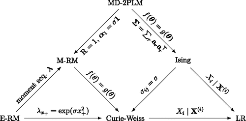
Our primary aim is to organize the results about the relations between network models and latent variable models, and to study these relations from a psychometric point of view. The structure of this paper is as follows. First, we explain the logic of network models, starting from the original formulation of the Ising model. Second, we show that a particular restricted form of the Ising model—namely, the Curie-Weiss model (Kac, 1968)—is statistically equivalent to a particular class of Rasch (1960) models, known as the family of extended Rasch models (E-RMs; Tjur, 1982) and, specifically, the marginal Rasch model (M-RM; Bock & Aitken, 1981). Third, we establish a broad connection between multidimensional IRT models, specifically the multidimensional two-parameter logistic model (MD-2PLM; Reckase, 2009), and Ising models defined on an arbitrary network topology. In these two sections, we will detail the theory connecting the statistical models that are shown in Figure 1 and illustrate this theory with new insights that are relevant to existing psychometric theory. Finally, we discuss new perspectives on general psychometric problems that arise from this work and illustrate what the model equivalence means in practice.

Figure 1. A network of statistical models with the edges showing equivalence relation between the models subject to the constraints given on the edge labels. The edges are directed and originate from the more general model. The nodes refer to the extended Rasch model (E-RM), marginal Rasch model (M-RM), multidimensional two-parameter logistic model (MD-2PLM), Ising model (Ising), Curie-Weiss model (Curie-Weiss), and Logistic regression (LR).

The Ising network model from theoretical physics

The main character in our story is a theoretical model that was introduced nearly a century ago in the physics literature (Lenz, 1920) to describe the orientation of particles that are placed on a square grid called a lattice graph (e.g., Brush, 1967; Niss, 2005). Figure 2 shows such a lattice graph, which is a simple network that consists of n nodes (circles) with edges (solid lines) between adjacent nodes. Each node on the lattice graph represents a particle that has a spin x_i, i = 1, …, n, that is restricted to either point up “↑” or point down “↓”. These spin random variables are typically coded as x_i = +1 for “↑” and x_i = −1 for “↓”.¹ That is, the model that was introduced by Lenz (1920), and further studied by his student Ising (1925), describes a nearest neighbor network of binary random variables: (1) where the sum ∑_{< i, j >} ranges over all node pairs (i, j) that are direct neighbors on the lattice graph, which are indicated with solid lines in Figure 2, and ∑_x is the sum over all 2ⁿ possible configurations x = (x₁, …, x_n) of n spins. The spins tends to point upward (x_i = +1) when their main effects are positive (μ_i > 0) and downward (x_i = −1) when their main effects are negative (μ_i < 0). Furthermore, any two spins x_i and x_j that are direct neighbors on the lattice graph tend to be in the same state when their interaction effect is positive (σ_ij > 0) and tend to be in different states when their interaction is negative (σ_ij < 0). This model is now known as the Ising model, although some refer to it as the Lenz-Ising model (e.g., Brush, 1967; Niss, 2005, 2009, 2011).

Figure 2. A square 3 × 3 lattice where the nodes (circles) refer to the upward “↑” or downward “↓” orientation of particles, and it is assumed that the particles only interact with their nearest neighbors (indicated with solid lines).

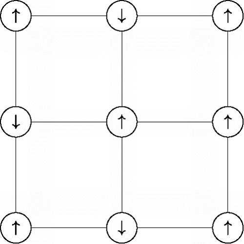
From a statistical perspective, the Ising model is a simple nontrivial network model involving main effects and pairwise interactions. Despite its simplicity, the Ising model is well known for its ability to describe complex phenomena that originate from its local interactions. With an estimated 800 papers written about the Ising model every year (Stutz & Williams, 1999), it has become one of the most influential models from statistical physics, finding applications in such diverse fields as image restoration (Geman & Geman, 1984), biology (Fierst & Phillips, 2015), sociology (Galam, Gefen, & Shapir, 1982; Galam & Moscovici, 1991), and more recently psychology (Epskamp, Maris, Waldorp, & Borsboom, in press) and educational measurement (Marsman, Maris, Bechger, & Glas, 2015). For instance, the spins may refer to the presence or absence of symptoms in psychopathology, and to the correct or incorrect answers to items in an educational test.

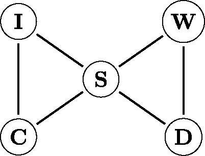
To illustrate the model, we consider a simple example from the psychopathology literature. In Figure 3, we show a network of a selection of major depression (MD) and generalized anxiety disorder (GAD) symptoms, which are taken from the fourth edition of the Diagnostic and Statistical Manual of Mental Disorders (DSM-IV; the complete n = 15 variable network is shown in Borsboom & Cramer, 2013). The network in Figure 3 consists of two cliques of three symptoms: the GAD symptoms irritability (I), chronic worrying (C), and sleep problems (S) form one clique and the MD symptoms weight problems (W), depressed mood (D) and sleep problems (S) form another. The symptom sleep problems (S) is shared between the two disorders/cliques, which is known as a so-called bridge symptom. Note that the two unique GAD symptoms (I and C) have no immediate link to the two MD symptoms (D and W), indicating that chronic worry (C) affects having a depressed mood (D) only indirectly via the bridge symptom sleep problems (S). Thus, the two unique GAD symptoms are independent of the unique MD symptoms conditional upon the bridge symptom (S), as indicated in Figure 3 by an absence of edges connecting these variables.

Figure 3. A network of five selected major depression (MD) and generalized anxiety disorder (GAD) symptoms that are taken from the fourth edition of the Diagnostic and Statistical Manual of Mental Disorders (DSM-IV; a complete version of this network is shown in Borsboom & Cramer, 2013). Irritability (I) and chronic worrying (C) are GAD symptoms, weight problems (W) and depressed mood (D) are MD symptoms, and sleep problems (S) is a symptom of both MD and GAD.

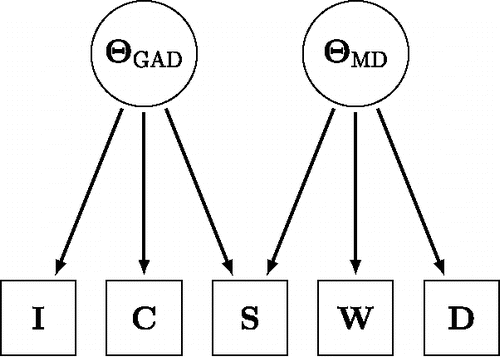
The (Ising) network model differs markedly from the common cause model that is traditionally used in psychopathology, which represents the observed dependence and independence relations using latent variables (Borsboom, 2008). Such a latent variable representation for the five variable symptom network is shown in Figure 4 and assumes the existence of two latent variables; one for GAD and one for MD. The primary distinction between the two conceptual models that are shown in Figures 3 and 4 is in what causes the variations in the observables (e.g., symptoms, item scores). Whereas the common cause model suggests that a person develops a symptom because he or she is depressed, the direct interaction model suggests that a symptom develops under the influence of other symptoms or (observable) external factors.

Figure 4. A common cause representation of the manifest relations between GAD and MD symptoms in Figure 3.

Despite the fact that these conceptual models differ markedly in their interpretation as to what causes covariances in observables, it has been previously noted that the associated statistical models are closely related. For example, Cox and Wermuth (2002) showed that there is an approximate relation between the Ising model, or quadratic exponential distribution (Cox, 1972), and the IRT model of Rasch (1960). Moreover, Molenaar (2003, p. 82) specifically suggested that there exists a formal connection between the Ising model and the IRT models of Rasch and Birnbaum (1968). This formal connection between the Ising model and IRT models was recently established and it is the aim of the present paper to detail this connection. We first consider a simplest nontrivial case; the fully connected Ising model and its connection to a one-factor latent variable model.

The Curie-Weiss and Rasch models

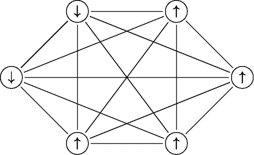
The Ising model’s success in physics is due to the fact that it is one of the simplest models that exhibits a phase transition (shifting from one state of matter to another; Brout, 1968). However, the study of phase transitions with the Ising model proved to be very difficult and enticed the study of phase transitions in even simpler models. Most notable is the Curie-Weiss model (Kac, 1968; Kochmański, Paskiewicz, & Wolski, 2013), also known as the fully connected Ising model: (2) in which x₊ = ∑ⁿ_{i = 1}x_i refers to the sum of the node states, that is, it is the analog of a total test score in psychometrics. Whereas the Ising model allows the interaction strength σ_ij to vary between node-pairs, most notably that σ_ij = 0 whenever node i and j are no direct neighbors in Figure 2, the Curie-Weiss model assumes that there is a constant interaction σ > 0 between each pair of nodes, which induces a network such as that shown in Figure 5.

Figure 5. A graphical representation of the Curie-Weiss network. The nodes (circles) refer to the upward “↑” and downward “↓” orientation of particles and each particle interacts with each other particle (solid lines).

From a psychometric perspective, it is clear that the relations in Figure 5 also correspond to a model with a single latent variable. From this perspective, it is interesting to observe that the Curie-Weiss model is closely related to the extended-Rasch model (E-RM; Cressie & Holland, 1983; Tjur, 1982), a particular item response model originating from educational and psychological measurement (Anderson, Li, & Vermunt, 2007; Hessen, 2011; Maris, Bechger, & San Martin, 2015). In the E-RM, the distribution of n binary variables x—typically the scores of items on a test—is given by (3) where the β_i relate to the difficulties of items on the test and the to the probability of scoring 2x₊ − n out of n items correctly. It can be shown that the E-RM consists of two parts (e.g., Maris et al., 2015): a marginal probability characterizing the distribution of total scores x₊ (e.g., scores achieved by pupils on an educational test, or number of symptoms of subjects in a clinical population), and a conditional probability characterizing the distribution of the item scores/symptomatic states given that the total score was x₊. Comparing the expression for the Curie-Weiss model in Equation (2(2) ) and that for the E-RM in Equation (3(3) ), we see that they are equivalent subject to the constraints: That is, whenever a quadratic relation holds between the total scores x₊ and the log  of the parameters in the E-RM, the E-RM is equivalent to the Curie-Weiss model.

It seems that we have made little progress, as the expressions for both the Curie-Weiss model in Equation (2(2) ) and the E-RM in Equation (3(3) ) do not involve latent variables. This is not the case, however, as the E-RM has been studied in the psychometric literature mostly due to its connection to a latent variable model known as the marginal-Rasch model (M-RM; Bock & Aitken, 1981; Glas, 1989). Consider again Equation (2(2) ), and suppose that we obtain a latent variable that explains all connections in the Curie-Weiss model, such that the observations are independent given the latent variable: A particular example of such a conditional distribution is an IRT model known as the Rasch model² (Rasch, 1960): where the δ_i are commonly referred to as item difficulties. In the M-RM, the distribution of the n binary variables x is then expressed as (4) where f(θ) is a population or structural model for the latent variable θ (Adams et al., 1997). This structural model is typically assumed to be a normal distribution. It can be shown that the marginal probability p(x) given by the M-RM consists of the same two parts as the E-RM (e.g., de Leeuw & Verhelst, 1986), except that the marginal probability is modeled with a latent variable in the M-RM. Importantly, the E-RM simplifies to an M-RM if and only if the λ_s constitute a sequence of moments (Cressie & Holland, 1983; see Theorem 3 in Hessen, 2011, for the moment sequence of a normal structural model). This suggests that there exists an explicit relation between a one factor model (the unidimensional Rasch model) and the fully connected network in Figure 5.

Whereas the connection between the E-RM and the M-RM has been known for many decades, the connection between the Curie-Weiss model and the M-RM was only recently observed (Epskamp et al., in press; Marsman et al., 2015). The relation stems from an application of the Gaussian integral: Kac (1968) realized that the exponential of a square can be replaced by the integral on the right-hand side, and applied this representation to exp (σx²₊) in the expression for the Curie-Weiss model. 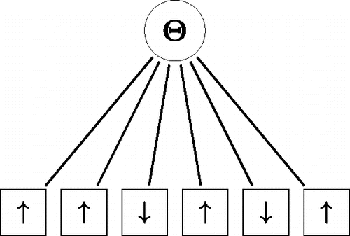We then only need a bit of algebra to obtain the M-RM in Equation (4(4) ), with δ_i = −μ_i.³ This is an important result as it implies the statistical equivalence of the network approach in Figure 5 and the latent variable approach in Figure 6.

Figure 6. A graphical representation of the Rasch model. The observables (squares) refer to the upward “↑” and downward “↓” orientation of particles and each particle interacts with another particle only through the latent variable Θ.

The structural model that results from the derivation is not the typically used normal distribution, but the slightly peculiar: where the posterior distribution g(θ∣x) is a normal distribution with mean 2σx₊ and variance 2σ. That is, g(θ) reduces to a mixture of n + 1 different normal (posterior) distributions; one for every possible test score. 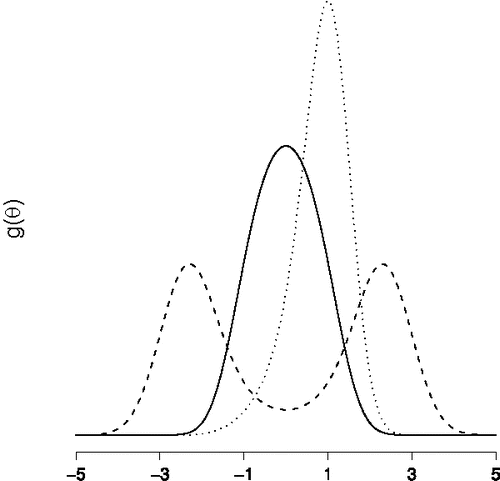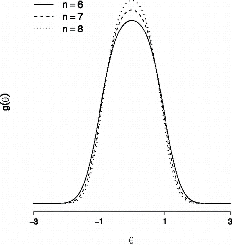In the graphical modeling literature, the joint distribution is known as a homogenous conditional Gaussian distribution (HCG; Lauritzen & Wermuth, 1989), a distribution that was first studied by Olkin and Tate (1961, see also; Tate, 1954, 1966). Some instances of the structural model are shown in Figure 7, which reveals a close resemblance to a mixture of two normal distributions with equal variances and their respective means placed symmetrically about zero. For an interaction effect σ that is sufficiently small, Figure 7 reveals that g(θ) is close to the typically used normal model.

Figure 7. Some instances of the structural model g(θ) for the n = 6 variable network. The solid line refers to the distribution with σ = 0.1 and the μ_i equally spaced between − 1 and + 1. The dashed line refers to the distribution with σ = 0.2 and the μ_i equally spaced between − 1 and + 1. The dotted line refers to the distribution with σ = 0.1 and the μ_i equally spaced between − 0.2 and + 1.

The relation between the Curie-Weiss model and the M-RM with structural model g(θ) has been established before in the psychometric literature on log-multiplicative association models (LMA; Anderson & Vermunt, 2000; Anderson & Yu, 2007; Anderson et al., 2007; Holland, 1990). However, it was not realized that the marginal distribution p(x) (i.e., the LMA model) was a Curie-Weiss model. In return, the Gaussian integral representation that was introduced by Kac (1968) has been used in physics to study the Curie-Weiss model (e.g., Emch & Knops, 1970), and has been independently (re-)discovered throughout the statistical sciences (Lauritzen & Wermuth, 1989; McCullagh, 1994; Olkin & Tate, 1961). Here, however, it was not realized that the conditional distribution p(x∣θ) is a Rasch model.

New insight I: The structural model g(θ) and psychometric theory

The structural model and the normal posterior distribution

Even though we have observed that g(θ) is close to the typically used normal structural model when σ is sufficiently small, or can be closely approximated using a mixture of two normal distributions otherwise (e.g., Marsman, Maris, & Bechger, 2012), the use of g(θ) as structural model leads to a qualitatively different marginal IRT model. For one thing, the item difficulty parameters δ_i are completely identified in the M-RM with g(θ) as structural model, something that cannot be said in the general case when using a (mixture of) normal distribution(s) for the structural model f(θ). Specifically, in a regular M-RM the item parameters δ only have their relative differences identified, but not their absolute value. It is clear that this observation has an immediate impact on the assessment of measurement invariance—differential item functioning (DIF) in the IRT literature—as the nonidentifiability imposes restrictions as to what can or cannot be assessed in DIF analyses (e.g., Bechger & Maris, 2015). However, that the structural model g(θ) leads to a qualitatively different marginal IRT model is most apparent in the simple analytically available normal posterior distribution it implies for the latent variable.

The idea of assuming posterior normality for the latent variable in the IRT literature can be traced back to a seminal paper by Paul Holland in 1990, which also initiated the study of LMA models in psychometrics. The topic of asymptotic posterior normality has subsequently been pursued by Chang and Stout (1993) and Chang (1996) (see also; Zhang & Stout, 1997). An important result is that if the number of variables (items) n tends to become very large, the posterior distribution converges to a normal distribution that is centered on the true value Θ₀ of the latent variable (e.g., Chang & Stout, 1993), and conditionally a strong law of large numbers: However, the posterior normal distribution g(θ∣x_n) that is implied by the structural model g(θ) does not have the property that it converges in the traditional manner, since the posterior variance is constant and does not decrease when n increases. Furthermore, the posterior expectations diverge as n grows, and it is unknown how a posterior distribution given n observations relates to a posterior distribution given n + 1 observations. It turns out that the study of the limiting behavior of the latent variable distribution, and in particular the structural model g(θ), is related to the study of the limiting behavior of networks for n → ∞—known as the thermodynamic limit in physics.

The posterior distribution g(θ∣x) and the study of its limit

Two difficulties arise in the study of thermodynamic limits. A first difficulty is that the network models are not nested in n. That is, for the Curie-Weiss model p(x) we have that the marginal distribution: is not a Curie-Weiss model and an application of the Curie-Weiss model on x⁽ⁱ⁾ will result in a different network (i.e., the Curie-Weiss model is not closed under marginalization). A second difficulty is that the limiting distribution tends to solutions that may be trivial from a theoretical perspective, if σ is not properly scaled. This is most easily seen in the conditional distribution: (5) which is a logistic regression of the “rest score” x⁽ⁱ⁾₊ = ∑_{j ≠ i}x_j on x_i. Observe that the regression coefficient has a constant value that does not decrease with n, but that the rest score tends to have larger absolute values when n increases. That is, when n increases the conditional probabilities p(x_i = +1∣x⁽ⁱ⁾) tend to either 0 or 1 for every variable i. This implies that the joint distribution p(x) has all its probability mass on the realizations + 1_n and − 1_n—known as the ground states of the model in physics. Often, this behavior of the model is undesirable from a theoretical perspective, although it can of course also be a model in itself, for example, in psychopathology applications as noted earlier, one could consider the possibility that growth of the problem network would lead that network to get stuck in one of its ground states—for example, would be a model for the transition from normal fluctuations in psychological variables to a state of full-blown disorder.

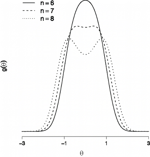
The difficulties in the study of the thermodynamic limit also apply to the study of the structural model g(θ). Since the structural model explicitly depends on p(x), it is clear that the problem of nonnested Curie-Weiss models also has implications for the structural model. To see that the scaling of σ is also important for the structural model, observe that it has one of two forms when μ_i = 0: it is unimodal when σ is sufficiently small and bimodal otherwise.⁴ Figure 8 shows this structural model for different values of n and a fixed value of σ, revealing that the value of σ for which g(θ) moves from a unimodal to a bimodal form depends on the value of n.⁵ When n grows indefinitely, the two modes tend to − ∞ and + ∞ for every fixed σ > 0, and consequently p(x) tends to have all probability mass on the ground states − 1_n and + 1_n. Thus, to observe nontrivial solutions for both p(x) and g(θ) in the limit n → ∞, the interaction strength σ needs to be a decreasing function of n.

Figure 8. The structural model g(θ) for in the absence of main effects, that is, μ_i = 0, and with an interaction strength σ = 0.075.

It is important to scale the interaction parameter σ with the right order and it turns out that a proper scaling⁶ is of order n: σ_n = σ/n. To see this, note first the following variant of Kac’s equality⁷: When applied to the Curie-Weiss model with interaction strength σ/n, this representation implies an M-RM with a scaled version of the structural model: a mixture of normal distributions g(θ∣x_n) with means and variances 2σ/n. Observe that for this posterior distribution both the means and variances are scaled by n and that the posterior distributions converge whenever each of the tend to a unique point Θ₀. This means that the latent variable is defined here as the limit of on an infinite network, and we implicitly assume that as n increases the intermediate networks form a sequence of models that become better approximations of this limiting network.

Before we proceed, some remarks are in order. First, we note that even though scaling the interaction strength by n provides interesting limiting behavior for both p(x_n) and g(θ∣x_n), it also implies a model that violates a fundamental principle in physics (Kac, 1968), as the interaction energy between two nodes i and j, − σ_nx_ix_j, now depends on the size of the system. Furthermore, in Figure 9 we illustrate that the structural model g_n(θ) that results from the derivation, has the property that it becomes more informative as n increases. Since the structural model g_n(θ) acts as a prior on the latent variable distribution (Marsman, Maris, Bechger, & Glas, 2016), we observe a prior distribution that becomes more informative as n increases. This may be a peculiar result to the Bayesian psychometrician.

Figure 9. The structural model g_n(θ) for in the absence of main effects, that is, μ_i = 0, and with a scaled interaction strength σ_n = σ/n = 0.45/n. We have used σ = 0.45 since then the scaled structural model for n = 6 variables shown here is identical to the structural model for n = 6 variables in Figure 8.

From Mark Kac to Mark Reckase

The theory that we have developed for the Curie-Weiss model carries over seamlessly to the more general Ising model. Let us first reiterate the Ising model: where we have used the interaction parameters σ_ij to encode the network structure. For instance, for the lattice in Figure 2 we have that σ_ij is equal to some constant σ if nodes i and j are direct neighbors on the lattice and that σ_ij is equal to zero when nodes i and j are no direct neighbors. Since we use the ± 1 notation for the spin random variables x_i, we observe that the terms σ_iix²_i = σ_ii cancel in the expression for the Ising model, as these terms are found in both the numerator and the denominator (something similar occurs in the “usual” notation).

We will use the eigenvalue decomposition of the so-called connectivity matrix to relate the Ising model to a multidimensional IRT model. However, since the elements σ_ii cancel in the expression of the Ising model, the diagonal elements of the connectivity matrix are undetermined. This indeterminacy implies that we have some degrees of freedom regarding the eigenvalue decomposition of the connectivity matrix. For now we will use: where Q is the matrix of eigenvectors, a diagonal matrix of eigenvalues and we have used to simplify the notation. The constant c serves to ensure that is a positive semi-definite matrix by translating the eigenvalues to be positive. Observe that this translation does not affect the eigenvectors but it does imply that only the relative eigenvalues—the eigen spectrum—are determined.

With the eigenvalue decomposition, we can write the Ising model in the convenient form: where we have used r to index the columns of A = [a_ir]. Applying Kac’s integral representation to each of the factors exp (∑_ia_irx_i)² reveals a multivariate latent variable expression for the Ising model, for which the latent variable model is known as the multidimensional two-parameter logistic model (MD-2PL; Reckase, 2009). The MD-2PL is closely related to the factor analytic model for discretized variables (Takane & de Leeuw, 1987), which is why we will refer to A as a matrix of factor-loadings. This formal connection between Ising network models and multidimensional IRT models proves the assertion of Molenaar (2003), who was the first to note this correspondence, and shows that to each Ising model we have a statistically equivalent IRT model.

New insight II: The identification problem of the multidimensional IRT model

The eigenvalue decomposition of

That the diagonal elements of the connectivity matrix are not identified certainly has implications for the interpretation of the latent variable model. The main observation is that there is no unique eigenvalue decomposition or matrix of loadings A that characterize a connectivity matrix. For instance, due to the indeterminacy of the diagonals of the connectivity matrix, we have that for every diagonal matrix C, the matrix characterizes the same marginal distribution p(x). That is, any such diagonal matrix does not alter the off-diagonal elements of the connectivity matrix, and thus the off-diagonal elements from are identified from the data. We assume here that the diagonal matrix ensures that the connectivity matrix is positive semi-definite, and use the eigenvalue decomposition: Although this decomposition retains the off-diagonal elements from the connectivity matrix, and thus A and A** characterize the same connectivity matrix (the diagonal elements are of no interest), it is in general unknown how A** relates to A.

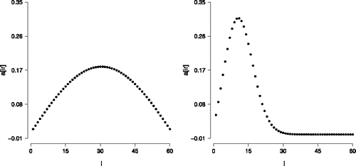
That the results can be strikingly different for different admissible choices for the diagonal elements of the connectivity matrix is illustrated in Figure 10, in which we show the first eigenvector that corresponds to the decomposition of a connectivity matrix using cI (left panel) and to a decomposition using a diagonal matrix C (right panel). Even though these eigenvectors, and the latent variable models that are characterized by them, are strikingly different, both characterize the same marginal distribution. Apart from the difficulty that this observation imposes on the interpretation of the multidimensional IRT model, it also suggests a problem with the identifiability of parameters in this IRT model. It is clear that a matrix of loadings holds little substance if it is not uniquely determined from the data, and one should be careful in interpreting the elements from such a matrix.

Figure 10. The first eigenvector corresponding to a decomposition of (left panel) and the first eigenvector corresponding to a decomposition of (right panel).

Nonidentification and the low-rank approximation to

That the matrix of loadings is not uniquely determined poses a practical problem for estimating the connectivity matrix using the latent variable representation, as we have suggested elsewhere (Marsman et al., 2015). First, there is no issue when we estimate a complete matrix of loadings since from this complete matrix of loadings we can construct the connectivity matrix. However, the connectivity matrix is typically large and consists of a substantial number of unknown parameters: n(n − 1)/2 to be precise. Using a well-known result from Eckart and Young (1936), who proved that the best rank R approximation to the full (connectivity) matrix is one where all but the R largest eigenvalues are equated to zero, we have suggested a low-rank approximation to the full-connectivity matrix. However, this low-rank approximation is not uniquely determined. We have used the diagonal matrix cI in our decomposition, which ensures that the largest estimated eigenvalues are also the largest eigenvalues of the complete connectivity matrix. However, the indeterminacy of the decomposition required us to consider the effect of choosing R on the connectivity matrix, not the estimated matrix of loadings. To this aim, we have used posterior predictive checks (Gelman, Meng, & Stern, 1996; Rubin, 1984), correlating the off-diagonal elements from the observed matrix of statistics that are sufficient for , that is, where p indexes the N observations, with the off-diagonal elements from the matrix of sufficient statistics computed on data generated using different ranks of approximation.

New insight III: Different mechanisms to generate correlations

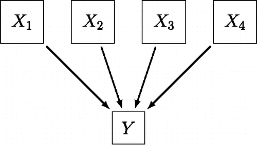
The common cause model, and the network or direct interaction model provide two distinct interpretations for the correlations that we observe in our data. In the common cause model it is assumed that the observed correlations are the result of an unobserved factor that is shared among observations, and in the network approach it is assumed that the observed correlations between variables are the result of their direct causal influences on each other. In theory, however, there may exist many such possible interpretations. A specific alternative, for instance, results from conceptualizing a theoretical construct as the direct effect of observables, known as a collider variable (Greenland, Pearl, & Robins, 1999; Pearl, 2000). Figure 11 shows such a common effect representation, in which the state of the observables X collectively cause the effect Y; for instance, observing major depression symptoms in a patient and the ensuing psychiatric evaluation of depression. Even though the observables may be marginally independent (Blalock, 1971; Bollen & Lennox, 1991), conditioning on the common effect results in associations between the observables (Elwert & Winship, 2014; Greenland et al., 1999; Greenland, 2003; Heckman, 1979; Hernán, Hernández-Diaz, & Robins, 2004). This provides us with a third possible interpretation; associations that arise through conditioning on a common effect.

Figure 11. A graphical representation of the common effect model. The observables X are the collective cause of the effect Y.

The formative model is probably the most widely known example of a model in which the observables X form causes of a (latent) common effect. For example, stressful life events such as getting divorced, changing jobs, or moving to a new home, are causes to the effect “exposure to stress” (Bollen & Lennox, 1991). The relation between the observables and the effect is usually of a linear nature, such that the higher a person scores on these observables, the more this person is exposed to stress. The formative model is typically used to predict the effect variable rather than to explain the relations between the causes.

We can use the aforementioned selection mechanism to form a third possible explanation for the relations among observables. Conditioning on the common effect in a collider model where the observables are marginally independent and each positively affects the common effect in a linear fashion, will result in negative associations between the observables. For example, given the information that a person has been diagnosed with depression but does have a particular symptom increases the probability that this person has any of the other depression symptoms. Observe that the relation between the observables and the effect does not need to be linear, and that there exist collider models that imply other structures for the associations among observables.

Recently, Kruis and Maris (2016) introduced the following collider model for the joint distribution of the observables X and their effect Y; where the effect can take on the values Y = 0 and Y = 1, and σ denotes the weight of Y on the X_i and is assumed to be equal for all observables. Kruis and Maris (2016) showed that the conditional distribution of observables X given the effect Y, that is, p(x∣Y = 1), is equivalent to the Curie-Weiss model. This connection can also be extended to the Ising model by replacing σx²₊ with the weighted sum (∑_ia_irx_i)², as we did before for the latent variable representation, and introducing an effect Y_r for every eigenvector. In this manner, the structure that is generated with an Ising model can also be generated with this collider model.

In contrast to a linear relation between causes and effect, the collider model that is proposed by Kruis and Maris (2016) suggests a quadratic relation. Since the observables take on the values x_i = −1 and x_i = +1, the model implies that when more observables are in the same state (either negative or positive) the probability of the effect being present increases if σ > 0, or decreases if σ < 0. It thus follows that conditioning on the effect being present (y = 1) implies that observables have a higher probability of being in the same state than in opposite states, thus inducing positive associations between the observables, given that σ > 0. When σ < 0, the opposite is implied: conditioning on the effect being present implies that variables have a higher probability to be in opposite states, thus inducing negative associations between the observables.

Causal versus statistical interpretations of the equivalent models

In evaluating the theoretical status of the presented model equivalence, it is important to make a distinction between the conceptual psychometric model (e.g., individual differences in a focal construct cause individual differences in the observed variables) and the statistical model typically associated with that conceptual model (e.g., the observations can be described by a common factor model). The reason that this distinction is important, is that several conceptual models can imply the same statistical model in a given data set. For example, behavior domains and reflective measurement models both can be represented by the latent variable model. In a behavior domain interpretation, the latent variable then corresponds to a tail measure defined on a behavior domain (roughly, a total score on an infinite set of items; Ellis & Junker, 1997). In a reflective interpretation, the latent variable corresponds to an unobserved common cause of the items, which screens off the empirical correlations between them (Pearl, 2000; Reichenbach, 1956). Because multiple conceptual models map to the same statistical model, the fit of a statistical model (i.e., a model that describes the joint probability distribution on a set of observables) does not license a definitive inference to a conceptual model (i.e., a model that describes the relation between observables and constructs), even though a conceptual model may unambiguously imply a particular statistical model.

For instance, in its original field of application, the model formulation in Equation (1(1) ) represents the physical interaction between particles. In this case, although the model utilizes statistical terminology to describe the relation between the particles, the model is not purely statistical, but also expresses causal information. For example, in the physical case, if the orientation of one of the particles were to be fixed by an external intervention, this would change the behavior of the neighboring particles as well; in particular, a manipulation that fixes the state of one of the particles would lead the remaining particles to form a new Ising model, for which the fixed particles would enter into the equation as part of the main effects (see Epskamp et al., in press, Equation (6)). Thus, in this case the model does not merely describe the statistical associations between a set of variables defined on the system, but also encodes the way in which the system would change upon manipulations of the system. As a result, in addition to representing statistical dependencies in a data set, in this case the edges connecting the nodes may also be interpreted as (giving rise to) bidirectional causal relations. The structure in Figure 2 then encodes a graphical causal model (Pearl, 2000), which could be conceptually fleshed out in terms of an interventionist framework, where by X counts as a cause of Y if an intervention on X were to change the probability distribution of Y (Woodward, 2003).

It is important to note that this causal interpretation is not mandated by the probabilistic structure represented in Equation (1(1) ) in itself. Statistically speaking, the model is merely a convenient representation of a probability distribution that is described by a loglinear homogenous association model (i.e., a loglinear model with an intercept and pairwise interaction terms, but without higher order interactions; Wickens, 1989). This loglinear model in itself does not carry any causal information, because it does not mandate how the system will change upon manipulation of its constituent variables. Thus, to get to the implication of how the system would behave under a given intervention that fixes the state of a given variable in the model, the statistical model has to be augmented by causal assumptions (Pearl, 2000). These causal assumptions require theoretical motivation. In the classical application of the Ising model in physics, this motivation is given by the general theory of magnetism. In the case of the psychopathology example in Figure 3, they could be motivated by, for example, observations of patients, general knowledge of the human system, or research that involves interventions on individual symptoms.

Finally, it is useful to point out the asymmetry in moving from the conceptual model to the statistical model versus moving in the other direction. A theoretical model can have definite implications for the type of statistical model that one expects to hold for the observations. For instance, if one believes that correlated individual differences in cognitive test scores are due to the common influence of general intelligence or mental energy, as Spearman (1904) did, this motivates the expectation that a common factor model will fit the data. However, this motivation is not unique to the common cause model. If another researcher believes that individual differences in cognitive test scores are correlated, because they sample the same cognitive processes, as Thomson (1916) did, this can (and does) also lead to the expectation that a common factor model will describe the data. Finally, it has been shown that the mutualism model of van der Maas et al. (2006), in which cognitive tests measure attributes that reinforce each other during development, also implies the fit of a common factor model. Because each of these models implies the same probability distribution for the data, one cannot conclude from the fit of the statistical model that the conceptual model is accurate.

Thus, causal interpretations do not follow from the statistical model alone, as indeed they never do. In addition, the mapping from statistical association structure to a generating causal structure is typically one-to-many, which means that many different underlying causal models can generate the same set of statistical relations. This fact blocks direct inference from the statistical model to the causal model, a problem known to SEM researchers as the problem of equivalent models (Markus, 2002), to philosophers as (one of the incarnations of) the problem of induction (Hume, 1896), and to the general audience as the platitude “correlation does not imply causality.” However, given a set of equivalent conceptual models, it is often possible to disentangle which one is most accurate by extending one’s set of measurements, or through experimental interventions for which the models imply divergent predictions.

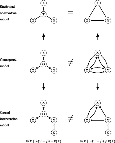
Figure 12 suggests some ways in which this may happen. We start with two different conceptual models (represented in the middle panel). For instance, one researcher may posit a reflective latent variable model, which specifies correlations between observables to arise from the pervasive influence of a common cause, while another researcher may hold that these correlations arise from reciprocal causal relations in a fully connected network structure. In this case, both researchers would expect the same probability distribution to describe the data, which can be either represented as an IRT model using a latent variable, or as a fully connected network of conditional associations; this is the equivalence we have exploited in the current paper. Yet, if the possibility to intervene causally arises, it is still possible to disentangle the conceptual models: for an intervention in one indicator variable (which can be represented using Pearl’s do-operator; Pearl, 2000) will change the probability distribution of other indicator variables in a network model, but not in a common cause model. Thus, the equivalence shown here is not a full-blown equivalence of theoretical models, but only of statistical models that describe a given data set. Importantly, however, this does mean that causal interventions will have to play a central role in research that tries to distinguish common cause explanations from network explanations of correlation patterns in the data. Of course, this only works if one has a fully reflective latent variable model as one’s conceptual model, in which there is no feedback between the indicator variables and the latent variable; as soon as such feedback is allowed, the current setup would not allow one to distinguish the conceptual models.

Figure 12. The relation between conceptual, statistical, and causal models. Two different conceptual models (middle panel) that imply the same statistical observation model (top panel) can often still be teased apart using causal interventions (bottom panel).

It is important to observe that statistical equivalence can never be fully eradicated. Even when we have a causal intervention, that will by necessity result in a data set that again has two possible statistically equivalent descriptions, using either a multidimensional IRT model or an Ising model. Rather than weeding out statistical equivalence in general, causal interventions thus allow one to distinguish between particular sets of conceptual models.

Network psychometrics in practice

Figure 7 illustrates that the latent variable distribution g(θ) that is used in the M-RM representation of the Curie-Weiss model can generate different shapes. Most importantly, the latent variable distribution resembles a normal distribution when the interaction strength σ is sufficiently low (or equivalently that the temperature τ is sufficiently high, see footnote 4). This suggests that an M-RM with the typically used normal latent variable model f(θ) will fit to data that comes from a Curie-Weiss model with a sufficiently low interaction strength σ, but it will not fit when σ is too high. In this case the latent variable distribution g(θ) that is used in the M-RM representation of the Curie-Weiss model becomes either skewed or bimodal, see, Figure 7. We provide two illustrations of the practical application of the M-RM to data that comes from a Curie-Weiss network. The first illustration confirms our intuition that the M-RM with the typically used normal latent variable model f(θ) will fit to data that is generated from a Curie-Weiss model when the interaction strength is sufficiently low, but not when the interaction strength is too high. The second illustration demonstrates that for cases where σ is too high the fit of the M-RM can be significantly improved when a finite mixture of normal distributions is used as latent variable model f(θ) instead of the usual normal distribution (Marsman et al., 2012). Specifically, with a mixture of two normal distributions we are able to generate the bimodal and skew latent variable distributions that are observed when σ is high.

A serious complication in the evaluation of the latent variable model f(θ) is that the latent variables are not observed. To overcome this complication, we may replace each of the nonobserved latent variables θ with a plausible value θ* (Mislevy, 1991, 1993; Mislevy, Beaton, Kaplan, & Sheehan, 1992). A plausible value for a person p with an observed configuration of scores x_p is a random draw from his or her posterior distribution f(θ∣x_p). Observe that replacing the nonobserved latent variables with plausible values is much like imputing missing data points (Rubin, 1987). The plausible values are used to infer about the fit of the latent variable model f(θ) by comparing their empirical CDF with the CDF of the latent variable model using the Kolmogorov–Smirnov (KS) test (e.g., Berger & Zhou, 2014). The reason that we use plausible values to evaluate the fit of the latent variable model f(θ) is two-fold. First, the true latent variable distribution g(θ) is not known in practice, and plausible values offer a practical alternative since they can be analyzed as if the latent variables were observed. Second, we have shown that the marginal distribution of plausible values is the best estimator of the true—but unknown—latent variable distribution (Marsman et al., 2016). Specifically, our results imply that the marginal distribution of plausible values will be closer⁸ to the true—but unknown—latent variable distribution than the latent variable model f(θ), except when the latent variable model f(θ) and the true latent variable distribution g(θ) are the same. One way to interpret this result is that the model f(θ)—the normal distribution—acts like a prior on the distribution of latent variables, and that the observed data are used to update this prior to a posterior distribution of the latent variables; the distribution of plausible values.

Illustration I: The M-RM with a normal latent variable model f(θ)

In the first illustration, we will use a Normal distribution for the latent variables in the M-RM. We fix the item difficulty parameters of the Rasch model to the Curie-Weiss model’s main effects (i.e., δ_i = −μ_i), and focus on evaluating the fit of the normal latent variable model. The unknown parameters λ and φ need to be estimated from the data. We will use a Bayesian approach to estimate both the unknown model parameters and the latent variables. To this aim, we need to specify a prior distribution for the two unknown parameters, and here we will use Jeffreys’s prior (Jeffreys, 1961). The advantage of this prior distribution is that it is relatively noninformative. With the prior distribution specified, we can invoke Bayes’ rule to formulate the joint posterior distribution where the latent variable model is the Normal distribution, the conditional distribution of the observed data is the Rasch model, and X denotes the matrix of observations. In our analyses, we generate N = 10, 000 cases from an n = 20 variable Curie-Weiss network, such that X is of dimension N by n. Observe that the joint posterior distribution is not available in closed form, but we can make use of the Gibbs sampler to simulate from it (Geman & Geman, 1984; Gelfand & Smith, 1990).

Simulating from the joint posterior distribution using the Gibbs sampler boils down to simulating from three distinct full-conditional distributions. The first full-conditional distribution is the posterior distribution of the population mean , which is equal to a Normal distribution. The second full-conditional distribution is the posterior distribution of the population standard deviation , and we find that the precision φ^{− 2} a posteriori follows a Gamma distribution. The final full-conditional distribution is that of the latent variables , which conveniently factors in N independent posterior distributions , for p = 1, …, N. These posterior distributions are not available in closed form, but Marsman, Maris, Bechger, and Glas (2017) recently proposed an independence chain Metropolis approach (Tierney, 1994, 1998) that is based on the Exchange algorithm of Murray, Ghahramani, and MacKay (2006) to efficiently simulate from .^{Figure 13}

We generated 25 data sets each for a range of interaction strengths σ. For each data set, we apply our M-RM and estimate the model’s parameters and latent variables using the Gibbs sampler. In each case, we ran the Gibbs sampler for 500 iterations. The average acceptance rate of our independence Metropolis approach to simulate from the posteriors of the latent variables was approximately 94%, which ensured that convergence of the Markov chain was almost immediate. Observe that the plausible values are a by-product of our Gibbs sampler, that is, they are the draws from the full-conditional posterior distribution . We compute P-values from the KS-tests⁹ applied to the plausible values that were generated every 50th iteration of the Gibbs sampler, so that for every value of σ we obtain the P-values from 10 repetitions for each of the 25 data sets.

The results are shown in the left panel of Figure 13, where we plot the average P-value against the interaction strength σ. Observe that for σ values that are smaller than approximately 0.027 the P-values average to approximately 0.5, the expected P-value under . At about the value σ = 0.033 the KS-test is significant at an α-level of 0.05, which indicates that the plausible value distribution and the normal latent variable model have diverged. To gauge the severity of this mismatch, we show the true latent variable distribution g(θ) (gray solid line), our normal latent variable model f(θ) (black solid line) and the empirical CDF of plausible values (black dotted line) in the right panel of Figure 13 for σ = 0.04. Observe that the distribution of plausible values is able to reproduce the bimodal shape of g(θ), where the normal latent variable model f(θ) cannot reproduce this shape. However, we can also observe clear differences between the distribution of plausible values and the true latent variable distribution. The primary reason for this difference is that the normal latent variable model still has a strong influence on the distribution of plausible values. However, convergence of the distribution of plausible values to the true latent variable distribution g(θ) might be improved by using a more flexible prior latent variable model f(θ) (Marsman et al., 2016), such as a mixture of normal distributions.

Figure 13. The left panel shows the average P-value obtained from KS-tests comparing the empirical CDF of plausible value with the Normal CDF for different values of the interaction strength σ. The right panel shows the true CDF of the latent variables (gray solid line), the estimated Normal CDF (black solid line), and the empirical CDF of plausible values (black dotted line) for σ = 0.04.

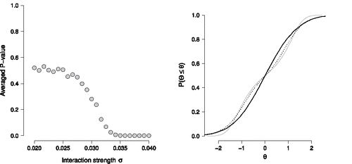
Illustration II: The M-RM with a mixture latent variable model f(θ)

To accommodate for a bimodal or skewed distribution of latent variables, we proposed to use a discrete mixture of normal distributions as a latent variable model in the M-RM (Marsman et al., 2012). Specifically, we have used the two component mixture of normals, where denotes the normal density with mean λ_i and variance φ²_i, and showed that this mixture can generate bimodal and skewed latent variable distributions. The mixture distribution may be interpreted as follows. Suppose that you flip a coin z that lands heads (z = 1) with probability equal to γ and lands tails (z = 0) with probability 1 − γ. We generate the latent variable θ from a Normal distribution if the coin lands heads, and generate the latent variable from a Normal distribution if the coin lands tails. This interpretation suggests an augmented variable approach to analyze the discrete mixture model: Introduce a binary augmented variable z that allocates cases to one of the two mixture components, such that (6) We will use this two-component mixture as latent variable model f(θ).^{Figure 14}

We will again use a Bayesian approach to estimate the unknown parameters of the latent variable model f(θ) and the latent variables. As before, we will use Jeffreys’s approach to specify a noninformative prior for the unknown population parameters This leads to the following joint posterior distribution: where the conditional distribution is the distribution in (6(6) ), and p(z∣γ) is a Bernoulli(γ) distribution. Simulating from the joint posterior distribution using the Gibbs sampler boils down to simulating from the following five full-conditional^{Figure 14}distributions:

(1)	The full-conditionals of the N binary allocation variables are Bernoulli distributions with success probabilities: for p = 1, …, N.
(2)	The full-conditionals of the latent variables are of the same form as before, except that the “prior” on θ is the Normal distribution for cases where zp = 1 and the Normal distribution for cases where zp = 0.
(3)	The full-conditionals of the two population means λ1 and λ2 are normal distributions. Specifically, the full-conditional of λ1 is a Normal, where is the mean of the n1 cases for which z = 1 (i.e., n1 = ∑pzp). Similarly, the full-conditional of λ2 is a Normal, where is the mean of the n2 cases for which z = 0 (i.e., n2 = ∑p(1 − zp) = N − n1).
(4)	The full-conditionals of the two precision parameters φ− 21 and φ− 22 are gamma distributions. Specifically, the full-conditional of φ− 21 is a Gamma distribution, and the full-conditional distribution of φ− 22 is a Gamma distribution.
(5)	The full-conditional of the mixture probability γ is a Beta distribution.

Thus, each of the full-conditional distributions is readily sampled from.

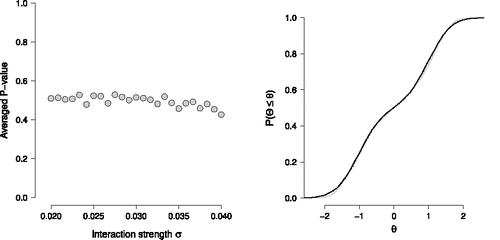
The results of our analysis with the mixture model are shown in the left panel of Figure 14. Observe that the P-values¹⁰ now average to approximately 0.5 across the entire range of interaction strengths σ, which indicate that the plausible values and the mixture model did not diverge. The true latent variable distribution g(θ) (gray solid line), our mixture latent variable model f(θ) (black solid line) and the empirical CDF of plausible values (back dotted line) are shown in the right panel of Figure 14 for σ = 0.04. Observe that both the mixture distribution f(θ) and the plausible value distribution now closely resemble the true latent variable distribution g(θ).

Figure 14. The left panel shows the average P-value obtained from KS-tests comparing the empirical CDF of plausible value with the estimated Normal mixture CDF for different values of the interaction strength σ. The right panel shows the true CDF of the latent variables (gray solid line), the estimated Normal mixture CDF (black solid line), and the empirical CDF of plausible values (black dotted line) for σ = 0.04.

We conclude that even though the data come from a statistical model that is associated with a wildly distinct conceptual framework, the M-RM that is associated to a common cause interpretation fits the data remarkably well in practice. Especially the use of a mixture of two normal distributions as a latent variable model provides a good fit of the M-RM to network data, and with only three additional parameters this is a small price to pay. These results imply that many of the methods that have been designed to analyze binary data using marginal IRT models are also useful to analyze binary data from a network perspective, and vice versa. That is, the statistical equivalence might not only bring new theoretical insights but also provide practical benefits. For instance, we may use IRT models to handle missing observations in applications of network models (Marsman, Waldorp, & Maris, 2016), or may use network models to reveal the residual structure in an IRT analysis (Chen, Li, Liu, & Ying, 2016; Epskamp, Rhemtulla, & Borsboom, 2017).

Discussion

The current paper has explored connections between the worlds of statistical physics and psychometrics. By establishing the equivalence of two canonical models from these fields—the Lenz-Ising model and the IRT model—a systematic connection has been forged that allows us to cross-fertilize each of the fields with representations, techniques, and insights from the other. In particular, we think that psychometrics stands to gain from this connection, because the network modeling framework yields a theoretically plausible modeling approach for dealing with classic psychometric questions.

We have shown that Kac’s Gaussian integral representation can be used to relate the network models of Lenz and Ising to the latent variable models of Rasch and Reckase. Specifically, the models were seen to correspond to a different factorization of the joint distribution of the manifest and latent variables: where the latter factorization also revealed the graphical models that were originally proposed by Olkin & Tate, and later popularized by Lauritzen & Wermuth. We have investigated some of the implications of these relations to the existing psychometric theory.

That the network models of Lenz and Ising directly relate to the IRT models of Rasch and Reckase implies that every observed association (of binary random variables) can be given two interpretations: The associations can be interpreted to arise from a direct influence between variables or due to an underlying and unobserved (set of) common cause(s). Additionally, we have shown that the recent work of Kruis and Maris (2016) provides yet a third possible interpretation; an observed association that results from conditioning on a common effect. In fact, there might be many possible ways to interpret an observed association, and the fit of a statistical model does not guarantee that we have chosen the right one. This urges us to be cautious with our interpretations, especially since this may have a strong influence on the type of questions that we ask (i.e., the research that we perform) or, more importantly, the type of questions that we do not ask. For instance, questions about measurement invariance and correlational structure may be interesting from a common cause approach but not from a network approach, whereas researchers that take a network approach are more likely to ask questions about the dynamical aspects of a system, such as hysteresis and critical slowing down. The observed statistical equivalences make it easier to switch between the conceptual approaches, such that we can study different aspects of our substantive theories. Ultimately, this will further our understanding about the many distinct psychological constructs that have been formulated, and how they relate to observable behaviors.

It is also important, then, to investigate how the network of statistical models in Figure 1 expands to include other models. Several relations to statistical models displayed in Figure 1 can be observed in the psychometric-, econometric-, statistics-, and physics-literature. For instance, relations between the item response theory models in Figure 1 and other latent variable models have been described by Takane and de Leeuw (1987) and Thissen and Steinberg (1986), but see also the work of Kamata and Bauer (2008) and Bartolucci and Pennoni (2007), for instance. Furthermore, these IRT models were also studied in relation to models that originate from mathematical psychology by Tuerlinckx and de Boeck (2005) and van der Maas, Molenaar, Maris, Kievit, and Borsboom (2011). Similarly, we observe in the physics literature that the Ising network model is a special case of the Potts network model (Ashkin & Teller, 1943; Potts, 1952), Markov random fields (Kindermann & Snell, 1980), and it has also been related to the percolation theory of Broadbent and Hammersley (1957) through the work of Fortuin and Kasteleyn (1972). Finally, we observe that the work described in Hessen (2012) provides an interesting extension to models for categorical random variables. Without trying to produce an exhaustive list of relations to the models considered in this article, we hope that it is clear that the network of statistical models displayed in Figure 1 is a small subset of a formidable network of statistical models. What is not clear, however, is how these statistical models that originate from distinct scientific fields relate to one another, but the relations that have been discussed in this paper form an important first step to answer this question.

Article Information

Conflict of Interest Disclosures: Each author signed a form for disclosure of potential conflicts of interest. No authors reported any financial or other conflicts of interest in relation to the work described.

Ethical Principles: The authors affirm having followed professional ethical guidelines in preparing this work. These guidelines include obtaining informed consent from human participants, maintaining ethical treatment and respect for the rights of human or animal participants, and ensuring the privacy of participants and their data, such as ensuring that individual participants cannot be identified in reported results or from publicly available original or archival data.

Role of the Funders/Sponsors: None of the funders or sponsors of this research had any role in the design and conduct of the study; collection, management, analysis, and interpretation of data; preparation, review, or approval of the manuscript; or decision to submit the manuscript for publication.

Acknowledgments: The ideas and opinions expressed herein are those of the authors alone, and endorsement by the authors' institutions or the funding agencies is not intended and should not be inferred.

Additional information

Funding

This work was supported by Grants 314-99-107, 406-11-066, and 022.005.0 from the Netherlands Organisation for Scientific Research (NWO), and Grant 647209 from the European Research Council (ERC).

Notes

1 In statistics, it is common practice to code binary variables as . We will use the ± 1 coding for historical purposes and because it makes some of the mathematics particularly simple.

2 Note that we have used the ± 1 coding to express the Rasch model, which is slightly different than the usual expression for binary variables : This difference is only cosmetic as one can simply traverse between the two notational schemes.

3 That the Curie-Weiss model is a marginal Rasch model and was proposed in the physics literature far before the Rasch model was introduced in the psychometric literature, gives a counter-example to the maxim of Andrew Gelman: “whatever you do, somebody in psychometrics already did it long before” (see http://andrewgelman.com/2009/01/26/a_longstanding/). In fact, the Rasch model itself was already proposed by the physicist and logician Zermelo back in 1929 (see also Zermelo, 2001).

4 In physics, the value σ is related to the inverse temperature, say (Kac, 1968): where τ refers to temperature, κ to a constant value (Boltzman’s constant), and λ to the scaled interaction effect. The point τ_C at which g(θ) changes between the unimodal and bimodal form is known as the critical temperature.

5 See van der Maas, Kan, Marsman, and Stevenson (2017) for the conceptual implications of this property in the context of cognitive development and intelligence.

6 Note that there are possibly other scaling factors for which the posterior distributions converge. For instance, σ_n = o(nlog n). However, we have already seen that the constant σ_n = o(1) provides a trivial solution. It can also be seen that for the quadratic σ_n = o(n^{− 2}) all posterior distribution converge to the prior mean and the marginal p(x) becomes a uniform distribution over the possible configurations x.

7 We have used the change of variable θ = 2 σ_n θ*.

8 In expected Kullback–Leibler divergence.

9 The KS-test is a nonparametric test for the equality of two (continuous) one-dimensional probability distributions, which can be used to compare an empirical CDF against a reference distribution (e.g., Berger & Zhou, 2014). Here, we compare the empirical CDF of plausible values against the estimated Normal CDF (i.e., the reference distribution). The associated null-hypothesis stipulates that the empirical CDF of plausible values coincides with the estimated Normal CDF.

10 Using the estimated mixture of Normal CDFs as reference distribution in the KS-test.

References

- Adams, R., Wilson, M., & Wu, M. (1997). Multilevel item response models: An approach to errors in variables regression. Journal of Educational and Behavioral Statistics, 22(1), 47–76. doi: 10.3102/10769986022001047
- Anderson, C., Li, Z., & Vermunt, J. (2007). Estimation of models in a Rasch family of polytomous items and multiple latent variables. Journal of Statistical Software, 20(6), 1–36. doi: 10.18637/jss.v020.i06
- Anderson, C., & Vermunt, J. (2000). Log-multiplicative association models as latent variable models for nominal and/or ordinal data. Sociological Methodology, 30(1), 81–121. doi: 10.1111/0081-1750.00076
- Anderson, C., & Yu, H. (2007). Log-multiplicative association models as item response models. Psychometrika, 72(1), 5–23. doi: 10.1007/s11336-005-1419-2
- Ashkin, J., & Teller, E. (1943). Statistics of two-dimensional lattices with four components. Physical Review, 64(5–6), 178–184. doi: 10.1103/PhysRev.64.178
- Bartolucci, F., & Pennoni, F. (2007). On the approximation of the quadratic exponential distribution in a latent variable context. Biometrika, 94(3), 745–754. doi: 10.1093/biomet/asm045
- Bechger, T., & Maris, G. (2015). A statistical test for differential item pair functioning. Psychometrika, 80(2), 317–340. doi: 10.1007/s11336-014-9408-y
- Berger, V., & Zhou, Y. (2014). Kolmogorov–Smirnov test: Overview. In Wiley statsref: Statistics reference online. New York: John Wiley & Sons, Ltd. doi: 10.1002/9781118445112.stat06558
- Birnbaum, A. (1968). Some latent trait models and their use in inferring an examinee’s ability. In F. M. Lord & M. R. Novick (Eds.), Statistical theories of mental test scores (pp. 395–479). Reading: Addison-Wesley.
- Blalock, H. (1971). Causal models involving unmeasured variables in stimulus response situations. In H. Blalock (Ed.), Causal models in the social sciences (pp. 335–347). Chicago: Aldine-Atherton.
- Bock, R., & Aitken, M. (1981). Marginal maximum likelihood estimation of item parameters: Application of an EM algorithm. Psychometrika, 46(4), 179–197. doi: 10.1007/BF02293801
- Bollen, K., & Lennox, R. (1991). Conventional wisdom on measurement: A structural equation perspective. Psychological Bulletin, 110(2), 305–314. doi: 10.1037/0033-2909.110.2.305
- Borsboom, D. (2008). Psychometric perspectives on diagnostic systems. Journal of Clinical Psychology, 64(9), 1089–1108. doi: 10.1002/jclp.20503
- Borsboom, D., & Cramer, A. (2013). Network analysis: An integrative approach to the structure of psychopathology. Annual Review of Clinical Psychology, 9, 91–121. doi: 10.1146/annurev-clinpsy-050212-185608
- Borsboom, D., & Molenaar, D. (2015). Psychometrics. In J. Wright (Ed.), International encyclopedia of the social & behavioral sciences ( Second ed., Vol. 19, pp. 418–422). Amsterdam: Elsevier.
- Brennan, R. L. (2001). Generalizability theory. New York: Springer-Verlag.
- Broadbent, S., & Hammersley, J. (1957). Percolation processes: I. Crystals and mazes. Proceedings of the Cambridge Philosophical Society, 53(3), 629–641. doi: 10.1017/S0305004100032680
- Brout, R. (1968). Phase transitions. In M. Chrétien, E. Gross, & S. Deser (Eds.), Statistical physics: Phase transitions and superfluidity, vol. 1, Brandeis university summer institute in theoretical physics (pp. 1–100). New York: Gordon and Breach Science Publishers.
- Brush, S. (1967). History of the Lenz-Ising model. Reviews of Modern Physics, 39(4), 883–895. doi: 10.1103/RevModPhys.39.883
- Chang, H.-H. (1996). The asymptotic posterior normality of the latent trait for polytomous IRT models. Psychometrika, 61(3), 445–463. doi: 10.1007/BF02294549
- Chang, H.-H., & Stout, W. (1993). The asymptotic posterior normality of the latent trait in an IRT model. Psychometrika, 58(1), 37–52. doi: 10.1007/BF02294469
- Chen, Y., Li, X., Liu, J., & Ying, Z. (2016). A fused latent and graphical model for multivariate binary data. arXiv preprint arXiv:1606.08925.
- Cox, D. (1972). The analysis of multivariate binary data. Journal of the Royal Statistical Society. Series C (Applied Statistics), 21(2), 113–120. doi: 10.2307/2346482
- Cox, D., & Wermuth, N. (2002). On some models for multivariate binary variables parallel in complexity with the multivariate Gaussian distribution. Biometrika, 89(2), 462–469. doi: 10.1093/biomet/89.2.462
- Cramer, A., Waldorp, L., van der Maas, H., & Borsboom, D. (2010). Comorbidity: A network perspective. Behavioral and Brain Sciences, 33(2–3), 137–150. doi: 10.1017/S0140525X09991567
- Cressie, N., & Holland, P. (1983). Characterizing the manifest probabilities of latent variable models. Psychometrika, 48(1), 129–141. doi: 10.1007/BF02314681
- Cronbach, L., Gleser, G., Harinder, N., & Rajaratnam, N. (1972). The dependability of behavioral measurements: Theory of generalizability for scores and profiles. New York: John Wiley & Sons.
- Cronbach, L., & Meehl, P. (1955). Construct validity on psychological tests. Psychological Bulletin, 52(4), 281–302. doi: 10.1037/h0040957
- Cronbach, L., Rajaratnam, N., & Gleser, G. (1963). Theory of generalizability: A liberation of reliability theory. British Journal of Mathematical and Statistical Psychology, 16(2), 137–163. doi: 10.1111/j.2044-8317.1963.tb00206.x
- de Leeuw, J., & Verhelst, N. (1986). Maximum likelihood estimation in generalized Rasch models. Journal of educational statistics, 11(3), 183–196. doi: 10.2307/1165071
- Eckart, C., & Young, G. (1936). The approximation of one matrix by another of lower rank. Psychometrika, 1(3), 211–218. doi: 10.1007/BF02288367
- Edwards, J., & Bagozzi, R. (2000). On the nature and direction of relationships between constructs and measures. Psychological Methods, 5(2), 155–174. doi: 10.1037/1082-989X.5.2.155
- Ellis, J., & Junker, B. (1997). Tail-measurability in monotone latent variable models. Psychometrika, 62(4), 495–523. doi: 10.1007/BF02294640
- Elwert, F., & Winship, C. (2014). Endogenous selection bias: The problem of conditioning on a collider variable. Annual Review of Sociology, 40, 31–53. doi: 10.1146/annurev-soc-071913-043455
- Embretson, S., & Reise, S. (2000). Item response theory for psychologists. London: Lawrence Erlbaum Associates.
- Emch, G., & Knops, H. (1970). Pure thermodynamical phases as extremal KMS states. Journal of Mathematical Physics, 11, 3008–3018. doi: 10.1063/1.1665087
- Epskamp, S., Maris, G., Waldorp, L., & Borsboom, D. (in press). Network psychometrics. In P. Irwing, D. Hughes, & T. Booth (Eds.), Handbook of psychometrics. New York: Wiley.
- Epskamp, S., Rhemtulla, M., & Borsboom, D. (2017). Generalized network psychometrics: Combining network and latent variable models. Psychometrika [in press]. doi: 10.1007/s11336-017-9557-x
- Fierst, J., & Phillips, P. (2015). Modeling the evolution of complex genetic systems: The gene network family tree. Journal of Experimental Zoology Part B: Molecular and Developmental Evolution, 324(1), 1–12. doi: 10.1002/jez.b.22597
- Fortuin, C., & Kasteleyn, P. (1972). On the random-cluster model: I. Introduction and relation to other models. Physica, 57(4), 536–564. doi: 10.1016/0031-8914(72)90045-6
- Galam, S., Gefen, Y., & Shapir, Y. (1982). Sociophysics: a new approach of sociological collective behavior. Journal of Mathematical Sociology, 9(1), 1–13. doi: 10.1080/0022250X.1982.9989929
- Galam, S., & Moscovici, S. (1991). Towards a theory of collective phenomena: Consensus and attitude changes in groups. European Journal of Social Psychology, 21(1), 49–74. doi: 10.1002/ejsp.2420210105
- Gelfand, A., & Smith, A. (1990). Sampling-based approaches to calculating marginal densities. Journal of the American Statistical Association, 85(410), 398–409. doi: 10.2307/2289776
- Gelman, A., Meng, X., & Stern, H. (1996). Posterior predictive assessment of model fitness via realized discrepancies. Statistica Sinica, 6(4), 733–760.
- Geman, S., & Geman, D. (1984). Stochastic relaxation, Gibbs distributions, and the Bayesian restoration of images. IEEE Transactions on Pattern Analysis and Machine Intelligence, 6(6), 721–741. doi: 10.1109/TPAMI.1984.4767596
- Glas, C. (1989). Contributions to estimating and testing Rasch models ( Unpublished doctoral dissertation). University of Twente, Enschede, Netherlands.
- Greenland, S. (2003). Quantifying biases in causal models: Classical confounding vs collider-stratification bias. Epidemiology, 14(3), 300–306. doi: 10.1097/01.EDE.0000042804.12056.6C
- Greenland, S., Pearl, J., & Robins, J. (1999). Causal diagrams for epidemiological research. Epidemiology, 10(1), 37–48.
- Heckman, J. (1979). Sample selection bias as a specification error. Econometrica, 47(1), 153–161. doi: 10.2307/1912352
- Hernán, M., Hernández-Diaz, S., & Robins, J. (2004). A structural approach to selection bias. Epidemiology, 15(5), 615–625. doi: 10.1097/01.ede.0000135174.63482.43
- Hessen, D. (2011). Loglinear representations of multivariate Bernoulli Rasch models. British Journal of Mathematical and Statistical Psychology, 64(2), 337–354. doi: 10.1348/2044-8317.002000
- Hessen, D. (2012). Fitting and testing conditional multinormal partial credit models. Psychometrika, 77(4), 693–709. doi: 10.1007/s11336-012-9277-1
- Holland, P. (1990). The Dutch identity: A new tool for the study of item response models. Psychometrika, 55(6), 5–18. doi: 10.1007/BF02294739
- Hume, D. (1896). A treatise of human nature. Oxford, UK: Clarendon Press.
- Ising, E. (1925). Beitrag zur theorie des ferromagnetismus. Zeitschrift für Physik, 31(1), 253–258. doi: 10.1007/BF02980577
- Jeffreys, H. (1961). Theory of probability (third ed.). Oxford, UK: Oxford University Press.
- Kac, M. (1968). Mathematical mechanisms of phase transitions. In M. Chrétien, E. Gross, & S. Deser (Eds.), Statistical physics: Phase transitions and superfluidity, vol. 1, Brandeis university summer institute in theoretical physics (pp. 241–305). New York: Gordon and Breach Science Publishers.
- Kamata, A., & Bauer, D. (2008). A note on the relation between factor analytic and item response theory models. Structural Equation Modeling, 15(1), 136–153. doi: 10.1080/10705510701758406
- Kindermann, R., & Snell, J. (1980). Markov random fields and their applications (Vol. 1). Providence, Rhode Island: American Mathematical Society.
- Kochmański, M., Paskiewicz, T., & Wolski, S. (2013). Curie-Weiss magnet–a simple model of phase transition. European Journal of Physics, 34(6), 1555–1573.
- Kruis, J., & Maris, G. (2016). Three representations of the Ising model. Scientific Reports, 6(34175), 1–11. doi: 10.1038/srep34175
- Lauritzen, S. (1996). Graphical models. Oxford: Oxford University Press.
- Lauritzen, S., & Wermuth, N. (1989). Graphical models for associations between variables, some of which are qualitative and some quantitative. The Annals of Statistics, 17(1), 31–57. doi: 10.1214/aos/1176347003
- Lenz, W. (1920). Beiträge zum verständnis der magnetischen eigenschaften in festen körpern. Physikalische Zeitschrift, 21, 613–615.
- Maris, G., Bechger, T., & San Martin, E. (2015). A Gibbs sampler for the (extended) marginal Rasch model. Psychometrika, 80(4), 859–879. doi: 10.1007/s11336-015-9479-4
- Markus, K. (2002). Statistical equivalence, semantic equivalence, eliminative induction, and the Raykov-Marcoulides proof of infinite equivalence. Structural Equation Modeling, 9(4), 503–522. doi: 10.1207/S15328007SEM0904_3
- Markus, K., & Borsboom, D. (2013). Frontiers of test validity theory: Measurement, causation, and meaning. New York, NY: Routledge.
- Marsman, M., Maris, G., & Bechger, T. (2012). Don’t tie yourself to an onion: Don’t tie yourself to assumptions of normality. In T. Eggen & B. Veldkamp (Eds.), Psychometrics in practice at RCEC (pp. 103–114). Enschede: RCEC.
- Marsman, M., Maris, G., Bechger, T., & Glas, C. (2015). Bayesian inference for low-rank Ising networks. Scientific Reports, 5(9050), 1–7. doi: 10.1038/srep09050
- Marsman, M., Maris, G., Bechger, T., & Glas, C. (2016). What can we learn from Plausible Values? Psychometrika, 81(2), 274–289. doi: 10.1007/s11336-016-9497-x
- Marsman, M., Maris, G., Bechger, T., & Glas, C. (2017). Turning simulation into estimation: Generalized exchange algorithms for exponential family models. PLoS One, 12(1), e0169787. doi: 10.1371/journal.pone.0169787
- Marsman, M., Waldorp, L., & Maris, G. (2016). A note on large-scale logistic prediction: Using an approximate graphical model to deal with collinearity and missing data. [in press]. doi: 10.1007/s41237-017-0024-x
- McCullagh, P. (1994). Exponential mixtures and quadratic exponential families. Biometrika, 81(4), 721–729. doi: 10.2307/2337075
- McDonald, R. P. (2003). Behavior domains in theory and in practice. The Alberta Journal of Educational Research, 49(3), 212–230.
- Mellenbergh, G. (1994). Generalized item response theory. Psychological Bulletin, 115(2), 300–307. doi: 10.1037/0033-2909.115.2.300
- Mislevy, R. (1991). Randomization-based inference about latent variables from complex samples. Psychometrika, 56(2), 177–196. doi: 10.1007/BF02294457
- Mislevy, R. (1993). Should “multiple imputations” be treated as “multiple indicators”? Psychometrika, 58(1), 79–85. doi: 10.1007/BF02294472
- Mislevy, R., Beaton, A., Kaplan, B., & Sheehan, K. (1992). Estimating population characteristics from sparse matrix samples of item responses. Journal of Educational Measurement, 29(2), 133–161. doi: 10.1111/j.1745-3984.1992.tb00371.x
- Molenaar, P. (2003). State space techniques in structural equation modeling: Transformation of latent variables in and out of latent variable models. Retrieved from http://hhd.psu.edu/media/dsg/files/StateSpaceTechniques.pdf
- Murray, I., Ghahramani, Z., & MacKay, D. J. C. (2006). MCMC for doubly-intractable distributions. In Proceedings of the 22nd annual conference in artificial intelligence (pp. 359–366). Arlington, Virginia: AUAI Press.
- Niss, M. (2005). History of the Lenz–Ising model 1920–1950: From ferromagnetic to cooperative phenomena. Archive for History of Exact Sciences, 59(3), 267–318. doi: 10.1007/s00407-004-0088-3
- Niss, M. (2009). History of the Lenz–Ising model 1950–1965: From irrelevance to relevance. Archive for History of Exact Sciences, 63(3), 243–287. doi: 10.1007/s00407-008-0039-5
- Niss, M. (2011). History of the Lenz–Ising model 1965–1971: The role of a simple model in understanding critical phenomena. Archive for History of Exact Sciences, 65(6), 625–658. doi: 10.1007/s00407-011-0086-1
- Olkin, I., & Tate, R. (1961). Multivariate correlation models with mixed discrete and continuous variables. The Annals of Mathematical Statistics, 32(2), 448–465. doi: 10.1214/aoms/1177705052
- Pearl, J. (2000). Causality: Models, reasoning and inference. Cambridge: Cambridge University Press.
- Pearson, K. (1901). On lines and planes of closest fit to systems of points in space. Philosophical Magazine, 2(11), 559–572. doi: 10.1080/14786440109462720
- Potts, R. (1952). Some generalized order-disorder transformations. Mathematical Proceedings of the Cambridge Philosophical Society, 48(1), 106–109. doi: 10.1017/S0305004100027419
- Rasch, G. (1960). Probabilistic models for some intelligence and attainment tests. Copenhagen: The Danish Institute of Educational Research.
- Reckase, M. (2009). Multidimensional item response theory. New York: Springer.
- Reichenbach, H. (1956). The direction of time. Berkeley: University of California Press.
- Rubin, D. (1984). Bayesianly justifiable and relevant frequency calculations for the applied statistician. The Annals of Statistics, 12(4), 1151–1172. doi: 10.1214/aos/1176346785
- Rubin, D. (1987). Multiple imputation for nonresponse in surveys. New-York: Wiley.
- Spearman, C. (1904). “General intelligence,” objectively determined and measured. The American Journal of Psychology, 15(2), 201–292. doi: 10.2307/1412107
- Stutz, C., & Williams, B. (1999). Ernst Ising (obituary). Physics Today, 52(3), 106–108. doi: 10.1063/1.882538
- Takane, Y., & de Leeuw, J. (1987). On the relationship between item response theory and factor analysis of discretized variables. Psychometrika, 52(3), 393–408. doi: 10.1007/BF02294363
- Tate, R. (1954). Correlation between a discrete and a continuous variable. Point-Biserial correlation. The Annals of Mathematical Statistics, 25(3), 603–607. doi: 10.1214/aoms/1177728730
- Tate, R. (1966). Conditional-normal regression models. Journal of the American Statistical Association, 61(314), 477–489. doi: 10.2307/2282837
- Thissen, D., & Steinberg, L. (1986). A taxonomy of item response models. Psychometrika, 51(4), 567–577. doi: 10.1007/BF02295596
- Thomson, G. (1916). A hierarchy without a general factor. British Journal of Psychology, 8(3), 271–281. doi: 10.1111/j.2044-8295.1916.tb00133.x
- Tierney, L. (1994). Markov chains for exploring posterior distributions. The Annals of Statistics, 22(4), 1701–1762. doi: 10.1214/aos/1176325750
- Tierney, L. (1998). A note on Metropolis-Hastings kernels for general state spaces. Annals of applied probability, 8(1), 1–9. doi: 10.1214/aoap/1027961031
- Tjur, T. (1982). A connection between Rasch’s item analysis model and a multiplicative Poisson model. Scandinavian Journal of Statistics, 9(1), 23–30.
- Tuerlinckx, F., & de Boeck, P. (2005). Two interpretations of the discrimination parameter. Psychometrika, 70(4), 629–650. doi: 10.1007/s11336-000-0810-3
- van der Linden, W., & Hambleton, R. (1997). Handbook of modern item response theory. New-York: Springer-Verlag.
- van der Maas, H., Dolan, C., Grasman, R., Wicherts, J., Huizenga, H., & Raijmakers, M. (2006). A dynamical model of general intelligence: The positive manifold of intelligence by mutualism. Psychological Review, 113(4), 842–861. doi: 10.1037/0033-295X.113.4.842
- van der Maas, H., Kan, K., Marsman, M., & Stevenson, C. (2017). Network models for cognitive development and intelligence. Journal of Intelligence, 5(2), 1–17. doi: 10.3390/jintelligence5020016
- van der Maas, H., Molenaar, D., Maris, G., Kievit, R., & Borsboom, D. (2011). Cognitive psychology meets psychometric theory: On the relation between process models for decision making and latent variable models for individual differences. Psychological Review, 118(2), 339–356. doi: 10.1037/a0022749
- Waller, N., & Reise, S. P. (2010). Measuring psychopathology with non-standard IRT models: Fitting the four-parameter model to the MMPI. In S. Embretson (Ed.), Measuring psychological constructs with model-based approaches (pp. 147–173). Washington, DC: American Psychological Association Books.
- Wickens, T. (1989). Multiway contingency tables analysis for the social sciences. Hillsdale, NJ: Lawrence Earlbaum.
- Woodward, J. (2003). Making things happen: A theory of causal explanation. Oxford, UK: Oxford University Press.
- Zermelo, E. (1929). Die berechnung der turnier-ergebnisse als ein maximumproblem der wahrscheinlichkeitsrechnung. Mathematische Zeitschrift, 29(1), 436–460. doi: 10.1007/BF01180541
- Zermelo, E. (2001). The evaluation of tournament results as a maximization problem in probability theory. In H. David & A. Edwards (Eds.), Annotated readings in the history of statistics (pp. 167–186). New York: Springer.
- Zhang, J., & Stout, W. (1997). On Holland’s Dutch Identity conjecture. Psychometrika, 62(3), 375–392. doi:10.1007/BF02294557