Modeling Nonstationary Emotion Dynamics in Dyads using a Time-Varying Vector-Autoregressive Model

ABSTRACT

Emotion dynamics are likely to arise in an interpersonal context. Standard methods to study emotions in interpersonal interaction are limited because stationarity is assumed. This means that the dynamics, for example, time-lagged relations, are invariant across time periods. However, this is generally an unrealistic assumption. Whether caused by an external (e.g., divorce) or an internal (e.g., rumination) event, emotion dynamics are prone to change. The semi-parametric time-varying vector-autoregressive (TV-VAR) model is based on well-studied generalized additive models, implemented in the software R. The TV-VAR can explicitly model changes in temporal dependency without pre-existing knowledge about the nature of change. A simulation study is presented, showing that the TV-VAR model is superior to the standard time-invariant VAR model when the dynamics change over time. The TV-VAR model is applied to empirical data on daily feelings of positive affect (PA) from a single couple. Our analyses indicate reliable changes in the male’s emotion dynamics over time, but not in the female’s—which were not predicted by her own affect or that of her partner. This application illustrates the usefulness of using a TV-VAR model to detect changes in the dynamics in a system.

KEYWORDS:

• Dynamic modeling
• dyadic interactions
• vector autoregressive model
• generalized addtive model
• time series analysis
• non-stationarity

1. Introduction

Emotions are not stable entities, but states that fluctuate over time. These patterns of fluctuations are often studied within a single individual (Boker & Nesselroade, 2002; Kuppens, Stouten, & Mesquita, 2009; Kuppens et al., 2012; Lebo & Nesselroade, 1978), even though emotions are likely to arise in an interpersonal context, such as a romantic relationship (Keltner & Haidt, 1999; Larson & Almeida, 1999; Parkinson, 1996). As individuals interact with each other, there is likely to be a transfer of emotions—as well as behavior and cognition—back and forth between the two people. Emotion dynamics can thus be conceptualized as temporal interpersonal emotion systems, in which the emotions of one individual in, say, a couple, depend upon his or her own emotions and the emotions of the partner (Butler, 2011).

Several methods have been used to study emotions in interpersonal, or more specifically, dyadic interactions. One such method is dynamic factor analysis. Dynamic factor analysis combines factor analysis with multivariate time series in order to account for the structure of the data as well as their time-related dependencies (Ferrer & Nesselroade, 2003; Ferrer, 2006; Ferrer, Widaman, Card, Selig, & Little, 2008; Ferrer & Zhang, 2009). Another method that can take into account temporal dependencies between the emotions of two individuals is multilevel vector-autoregressive modeling and the related random intercepts cross-lagged panel models (Bringmann et al., 2013; Bringmann, Lemmens, Huibers, Borsboom, & Tuerlinckx, 2015; Hamaker, Kuiper, & Grasman, 2015; Koval, Butler, Hollenstein, Lanteigne, & Kuppens, 2015; Randall & Butler, 2013). In addition, such models can also be studied in the frequency domain, instead of the standard time domain (Liu & Molenaar, 2016; Sadler, Ethier, Gunn, Duong, & Woody, 2009). Whereas these methods can model the emotion dynamics in discrete time, differential equations techniques allow one to model such dynamics in continuous time (e.g., Boker & Laurenceau, 2006; Felmlee & Greenberg, 1999; Gottman, 2003; Steele & Ferrer, 2011).

A drawback of the above models is that they assume stationarity. This means that both the mean of an emotion process and the temporal dynamics are assumed not to change over time (Chatfield, 2003; Hamilton, 1994). However, based on theories of emotions and empirical research on emotion dynamics, stationarity is a rather strong assumption (Boker et al., 2011; Felmlee & Greenberg, 1999). Consider, for example, a life changing event such as going through a divorce. It is only natural that the emotional interaction between the two individuals is different at the beginning of a marriage than prior to, during, and after the divorce (Gottman, 1979; Gottman & Levenson, 1986; Gottman, Swanson, & Swanson, 2002). There is empirical evidence showing how the emotional exchange between individuals in a couple changes toward negative interactions or toward hardly any interaction at all before a divorce (Gottman & Levenson, 1992; Gottman, Coan, Carrere, & Swanson, 1998). Such changes in the emotional interaction need not happen over years or months, but can also take place within short periods of time (Hsieh, Ferrer, Chen, & Chow, 2010; Madhyastha, Hamaker, & Gottman, 2011).

Furthermore, empirical studies regarding emotion dynamics within an individual have also shown that emotion dynamics can change over time. This can be due to both internal (e.g., negative thoughts) and external (e.g., stressful event) factors. For example, a stressful event such as speaking in public can lower emotional inertia (Koval & Kuppens, 2012), that is, the overspill of an emotion from one time point to the next (Kuppens, Allen, & Sheeber, 2010; Suls, Green, & Hillis, 1998). In addition, emotional inertia has been shown to change due to internal events. To illustrate, experiencing less or more intense negative affect can lead to a change in emotional inertia (Haan-Rietdijk, Gottman, Bergeman, & Hamaker, 2014).

Thus, in order to deal with nonstationarity in emotional processes within dyads, new models are needed. Examples of such new models include extensions of the dynamic factor model with time-varying parameters using a state space approach (Chow, Zu, Shifren, & Zhang, 2011; Molenaar, De Gooijer, & Schmitz, 1992), an extension of the (multilevel) vector-autoregressive (VAR) model using threshold parameters representing, for example, emotion dynamics under decreased and increased negative affect (threshold autoregressive models; Haan-Rietdijk, Gottman, Bergeman, & Hamaker, 2014; Hamaker, Zhang, & Maas, 2009; Madhyastha, Hamaker, & Gottman, 2011), and regime switching models, in which different states of emotion dynamics can be specified (Frühwirth-Schnatter, 2006; Hamaker, Grasman, & Kamphuis, 2010; Stifter & Rovine, 2015). Additionally, exploratory tools have been developed to discover which aspects or periods of dyadic interactions show similar patterns (Boker, Rotondo, Xu, & King, 2002; Ferrer, Steele, & Hsieh, 2012; Hsieh, Ferrer, Chen, & Chow, 2010). Such exploratory tools do not require as many assumptions as standard methods, and therefore are useful as a first step to discover and summarize patterns in the data (Ferrer, 2016).

In this paper, we present an extension of the vector-autoregressive model that uses time-varying parameters: the semi-parametric time-varying vector-autoregressive (TV-VAR) model. Because of its regression framework and well-functioning default settings, the TV-VAR model is very easy to use. Our proposed approach can model changes in the temporal dependency of emotions within a dyad without pre-existing knowledge about the nature of such changes. It further assumes that the change in emotion dynamics is smooth instead of abrupt. The TV-VAR model proposed here is based on well-studied generalized additive models (GAMs; Hastie & Tibshirani (1990), and is easily applicable, as it is implemented in the freely available software R.

The TV-VAR model has its origins in econometrics (Dahlhaus, 1997; Giraitis, Kapetanios, & Yates, 2014). Recently, the TV-(V)AR has been introduced to psychological research, where it has been shown to be a very powerful model for detecting changes in psychological dynamics (Bringmann et al., 2017; Chow, Lu, Cohn, & Messinger, 2017; Haslbeck & Waldorp, under review). Here, we implement this modeling approach in the context of dyadic interactions. We demonstrate its usefulness for detecting and modeling smooth changes in dyadic emotion dynamics through both a simulation study and an empirical example.

The structure of the article is as follows: We first outline the standard VAR model. Then we describe the TV-VAR model in detail and discuss the GAM estimation method. To evaluate the performance of the TV-VAR model under different conditions of change or no change in comparison to the standard VAR model, we present a simulation study. Next, we illustrate how the TV-VAR model can extract the emotion dynamics underlying dyadic interactions by applying it to empirical data (Ferrer & Nesselroade, 2003). In the final section, we discuss possible advantages and disadvantages of the model and offer some concluding remarks. Example code is given in the Appendix, demonstrating how TV-VAR can be applied to empirical data.

2. Vector autoregressive model

To model temporal dynamics in emotions, a (form of) vector autoregressive (VAR) model is typically fitted to the data. The standard VAR model is a multivariate regression model in which all the variables on the right side of the equation are lagged values (in this case a lag of 1: t − 1) of all the dependent variables. Consider, for example, a bivariate VAR model: (1)

In a VAR model there are y_{i, t} variables, where i = 1, 2, …, m is the number of variables (in this case m = 2) and t is the time index (Brandt & Williams, 2007). Each dependent variable (y_{1, t}, y_{2, t}) is regressed on its lagged values (y_{1, t − 1}, y_{2, t − 1}, respectively) through the autoregressive parameters (β₁₁ and β₂₂). These parameters capture the strength and direction of the autoregressive effects of a variable on itself from one time point to the next controlling for the cross-lagged relations. As an example, consider negative affect (NA) for two individuals in a romantic relationship. Autoregressive effects indicate to what extent each variable, NA of the male and NA of the female, is predictive of itself over time (controlling for the partner’s NA score). A positive autoregressive effect indicates that current levels of NA predict NA levels at the next time point, such as the next day, depending on the specific time metric that is used (and again controlling for the partner’s score). In addition, a positive autoregressive effect indicates that the process is not very prone to change, such that its values across time might only slowly go back to baseline values. A negative autoregressive effect, on the other hand, indicates a jigsaw pattern in the sense that it predicts a fast changing process. That is, high negative values at a given time point predict low values of NA at the next time point, and the other way around.

Additionally, each dependent variable (y_{1, t}, y_{2, t}) is regressed on the lagged values of each of the other dependent variables (y_{2, t − 1}, y_{1, t − 1}, respectively) through the cross-lagged parameters β₁₂ and β₂₁. Cross-lagged effects indicate the direction and strength of the effect a variable has on other variables from one time point to the next controlling for the autoregressive effects. Considering again the example of a romantic relationship, NA experienced at one time is likely to be predicted by not only one’s own NA at the previous time point (autoregressive effect), but also by the partner’s NA (cross-lagged effect). For example, if there is a negative cross-lagged effect from the male to the female, his increased NA at one time point predicts decreased NA values for the female at the next time point (controlling for the female’s own previous NA score). In contrast, a positive cross-lagged effect from the male to the female indicates that if he has a high NA at one time point she is also likely to experience an increase in her NA values at the next time point.

Auto- and cross-lagged coefficients that are close to zero indicate that there is no predictive value within and between the variables. In such a case, for example, an individual’s NA could not be predicted by his or her own NA, nor by the partner’s NA.

In the VAR specification, the β_i0 (i = 1 or 2) coefficients represent the intercepts of the model. The innovation terms ϵ_{1, t} and ϵ_{2, t} (also known as perturbations or random shocks) are the part of the current observations y_{1, t} and y_{2, t} that cannot be explained by the previous observations (y_{1, t − 1}, y_{2, t − 1}). The innovations are assumed to follow a white-noise process, meaning that all innovation processes have a mean zero and a time invariant symmetric positive definite covariance matrix that is assumed to be a block diagonal. Note that because a block diagonal is assumed, the equations in Equation (1(1) ) do not have to be estimated simultaneously to obtain correct estimates, but can be estimated with equation-by-equation ordinary least squares (Brandt & Williams, 2007, p. 24).

The bivariate VAR model specified above can also be rewritten in a more general vector form: (2) with

In its most generic form, a VAR model with lag p amounts to (3)

Here, denotes the vector of intercepts (β_i0), y_{t − k} is a 1 × m vector of the lagged variables, are m × m matrices, containing the coefficients for the lag (β_i1 to β_{m, mp} arranged by lag), and are the innovations collected in an m vector Brandt & Williams (2007).

Although a VAR model is suitable for modeling temporal emotion dynamics, its standard specification assumes stationarity and, thus, cannot capture changes in the dynamics. In general terms, stationarity means that the statistical properties of the data under study do not change over time. In particular, strict stationarity assumes that the joint distributions of both time series are time invariant, whereas weak or covariance stationarity only assumes the means and the covariance structure of the process to be invariant over time (Chatfield, 2003; Lütkepohl, 2007). In most psychological models, including VAR, only covariance stationarity is required. In practice, to ensure that a VAR(p) model is covariance stationary, we first need to re-write it as a VAR(1) model, which requires stacking y_t, y_{t − 1}, to y_{t − p + 1} in a single vector, and regressing it on a vector that stacks y_{t − 1}, y_{t − 2} to y_{t − p}. In this new model, we have a block matrix that has the original , , to matrices as the first row, and a diagonal of identity matrices below this. If this block matrix has eigenvalues less than 1, the process is covariance stationary (see for example, Hamiltion, (1994, p.259)).

3. TV-VAR model

Because stationarity is often an unrealistic restriction in emotion dynamics, a different model that does not require the process to be stationary over time is needed. The TV-VAR model relaxes the stationary assumption by letting the parameters of a VAR model, or more precisely the β coefficients, to vary over time.

A (bivariate) TV-VAR model is defined as (4) or (5) with

Again, one can write a TV-VAR model with lag p in its most general form as (6)

As in the standard VAR model, the coefficients represent the intercept, whereas the strength and direction of the autoregressive and cross-lagged effects are captured by the coefficients . However, as the t indicates, the intercept and the direction and strength of autoregressive and cross-lagged effects can now take different values over time. Identifying the precise way in which these coefficients vary over time is a data-driven process (the estimation procedure is explained in the next section). The innovation terms ϵ_t are still assumed to be stationary with mean zero. Thus, the covariance matrix of the innovations is not allowed to change structurally over time.

The TV-VAR model requires two assumptions. First, although stationarity is no longer required in a TV-VAR modal, the process still needs to be bounded in order to get interpretable results. Statistically, this comes down to local stationarity. More precisely, although the coefficients are allowed to vary over time, at each time point t the process needs to be covariance stationary; hence, the term local stationarity (Dahlhaus, 1997). Second, the change of the process or interaction in a TV-VAR modal is assumed to be smooth. Smoothness entails that the functions of and are continuous and have continuous first and second derivatives. Thus, TV-VAR cannot model abrupt changes such as sudden jumps in the data.

4. TV-VAR estimation

4.1. Generalized additive models

In order to allow the coefficients of a VAR model to vary over time, we use the generalized additive modeling (GAM) framework (see also Bringmann et al., 2017) for a thorough discussion of the GAM approach in the univariate case). GAMs build on general linear models (GLMs). However, GAMs are more flexible than GLMs as they do not require that the functional relation between criterion and predictors is defined beforehand as a certain parametric form (e.g., linear). In order to achieve this, GAM estimates the functional relation locally instead of globally. In global estimation, the function between two variables is described with a mean or β coefficient. In local estimation, used in GAM, the functional form is estimated from the data using local estimators or smoothers. The smoothers are then estimated for a restricted range x and y repeatedly so that in the end the whole range of x and y is covered. These estimates are then aggregated by a line summarizing the relationship between the variables over the whole range. In this way, local estimators or smooth functions do not impose a particular functional form on the relationship between two variables. Therefore, GAM estimation does not produce a single parameter as is the case with linear modeling, but the relationship between variables is summarized visually in a plot of the estimated relationship (Keele, 2008). As x can also represent time, the GAM approach makes it possible to let the parameters vary over time.

GAMs can model coefficients both as in standard regression (i.e., and ) and as nonparametric (smooth) functions (i.e., and ), and ^{Figure 1}hence GAMs are said to be semi-parametric (Keele, 2008; Wood, 2006). Although GAM is a more flexible framework than GLM through the incorporation of nonparametric smooth functions, it does assume additivity as in standard regression, meaning that the amount of change in the dependent variable y caused by a unit increase in an independent variable x does not depend on the values of the other independent variables in the model. This assumption ensures that GAMs can be interpreted in the same way as multiple regression models (Keele, 2008).

4.2. Regression splines

There exist various ways to fit GAMs. In the method proposed by Wood (2006), GAMs are based on a penalized maximum likelihood approach using regression splines. In this approach, the time-varying and coefficients of the TV-VAR model (the smooth terms) consist of basis functions. For example, if we focus only on one time-varying intercept, denoted , it can be represented as (7)

Here each smooth term has K known basis functions R₁(t), …, R_K(t) and K unknown regression coefficients , that have to be estimated. Additionally, t represents the predictor variable (time in our case). Summing up all the weighted basis functions () results in the final curve for the smooth function (here , see also Figures 1 and 2). The more basis functions a smooth term has, the more flexible, “wigglier” and nonlinear the smooth term becomes. Estimation of the optimal regression weights (i.e., ) is done using penalized iterative reweighted least squares (Wood, 2000, 2006).

Figure 1. An example of a cubic regression spline basis for the model y_t = β_t + ε_t. The basis functions for the smooth curve β_t of a cubic regression spline basis are shown. The first panel represents the data through which the smooth curve will be fitted. The knot locations are shown as vertical lines. The first basis function is defined as R₁(t) = 1 and the other six basis functions (R₂(t)–R₇(t)) are spline-specific basis functions. Thus, with six knots there are seven basis functions in total. Just as in standard regression, all basis functions R_i(t) are weighed by multiplying them with their corresponding α_i coefficients. These weighted basis functions are then summed up, resulting in the smooth curve (with CI) in the last panel at the bottom right where the black dots again represent the data.

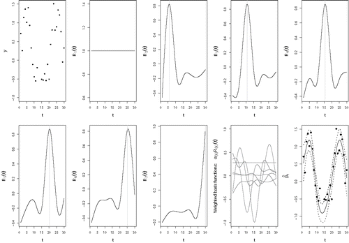
Figure 2. An example of a thin plate regression spline basis for the model y_t = β_t + ε_t. The basis functions for the smooth curve β_t of a thin plate regression spline basis are shown. The first panel represents the data through which the smooth curve will be fitted. The next two panels represent the first two basis functions, which are defined as R₁(t) = 1 and R₂(t) = t. The other five basis functions (R₃(t)–R₇(t)) are thin plate spline-specific basis functions. Just as in standard regression, all basis functions R_i(t) are weighed by multiplying them with their corresponding α_i coefficients. These weighted basis functions are then summed up, resulting in the smooth curve (with CI) in the last panel at the bottom right where the black dots again represent the data.

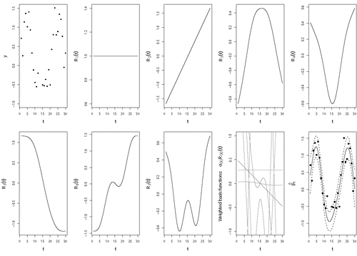
As a basis function, a polynomial basis (e.g., x⁰, x¹, x², etc.) could be used. However, in order to capture complicated nonlinear smooth terms, many of these basis functions need to be added. This would quickly lead to collinearity problems (Marra & Radice, 2010). To circumvent this problem, regression splines can be used as a basis. Regression splines are pieces of polynomials that are joined smoothly at breakpoints called knots (Hastie & Tibshirani, 1990). A common choice for regression splines are piecewise cubic polynomials, which are constrained to be continuous at the knot points and, additionally, are constrained to have a continuous first and second derivative (Fitzmaurice, Davidian, Verbeke, & Molenberghs, 2008). It is important to point out that although regression splines are segmented cubic polynomials joined at the knots, the function evaluation is not restricted to particular segments. Instead, there is an individual basis function for every knot and each basis function evaluates every value of t in the data (see Figure 1).

In the analyses of the current paper, we use the default regression spline basis of the GAM software: the thin plate regression spline basis (Wood, 2003, 2006). In contrast to cubic regression splines, where the basis functions are associated directly with a knot location, the basis functions in the thin plate regression splines are not knot-based in a conventional sense (see Figure 2). Instead, the thin plate regression spline approach starts with one knot per observation, using then an eigen-decomposition approach to get the number of basis coefficients maximally accounting for the variance in the data. Additionally, the basis functions are also no longer so sensitive to the exact knot placement (for more information, see Wood, 2003). Note also that in thin plate regression splines, every basis function that is added is “wigglier” than the previous basis function: for example, in Figure 2 basis function R₇ is wigglier than R₆. Different splines often give similar smooth functions and, thus, the choice of the spline basis is typically not crucial (Wood, 2006).

As stated previously, how complex or “wiggly” the final smooth function (e.g., ) becomes depends on the number of (regression spline) basis functions. By increasing the number of basis functions, the final smooth functions become more complex and “wiggly.” When using too few basis functions, the curve will have too little curvature and may not follow the data well. Too many basis functions, on the other hand, will lead to interpolation of the data points and will result in overfitting (Andersen, 2009; Keele, 2008). Thus, one crucial problem is finding the right number of basis functions.

One approach to find the right number of basis functions involves using the penalized likelihood approach (Wood, 2006). The idea behind this method is to take more basis functions than expected to be necessary and control the function’s smoothness by adding a wiggliness penalty (Wood, 2006). This penalty decreases the influence of the highly “wiggly” components of the basis functions. To determine the wiggliness penalty that leads to optimal smoothness of the function, a generalized cross-validation technique (GCV; Golub, Heath, & Wahba, 1979) can be used. The lowest GCV score represents the penalty that is optimal in the sense that it leads to the best trade-off between underfitting and overfitting.

All of the techniques described in this section are implemented in the mgcv package in R (Wood, 2006). Besides the type of spline bases, one only has to define enough basis functions, the default being 10 basis functions. The output contains the estimated smooth functions and a GCV score. The GAM procedure in the mgcv package also provides a measure of nonlinearity and 95% Bayesian credible intervals (CIs; see Wood, 2006). The measure of nonlinearity is the effective degrees of freedom (edf). An edf of one indicates a linear effect, and the higher the edf, the more “wiggly” the estimated smooth function (Shadish, Zuur, & Sullivan, 2014). The number of basis functions should be well below the maximum possible edf for the smooth function (or term) of interest (Wood, 2006). When this is not the case, the next step is to re-fit the model with a larger number of basis functions (e.g., double). If the reported edf increases substantially with this operation, this is a sign that even more basis functions are needed. Furthermore, the ref.df is given. This stands for the reference degrees of freedom and is an alternative measure of degrees of freedom, used for hypothesis testing. The 95% Bayesian credible intervals around the smooth curve reflect the uncertainty of the smooth function (for more details, see Wood, 2006).¹

Besides visually inspecting the plots of the intercept, autoregressive, and cross-lagged smooth functions to detect changes in the functions over time, it is possible to calculate fit indices such as the BIC and AIC for model comparison. Note that the BIC and AIC calculated for these penalized models are not maximizing the actual likelihood but penalized likelihood. Furthermore, to calculate the AIC and BIC, the edf is used instead of the actual number of parameters (see for more detailed information Hastie & Tibshirani, 1990). Following the results of a previous simulation study (Bringmann et al., 2017), we recommend to use only the BIC for model comparison when having over 100 time points. In these circumstances, the BIC functions well and can indicate whether a standard VAR model or one of the time-varying models fits the data better. Under 100 time points, neither the AIC nor the BIC performs particularly well in selecting the true model (i.e., whether the process under study is time-varying or time-invariant). The AIC will select the time-varying models too often, and the BIC will select the time-invariant (standard VAR) model too often. In this case, we recommend to use both the AIC and BIC, and to see if they converge to the same model. For more detailed information on model comparison between TV-(V)AR and standard (V)AR models, (see Bringmann et al., 2017).

5. Simulation study

To evaluate the performance of the TV-VAR model, we carried out a simulation study comparing a standard bivariate VAR to a bivariate TV-VAR model under different conditions of change using R,R (R Core Team, 2017). We investigated in which cases a TV-VAR model should be preferred over a standard VAR model by generating data from both models and evaluating their performances using the mean square error (MSE) and coverage probability of the 95% credibility intervals. The population parameters were based on previous studies (see, for example, Bos, Hoenders, & Jonge, 2012; Wigman et al., 2015).

5.1. Set up of the simulation study

There were two main conditions:

Figure 3. The three data-generating functions.

1.	The data are generated with a standard time-invariant VAR model in which the parameters do not change over time (see also Figure 3A): (8)
2.	The data are generated with a TV-VAR model (see also Figure 3B and 3C): (9)

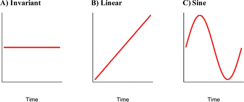
Parameters of the TV-VAR model could vary either as a linear function (Figure 3B) or as a sine function (Figure 3C). All parameters varied simultaneously over time. Both generating functions (the linear and the sine) varied from zero to a maximum (absolute) value (M). This value corresponded to the parameter values in the standard VAR model of Equation (8(8) ). In the case of a linear change, the time-varying parameter (e.g., β_{10, t}) was then simulated according to a linear function β_{10, t} = t · M/n, and in the sine case, the parameter was simulated according to a sine function , where n is the total number of time points, M is the maximum absolute value, and t_i denotes the time points i = 1, …, n.

In Figures 6 and 7, the line and tilde symbols represent how the parameters in the TV-VAR model changed over time (i.e., in a linear or sine way), the number in parentheses being the maximum absolute value of the time-varying parameter. For example, β_{10, t} varied as a linear function, the starting point being 0 and the end point being 1. As another example, parameter β_{22, t} varied as a sine function with the peak values being 0.3 and −0.3. Note that β_{12, t} did not vary over time as in this case the parameter value was 0. The innovations were simulated as a white-noise process, with the mean 0 and the following covariance matrix Σ: (10)

Besides the condition time-invariant/time-varying, we also varied the number of time points in the data (N = {61, 80, 100, 150, 200, 250, 300, 400, 1000}). In the last condition, we varied the number of basis functions: In addition to the default setting of 10 basis functions per smooth curve, we also halved and doubled the number of basis function, resulting in three extra conditions: 5, 10, and 20 basis functions. Note that for estimating a TV-VAR model with 2 variables and 20 basis functions, at least 61 time points are needed, as otherwise the model has more coefficients than data (e.g., 20 basis functions for each parameter (β_{10, t}, β_{11, t}, and β_{12, t}) leads to 60 coefficients per equation). Every condition was replicated 1000 times.

5.2. Estimation and evaluation

After the data were generated (with a VAR or TV-VAR model), they were fitted with (1) a VAR model and (2) a TV-VAR model using a thin plate regression spline basis using 5, 10 (the default setting), or 20 basis functions.

To evaluate the performance of the VAR and TV-VAR models, we calculated the average of the mean squared errors (MSEs) across the R = 1000 replications per condition. The MSE for a single time-varying coefficient can be defined as , where represents the estimated value at time point t, θ_t the true value at time point t, and n is the number of time points. Any of the parameters (i.e., and ) can take the role of θ_t. Additionally, a coverage probability was calculated, which is the proportion of time that the true value is captured by the confidence intervals in case a VAR model was fitted, or (Bayesian) credible intervals in case a TV-VAR model was fitted.

5.3. Results of the simulation study

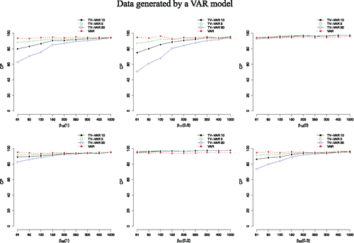
When the dynamics of the data were time-invariant (i.e., generated by a VAR model), the VAR model always did better (i.e., had a lower MSE value) than the TV-VAR model. For example, the relative efficiency or MSE ratio (i.e., MSE TV-VAR / MSE VAR) was around 7: 1 with 61 time points, meaning that the MSE of the TV-VAR model was seven times higher than that of the VAR model. Importantly, however, not only the MSE values of both models in general, but also the MSE ratio steeply decreased with more time points, reaching around 2.5: 1 with 1000 time points (see Figure 4). Moreover, even though the coverage probabilities were higher for the VAR model, from 200 time points on the coverage probabilities for the TV-VAR model reached good results with coverages over 90% (see Figure 5). Additionally, it is clear that when the number of time points is low, below 200, for example, having less basis functions (5 versus 10 or 20) results in more reliable estimates. This suggests that the penalization on the “wiggliness” of the smooth functions does not work ideally with a low number of time points. With more than 300 time points, the number of basis functions does not influence the results crucially anymore.

Figure 4. Average MSE values for both the TV-VAR (with 5, 10, and 20 basis functions) and the VAR model. The data were generated by the VAR model. A lower MSE value entails a better recovery of the true coefficient values. The number next to the β indicates its value.

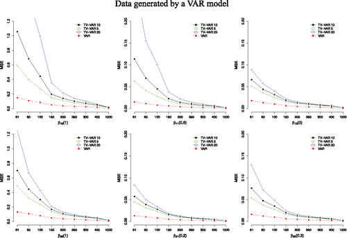
Figure 5. Average coverage probabilities (CP) in % for both the TV-VAR (with 5, 10, and 20 basis functions) and the VAR model. The data were generated by the VAR model. A higher value entails capturing the true coefficient values better. The number next to the β indicates its value. CIs for both models were 95%.

When the data were generated by a TV-VAR model as having time-varying dynamics, the TV-VAR model had in almost all cases a lower MSE value than the standard VAR model.² A TV-VAR model had always a better fit to the data when the change was pronounced, that is, when the absolute maximum value was high and the parameter changed as a sine instead of a linear function. In case of a linear change, the TV-VAR model detected change better than a VAR model from about 100 time points on (see Figure 6). In contrast, the coverage probabilities for the TV-VAR model were always better than for the VAR model regardless of the process of change. This difference increased as the number of time points increased. Importantly, the coverage probability of the TV-VAR model was in all cases above 90%, and this was the case already with 100 time points (see Figure 7). Also here the number of basis functions somewhat influenced the results when there were less than 150 time points. However, in most settings these differences were negligible.

Figure 6. Average MSE values for both the TV-VAR (with 5, 10, and 20 basis functions) and the VAR model. The data were generated by the TV-VAR model. A lower MSE value entails a better recovery of the true coefficient values. The number next to the β indicates the maximum absolute value of β and the symbols describe how β changed over time.

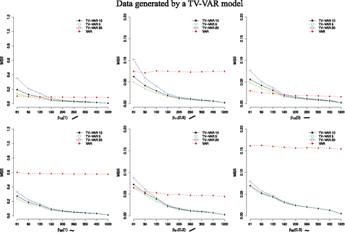
Figure 7. Average coverage probabilities (CP) in % for both the TV-VAR (with 5, 10, and 20 basis functions) and the VAR model. The data were generated by the TV-VAR model. A higher value entails capturing the true coefficient values better. The number next to the β indicates the maximum absolute value of β and the symbols describe how β changed over time. CIs for both models were 95%.

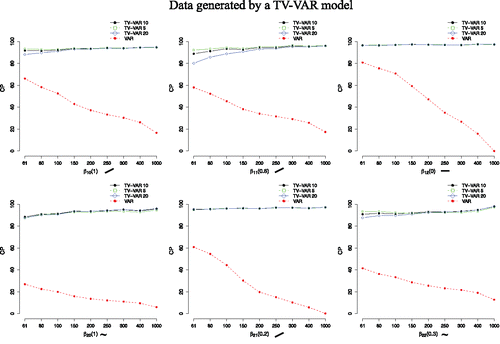
In conclusion, it seems that when it is suspected that time-varying dynamics in the data are present, a TV-VAR model is a preferable model from about 100 time points on. Furthermore, even if the dynamics are time-invariant, with at least 200 time points, a TV-VAR model gives good results.

6. Empirical example

6.1. Description

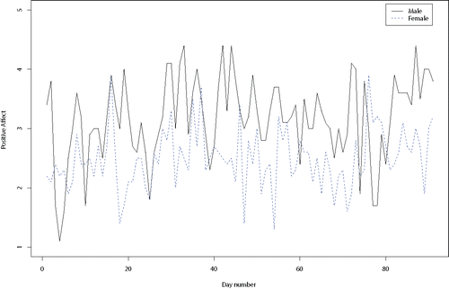
In this section, we apply our proposed approach to empirical data from two individuals in a dyad.³ In particular, to keep the example parsimonious, we focus on the feelings of positive affect (PA) in one couple that completed a daily questionnaire on their affect for 91 consecutive days (Figure 8; for more information see Ferrer, Widaman, Card, Selig, & Little, 2008; Ferrer, Steele, & Hsieh, 2012). Every day during the study period, the two individuals in the couple rated items representing emotion adjectives from the Positive and Negative Affective Schedule (PANAS; Watson, Clark, & Tellegen, 1988) responding to the instructions “Indicate to what extent you have felt this way today” on a 5-point likert scale, ranging from 1 (very slightly or not at all) to 5 (extremely). The 10 items representing positive affect (PA) included interested, excited, strong, enthusiastic, proud, inspired, determined, attentive, active, and alert. The PA score was based on the mean of these 10 items. The data are available on the website of the journal and the R-code to replicate the analyses can be found in the Appendix.

Figure 8. Daily positive affect (PA) scores for a male and a female involved in a romantic relationship.

6.2. Analysis

We carried out analyses using the TV-VAR model to study: (a) changes over time in PA for each individual in the dyad, and (b) the extent to which each individual’s PA was affected by the partner’s PA. The model of interest for our analyses is a model in which all terms are time-varying parameters (i.e., model 1 in Table 1): (11)

Table 1. The eight different models to select from for male and female positive affect.

Model			Model specification
Model 1		with
Model 2		with
Model 3		with
Model 4		with
Model 5		with
Model 6		with
Model 7		with
Model 8		with

Table 2. Time-varying VAR model selection for PA of the male. Lowest fit indices are made bold.

Model	AIC	BIC
Model 1		192.147
Model 2	172.995	195.185
Model 3	166.528	189.331
Model 4	172.600	195.396
Model 5	171.138	191.179
Model 6	174.169	192.636
Model 7	172.526	191.580
Model 8	178.813

This model was compared with alternative specifications, in other words, simpler models in which some or all of the parameters were time invariant (see model 2 until 8 in Table 1).

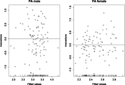
Model selection was based on three criteria: (1) significance level of the smooth parameters, (2) visual inspection of change in the parameters over time, and (3) AIC and BIC fit indices. For all models, the innovations ϵ_{1, t} and ϵ_{2, t} were evaluated, and tests indicated a lack of autocorrelation over time as well as homogeneity and a normal distribution (see, for example, the innovations of the first model depicted in Figure 9). We used the standard number of basis functions 10, and as a check, doubled the number of basis functions to 20 as well. Both settings gave highly similar results, and therefore 10 basis functions were used in the final model (see also the R-code in the Appendix).

Figure 9. Fitted values versus innovations of positive affect (PA) for both male and female. The innovations were homogenous and normally distributed.

6.3. Results

Both the time-varying and the standard VAR model indicated that all the parameters pertaining to the male’s PA were statistically significant, whereas those for the female’s PA were not. That is, in the emotion system of this dyad, only the male’s PA could be predicted over time. For example, the TV-VAR model, as depicted in model 1 and Equation (11(11) ), showed that the smoothing parameters for the male’s PA had p-values < 0.024 and were thus relevant for predicting his PA.

Regarding the question whether the parameters were time-varying or time-invariant, the AIC indices indicated that model 1, in which all parameters are time-varying, was the best model. In contrast, the BIC indicated the opposite: model 8, a standard VAR model where all the parameters are time-invariant, was the best fitting model (see Table 2).⁴

Interestingly^{Table 1, Table 2}, the second best model indicated by the AIC and BIC fit indices was in both cases model 3. In this model, the intercept and cross-lagged effect (female’s PA) were time-varying, whereas the autoregressive parameter (male’s PA) was not time-varying, but fixed to 0.25 with a p-value of 0.013. However, the differences in AIC values between model 1 and model 3 or BIC values between model 8 and model 3 were so small that the models can be seen as having an equivalent fit. Visual inspection of the smoothing parameters (see Figure 10) showed that, whereas the cross-lagged function is clearly varying over time, the autoregressive function (inertia) cannot be disregarded as a straight time invariant function, as it does not clearly go up or down at any point in time. In order to control for effects that are only due to differences in emotional variability, we also standardized the results (mean = 0 and variance = 1; see, for example, Bulteel et al., 2016). These analyses led to the same results and conclusions.

Figure 10. This figure shows the parameters of model 1 (Equation (11(11) )) for positive affect (PA) of the male and female. In model 1 all parameters were allowed to vary over time as smooth functions. The upper panel indicates, from left to right: (1) the intercept function, (2) the autoregressive function (or inertia) of PA of the male, and (3) the cross-lagged function (the effect of PA of the female on PA of the male). The lower panel has the same structure, but represents PA of the female, which could not be significantly predicted by her own PA nor the PA of her partner. Note that model 3 would result in the same figure, except for β_{11, t} and β_{21, t}, which in model 3 are constants of 0.25 and 0.06, respectively.

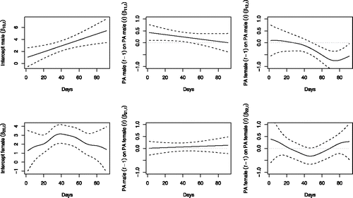
Thus, based on significance testing, visual inspection and fit indices, model 3 was chosen as the most plausible representation of the data. This means that the male in this couple had a stable emotional inertia over time, that is, he showed some spillover effects in his positive emotions from one day to the next. Furthermore, during the first part of the study, such emotions appeared to be mainly influenced by his own emotions. Halfway through the study, however, his emotions were also influenced by those of his female partner, but such effects were in the opposite direction. In other words, when her positive emotions were low, his tended to be higher the next day, and the other way around. Thus, a clear change in the dynamics between the partners was apparent in these data (see also Figure 10).

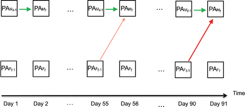
Whereas Figure 10 only represents the results of the TV-VAR model, it is also helpful to visually compare the results of a standard VAR model with those of a TV-VAR model. This is done in Figures 11 and 12, which are conceptual representations of how emotion dynamics are modeled in VAR and TV-VAR models, inspired by the network approach (see, for example, Borsboom & Cramer, 2013) and path analysis (see, for example, Loehlin, 2004). Figure 11 illustrates the VAR model, where the dynamics within and between the male and the female are time-invariant, whereas Figure 12 shows results of the TV-VAR model, where the interdependence in the dyad does change over time.

Figure 11. Conceptual representation of the VAR model for positive affect (PA) of the male and the female. In the VAR model the dynamics are not allowed to change over time.

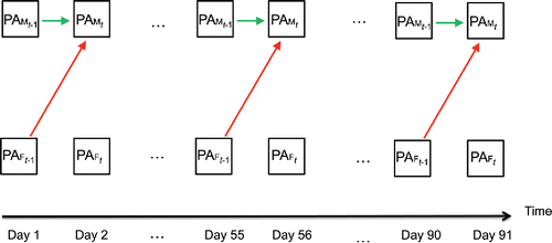
Figure 12. Conceptual representation of the TV-VAR model for positive affect (PA) of the male and the female. In the TV-VAR model, the dynamics are allowed to change over time. In this dyad, the dynamics did indeed change. There was initially no effect of the female’s PA on the male’s PA, but this cross-lagged effect appeared halfway through the study (see the thin red arrow) and got stronger over time (see the thick red arrow).

7. Discussion

Emotions arise in a social context. Very often they are elicited in the setting of interpersonal interactions, such as a dyad, the smallest possible group. While most models used to study these emotion dynamics assume stationarity, this is often an unrealistic assumption: Whether caused by an external event (e.g., divorce), or an internal force (e.g., rumination), emotion dynamics are prone to change.

In this article, we presented the TV-VAR, a model for exploring emotion dynamics and their changes over time, and showed its usefulness to examine dyadic interactions. Through a simulation study we demonstrated that, when the dynamics change smoothly over time, the TV-VAR model was superior to the standard time-invariant VAR model. Moreover, the results indicated that when the data were actually time-invariant, with at least 200 time points, the estimations of the TV-VAR model were still satisfactory.

We also applied the TV-VAR model to empirical data consisting of positive daily affect ratings from two individuals in a romantic relationship. In comparing the stationary VAR model to the TV-VAR model, we found evidence that the emotion dynamics within the couple varied over time. Specifically, we found that both the VAR and the TV-VAR model showed that the female’s positive affect was not influenced by her own affect, nor by that of her male partner. However, for the male’s positive affect, the results from the models differed. Whereas the VAR model indicated that the female’s positive affect always influenced the male’s, the TV-VAR model showed that her positive affect did not initially influence his positive affect, but such influence became evident halfway through the study. These results highlight the importance of using a TV-VAR model to identify changes in the dynamics in a system. For example, had stable autoregressive or cross-lagged effects been assumed, the change in dynamics would have been overseen.

The TV-VAR model is also applicable in other contexts. In fact, in all situations in which temporal dynamics can possibly alter over time, a TV-VAR model is potentially useful. For example, in the increasingly popular network approach to psychopathology, the networks are often inferred with a standard VAR model (Borsboom & Cramer, 2013; Bringmann et al., 2016; Fried et al., 2017; McNally, 2016; Pe et al., 2015; Wigman et al., 2015). However, many hypotheses underlying the network perspective involve change in the temporal dynamics. For instance, in the area of psychopathology, an increase in autocorrelation of the emotion dynamics, referred to as critical slowing down, is assumed to be an early warning for a transition into depression (van de Leemput et al., 2014). Translated to network theory, it is assumed that the network (i.e., autoregressive and cross-lagged parameters) gets more dense or strongly connected when a person transits to depression (Cramer et al., 2016). Whereas a VAR model would be unable to detect such shifts, a TV-VAR model could help to discover these important transitions.

An additional advantage of the TV-VAR model is that it can be used to detect nonstationarity. Even though there are tests to check for several kinds of stationarity (e.g., Dickey & Fuller, 1979), there is no direct test that checks for nonstationarity due to changes in the covariance structure (i.e., autoregressive and cross-lagged effects). Because the TV-VAR model can detect both dynamics that do and do not change over time, it can be used as an exploratory tool to check for nonstationarity due to changes in the covariance structure. Simultaneously, it can indicate whether trends in the data are present. Additionally, the TV-VAR model immediately captures how the covariance structure and trends in the data vary over time.

In this paper, we focused on the simplest TV-VAR model: a bivariate lag-1 model. A fruitful extension would be to include more variables and lags. More complex models, however, bring issues such as interpretability and the identification of false positive relations (e.g., Costantini et al., 2015; Rasmussen & Bro, 2012; Tibshirani, 1996). Future research should aim at developing regularization techniques for TV-VAR models in order to enhance model interpretability and to decrease the number of spurious connections (see, for example, Haslbeck & Waldorp, under review).

An important limitation of the TV-VAR model is that a relatively large number of time points (around 100) are needed in order to get reliable estimates. For physiological measurements (e.g., heart rate activity) such numbers are readily available. However, although self-report studies with a large number of time points are becoming more common, most such studies still collect far fewer than 100 time points (Rot, Hogenelst, & Schoevers, 2012; Trull & Ebner-Priemer, 2013). Furthermore, the TV-VAR model assumes the change to be gradual and abrupt changes cannot be identified. Such abrupt changes can be modeled using regime switching models (Hamaker et al., 2010), and future research should combine regime switching models with TV-VAR models in order to enable modeling both abrupt and gradual changes.

Additionally, as we estimate the TV-VAR model equation-by-equation, we are not explicitly estimating the innovation covariance. Note however, that this does not mean the model is based on the assumption that the covariance between the innovations is zero. In fact, it might very well be nonzero due to: (a) effects the variables have on one another at shorter intervals (i.e., lags), and (b) omitted variables that affect both variables (i.e., unobserved common causes). Thus, further development of techniques that allow us to study these innovation covariances can be of great interest.

Another limitation of the TV-VAR model is its idiographic approach. Future research should explore new ways to go beyond a single dyad, for example, by using a multilevel or a clustering approach. A multilevel version of the TV-VAR model would allow for estimating both intra- and inter-individual effects (Bringmann et al., 2013; Haan-Rietdijk, Gottman, Bergeman, & Hamaker, 2014; Schuurman, Ferrer, Boer-Sonnenschein, & Hamaker, 2016; Shiyko, Lanza, Tan, Li, & Shiffman, 2012; Snijders & Kenny, 1999; Winter & Wieling, 2016). A disadvantage of the multilevel approach, however, is that the individual effects are assumed to be drawn from a single distribution (usually the multivariate normal), limiting the amount of heterogeneity over individuals or dyads. In contrast, in a clustering approach, for every individual or dyad a separate model is estimated, making this approach very flexible. Clustering could then be conducted on the shape of the autoregressive and cross-lagged effects within the dyads (for a similar approach, see Heylen, Verduyn, Van Mechelen, & Ceulemans, 2015). Such clusters could be then meaningfully related to other dyad characteristics, such as relationship satisfaction, relationship duration, or personality traits of the partners. A disadvantage of the clustering approach is that more time points per individual are needed than with a multilevel approach, and that most clustering models have the unrealistic assumption of a perfect within-cluster homogeneity (however, an exception is De Roover, Ceulemans, Timmerman, & Onghena, 2013).

In the context of dyadic research, it is common practice to test for differences in autocorrelation or cross-lagged effects. A commonly used dyadic model, for instance, is the actor-partner model with two time points (Kenny & Cook, 1999; Kenny & Ledermann, 2010). In this model, hypotheses about the equivalences in “actor” (autoregressive) or “partner” (cross-lagged) effects can be tested by putting constraints on the model as the model is estimated in one go (for example, in a structural equation framework). The TV-VAR model, although more elaborated and flexible, has the limitation that the model is estimated separately for the two dyads under study. Although direct testing is not possible, one can compare “actor” or “partner” effects in an exploratory way, for example, by collating the standardized effect of interest of, in our case, the male and the female in one plot. As a preliminary test one could examine the credible intervals. If, for instance, the point estimate of the cross-lagged regression coefficient from the male to the female lies outside the credible interval for the cross-lagged coefficient from the female to the male, this is evidence for these effects being different.

The aim of this paper was to introduce the semi-parametric TV-VAR model into research on dyadic interactions and psychological research in general. We hope to have shown that the TV-VAR model is easy to apply and can detect and capture changing dynamics without prior knowledge of the nature of the change.

Article Information

Conflict of Interest Disclosures: Each author signed a form for disclosure of potential conflicts of interest. No authors reported any financial or other conflicts of interest in relation to the work described.

Ethical Principles: The authors affirm having followed professional ethical guidelines in preparing this work. These guidelines include obtaining informed consent from human participants, maintaining ethical treatment and respect for the rights of human or animal participants, and ensuring the privacy of participants and their data, such as ensuring that individual participants cannot be identified in reported results or from publicly available original or archival data.

Funding: This work was supported by the Consolidator Grant no. 647209 from the European Research Council (Denny Borsboom), the Belgian Federal Science Policy within the framework of the Interuniversity Attraction Poles program (IAP/P7/06), as well as by grant GOA/15/003 from the KU Leuven, and the grant G.0806.13 from the Research Foundation Flanders - FWO (Francis Tuerlinckx).

Role of the Funders/Sponsors: None of the funders or sponsors of this research had any role in the design and conduct of the study; collection, management, analysis, and interpretation of data; preparation, review, or approval of the manuscript; or decision to submit the manuscript for publication.

Acknowledgments: The authors would like to thank Markus Eronen for his comments on prior versions of this manuscript. The ideas and opinions expressed herein are those of the authors alone, and endorsement by the authors’ institutions or the funding agencies is not intended and should not be inferred.

Notes

1 It has recently also become possible to estimate generalized additive models in a fully Bayesian way (Wood, 2016).

2 Note that the MSE values sometimes seem to converge to exactly zero. This is not the case: with 1000 time points the estimates of, for example, the TV-VAR model get very precise, with MSE values around 0.005, but the values do not reach zero.

3 The dyad was selected from a larger pool of dyads. The criteria for selecting the couple were the availability of at least 80 time points and clearly time-varying parameters when estimating a TV-VAR model.

4 This was not a surprising result given simulations done in a previous study Bringmann et al. (2017), indicating that the AIC tends to choose time-varying models as the best model whereas the BIC indicates often time-invariant models as the best fitting model, especially when the number of time points is relatively small.

Appendix: R-code

 

###############################################################

################# General information #########################

###############################################################

# R-CODE for the manuscript BRINGMANN ET AL. 2018,

# Multivariate Behavioral Research.

# Title: Modeling nonstationary emotion dynamics in dyads using a

# semi-parametric time-varying vector-autoregressive model.

 

# The files needed are:

# data.txt

 

#%############################################%#

#%#####  Installing the libraries        #####%#

#%############################################%#

# Before you start you have to install and load the libraries below.

 

library(mgcv)# version 1.8-15

library(quantmod)# version 0.4-0

 

# Please make sure all files are in the same working directory

# and that you have set your working directory to source file location.

getwd()

ls() # Here you can see which files are in your current working directory.

 

#%############################################%#

#%#####  Loading the data                #####%#

#%############################################%#

 

data_subset<-read.table("data.txt", header=T,stringsAsFactors=F)

 

head(data_subset)#A first look at the data

# The first column represents the time points.

# The second column represents the positive affect (PA) of the male.

# The third column represent the positive affect (PA) of the female.

 

#%############################################%#

#%#####  Analyzing the data with TV-VAR  #####%#

#%############################################%#

 

tt=1:(dim(data_subset)[1])

 

# Here you simply lag your variables

pamL=Lag(as.numeric(data_subset$pam,1))# Lagging PA of the male

pafL=Lag(as.numeric(data_subset$paf,1))# Lagging PA of the female

 

 

# The actual TV-VAR analyses where all the parameters are time-varying:

# the intercept (s(tt)),

# the autoregressive s(tt,by=pamL) and

# cross-lagged parameter s(tt,by=pamf).

 

k=10#Here you can choose the number of basis functions

#It is clear from the edf and Ref.df that 5 basis functions is too few.

#The difference between 10, 15 and 20 basis functions is, however, negligible.

 

gam1<-gam(as.numeric(pam)~s(tt,k=k)+s(tt,by=pamL,k=k)+s(tt,by=pafL,k=k),

data=data_subset)

gam2<-gam(as.numeric(paf)~s(tt,k=k)+s(tt,by=pamL,k=k)+s(tt,by=pafL,k=k),

data=data_subset)

 

# Without the smoothing function s(tt,...) the parameters would be time-invariant

# as in standard regression.

# See also the paper and r-file of Bringmann et al. 2016

# "Changing dynamics: TV-AR models using generalized additive modeling"

# in Psychological Methods.

 

 

summary(gam1) #Predictability male PA

# The summary shows that all of the time-varying parameters are significant:

# Approximate significance of smooth terms:

#              edf Ref.df     F p-value

# s(tt)       1.00  1.000 8.087 0.00562 **

# s(tt):pagmL 2.00  2.000 3.925 0.02355 *

# s(tt):pagfL 5.65  6.724 3.480 0.00303 **

 

# To see how the intercept, autoregressive and cross-lagged effects change over

# time, we would have to plot the functions (see next section).

# The effective degrees of freedom (edf) gives us information on

# how wiggly the smooth function is.

# The edf of the autoregressive smooth function has an edf of 2,

# and could indicate either a straight time-invariant line or a linear increase.

# The cross-lagged effect is clearly more wiggly and has an edf of over 5.

 

 

summary(gam2) #Predictability female PA

# The summary shows that none of the time-varying parameters are significant:

 

# Approximate significance of smooth terms:

#               edf Ref.df     F p-value

# s(tt)       5.836  6.731 0.785   0.600

# s(tt):pagmL 2.000  2.000 0.359   0.700

# s(tt):pagfL 4.735  5.436 0.875   0.482

 

# This can also be seen in the plots.

# There is always a zero is included in the CI:

plot(gam2, select=2,ylim=c(-1,1),rug=F,xlab="Days",

     ylab=substitute(paste("PA male",italic("(t-1)"),

                           "on PA female",italic("(t)"))))

plot(gam2, select=3,ylim=c(-1,1),rug=F,xlab="Days",

     ylab=substitute(paste("PA female",italic("(t-1)"),

                           "on PA female",italic("(t)"))))

 

 

 

#%#############################################%#

#%##### Figure of the main results in the paper #

#%#############################################%#

 

pdf("PA_FigureTVVAR.pdf",w=8.42,h=5)

par(mfrow=c(2,3))

par(oma=c(1,1,1,1))

 

numb=1

plot(gam1,rug=FALSE,select=1,seWithMean=TRUE,

     shift=coef(gam1)[1],xlab="Days",

     cex.lab = numb, cex.axis = numb,

     ylab=bquote(paste(Intercept~male~(italic(beta[10][","][t])))))

 

plot(gam1,select=2,ylim=c(-1,1),rug=F,xlab="Days",

     cex.lab = numb, cex.axis = numb,

     ylab=bquote(paste(PA~male~(italic(t-1))~on~PA~male~

     (italic(t)))~(italic(beta[11][","][t]))))

lines(tt,rep(0,91),col="darkgrey",lty=3)

 

plot(gam1,select=3,ylim=c(-1,1),rug=F,xlab="Days",cex.lab = numb, cex.axis = numb,

     ylab=bquote(paste(PA~female~(italic(t-1))~on~PA~male~

     (italic(t)))~(italic(beta[12][","][t]))))

lines(tt,rep(0,91),col="darkgrey",lty=3)

 

 

plot(gam2,rug=FALSE,select=1,seWithMean=TRUE,shift=coef(gam2)[1],xlab="Days",

     cex.lab = numb, cex.axis = numb,

     ylab=bquote(paste(Intercept~female~(italic(beta[20][","][t])))))

 

plot(gam2,select=2,ylim=c(-1,1),rug=F,xlab="Days",cex.lab = numb, cex.axis = numb,

     ylab=bquote(paste(PA~male~(italic(t-1))~on~PA~female~(italic(t)))~

     (italic(beta[21][","][t]))))

lines(tt,rep(0,91),col="darkgrey",lty=3)

 

plot(gam2,select=3,ylim=c(-1,1),rug=F,xlab="Days",cex.lab = numb, cex.axis = numb,

     ylab=bquote(paste(PA~female~(italic(t-1))~on~PA~female~(italic(t)))~

     (italic(beta[22][","][t]))))

lines(tt,rep(0,91),col="darkgrey",lty=3)

 

 

dev.off()

References

- aan het Rot, M., Hogenelst, K., & Schoevers, R. A. (2012). Mood disorders in everyday life: A systematic review of experience sampling and ecological momentary assessment studies. Clinical Psychology Review, 32(6), 510–523. doi: 10.1016/j.cpr.2012.05.007
- Andersen, R. (2009). Nonparametric methods for modeling nonlinearity in regression analysis. Annual Review of Sociology, 35, 67–85. doi: 10.1146/annurev.soc.34.040507.134631
- Boker, S. M., Cohn, J. F., Theobald, B.-J., Matthews, I., Mangini, M., Spies, J. R., .. Brick, T. R. (2011). Something in the way we move: Motion dynamics, not perceived sex, influence head movements in conversation. Journal of Experimental Psychology: Human Perception and Performance, 37(3), 874–891. doi: 10.1037/a0021928
- Boker, S. M., & Laurenceau, J.-P. (2006). Dynamical systems modeling: An application to the regulation of intimacy and disclosure in marriage. In T. A. Walls & J. L. Schafer (Eds.), Models for intensive longitudinal data (pp. 195–218). Oxford, England: Oxford University Press.
- Boker, S. M., & Nesselroade, J. R. (2002). A method for modeling the intrinsic dynamics of intraindividual variability: Recovering the parameters of simulated oscillators in multi-wave panel data. Multivariate Behavioral Research, 37(1), 127–160. doi: 10.1207/S15327906MBR3701_06
- Boker, S. M., Rotondo, J. L., Xu, M., & King, K. (2002). Windowed cross-correlation and peak picking for the analysis of variability in the association between behavioral time series. Psychological Methods, 7(3), 338–355. doi: 10.1037//1082-989X.7.3.338
- Borsboom, D., & Cramer, A. O. (2013). Network analysis: An integrative approach to the structure of psychopathology. Annual Review of Clinical Psychology, 9, 91–121. doi: 10.1146/annurev-clinpsy-050212-185608
- Bos, E. H., Hoenders, R., & de Jonge, P. (2012). Wind direction and mental health: A time-series analysis of weather influences in a patient with anxiety disorder. BMJ Case Reports, 2012. doi: 10.1136/bcr-2012-006300.
- Brandt, P. T., & Williams, J. T. (2007). Multiple time series models. Series: Quantitative applications in the social sciences. Thousand Oaks, CA: Sage Publications Inc.
- Bringmann, L. F., Hamaker, E. L., Vigo, D. E., Aubert, A., Borsboom, D., & Tuerlinckx, F. (2017). Changing dynamics: Time-varying autoregressive models using generalized additive modeling. Psychological Methods, 22(3), 409–425. doi: 10.1037/met0000085
- Bringmann, L. F., Lemmens, L. H., Huibers, M. J., Borsboom, D., & Tuerlinckx, F. (2015). Revealing the dynamic network structure of the Beck Depression Inventory-II. Psychological Medicine, 45(04), 747–757. doi: 10.1017/S0033291714001809
- Bringmann, L. F., Madeline, L. P., Vissers, N., Ceulemans, E., Borsboom, D., Vanpaemel, W., .. Kuppens, P. (2016). Assessing temporal emotion dynamics using networks. Assessment, 23(4), 425–435. doi: 10.1177/1073191116645909
- Bringmann, L. F., Vissers, N., Wichers, M., Geschwind, N., Kuppens, P., Peeters, F., .. Tuerlinckx, F. (2013). A network approach to psychopathology: New insights into clinical longitudinal data. PloS One, 8(4), e60188. doi: 10.1371/journal.pone.0060188
- Bulteel, K., Tuerlinckx, F., Brose, A., & Ceulemans, E. (2016). Using raw VAR regression coefficients to build networks can be misleading. Multivariate Behavioral Research, 51(2–3), 330–344. doi: 10.1080/00273171
- Butler, E. A. (2011). Temporal interpersonal emotion systems: The “TIES” that form relationships. Personality and Social Psychology Review, 15(4), 367–393. doi: 10.1177/1088868311411164
- Chatfield, C. (2003). The analysis of time series: An introduction (5th ed.). Boca Raton, FL: Chapman and Hall/CRC.
- Chow, S.-M., Lu, O., Cohn, J., & Messinger, D. (2017). Representing self-organization and non-stationarities in dyadic interaction processes using dynamic systems modeling techniques. In A. Von Davier & P. Kyllonen (Eds.), Innovative assessment of collaboration (pp. 269–286). New York, NY: Springer.
- Chow, S.-M., Zu, J., Shifren, K., & Zhang, G. (2011). Dynamic factor analysis models with time-varying parameters. Multivariate Behavioral Research, 46(2), 303–339. doi: 10.1080/00273171.2011.563697
- Costantini, G., Epskamp, S., Borsboom, D., Perugini, M., Mõttus, R., Waldorp, L. J., & Cramer, A. O. (2015). State of the aRt personality research: A tutorial on network analysis of personality data in R. Journal of Research in Personality, 54, 13–29. doi: 10.1016/j.jrp.2014.07.003
- Cramer, A., van Borkulo, C., Giltay, E., van der Maas, H., Kendler, K., Scheffer, M., … Borsboom, D. (2016). Major depression as a complex dynamical system. PLoS ONE, 11, e0167490.
- Dahlhaus, R. (1997). Fitting time series models to nonstationary processes. The Annals of Statistics, 25(1), 1–37. doi: 10.1214/aos/1034276620
- de Haan-Rietdijk, S., Gottman, J. M., Bergeman, C. S., & Hamaker, E. L. (2014). Get over it! A multilevel threshold autoregressive model for state-dependent affect regulation. Psychometrika, 81(1), 217–241. doi: 10.1007/s11336-014-9417-x
- De Roover, K., Ceulemans, E., Timmerman, M. E., & Onghena, P. (2013). A clusterwise simultaneous component method for capturing within-cluster differences in component variances and correlations. British Journal of Mathematical and Statistical Psychology, 66(1), 81–102. doi: 10.1111/j.2044-8317.2012.02040.x
- Dickey, D. A., & Fuller, W. A. (1979). Distribution of the estimators for autoregressive time series with a unit root. Journal of the American Statistical Association, 74(366a), 427–431. doi: 10.1080/01621459.1979.10482531
- Felmlee, D. H., & Greenberg, D. F. (1999). A dynamic systems model of dyadic interaction. The Journal of Mathematical Sociology, 23(3), 155–180. doi: 10.1080/0022250X.1999.9990218
- Ferrer, E. (2006). Application of dynamic factor analysis to affective processes in dyads. In A. Ong & M. van Dulmen (Eds.), Handbook of methods in positive psychology (pp. 41–58). Oxford, UK: Oxford University Press.
- Ferrer, E. (2016). Exploratory approaches for studying social interactions, dynamics, and multivariate processes in psychological science. Multivariate Behavioral Research, 51(2–3), 240–256. doi: 10.1080/00273171.2016.1140629
- Ferrer, E., & Nesselroade, J. R. (2003). Modeling affective processes in dyadic relations via dynamic factor analysis. Emotion, 3(4), 344–360. doi: 10.1037/1528-3542.3.4.344
- Ferrer, E., Steele, J. S., & Hsieh, F. (2012). Analyzing the dynamics of affective dyadic interactions using patterns of intra-and interindividual variability. Multivariate Behavioral Research, 47(1), 136–171. doi: 10.1080/00273171.2012.640605
- Ferrer, E., Widaman, K. F., Card, N., Selig, J., & Little, T. (2008). Dynamic factor analysis of dyadic affective processes with inter-group differences. In N. Card, J. Selig, & T. Little (Eds.), Modeling dyadic and interdependent data in the developmental and behavioral sciences (pp. 107–137). Hillsdale, NJ: Psychology Press.
- Ferrer, E., & Zhang, G. (2009). Time series models for examining psychological processes: Applications and new developments. In R. E. Millsap & A. Maydeu-Olivares (Eds.), Handbook of quantitative methods in psychology (pp. 637–657). London: Sage Publications.
- Fitzmaurice, G., Davidian, M., Verbeke, G., & Molenberghs, G. (2008). Longitudinal data analysis. Boca Raton, FL: Chapman and Hall/CRC.
- Fried, E. I., Borkulo, C. D. van, Cramer, A. O., Boschloo, L., Schoevers, R. A., & Borsboom, D. (2017). Mental disorders as networks of problems: A review of recent insights. Social Psychiatry and Psychiatric Epidemiology, 52(1), 1–10. doi: 10.1007/s00127-016-1319-z
- Frühwirth-Schnatter, S. (2006). Finite mixture and Markov switching models: Modeling and applications to random processes. New York: Springer.
- Giraitis, L., Kapetanios, G., & Yates, T. (2014). Inference on stochastic time-varying coefficient models. Journal of Econometrics, 179(1), 46–65. doi: 10.1016/j.jeconom.2013.10.009
- Golub, G. H., Heath, M., & Wahba, G. (1979). Generalized cross-validation as a method for choosing a good ridge parameter. Technometrics, 21(2), 215–223. doi: 10.1080/00401706.1979.10489751
- Gottman, J. M. (1979). Marital interaction: Experimental investigations. New York: Academic Press.
- Gottman, J. M. (2003). The mathematics of marriage: Dynamic nonlinear models. Cambridge: MIT Press.
- Gottman, J. M., Coan, J., Carrere, S., & Swanson, C. (1998). Predicting marital happiness and stability from newlywed interactions. Journal of Marriage and Family, 60(1), 5–22. doi: 10.2307/353438
- Gottman, J. M., & Levenson, R. W. (1986). Assessing the role of emotion in marriage. Behavioral Assessment, 8(1), 31–48.
- Gottman, J. M., & Levenson, R. W. (1992). Marital processes predictive of later dissolution: Behavior, physiology, and health. Journal of Personality and Social Psychology, 63(2), 221–233.
- Gottman, J. M., Swanson, C., & Swanson, K. (2002). A general systems theory of marriage: Nonlinear difference equation modeling of marital interaction. Personality and Social Psychology Review, 6(4), 326–340. doi: 10.1207/S15327957PSPR0604_07
- Hamaker, E. L., Grasman, R. P. P. P., & Kamphuis, J. H. (2010). Regime-switching models to study psychological processes. In P. C. M. Molenaar & K. Newell (Eds.), Individual pathways of change (pp. 155–168). Washington, DC: American Psychological Association.
- Hamaker, E. L., Kuiper, R. M., & Grasman, R. P. (2015). A critique of the cross-lagged panel model. Psychological Methods, 20(1), 102–116. doi: 10.1037/a0038889
- Hamaker, E. L., Zhang, Z., & van der Maas, H. L. (2009). Using threshold autoregressive models to study dyadic interactions. Psychometrika, 74(4), 727–745. doi: 10.1007/s11336-009-9113-4
- Hamilton, J. D. (1994). Time series analysis. Princeton, NJ: Princeton university press.
- Haslbeck, J., & Waldorp, L. (under review). MGM: Structure estimation for time-varying mixed graphical models in high-dimensional data.
- Hastie, T. J., & Tibshirani, R. J. (1990). Generalized additive models. Boca Raton, FL: Chapman and Hall/CRC.
- Heylen, J., Verduyn, P., Van Mechelen, I., & Ceulemans, E. (2015). Variability in anger intensity profiles: Structure and predictive basis. Cognition and Emotion, 29(1), 168–177. doi: 10.1080/02699931.2014.896783
- Hsieh, F., Ferrer, E., Chen, S.-C., & Chow, S.-M. (2010). Exploring the dynamics of dyadic interactions via hierarchical segmentation. Psychometrika, 75(2), 351–372. doi: 10.1007/s11336-009-9146-8
- Keele, L. J. (2008). Semiparametric regression for the social sciences. Chichester, England: John Wiley & Sons.
- Keltner, D., & Haidt, J. (1999). Social functions of emotions at four levels of analysis. Cognition and Emotion, 13(5), 505–521. doi: 10.1080/026999399379168
- Kenny, D. A., & Cook, W. (1999). Partner effects in relationship research: Conceptual issues, analytic difficulties, and illustrations. Personal Relationships, 6(4), 433–448. doi: 10.1111/j.1475-6811.1999.tb00202.x
- Kenny, D. A., & Ledermann, T. (2010). Detecting, measuring, and testing dyadic patterns in the actor–partner interdependence model. Journal of Family Psychology, 24(3), 359–366. doi: 10.1037/a0019651.
- Koval, P., Butler, E. A., Hollenstein, T., Lanteigne, D., & Kuppens, P. (2015). Emotion regulation and the temporal dynamics of emotions: Effects of cognitive reappraisal and expressive suppression on emotional inertia. Cognition and Emotion, 29(5), 831–851. doi: 10.1080/02699931.2014.948388
- Koval, P., & Kuppens, P. (2012). Changing emotion dynamics: Individual differences in the effect of anticipatory social stress on emotional inertia. Emotion, 12(2), 256–267. doi: 10.1037/a0024756
- Kuppens, P., Allen, N. B., & Sheeber, L. B. (2010). Emotional inertia and psychological maladjustment. Psychological Science, 21, 984–991. doi: 10.1177/0956797610372634
- Kuppens, P., Sheeber, L. B., Yap, M. B., Whittle, S., Simmons, J. G., & Allen, N. B. (2012). Emotional inertia prospectively predicts the onset of depressive disorder in adolescence. Emotion, 12(2), 283–289. doi: 10.3389/fpsyg.2012.00380
- Kuppens, P., Stouten, J., & Mesquita, B. (2009). Individual differences in emotion components and dynamics: Introduction to the special issue. Cognition and Emotion, 23(7), 1249–1258. doi: 10.1080/02699930902985605
- Larson, R. W., & Almeida, D. M. (1999). Emotional transmission in the daily lives of families: A new paradigm for studying family process. Journal of Marriage and Family, 61, 5–20. doi: 10.2307/353879
- Lebo, M. A., & Nesselroade, J. R. (1978). Intraindividual differences dimensions of mood change during pregnancy identified in five p-technique factor analyses. Journal of Research in Personality, 12(2), 205–224. doi: 10.1016/0092-6566(78)90098-3
- Liu, S., & Molenaar, P. (2016). Testing for granger causality in the frequency domain: A phase resampling method. Multivariate behavioral research, 51(1), 53–66. doi: 10.1080/00273171.2015.1100528
- Loehlin, J. C. (2004). Latent variable models: An introduction to factor, path, and structural analysis (4th ed.). Mahwah, NJ: Lawrence Erlbaum Associates Publishers.
- Lütkepohl, H. (2007). New introduction to multiple time series analysis. New York: Springer.
- Madhyastha, T. M., Hamaker, E. L., & Gottman, J. M. (2011). Investigating spousal influence using moment-to-moment affect data from marital conflict. Journal of Family Psychology, 25(2), 292–300. doi: 10.1037/a0023028
- Marra, G., & Radice, R. (2010). Penalised regression splines: Theory and application to medical research. Statistical Methods in Medical Research, 19(2), 107–125. doi: 10.1177/0962280208096688
- McNally, R. J. (2016). Can network analysis transform psychopathology? Behaviour Research and Therapy, 86, 95–104.doi: 10.1016/j.brat.2016.06.006.
- Molenaar, P. C. M., De Gooijer, J. G., & Schmitz, B. (1992). Dynamic factor analysis of nonstationary multivariate time series. Psychometrika, 57(3), 333–349.
- Parkinson, B. (1996). Emotions are social. British Journal of Psychology, 87(4), 663–683. doi: 10.1111/j.2044-8295.1996.tb02615.x
- Pe, M. L., Kircanski, K., Thompson, R. J., Bringmann, L. F., Tuerlinckx, F., Mestdagh, M., .. Gotlib, I. H. (2015). Emotion-network density in major depressive disorder. Clinical Psychological Science, 3(2), 292–300. doi: 10.1177/2167702614540645
- R Core Team (2017). R: A language and environment for statistical computing. R Foundation for Statistical Computing. Vienna, Austria. Available at http://www.R-project.org/.
- Randall, A. K., & Butler, E. A. (2013). Attachment and emotion transmission within romantic relationships: Merging intrapersonal and interpersonal perspectives. Journal of Relationships Research, 4, e10. doi: 10.1017/jrr.2013.10
- Rasmussen, M. A., & Bro, R. (2012). A tutorial on the lasso approach to sparse modeling. Chemometrics and Intelligent Laboratory Systems, 119, 21–31. doi: 10.1016/j.chemolab.2012.10.003
- Sadler, P., Ethier, N., Gunn, G. R., Duong, D., & Woody, E. (2009). Are we on the same wavelength? Interpersonal complementarity as shared cyclical patterns during interactions. Journal of Personality and Social Psychology, 97(6), 1005–1020. doi: 10.1037/a0016232
- Schuurman, N. K., Ferrer, E., Boer-Sonnenschein, M. de, & Hamaker, E. L. (2016). How to compare cross-lagged associations in a multilevel autoregressive model. Psychological Methods, 21(2), 206–261. doi: 10.1037/met0000062
- Shadish, W. R., Zuur, A. F., & Sullivan, K. J. (2014). Using generalized additive (mixed) models to analyze single case designs. Journal of School Psychology, 52(2), 149–178. doi: 10.1016/j.jsp.2013.11.004
- Shiyko, M. P., Lanza, S. T., Tan, X., Li, R., & Shiffman, S. (2012). Using the time-varying effect model (TVEM) to examine dynamic associations between negative affect and self confidence on smoking urges: Differences between successful quitters and relapsers. Prevention Science, 13(3), 288–299. doi: 10.1007/s11121-011-0264-z
- Snijders, T. A., & Kenny, D. A. (1999). The social relations model for family data: A multilevel approach. Personal Relationships, 6(4), 471–486. doi: 10.1111/j.1475-6811.1999.tb00204.x
- Steele, J. S., & Ferrer, E. (2011). Latent differential equation modeling of self-regulatory and coregulatory affective processes. Multivariate Behavioral Research, 46(6), 956–984. doi: 10.1080/00273171.2011.625305
- Stifter, C. A., & Rovine, M. (2015). Modeling dyadic processes using hidden markov models: A time series approach to mother–infant interactions during infant immunization. Infant and Child Development, 24(3), 298–321. doi: 10.1002/icd.1907.
- Suls, J., Green, P., & Hillis, S. (1998). Emotional reactivity to everyday problems, affective inertia, and neuroticism. Personality and Social Psychology Bulletin, 24(2), 127–136. doi: 10.1177/0146167298242002
- Tibshirani, R. (1996). Regression shrinkage and selection via the lasso. Journal of the Royal Statistical Society. Series B (Methodological), 58, 267–288.
- Trull, T. J., & Ebner-Priemer, U. (2013). Ambulatory assessment. Annual Review of Clinical Psychology, 9, 151–176. doi: 10.1146/annurev-clinpsy-050212-185510
- van de Leemput, I. A., Wichers, M., Cramer, A., Borsboom, D., Tuerlinckx, F., Kuppens, P., .. Scheffer, M. (2014). Critical slowing down as early warning for the onset and termination of depression. Proceedings of the National Academy of Sciences, 111(1), 87–92. doi: 10.1073/pnas.1312114110
- Watson, D., Clark, L. A., & Tellegen, A. (1988). Development and validation of brief measures of positive and negative affect: The PANAS scales. Journal of Personality and Social Psychology, 54(6), 1063–1070. doi: 10.1037/0022-3514.54.6.1063
- Wigman, J., van Os, J., Borsboom, D., Wardenaar, K., Epskamp, S., Klippel, A., .. Wichers, M. (2015). Exploring the underlying structure of mental disorders: Cross-diagnostic differences and similarities from a network perspective using both a top-down and a bottom-up approach. Psychological Medicine, 45(11), 2375–2387. doi: 10.1017/S0033291715000331
- Winter, B., & Wieling, M. (2016). How to analyze linguistic change using mixed models, growth curve analysis and generalized additive modeling. Journal of Language Evolution, 1(1), 7–18. doi: 10.1093/jole/lzv003
- Wood, S. N. (2000). Modelling and smoothing parameter estimation with multiple quadratic penalties. Journal of the Royal Statistical Society: Series B (Statistical Methodology), 62(2), 413–428. doi: 10.1111/1467-9868.00240
- Wood, S. N. (2003). Thin plate regression splines. Journal of the Royal Statistical Society: Series B (Statistical Methodology), 65(1), 95–114. doi: 10.1111/1467-9868.00374
- Wood, S. N. (2006). Generalized additive models: An introduction with R. Boca Raton, FL: Chapman and Hall/CRC.
- Wood, S. N. (2016). Just another gibbs additive modeler: Interfacing JAGS and mgcv. Journal of Statistical Software, 75(1), 1–15. doi: 10.18637/jss.v075.i07