Investigating the Utility of Fixed-margin Sampling in Network Psychometrics

Abstract

Steinley, Hoffman, Brusco, and Sher (2017) proposed a new method for evaluating the performance of psychological network models: fixed-margin sampling. The authors investigated LASSO regularized Ising models (eLasso) by generating random datasets with the same margins as the original binary dataset, and concluded that many estimated eLasso parameters are not distinguishable from those that would be expected if the data were generated by chance. We argue that fixed-margin sampling cannot be used for this purpose, as it generates data under a particular null-hypothesis: a unidimensional factor model with interchangeable indicators (i.e., the Rasch model). We show this by discussing relevant psychometric literature and by performing simulation studies. Results indicate that while eLasso correctly estimated network models and estimated almost no edges due to chance, fixed-margin sampling performed poorly in classifying true effects as “interesting” (Steinley et al. 2017, p. 1004). Further simulation studies indicate that fixed-margin sampling offers a powerful method for highlighting local misfit from the Rasch model, but performs only moderately in identifying global departures from the Rasch model. We conclude that fixed-margin sampling is not up to the task of assessing if results from estimated Ising models or other multivariate psychometric models are due to chance.

Keywords:

• exploratory data analysis
• IRT
• network Psychometrics
• Ising models
• fixed-margin sampling

Investigating the utility of fixed-margin sampling in network psychometrics

The field of network psychometrics (Marsman et al., 2018), which aims to estimate graphical models (represented visually as networks) from psychological data, has grown popular in recent years. In a commentary on a target article (Forbes, Wright, Markon, & Krueger, 2017a) relating to the replicability of network models, Steinley, Hoffman, Brusco, & Sher (2017) proposed a new method for evaluating the performance of psychopathological network models estimated from binary data. The method takes a binary dataset and resamples random values while keeping both the row and column margins intact in order to obtain intervals around any parameter. We will term this method fixed-margin sampling. The focus of Steinley et al.’s (2017) commentary was on LASSO regularized Ising models (eLasso; van Borkulo et al., 2014). The target article’s conclusion was that these networks “have limited replicability,” (p. 969) but in a comprehensive re-analysis, Borsboom et al. (2017) showed that replicability of eLasso Ising networks was in fact very good. Steinley et al. (2017), on the other hand, re-evaluated one of the datasets using their newly proposed method and determined that “many of the results are indistinguishable from what would be expected by chance” (p. 1000), labeled such findings “uninteresting” (p. 1004), and suggested that “previously published findings using [eLasso] should be reevaluated using the above testing procedure” (p. 1008). In a rebuttal to the re-analysis of Borsboom et al. (2017), Forbes, Wright, Markon, & Krueger (2017b) rely, in part, on the results of Steinley et al. (2017) by taking these findings as further evidence that methods such as eLasso have “limited replicability and utility” (p. 1011).

As the conclusions of Steinley et al. (2017) may have considerable implications for the eLasso method and research from different disciplines on which this methodology is based (e.g., Agresti, 1990; Barber & Drton 2015; Hastie, Tibshirani, & Friedman, 2001; Hastie, Tibshirani, & Wainwright, 2015; Meinshausen & Bühlmann, 2006; Pearl, 2000; Tibshirani, 1996; van Borkulo & Epskamp, 2014), we set out to evaluate the proposed fixed-margin sampling method. On the basis of this examination, we conclude that fixed-margin sampling leads to data being generated under a very specific null-hypothesis (i.e., unidimensionality with interchangeable indicators; the Rasch model), rather than under random chance. The null-distribution therefore imposes a strong structure on the generated data-matrices that cannot be considered random, especially in light of known model equivalences between Rasch models and Ising models (e.g., Marsman et al., 2018). As such, if the aim is “to distinguish [empirical findings] from random chance” (Steinley et al., 2017, p. 1008), fixed-margin sampling will provide an inappropriate null-hypothesis.

The remainder of this article is outlined as follows. First, we discuss the methodology and its origin, followed by a description of relevant psychometric literature and an explanation why the null-hypothesis of fixed-margin sampling method is inappropriate for assessing if parameters are due to chance. Second, we discuss why fixed-margin sampling is powerful in the analysis of networks connecting two sets of entities (e.g., actors and movies), but perform poorly when applied to networks of random variables (e.g., symptoms). Third, we evaluate the utility of fixed-margin sampling both in assessing parameters of the Ising model as well as assessing Rasch models in simulation studies. Finally, we re-evaluate the results presented by Steinley et al. (2017) in light of our conclusions regarding the utility of the method in network psychometrics.

Fixed-margin sampling

Steinley et al. (2017) propose to (1) simulate 1,000 random binary matrices with the same dimensions and margins (row and column sum-scores) as the original data, (2) compute a network structure for each generated dataset, (3) derive a relevant statistic (e.g., edge weight or centrality index) from each of these networks, (4) order the repeated samples of the statistic, (5) take the 5th and 995th ordered sample to create an interval,1¹ and (6) check if the observed statistic lies within the computed interval. In their reported Table 1, Steinley et al. are very clear on the interpretation of results from this method. If an edge-weight (or any other statistic) lies within this interval, it is classified as “uninteresting” (p. 1004). If it is not in this interval, it is classified as “potentially interesting” (p. 1004). For example, suppose we observe an estimated edge weight of 0.3 between two nodes. Next, we can resample the data-matrix, while keeping both row- and column-totals fixed to the original margins (sample people that endorse the same number of items, and sample variables that are endorsed by the same number of people), to generate 1,000 networks leading to 1,000 repetitions of the edge estimate in question. Suppose the 5th ordered sample is 0.1 and the 995th ordered sample is 0.5. Steinley et al. (2017) would deem the estimated edge-weight of 0.3 “uninteresting” (p. 1004). While we argue against this interpretation in this article, we retain the terminology in line with Steinley et al. (2017) throughout the remainder of this article. We use the term “(potentially) interesting” to describe an edge for which the observed weight lies outside that of the interval created using fixed-margin sampling. We use the term “uninteresting” to describe an edge for which the observed weight lies within (or is equal to the boundary of) the interval obtained using fixed-margin sampling.

Table 1. Possible outcomes of estimated edges in a model.

	Edge present in true model	Edge absent in true model
Edge present in estimated model	True positive	False positive (Type I error)
Edge absent in estimated model	False negative (Type II error)	True negative

The estimation procedure works correctly if it mostly estimates true positives or true negatives. In the case of a false positive (Type I error), the presence of an edge in the estimated model is due to chance. In the case of a false negative (Type II error), the estimation procedure lacked statistical power to detect the true edge.

The inspiration for the procedure suggested by Steinley et al. (2017) comes from the ecology literature (Connor & Simberloff, 1979). Suppose we have data of several species of birds (rows in a dataset), which live or do not live on a set of islands (columns in a dataset). We may encode with a 1 if a type of bird lives on an island, and with a 0 if it does not. An ecologist may be interested in observing that several species of birds co-occur. However, when analyzing such data, the researcher must control for two factors: the commonness of a type of bird and the size of an island. Two species that are common (e.g., a pigeon and a dove) are likely to co-occur on many islands due to chance alone. Alternatively, on a large island (e.g., Vancouver Island), we would expect many types of birds by chance alone. To control for these effects, the ecologist keeps the margins fixed when sampling random data, so as to obtain a null-distribution of co-occurrence given the commonness of birds and size of islands. Methodology to simulate data with fixed margins has been developed in response (Harrison & Miller, 2013; Miller & Harrison, 2013).

From ecology to psychometrics

From a psychometric perspective, when controlling for the commonness of birds and the size of islands, the ecologist used two latent variables: a row effect (commonness of bird) and a column effect (size of the island), for which the marginal sums act as a proxy. Translating to a psychological dataset, in which columns indicate variables and rows indicate people, the column effect may be seen as difficulty to endorse a particular item, and the row-effect as the ability of a person to endorse all items. The most general model for handling ability and difficulty is the Rasch model, a variant of item-response theory (IRT) which is well known as the simplest unidimensional factor model in which all items are interchangeable indicators of a single latent variable (Rasch, 1960). In the Rasch model, each item has a difficulty, corresponding to how often the item is endorsed (e.g., a symptom such as suicidal thought is much “harder” to endorse than a symptom such as sleep problems), and each person has an ability, the latent variable, corresponding to how likely a person is to endorse multiple items. This model is structurally so simple that it can be determined completely by the margins of a binary dataset (the sum-scores of each row and each column in the dataset). Sampling binary matrices, while keeping the margins fixed, is, in fact, a non-parametric form of sampling from a Rasch model (Verhelst, 2008). It should be no surprise then that the literature on sampling binary matrices while keeping margins fixed, including literature cited by Steinley et al. (2017), has many references to Rasch models (e.g., Harrison & Miller, 2013). In fact, the methodology proposed by Steinley et al. (2017) has already been described in the psychometric literature before, but is not referenced by Steinley et al. (2017). Verhelst (2008) describes exactly the same methodology, calling it “a nonparametric test of the Rasch model” (p. 705).

Fixed margin sampling induces strong unidimensionality

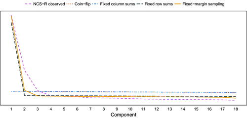
By sampling datasets in which only the row- and column-totals are fixed to be identical to the original data, Steinley et al. (2017) do not sample random data as intended. Rather, they sample data under a unidimensional Rasch model (Verhelst, 2008). To illustrate this, we sampled 1,000 random datasets with margins constrained to be the same as the margins of the dataset evaluated by Steinley et al. (2017): the NCS-R dataset (Kessler et al., 2003). We followed the fixed-margin sampling procedure described by Steinley et al. (2017), generating datasets using the supplementary Matlab codes from Miller & Harrison (2013),² which Steinley et al. (2017) cite as the source of their methodology, and constructing the 99% intervals for each edge-weight by taking the 5th and 995th ordered value. The 99% intervals of the eigenvalues of the Pearson product moment correlation matrix derived from this fixed-margin sampling procedure are shown in Figure 1. For comparison, we also included (a) the eigenvalues of the original NCS-R dataset, (b) the 99% intervals of eigenvalues based on coin-flip random data (every cell is 1 with 50% probability), (c) random data with the same row-sums as the NCS-R, and (d) random data with the same column-subs as the NCS-R. As Figure 1 makes clear, fixed-margin sampling (as well as keeping only the row sums fixed) leads to overt unidimensionality, which strongly deviates from the definition of randomness typically taken in psychology and psychometrics. Keeping the column-sums fixed, in contrast to keeping both column- and row-sums fixed, has little to no effect on the correlational structure. Of note, if one should take such strong unidimensionality as a definition of randomness, then results obtained with every model that assumes unidimensionality (e.g., factor models) should be re-evaluated and will likely be classified as uninteresting.

Figure 1. Scree-plot of eigenvalues based on (black) the NCS-R dataset, (blue) sampling random binary datasets with the same margins as the NCS-R, (red) sampling random binary datasets with the same column sums as the NCS-R, (purple) sampling random binary datasets with the same row sums as NCS-R, and (green) random coin-flip data. The green “coin-flip” area is near invisible as it is near identical to the red “fixed column sums” area.

The Rasch model and the Ising model

The Rasch model is statistically equivalent to a specific type of Ising model: the Curie-Weiss model as shown in Figure 2 (Epskamp, Maris, Waldorp, & Borsboom, 2018; Kruis & Maris, 2016; Marsman et al., 2018; Marsman, Maris, Bechger, & Glas, 2015). As such, generating data under a Rasch model is identical to generating data under a Curie-Weiss model. Therefore, when generating random data while keeping margins constrained, the expected network model is a fully connected network with roughly the same edge weights (Epskamp, Kruis, & Marsman, 2017). As factor models typically perform adequately on psychological data, the expected network structures likely feature many clusters of items intended to measure a latent trait. In fact, the equivalence between network models and factor models was an important part of the reasoning behind the use of network models: a model of direct interactions may lead to data indistinguishable from a general factor model (Van Der Maas et al., 2006). As such, it is not surprising that many edges are not different from what is to be expected in fixed-margin sampling, especially when applied to variables designed to measure a single or multiple highly correlated latent variables. We would therefore not expect networks to show many results Steinley et al. (2017) would deem (potentially) interesting.

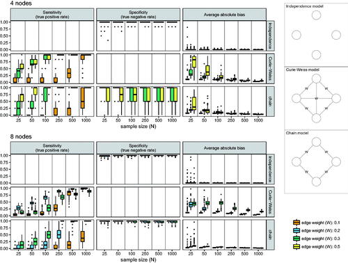
Figure 2. Results from simulation study 1 assessing the performance of eLasso Ising model estimation (left) and models under which data were simulated (right).

How does the fixed-margin test work?

The fixed-margin sampling procedure gives rise to such strong unidimensionality because the sum-scores of people do not behave as would be expected due to chance. Many people have no symptoms at all, and some people have many symptoms. This distribution of the sum-score is not a nuisance parameter that should be controlled for in psychological research akin to the commonness of birds. In fact, the entire field of psychopathology aims to explain why symptoms co-occur and why some people have a high sum-score on symptom inventories. As such, sampling random datasets while keeping margins constrained both induces unidimensionality and takes away the very thing we aim to explain. So, what does the fixed-margin sampling actually test? Verhelst (2008) is very clear on that: the method tests “if the Rasch model is valid” (p. 705), which we can equivalently state as “if the Curie-Weiss model is valid.” When the Curie-Weiss model is the true generating model, we would thus not expect the fixed-margin sampling to classify any result as (potentially) interesting.

Networks of entities and networks of random variables

To understand why fixed-margin sampling is a useful technique in some areas of network science, but has limited utility for network psychometrics, it is important to discuss the difference between such psychometric models and other networks commonly constructed in network science (e.g., social or railroad networks; Newman, 2010). The crux of the matter lies in that a psychometric network is not a network of entities, but rather a network of random variables. This section will discuss the difference between these types of networks.

Suppose we are interested in relationships between actors. We can form a data-matrix with columns indicating actors, rows indicating movies, and a 1 (0) indicating an actor played (did not play) in a movie: We can use this data to construct an actor–movie network of actors and movies in which an edge connects an actor to a movie when that actor played a role in that movie: $$\text{Inception}\hspace{0.17em}–\hspace{0.17em}\text{Leonardo} \text{DiCaprio}\hspace{0.17em}–\hspace{0.17em}\text{Titanic}\hspace{0.17em}–\hspace{0.17em}\text{Kate}\hspace{0.17em}\text{Winslet}$$ Such a network can be termed a two-mode network (bipartite graph; Steinley et al., 2017), as the nodes consist of two sets of entities: movies and actors. Note that movies and actors are not random variables, as they do not take on multiple states, such as “on” or “off.” Rather, it is the edge that can be “present” or “absent.” Furthermore, the connections are observed and typically serve as the dependent variables in a network study. Fixed-margin sampling provides an adequate null distribution for the absence or presence of such ties, given that some actors play in many movies and some movies feature many actors. In addition, one could take a natural projection of the two-mode network into a one-node network. Consider, for example, the actor–actor network: $$\text{Leonardo} \text{DiCaprio} – \text{Kate} \text{Winslet}$$ The connection between the two actors is directly observable as both actors share a movie (Titanic), as can be seen from the two-mode network. Likewise, a movie–movie projection could be formed: $$\text{Inception} – \text{Titanic}$$ Again, fixed-margin sampling provides an adequate null distribution for parameters of these networks, as both one-mode networks are directly derived from the two-mode actor-movie network. If we were to include several movies with a large ensemble cast of actors, we would expect many links in the actor–actor network by chance given the properties of the two-mode network. Similarly, if we would include several actors who played in many movies, we would expect links in the movie–movie network by virtue of the same properties of the two-mode network.

Now consider a symptom-presence data matrix, with rows indicating people, columns indicating symptoms, and a 1 (0) indicating the presence (absence) of a symptom: Then, it is not sensible to encode this data as a two-mode network of entities: $$\text{Depressed} \text{mood} – \text{Bob} – \text{Fatigue} – \text{Alice}$$ It is not sensible because “fatigue” is not an entity in the world that interacts with both Bob and Alice. Likewise, the symptoms present in Bob are not likely to affect the symptoms present in Alice, assuming Bob and Alice do not know each other.³ We could take the one-mode projection to form a person–person network: $$\text{Bob} – \text{Alice}$$ But this network makes no sense, as Bob and Alice do not interact with one-another because they both have fatigue. Likewise, we could form the one-mode symptom-symptom network: $$\text{Depressed} \text{mood} – \text{Fatigue}$$ But again, it is questionable if this network makes sense, given that, in this dataset, the presence of fatigue is independent of the presence of depressed mood (in fact, in the example above, depressed mood has no variance).

Table

	Leonardo DiCaprio	Kate Winslet
Titanic	1	1
Inception	1	0

Table

	Depressed mood	Fatigue
Bob	1	1
Alice	1	0

Instead of symptoms being entities, Bob and Alice have their own set of symptoms, which can be either present (1) or absent (0). The nodes thus represent random variables, and not entities. Such networks of random variables aim to explain why certain realizations of one variable (e.g., a person suffering from depressed mood) co-occur with realizations of another variable (e.g., the same person suffering from fatigue). Edges between the nodes represent some statistical relationship, such as a (partial) correlation, that cannot directly be observed but needs to be estimated from data (Epskamp, Borsboom, & Fried, 2018), and that, by using vetted methods (Borsboom, Robinaugh, Psychosystems Group, Rhemtulla, & Cramer, 2018), come close to some “true” network model. The interest in studying networks of random variables is not to study the relationships between entities, but rather to explain the likelihood of different states that may occur, and why some variables tend to be in the same state. The actor–actor network does not aim to explain why some movies contain many actors, but the symptom network does aim to explain why some people endorse many symptoms (i.e., why they develop psychopathology; Cramer et al., 2016).

In sum, binary data matrices as typically used in (network) psychometrics should not be interpreted as two-mode networks, as the columns and rows do not represent different sets of entities but rather random variables and independent realizations respectively. While fixed-margin sampling adequately controls for the total number of connections (degree) of each node in the two-mode networks of entities, it introduces strong structure in the data-matrix used to estimate networks of random variables, as it conditions on one of the most important things the network of variables aims to explain: the number of present variables. As the data-matrix should not be interpreted as a two-mode network, the derived psychometric networks should also not be interpreted as one-mode projections. This, however, is exactly the way in which Steinley et al. (2017) interpret the data matrix as well as the Ising model (p. 1008):

“Generally, there are two types of networks that can be considered: (1) networks that directly assess the relationships between the same set of observations (e.g., one-mode matrices as described above), and (2) affiliation networks where the connections are assessed between two sets of observations (two-mode matrices as described above). Clearly, psychopathology networks fall into the class of affiliation matrices where the connections are measured between observation and diagnostic criteria. The relationships between the criteria are then then derived by transforming the two-mode affiliation matrix to a one-mode so-called ‘overlap/similarity’ matrix between the criteria, where traditional network methods are applied to this overlap/similarity matrix.”

Simulation studies

As argued above, fixed-margin sampling induces strong unidimensionality. Combining fixed-margin sampling with eLasso Ising model estimation should therefore be interpreted as a method for assessing the performance of the Rasch model, not general Ising models. To showcase this, we performed three simulation studies. In the first study, we generated data under three types of Ising models and assessed the performance of eLasso in retrieving the network structure as well as fixed-margin sampling in correctly classifying true (false) effects as interesting (uninteresting). In the second study, we investigated the performance of fixed-margin sampling coupled with eLasso estimation in multi-dimensional departures from the Rasch model. Finally, in the third study, we investigated the performance of fixed-margin sampling coupled with eLasso estimation in departures from the Rasch model in discrimination of indicators. The results of these studies are described below.

Simulation study 1: Performance of eLasso and fixed-margin sampling in Ising models

We simulated data under three of the simplest forms of the Ising model (Figure 2): an independence model (left panel) in which four binary variables were simulated at random (all edge parameters are zero), a Curie-Weiss model (Kac, 1968) in which all edge parameters are of the same (non-zero) strength (middle panel),⁴ and a chain model (right panel), in which some edges are zero and some edges are non-zero. Simulating data under such true models has the advantage that we now know exactly when an estimated parameter is in the true model and when it arose due to chance. Table 1 shows an overview of possible outcomes in the estimation procedure: an edge can either be present or absent in the true model, and correctly identified as such (true positive and true negative respectively), or incorrectly identified to be present when absent (false positive/Type I error) or absent when present (false negative/Type II error). False positives indicate edges that are detected due to chance. For the independence model, any edge in the estimated network arose due to chance. For the chain model, any edge in the estimated network that is zero in the true model arose due to chance. As a result, these simulations allow us to evaluate both eLasso and fixed-margin sampling approaches and their ability to identify genuine edges in the network.

Common metrics to evaluate the performance of an estimation procedure are the sensitivity, specificity, and, bias (Epskamp & Fried, 2018; van Borkulo et al., 2014). The sensitivity, also known as the true positive rate, indicates the proportion of true edges that were also estimated: $$\text{sensitivity}=\mathrm{ }\frac{\#\text{true positives}}{\#\text{true positives}+\#\text{false negatives}}.$$ The specificity, also known as the true negative rate, indicates the proportion of true absent edges that were also estimated as being absent: $$\text{specificity}=\mathrm{ }\frac{\#\text{true negatives}}{\#\text{true negatives}+\#\text{false positives}}.$$ Finally, the bias indicates the average absolute deviation from the true and estimated parameters: $$\text{bias}=\mathrm{ }\frac{1}{\#\text{parameters}} \sum |\text{true parameter}-\text{estimated parameter}|.$$ Ideally, sensitivity should increase with larger sample sizes (indicating an increase in statistical power), specificity should be high all-around (indicating that few edges are detected due to chance) and bias should decrease with larger sample sizes (indicating that parameters converge to the true values). Each cell of Table 1 can be classified as (potentially) interesting or uninteresting, leading to eight possible outcomes for each parameter in a simulation study. To evaluate the performance of fixed-margin sampling, we propose to assess how often this method classifies true effects as (potentially) interesting and false effects as uninteresting. We graphically display all possible outcomes below.

We simulated data of four variables under the following simplified form of the Ising model (Epskamp, Maris, Waldorp, & Borsboom, 2018): $$P\left(\mathit{x}\right)=\mathrm{ }\frac{1}{Z}\exp \left(\frac{1}{2}\mathrm{ }{\mathit{x}}^T\mathbf{\Omega }\mathrm{ }\mathit{x}\right),$$ in which x denotes a vector of observed dichotomous variables,⁵ encoded with −1 or 1, Z denotes a normalizing constant, and $\mathbf{\Omega }$ encodes the network structure. The Ising model typically also includes a threshold vector (intercepts), which we set to 0 here, leading to a base-rate of 50% chance on a 1 and 50% chance on a −1 for all variables. To obtain the 4-node models shown in Figure 2, we can set the network structure for the independence model as follows: $$\mathbf{\Omega }=\left[\begin{array}{cccc}0& 0& 0& 0\\ 0& 0& 0& 0\\ 0& 0& 0& 0\\ 0& 0& 0& 0\end{array}\right],$$ the Curie-Weiss model as follows: $$\mathbf{\Omega }=\left[\begin{array}{cccc}0& W& W& W\\ W& 0& W& W\\ W& W& 0& W\\ W& W& W& 0\end{array}\right],$$ And finally, the chain model as follows: $$\mathbf{\Omega }=\left[\begin{array}{cccc}0& W& 0& W\\ W& 0& W& 0\\ 0& W& 0& W\\ W& 0& W& 0\end{array}\right].$$ We used the same method for generating data in all models. Data were generated with the IsingSampler package for R, using the Coupling from the Past algorithm (Murray, 2007; Propp & Wilson, 1996), a variant of the Metropolis-Hastings algorithm in which convergence is guaranteed. We varied the number of nodes from 4 to 8. In the 4-node networks, edge-weight (W) varied between 0.1, 0.3, and 0.5. In the 8-node networks, edge-weight (W) varied between 0.1, 0.2, and 0.3, as the W = 0.3 variant of the Curie-Weiss model already led to most sampled cases either endorsing (scored 1) or not endorsing (scored −1) all items, and higher edge-weights lead to convergence problems in generating data. We generated data using a sample size (N) of 25, 50, 100, 250, 500, and 1,000 and repeated every condition 100 times. This led to 3 (condition) × 2 (# nodes) × 3 (W) × 6 (N) × 100 = 10,800 simulated datasets. We performed eLasso using the default settings of the IsingFit package for R. Next, we implemented the fixed-margin sampling as described by Steinley et al. (2017).

Results

The main results of the simulations study are shown in Figure 2 (showing the performance of eLasso network estimation) and Figure 3 (showing the performance of fixed-margin sampling). Figure 2 shows that eLasso adequately retrieves the true network structure: specificity of eLasso was high all-around, indicating that eLasso rarely wrongly estimates an edge due to chance alone. Sensitivity increases with sample size, indicating that with higher power more true edges are detected. The bias in estimated network structures is low and decreases with sample-size, although it should be noted that in the independence model this is aided by LASSO regularization putting edges exactly at 0. The simulations indicate that eLasso converges to the true models: with increasing sample-size, sensitivity becomes higher and bias lower. This is expected behavior: eLasso, akin to significance testing, cannot distinguish between a true null hypothesis and noisy data (Epskamp & Fried, 2018). As a result, with small sample sizes, eLasso will err on the side of caution and set edges to zero in the case of limited evidence that an edge is non-zero.

Figure 3. Results from simulation study 1 assessing the performance of fixed-margin sampling. The areas indicate the proportion of every possible outcome. Outcomes indicating good performance are placed on the bottom, and outcomes indicating poor performance are placed on the top. The horizontal black lines indicate the sum of all outcomes indicating good performance.

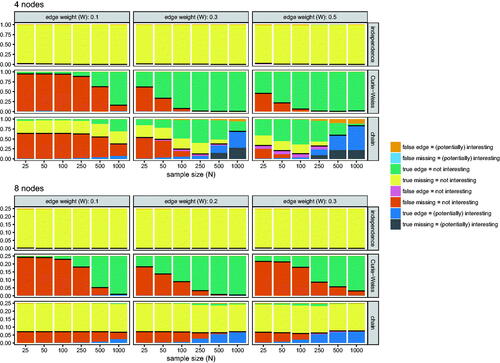
Figure 3 shows the performance of fixed-margin sampling in classifying true and false effects as (potentially) interesting and uninteresting respectively. Given the above theoretical description of the equivalence between Rasch and Curie-Weiss models, “classified as (potentially) interesting” should be interpreted as “is not to be expected given a Curie-Weiss or Rasch model.” As anticipated, fixed-margin sampling shows very poor performance in the Curie-Weiss model and the independence model (a special case of Curie-Weiss model). Regardless of the sample size, the correctly identified present (Curie-Weiss) or absent (independence) edges are not identified as being (potentially) interesting. At lower sample-sizes, fixed-margin sampling correctly classifies false missing edges in the Curie-Weiss model (due to lack of power) as uninteresting. Also as expected, performance of fixed-margin sampling was better in the chain model. In the 4-node simulation, fixed-margin sampling correctly classified most true effects as (potentially) interesting, although it required a relatively high sample size (N > 500 with four variables) to attain this precision. In the 8-node network, fixed-margin sampling correctly classified true edges as (potentially) interesting at high sample-size, but incorrectly classified true missings as uninteresting. It should be noted here that the 8-node chain model is much sparser (higher proportion of edge-weights set to 0) than the 4-node chain-model. In conclusion, while eLasso performs well in estimating the true network structure, and rarely estimates an edge due to chance alone (false positive), fixed-margin sampling performs very poorly to moderately in classifying true and false effects as (potentially) interesting and uninteresting respectively.

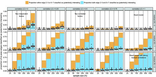
Simulation study 2: Multidimensional departures from the Rasch model

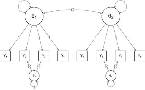
In this second simulation study, we investigated the utility of fixed-margin sampling coupled with eLasso Ising model estimation in datasets generated from multidimensional departures from the Rasch model. We generated data using the multidimensional IRT (MIRT; Reckase, 2009) model shown in Figure 4. The MIRT model models the probability distribution of a set of binary encoded (0 or 1) observed variables ($\mathit{y})$ given a set of latent variables ($\mathit{\theta })$. We denote the observed variables vector with $\mathit{y}$ as it is encoded with 0 and 1 rather than −1 and 1 commonly used in Ising modeling and used above. ⁶ The MIRT model then is: $$P\left(\mathit{y}\mathrm{ }|\mathrm{ }\mathit{\theta }\right)=\prod _{\mathrm{i}}\frac{\text{exp}\left({\mathit{\alpha }}_{\mathbf{i}}^{\mathrm{\prime }}\mathit{\theta }-{\delta }_{\mathbf{i}}\right)}{1+\text{ exp}\left({\mathit{\alpha }}_{\mathbf{i}}^{\mathrm{\prime }}\mathit{\theta }-{\delta }_{\mathbf{i}}\right)},$$ in which ${\delta }_{\mathbf{i}}$ indicates the difficulty of the ith item and ${\mathit{\alpha }}_{\mathbf{i}}^{}$ indicates the ith row of a discrimination matrix A, which is comparable to a factor-loading matrix in factor analysis. In this simulation model, we generated latent variables $\mathit{\theta }$ from a multivariate normal distribution with means of 0 and the following variance–covariance matrix: $$\text{var}\left(\mathit{\theta }\right)=\left[\begin{array}{cccc}1& C& 0& 0\\ C& 1& 0& 0\\ 0& 0& 1& 0\\ 0& 0& 0& 1\end{array}\right],$$ which indicates that the first two factors are correlated at ρ = C, and the last two factors are independent. We varied C between 0, 0.25, 0.5, 0.75, and 1. Next, we specified the discrimination matrix to be: $$\mathit{A}=\left[\begin{array}{cccc}1& 0& 0& 0\\ 1& 0& R& 0\\ 1& 0& R& 0\\ 1& 0& 0& 0\\ 0& 1& 0& 0\\ 0& 1& 0& R\\ 0& 1& 0& R\\ 0& 1& 0& 0\end{array}\right],$$ in which R corresponds to the strength of the residual covariance, which we varied between 0 (no residual correlation), 1 (as much covariance due to the residual factor as due to the main factor) and 2 (more covariance due to the residual factor than due to the main factor). Finally, we drew the difficulty parameters from standard normal distributions. Of note, in the special case of C = 1 and R = 0, the MIRT model above reduces to a Rasch model. Thus, the simulation was set up to depart from Rasch models in two ways: multi-dimensionality (C) and residual correlations (R). Multidimensionality can be seen as a global departure from the Rasch model, because it affects the correlations among all variables, whereas residual correlations can be seen as a local departure, because they affect single pairs of variables (i.e., variables 2 and 3, and 6 and 7). We varied N again between 25, 50, 100, 250, 500, and 1,000. Every condition was replicated 100 times, leading to 5 (C) × 3 (R) × 6 (N) × 100 = 9,000 generated datasets.

Figure 4. Simulation setup for the second simulation study. The generated model is a multidimensional item-response model, in which the correlation between two main factors was varied as well as the strength of two residual correlations.

Results

Figure 5 shows the results of the second simulation study. As expected, in the special case of the Rasch model (C = 1 and R = 0) almost no edges were classified as (potentially) interesting. Departing from the Rasch model by both varying the factor correlation or the strength of residuals leads to more edges being classified as (potentially) interesting. However, it is of note that even at N = 1,000 only a moderate proportion of the edges was classified as (potentially) interesting, even when two uncorrelated factors were simulated. Of note, when simulating two uncorrelated factors with no residual correlation (C = 0 and R = 0), edges between indicators of the same factor were classified as interesting more often than edges between the two factors.⁷ When the magnitudes of the residuals were increased, the two relevant edges (2–3 and 6–7) were classified to be (potentially) interesting with high probability. Because varying C structurally changes the entire model for all variables to be completely different from the Rasch model (when C = 0 two independent factors cause the item responses), and R only leads to deviations in specific parts of the model (two residual correlations), the results indicate that fixed-margin sampling coupled with eLasso Ising model estimation performed very well in detecting local departures from the Rasch model, but is only moderately capable of detecting global departures from the Rasch model. Of note, the dataset analyzed by Steinley et al. (2017) consisted of indicators of two disorders. These simulations suggest we should not expect many edges to be classified as (potentially) interesting in such a case even though the model is not a Rasch model. This is in line with the findings of Steinley et al. (2017).

Figure 5. Results from the second simulation studies. The box-plots indicate the proportion of edges that were classified as (potentially) interesting, with the dashed line indicating the proportion of the two pairs of interest (2–3 and 6–7) compared to all possible edges (8 × 7/2 = 28). The bars in the background indicate the proportion either one (blue + orange area) or both (blue area) the edges of interest were classified as (potentially) interesting.

Simulation study 3: Interchangeability of indicators

The Rasch model dictates both unidimensionality and interchangeability of indicators. Where the second simulation study investigated multidimensional departures from the Rasch model, the third simulation study was set up to investigate departures in interchangeability from the Rasch model. The two-parameter logistic model, (2PL) also known as the Birnbaum model (Birnbaum, 1968), generalizes the Rasch model to incorporate that some items are better indicators of the latent factor than other items (these items are said to discriminate better). We simulated data under a unidimensional 2PL model as shown in Figure 6 by specifying: $$\mathit{A}=\left[\begin{array}{c}1-3D\\ 1-2D\\ 1-D\\ 1\\ 1+D\\ 1+2D\\ 1+3D\end{array}\right].$$

Figure 6. Simulation setup for the third simulation study. The generated model is a unidimensional item-response model known as the two-parameter logistic model or Birnbaum model (Birnbaum, 1968). When D = 0, the model reduces to a Rasch model.

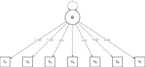
If D = 0, all discrimination parameters are equal and thus the 2PL reduces to the Rasch model. If D > 0, the seventh item will discriminate best and the first item will discriminate worst. We varied D between 0, 0.1, 0.2, and 0.3. The (single) latent variable and the difficulty parameters were all generated from standard normal distributions. N was again varied between 25, 50, 100, 250, 500, and 1,000, and each condition was again replicated 100 times. In total, 4 (D) × 6 (N) × 100 = 2,400 datasets were generated.

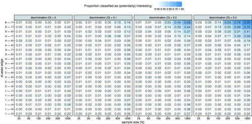
Results

Figure 7 shows the results of the third simulation study. As expected, when D = 0 (Rasch model), hardly any edges (1.1% over all conditions) were classified as (potentially) interesting. When discrimination increased, only edges between indicators with strong discrimination parameters were classified as (potentially) interesting, and only in large samples. The edge between the two most important indicators, Y₆ and Y₇ was classified to be (potentially) interesting in 95% of the N = 1,000 datasets. In lower sample sizes, even when there were strong differences in discrimination fixed-margin sampling coupled with eLasso Ising model estimation did not identify many edges to be (potentially) interesting. As such, the results from the third simulation study are in line with the results from the second simulation study: fixed-margin sampling coupled with eLasso Ising model estimation may be useful in identifying local departures from the Rasch model (strongly discriminating indicators), but not global departures from the Rasch model (when a 2PL model generated the data, many edges were still not classified as interesting).

Figure 7. Results of the third simulation study. Each row indicates one of the potential edges in the estimated eLasso Ising model, and box color and label indicate the proportion of times the edge was classified as (potentially) interesting.

Discussion

We evaluated the utility of fixed-margin sampling (as proposed by Steinley et al. 2017) for drawing inference from eLasso Ising models (van Borkulo et al., 2014) using both psychometric literature and simulation studies. Both indicate that fixed-margin sampling results in datasets which are indistinguishable from what is generated under a Rasch model, and, thus, also indistinguishable from what is generated under a Curie-Weiss model (an Ising model in which all edges are identical). Consistent with prior work (Barber & Drton, 2015; van Borkulo et al., 2014), we showed that the eLasso performed well in estimating Ising models: few edges were detected due to chance alone and, with increasing sample size, parameter estimates converged on the true values and all edges were detected. In contrast, fixed-margin sampling performed poorly in classifying true effects as (potentially) interesting, demonstrating that this test is not a suitable test for the purpose Steinley et al. (2017) proposed. In addition, we investigate the potency of fixed-margin sampling coupled with eLasso Ising models to detect departures from Rasch (or, equivalently, Curie-Weiss) models. Results indicated that fixed-margin sampling performs well in identifying local departures from the Rasch model (strong residual correlations or strongly discriminating indicators), but lacked statistical power to detect global departures from the Rasch model (many parameters were not classified as interesting even if the data were generated by two independent factors or a factor-model in which indicators were not interchangeable). Overall, these results indicate that the conclusion reached by Steinley et al. (2017), that “many of the [eLasso] results are indistinguishable from what would be expected by chance” (p. 1000), is unwarranted.

The utility of fixed-margin sampling

While fixed-margin sampling is sensible in the analysis of two-mode networks between sets of entities, as discussed above, it may not readily be utilized to assess the performance of regularized Ising models or other multivariate statistical models based on datasets in which columns represent random variables and rows represent independent samples from some distribution. As the implied null-model is a Rasch model, however, the method does show great potency in assessing how well a Rasch model can describe the data (Verhelst, 2008). In this context, fixed-margin sampling is then interpreted as a non-parametric test for the Rach model. Combining fixed-margin sampling with Ising model estimation as proposed by Steinley et al. (2017), may be very interesting, especially in the context of abnormal psychology, as the disease model used in the DSM implicitly assumes a Rasch model (symptoms as interchangeable indicators of an underlying disorder). Combining fixed-margin sampling with Ising model estimation not only allows one to test this hypothesis, but also to see where the Rasch model misfits, without having to estimate Rasch parameters. Our simulations indicated that fixed-margin sampling performed adequately in identifying where misfit of the Rasch model occurs. While fixed-margin sampling therefore provides a useful null-distribution to test where the Rasch model misfits, it does not provide a useful null-distribution to assess if Ising model (of which the Rasch model is a special case) parameters are due to chance.

Is unidimensionality an appropriate null-distribution in network psychometrics?

As network psychometrics has started as an alternative to latent variable modeling, one might argue that taking a Rasch model as null-distribution is sensible. As discussed, however, the Rasch model is not distinguishable from certain Ising models (i.e., Curie-Weiss models). As such, when taking the Rasch model as a null-hypothesis, a failure to reject the null model (Rasch) does not imply the Rasch model to be true. Because of model equivalences, a Curie-Weiss model may still underlie the data. Fixed-margin sampling may have utility in seeing where a Rasch model or Curie-Weiss model does not explain the data, but it does not have utility in evaluating whether an Ising model is the underlying data-generating model. Residual network models are currently being developed that allow researchers to study the network structure beyond the influence of a latent variable (Chen, Li, Liu, & Ying, 2016; Epskamp, Rhemtulla, & Borsboom, 2017).

Of note, when using unidimensionality with interchangeable indicators as null-distribution, our simulations indicate that one should not expect many edges to be classified as (potentially) interesting when the Rasch model is not true. Even when generating two independent factors, only a moderate number of edges were classified as (potentially) interesting.⁸ In this light, the number of 65% of the edges classified as (potentially) interesting reported by Steinley et al. (2017) is fairly high and indicates that their analyzed dataset strongly deviates from what is to be expected given a Rasch or Curie-Weiss model. This makes sense, as the analyzed dataset contains indicators of two disorders, not one, and is further highly influenced by the zero-imputation strategy used to overcome the skip-structure of the data-administration (Borsboom et al., 2017). As such, when applying fixed-margin sampling to assess unidimensionality, it is best to analyze a dataset in which unidimensionality is plausible (e.g., indicators of only one disorder).

Conclusions

While fixed-margin sampling is a promising method for analyzing two-mode networks between entities (e.g., bird–habitat or actor–movie networks), care should be taken when using fixed-margin sampling to evaluate networks of random variables aimed to explain observed states of random variables, such as the Ising model. Our evaluation shows that the fixed-margin sampling cannot readily be used to assess if edges in the Ising model are due to chance, as the implied null-model, a unidimensional factor model with interchangeable indicators, is inappropriate. Instead, applying fixed-margin sampling in combination with Ising models should be used as a method for highlighting local violations of such factor models.

Article information

Conflict of interest disclosures: Each author signed a form for disclosure of potential conflicts of interest. No authors reported any financial or other conflicts of interest in relation to the work described.

Ethical principles: The authors affirm having followed professional ethical guidelines in preparing this work. These guidelines include obtaining informed consent from human participants, maintaining ethical treatment and respect for the rights of human or animal participants, and ensuring the privacy of participants and their data, such as ensuring that individual participants cannot be identified in reported results or from publicly available original or archival data.

Funding: Claudia van Borkulo was supported by ERC Consolidator Grant no. 647209, Don Robinaugh was supported by European Research Council Consolidator Grant no. 647209 and Angelique Cramer was supported by NWO Veni grant no. 451-14-002. All other authors were not supported by grants at the time of writing.

Role of the funders/sponsors: None of the funders or sponsors of this research had any role in the design and conduct of the study; collection, management, analysis, and interpretation of data; preparation, review, or approval of the manuscript; or decision to submit the manuscript for publication.

Acknowledgments: The ideas and opinions expressed herein are those of the authors alone, and endorsement by the authors’ institutions or funding agencies is not intended and should not be inferred.

Notes

1 Steinley et al. (2017) term these intervals confidence intervals. We have opted to avoid this terminology as the term x% confidence interval is commonly used to denote an interval in which x% of intervals constructed in such fashion should contain the true parameter of interest. The Steinley et al. (2017) method does not construct such confidence intervals, which are still a topic of future research for centrality indices in particular (Epskamp et al., 2017).

2 http://jwmi.github.io/software.html

3 It is typical to assume independence of cases in many statistical analyses.

4 Of note, eLasso is not the most appropriate method to estimate Curie-Weiss models, as it assumes and searches for a model that is sparse (contains missing edges; Epskamp et al., 2017). The Curie-Weiss model is better estimable using the methodology of Marsman et al. (2015), which we did not evaluate here as it was not mentioned by Steinley et al. (2017).

5 We chose to generate data encoded with −1 and 1 because it is more common in Ising modeling, it simplifies the matrix Ising model expression, and allows the threshold vector to be fixed at 0 for 50% base-rates. The Ising model matrix based on data encoded with −1 and 1 is proportional to the matrix encoding the Ising model corresponding to data encoded with 0 and 1 (zeroes remain zeroes in both cases). As such, the choice is arbitrary. In the simulation study, we transformed the results from eLasso (which uses 0 and 1) to results based on an −1 and 1 encoding.

6 We use 0 and 1 encoding here because it is more common in MIRT, as well as simplifies the expression. Note, again, that the encoding is arbitrary for the Ising network structure, and a network obtained under one encoding can be transformed to a network obtained under a different encoding.

7 Closer inspection of the generated Ising models revealed that the Ising models estimated from data in the C = 0 and R = 0 condition generally formed two fully connected clusters (indicators of each factor clustering together), with little to no connections between the clusters. Ising models estimated from the fixed-margin samples in this condition were mostly very sparse and only contained a few connections. As such, while edges in the two clusters featured adequate probability of being classified as (potentially) interesting, most estimated missing edges were classified as uninteresting.

8 It is possible that LASSO regularization itself influences these results. LASSO regularization pushes many parameters, both in the original data and in the fixed-margin samples, to zero (Epskamp, Kruis, & Marsman, 2017), leading to both observed parameters and one or both interval boundaries based on the fixed-margin samples to be exactly zero. It is possible that unregularized Ising model estimation performs better, but this investigation was beyond the scope of this article, and unregularized Ising model estimation is not trivial (Epskamp et al., in press).

References

- Agresti, A. (1990). Categorical data analysis. New York, NY: Wiley.
- Barber, R. F., & Drton, M. (2015). High-dimensional Ising model selection with Bayesian information criteria. Electronic Journal of Statistics, 9(1), 567–607.
- Birnbaum, A. (1968). Some latent trait models and their use in inferring an examinee’s ability. In F. Lord & M. Novick (Eds.), Statistical theories of mental test scores. (pp. 397–479) Reading, MA: Addison-Wesley.
- Borsboom, D., Fried, E., Epskamp, S., Waldorp, L., Van Borkulo, C., Van Der Maas, H.,…Cramer, A. (2017). False alarm? A comprehensive reanalysis of “Evidence that psychopathology symptom networks have limited replicability” by Forbes, Wright, Markon, and Krueger. Journal of Abnormal Psychology, 126(7), 989–999. https://doi.org/10.17605/OSF.IO/TGEZ8
- Borsboom, D., Robinaugh, D. J., Psychosystems Group, Rhemtulla, M., & Cramer, A. O. (2018). Robustness and replicability of psychopathology networks. World Psychiatry. 17(2), 143–144. https://doi.org/10.1002/wps.20515
- Chen, Y., Li, X., Liu, J., & Ying, Z. (2016). A fused latent and graphical model for multivariate binary data. Retrieved from https://arxiv.org/pdf/1606.08925.pdf
- Connor, E. F., & Simberloff, D. (1979). The assembly of species communities: Chance or competition?. Ecology, 60(6), 1132. https://doi.org/10.2307/1936961
- Cramer, A. O. J., van Borkulo, C. D., Giltay, E. J., van der Maas, H. L. J., Kendler, K. S., Scheffer, M.,…Borsboom, D. (2016). Major depression as a complex dynamic system. Plos One, 11(12), e0167490. https://doi.org/10.1371/journal.pone.0167490
- Epskamp, S., Borsboom, D., & Fried, E., I. (2018). Estimating psychological networks and their accuracy: A tutorial paper. Behavior Research Methods, 50(1), 195–212. https://doi.org/10.3758/s13428-017-0862-1
- Epskamp, S., & Fried, E. I. (2018). A tutorial on regularized partial correlation networks. Psychological Methods.Advance online publication. http://dx.doi.org/10.1037/met0000167
- Epskamp, S., Kruis, J., & Marsman, M. (2017). Estimating psychopathological networks: Be careful what you wish for. PLoS One, 12(6), e0179891. https://doi.org/10.1371/journal.pone.0179891
- Epskamp, S., Maris, G. K. J., Waldorp, L. J., & Borsboom, D. (2018). Network psychometrics. In P. Irwing, T. Booth, & D.J. Hughes (Eds.), Wiley Handbook of Psychometric Testing: A Multidisciplinary Reference on Survey, Scale and Test Development. London: John Wiley & Sons
- Epskamp, S., Rhemtulla, M. T., & Borsboom, D. (2017). Generalized network psychometrics: Combining network and latent variable models. Psychometrika, 82(4), 904–927. https://doi.org/10.1007/s11336-017-9557-x
- Forbes, M. K., Wright, A. G. C., Markon, K. E., & Krueger, R. F. (2017a). Evidence that psychopathology symptom networks have limited replicability. Journal of Abnormal Psychology, 126(7), 969–988. https://doi.org/10.1037/abn0000276
- Forbes, M. K., Wright, A. G. C., Markon, K. E., & Krueger, R. F. (2017b). Further evidence that psychopathology networks have limited replicability and utility: Response to Borsboom et al. and Steinley et al. Journal of Abnormal Psychology, 126(7), 1011–1016.
- Harrison, M. T., & Miller, J. W. (2013). Importance sampling for weighted binary random matrices with specified margins. Retrieved from https://arxiv.org/pdf/1301.3928.pdf
- Hastie, T., Tibshirani, R., & Friedman, J. H. (2001). The elements of statistical learning. New York, NY, USA: Springer New York Inc.
- Hastie, T., Tibshirani, R., & Wainwright, M. J. (2015). Statistical learning with sparsity: The lasso and generalizations. Boca Raton, FL, USA: Taylor & Francis.
- Kac, M. (1968). Mathematical mechanism of phase transition. In M. Chrétien, E. Gross, & S. Deser (Eds.), Statistical physics: Phase transitions and superfluidity, vol. 1, Brandeis university summer institute in theoretical physics (pp. 241–305). New York, NY: Gordon and Breach Science Publishers.
- Kessler, R. C., Berglund, P., Demler, O., Jin, R., Koretz, D., Merikangas, K. R.,…Wang, P. S. (2003). The epidemiology of major depressive disorder. JAMA, 289(23), 3095. https://doi.org/10.1001/jama.289.23.3095
- Kruis, J., & Maris, G. (2016). Three representations of the Ising model. Scientific Reports, 6(1), 34175. https://doi.org/10.1038/srep34175
- Marsman, M., Borsboom, D., Kruis, J., Epskamp, S., van Bork, R., Waldorp, L. J.,…Maris, G. (2018). An introduction to network psychometrics: Relating Ising network models to item response theory models. Multivariate Behavioral Research, 53(1), 15–35. https://doi.org/10.1080/00273171.2017.1379379
- Marsman, M., Maris, G., Bechger, T., & Glas, C. (2015). Bayesian inference for low-rank Ising networks. Scientific Reports, 5(1), 9050–9057.
- Meinshausen, N., & Bühlmann, P. (2006). High-dimensional graphs and variable selection with the lasso. The Annals of Statistics, 34(3), 1436–1462.
- Miller, J. W., & Harrison, M. T. (2013). Exact sampling and counting for fixed-margin matrices. The Annals of Statistics, 41(3), 1569–1592. https://doi.org/10.1214/13-AOS1131
- Murray, I. (2007). Advances in Markov chain Monte Carlo methods. University College London: Gatsby Computational Neuroscience Unit.
- Newman, M. (2010). Networks: An introduction. Oxford, UK: University Press.
- Pearl, J. (2000). Causality: Models, reasoning and inference (Vol.29). Cambridge, UK: Cambridge Univ Press.
- Propp, J. G., & Wilson, D. B. (1996). Exact sampling with coupled Markov chains and applications to statistical mechanics. Random Structures and Algorithms, 9(1-2), 223–252. https://doi.org/10.1002/(SICI)1098-2418(199608/09)9:1/2<223::AID-RSA14>3.0.CO;2-O
- Rasch, G. (1960). Probabilistic models for some intelligence and attainment tests. Copenhagen, DM: Danish Institute for Educational Research.
- Reckase, M. D. (2009). Multidimensional item response theory. New York, NY, USA: Springer.
- Steinley, D., Hoffman, M., Brusco, M. J., & Sher, K. J. (2017). A method for making inferences in network analysis: Comment on Forbes, Wright, Markon, and Krueger (2017). Journal of Abnormal Psychology, 126(7), 1000–1010.
- Tibshirani, R. (1996). Regression shrinkage and selection via the lasso. Journal of the Royal Statistical Society. Series B (Methodological), 58, 267–288.
- van Borkulo, C. D., Borsboom, D., Epskamp, S., Blanken, T. F., Boschloo, L., Schoevers, R. A.,…Waldorp, L. J. (2014). A new method for constructing networks from binary data. Scientific Reports, 4, 5918. Retrieved from http://www.ncbi.nlm.nih.gov/pubmed/25082149%5Cnhttp://www.pubmedcentral.nih.gov/articlerender.fcgi?artid=4118196&tool=pmcentrez&rendertype=abstract
- van Borkulo, C. D., & Epskamp, S. (2014). IsingFit: Fitting Ising models using the eLasso method. Retrieved from http://cran.r-project.org/package=IsingFit
- Van Der Maas, H. L. J., Dolan, C. V., Grasman, R. P. P. P., Wicherts, J. M., Huizenga, H. M., & Raijmakers, M. E. J. (2006). A dynamical model of general intelligence: The positive manifold of intelligence by mutualism. Psychological Review, 113(4), 842–861.
- Verhelst, N. D. (2008). An efficient MCMC algorithm to sample binary matrices with fixed marginals. Psychometrika, 73(4), 705–728. https://doi.org/10.1007/s11336-008-9062-3