The Role of Time in the Quest for Understanding Psychological Mechanisms

Abstract

The lead-lag structure of multivariate time-ordered observations and the possibility to disentangle between-person (BP) from within-person (WP) sources of variance are major assets of longitudinal (panel) data. Hence, psychologists are making increasing use of such data, often with the intent to delineate the dynamic properties of psychological mechanisms, understood as a sequence of causal effects that govern psychological functioning. However, even with longitudinal data, psychological mechanisms are not easily identified. In this article, we show how an adequate representation of time may enhance the tenability of causal interpretations in the context of multivariate longitudinal data analysis. We anchor our considerations with an example that illustrates some of the main problems and questions faced by applied researchers and practitioners. We distinguish between static versus dynamic and discrete versus continuous time modeling approaches and discuss their advantages and disadvantages. We place particular emphasis on different ways of addressing BP differences and stress their dual role as potential confounds versus valuable sources of information for improving estimation and aiding causal inference. We conclude by outlining an approach that offers the potential of better integration of information on BP differences and WP changes in the search for causal mechanisms along with a discussion of current problems and limitations.

Keywords:

• Time
• continuous time
• psychological mechanisms
• between-person versus within-person research
• causality

Introduction

To improve the description, explanation, prediction, and modification of human behavior, an increasing number of researchers resort to longitudinal studies (Hamaker & Wichers, 2017; Hsiao, 2007). This development has been fueled by recent technological advances, such as smartphones or wearable devices (Mehl & Conner, 2012; Trull & Ebner-Priemer, 2013), which make the collection of large amounts of data simpler and more affordable. In addition, longitudinal study designs in psychological research have diversified and include classical panel designs (many individuals observed at a few measurement occasions), intensive longitudinal designs (many measurement occasions), single subject time series, as well as various combinations of cross-sectional and longitudinal data. In turn, data analytic challenges related to irregularly spaced measurement occasions, multivariate constructs, and different sources of between-person (BP) and within-person (WP) variation have become the new norm, rather than the exception.

The COGITO study typifies such complexities. In this study, a large test battery of cognitive and non-cognitive measures was administered to 101 younger and 103 older adults across more than 100 daily 1-hour sessions (Schmiedek, Lövden, & Lindenberger, 2010). In addition, participants underwent comprehensive pre- and post-test measurements. Structural and functional brain measures were also collected for some of the individuals. A subset of the participants also are participants in the German socioeconomic panel study (G-SOEP; Wagner, Frick, & Schupp, 2007), linking their data to one of the longest running panel studies worldwide. Thus, various measures were collected across different individuals and were sampled at different measurement occasions, resulting in different data structures from where WP changes and BP differences are assessed. Although the COGITO study is exceptional in many regards, complex longitudinal study designs of this sort are being used more and more regularly.

The increasing availability of large complex data sets is not unique to psychology. In econometrics, for example, data on stock indices are available that go back well over a century. What makes multivariate research in psychology particularly challenging, however, is that we wish to go beyond simple prediction, seeking to understand the mechanisms that underlie the psychological functioning of human behavior. Apart from being an end in itself, understanding psychological mechanisms can also be an important step toward developing effective interventions. Although it is clear that inferring causal mechanisms from complex multivariate data sets is a true challenge, we also believe that current practice suffers from a number of common problems. The goal of this article is to identify some of these problems and to show how they can be avoided by paying closer attention to the role of time.

To achieve this goal, we first introduce an example, which illustrates some typical questions faced by applied researchers and practitioners. These questions serve to structure the remainder of the article. Second, we distinguish between static versus dynamic and discrete versus continuous time modeling approaches and discuss their advantages and disadvantages in the study of psychological mechanisms. Third, we review different approaches to deal with BP differences, highlighting their dual role as a potential source of confounding as well as a source of information to improve the estimation and causal inference. We conclude by outlining an approach that offers the potential of better integration of information on BP differences and WP changes in the search for causal mechanisms, underlying psychological functioning, along with a discussion of current problems and limitations.

The list of problems and potential solutions discussed in this article is far from complete. Likewise, the article does not replace a solid introduction to the statistical techniques (such as continuous time dynamic modeling) discussed in this work. For this more advanced treatment, we will point the reader to the relevant technical literature and software. The primary purpose of this article is to provide an integrative account of common problems in inferring causal mechanisms in multivariate behavioral research, existing solutions, as well as unresolved issues and future research directions. As such, our article necessarily remains somewhat subjective, reflecting our view of the current state of the art. By providing a comprehensive and non-technical discussion of a broad scope, we hope this paper will prove helpful to applied researchers from various fields in their quest to identify and understand psychological mechanisms.

An illustrative example

As a motivating example, consider a scientist, who is also a practicing clinician, specializing in the treatment of social anxiety. She is responsible for a small group of patients, who are treated with anxiolytic antidepressants. In practice, these are typically selective serotonin reuptake inhibitors (SSRIs), which lower the presynaptic absorption of serotonin and thereby increase serotonin in the synaptic cleft. The exact mechanism of SSRI’s effect is still unknown, and their effectiveness for different groups of patients is still subject to some debate. Available evidence from meta analyses of double-blind, placebo-controlled, randomized clinical trials (RCTs), however, has shown SSRIs to be generally effective in reducing social anxiety (Hedges, Brown, Shwalb, Godfrey, & Larcher, 2006).

Despite her trust in the scientific rigor of the meta-analytic studies, to our scientist a medium-to-strong correlation between serotonin level and social anxiety stands in partial contradiction to personal experiences reported by her patients. Her patients typically report only moderate effects of SSRI dosage on anxiety with some even reporting effects in the opposite direction. For this reason, she decides to conduct her own study, aiming to (a) gain a better understanding of the mechanism underlying the relationship between serotonin and social anxiety and to (b) assess whether the meta-analytic results found in between-group (BP) RCTs can be generalized to her own individual patients so that she can offer better patient-centered advice on the use of SSRIs. To this end, she assesses the serotonin level of N  =  50 patients approximately once a week and asks them to complete a social questionnaire at approximately the same time intervals. After 10 months, she has collected data at up to about 40 measurement occasions from the 50 patients. What statistical model should she use to best understand possible mechanisms?

Upon closer inspection of the data, she realizes that the timing between measurement occasions differs greatly within, as well as across individuals. In fact, none of her patients followed exactly the original assessment protocol of 40 weekly measurement occasions. It is obvious to her that the effect of serotonin on social anxiety is unlikely to be instantaneous, but rather unfolds over time, and thus will differ depending on the time interval between the measurements. How should she best handle the different time intervals in the analysis and interpretation of results?

Although the previous RCTs focused almost exclusively on the effect of serotonin on social anxiety, from her clinical experience she knows that this is unlikely to be a one-way effect: Changes in social anxiety (e.g., due to a change in the environment) will likely also affect the subsequent levels of serotonin. Furthermore, she expects social withdrawal behavior to play an important role in the relationship between social anxiety and serotonin, for example, by mediating the effect of social anxiety on serotonin. This raises the question of how should she model and interpret reciprocal and mediation effects and how are such effects manifested for any given time interval?

Although all of her patients suffer from social anxiety, there are large BP differences in the severity of anxiety as well as the level of serotonin. As a practicing clinician, she takes the perspective that each of her patients is unique. As a scientist, however, she believes that there are general mechanisms that apply to all individuals. Should she ignore BP differences by constraining model parameters to equality across individuals? Should she analyze the data from each patient separately? More generally, how should she best deal with between-person differences in longitudinal panel data analysis?

Finally, she wonders about the implications of her study. What if the results for one of her patients contradict the results of existing BP studies? How can she even compare an effect that is inferred from RCTs, representing cross-sectional data on many individuals, to an effect for one of her patients that is inferred from longitudinal data representing a single individual? If the relationship between serotonin and social anxiety in one of her patients is in the opposite direction from the previous RCT studies, should she treat that patient based on the BP results or based on the findings from her own investigation of this particular patient (or both)? More generally, how can we compare and integrate results based on BP differences and those based on WP changes in our quest for causal mechanisms—or should we?

The role of time in longitudinal data analysis

The example from the previous section highlights the kinds of questions clinically oriented psychological researchers and practitioners may be interested in, and the problems they can face when trying to address them. In the following, we will demonstrate how a deeper appreciation of the role of time can guide our thinking in approaching and answering these questions.

Time in static versus dynamic longitudinal models

To answer the first question (what statistical model should one use to best understand possible mechanisms?), it is helpful to distinguish between two broad classes of longitudinal models: static models and dynamic models. We define a dynamic longitudinal model as a model that accounts for (WP) changes in a system of variables over time as a function of the past. Dynamic models are typically formulated in terms of difference equations or differential equations. In contrast, a static longitudinal model accounts for the state of a system of variables, which is often expressed as a function of time.

To contrast the two types of models, let us consider a linear latent growth curve model, which is a typical static model used in psychological research. In its simplest linear form, it can be written as a regression model as shown in Equation 1(1) $$y_i\left(t\right)={\eta }_0+{\eta }_1\cdot t_i+{\zeta }_i\left(t\right).$$(1) : (1) $$y_i\left(t\right)={\eta }_0+{\eta }_1\cdot t_i+{\zeta }_i\left(t\right).$$(1)

$y_i\left(t\right)$ denotes the value of the continuous dependent variable y for individual i  =  1, …, N at a time point $t\in R$. The intercept is denoted by ${\eta }_0$, the linear slope by ${\eta }_1$, and the error term at time point t is denoted by ${\zeta }_i\left(t\right)$. Often, the intercept and slope are assumed to be random variables, so that an additional subscript i may be added to these two terms. As is apparent in Equation 1(1) $$y_i\left(t\right)={\eta }_0+{\eta }_1\cdot t_i+{\zeta }_i\left(t\right).$$(1) , in this model time serves as an exogenous predictor, which accounts for the time-dependent state of the system (i.e., the dependent variable $y_i\left(t\right)$). If the time point is known, we can predict the state of the system (i.e., the dependent variable). This is different in a dynamic model, where the time point is necessary, but not sufficient, to determine the state of a system. To illustrate, let us consider a change score model or autoregressive (cross-lagged) model, which is a typical example of a dynamic model (e.g., McArdle, 2009). A simple autoregressive model is given in Equation 2(2) $$y_i\left(t\right)=a\cdot y_i(t-\Delta t)+{\zeta }_i\left(t\right),$$(2) (2) $$y_i\left(t\right)=a\cdot y_i(t-\Delta t)+{\zeta }_i\left(t\right),$$(2) with time interval $\Delta t$ typically fixed to one. Subtracting $y_i(t-\Delta t)$ from both sides of Equation 2 (i(2) $$y_i\left(t\right)=a\cdot y_i(t-\Delta t)+{\zeta }_i\left(t\right),$$(2) .e., $y_i\left(t\right)-y_i\left(t-\Delta t\right)=(a-1)\cdot y_i(t-\Delta t)+{\zeta }_i\left(t\right)$) turns the autoregressive model formulation into a mathematically equivalent change score model formulation. From this reformulation, it is readily apparent that this model accounts for changes (i.e., $y_i\left(t\right)-y_i\left(t-\Delta t\right)$) in the state of the system as a function of an initial state $y_i(t-\Delta t)$ and the time $\Delta t$ that has passed. Thus, in contrast to static models, knowledge of the time point t alone is not sufficient for predicting the state of the system (i.e., the dependent variable), and we also need to know something about the past (more generally, we need to know the initial state).

Although the two classes of models are not mutually exclusive¹, they provide a useful classification and it is important to be aware of their relative strengths and limitations. For researchers who are just interested in describing change over time (Baltes & Nesselroade, 1979), static longitudinal models offer a simple way to do so. A causal interpretation of such models is not possible. Things change as time changes, things do not change because time changes. In the words of Baltes, Reese, and Nesselroade (1988) “…although time is inextricably linked to the concept of development, in itself it cannot explain any aspect of developmental change” (p. 108). Thus, when the goal is not only to describe change, but to understand the mechanisms that lead to change, dynamic models are needed. The researcher from our introductory example clearly has this goal, as she wants to better understand the mechanisms underlying the relationship between serotonin and social anxiety. To this end, she would be well-advised to consider a dynamic modeling approach.

Discrete time versus continuous time models

The distinction between discrete time and continuous time models is straightforward: In the former, time is treated as a discrete variable that may only take on values from a countable set, whereas in the latter, time is treated as a continuous variable that may take on infinitely many, uncountable, values.

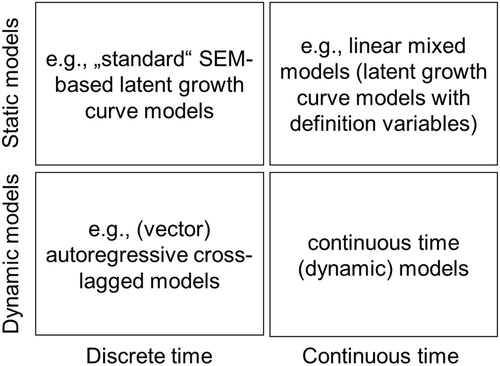
Combined with the previous distinction between static and dynamic models, this second distinction leads to the two-by-two classification of longitudinal models shown in Figure 1. From this classification and the selected examples of prototypical statistical techniques in each cell, we see that treating time as a continuous variable in static models of change is straightforward. Because time is an exogenous predictor (cf. Equation 1(1) $$y_i\left(t\right)={\eta }_0+{\eta }_1\cdot t_i+{\zeta }_i\left(t\right).$$(1) ), it makes little difference whether time is treated as a continuous or discrete variable. The situation is different for dynamic models. When time is treated as a discrete variable, we may compute a change score over a discrete time interval (i.e., $(y_i\left(t\right)-y_i\left(t-\Delta t\right))/\Delta t$) and use discrete time dynamic models such as autoregressive or change score models (cf. Equation 2(2) $$y_i\left(t\right)=a\cdot y_i(t-\Delta t)+{\zeta }_i\left(t\right),$$(2) ). In contrast, when treating time as a continuous variable, differential calculus is needed (described below). The lack of familiarity of applied researchers with differential calculus and the lack of suitable software to implement and estimate such models have severely hampered the use of continuous time dynamic models in modern psychological research.

Figure 1. A two-by-two classification table of longitudinal models: static versus dynamic models (vertical) and discrete versus continuous time models (horizontal) along with selected examples of prototypical statistical techniques in each cell. Given that treating time as a continuous variable in static models of change is straightforward, it is common (although somewhat imprecise) among quantitative researchers to restrict the term “continuous time models” to “continuous time (dynamic) models” (lower right quadrant).

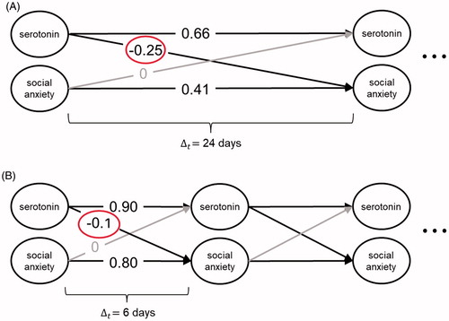
To illustrate why this may be problematic, let us return to the researcher from our example, who has decided to use a dynamic model and has opted for a vector-autoregressive time series model with cross-lagged effects from serotonin to social anxiety. After having estimated the model for two of her patients, she finds herself in the situation illustrated in Figure 2. For one patient (Figure 2A), who was assessed every 24 days, she observed a comparatively strong effect of serotonin on social anxiety, whereas for the second patient (Figure 2B), who was assessed every 6 days, the effect was considerably smaller, despite shorter measurement intervals. How can she determine whether the effects differ because the measurement intervals differ, or because of differences between the two individuals in the linkage between serotonin and social anxiety, possibly indicating different causal mechanisms? The situation is further complicated by the fact that measurement occasions differ not only across, but also within individuals. In order to avoid the problem of potentially biased parameter estimates and effects that cannot be interpreted or compared with one another, it is necessary to better account for the role of time in dynamic longitudinal modeling (cf. Cole & Maxwell, 2003; Gollob & Reichardt, 1987).

Figure 2. Example of a bivariate autoregressive cross-lagged model for estimating the effect of serotonin on social anxiety. (A) Time interval ${\Delta }_t=24$ days between measurement occasions. (B) Time interval ${\Delta }_t=6$ six days between measurement occasions. The effect of social anxiety on serotonin is fixed to zero in both models. The three dots to the right of each panel indicate that in both examples the time series continues until the final measurement occasion.

To demonstrate how this can be achieved, we first consider latent change score models as an established approach to dynamic modeling in psychological research (McArdle, 2009). We then show how the idea underlying latent change score models generalizes to continuous time dynamic models and how the former may be considered a special case of the latter. In line with the goal of this paper, we keep our discussion as non-technical as possible. For a more comprehensive introduction to latent change score models, we refer the reader to work by McArdle, Hamagami, and others (McArdle, 2009; McArdle & Hamagami, 2001, 2004; Kievit et al., 2017). For a step-by-step introduction to continuous time dynamic models in psychology, we refer the reader to work by Oud, Voelkle, and others (Oud & Jansen, 2000; Voelkle, Oud, Davidov, & Schmidt, 2012). For a more technical comparison of the two approaches, see Voelkle and Oud (2015).

Latent change score models

Latent change score models were developed to go beyond the mere description of change offered by static models. For example, McArdle (2009) urged researchers not to start their data analysis by asking “What is your data collection design?” but rather by asking “What is your model for change?” (p. 601) – a sentiment in line with the fundamental idea of dynamic modeling. To this end, he proposed the use of latent change score models (2009, p. 579; McArdle & Hamagami, 2001, 2004). The basic idea of a change score model has already been sketched: Instead of directly predicting the dependent variable at a given point in time, in a change score model we predict the change in a variable over a time interval (i.e., $(y_i\left(t\right)-y_i\left(t-\Delta t\right))/\Delta t=(a-1)\cdot y_i(t-\Delta t)+{\zeta }_i\left(t\right)$). This idea generalizes readily to latent variables and to multivariate models. Instead of y(t), we can use $\mathbf{\eta }\left(t\right)\in R^v$ to denote a vector of $v$ latent variables. Each latent variable may be measured by one or more observed variables via a standard measurement model as is common in structural equation modeling (SEM) (i.e., $\mathbf{y}\left(t\right)=\Lambda \mathbf{\eta }\left(t\right)+\mathbf{\tau }+\mathbf{\epsilon }\left(t\right)$; cf. Bollen, 1989). The vector of latent change variables $\Delta \mathbf{\eta }\left(\Delta t_u\right)$may thus be defined as (3) $$\Delta \mathbf{\eta }\left({\Delta t}_u\right)=\frac{\mathbf{\eta }\left(t_u\right)-\mathbf{\eta }\left(t_{u-1}\right)}{{\Delta t}_u}.$$(3)

The index u denotes the measurement occasion at time point t, highlighting that the difference is always computed between two discrete measurement occasions at $t_u$ and at $t_{u-1}$. In current practice, the time interval is almost always assumed to be $\Delta t_u=1$. With this simplification, the multivariate latent change score formulation of Equation 2(2) $$y_i\left(t\right)=a\cdot y_i(t-\Delta t)+{\zeta }_i\left(t\right),$$(2) can be written as (4) $$\Delta \mathbf{\eta }\left(t_u\right)={\mathbf{A}}^{†}\cdot \mathbf{\eta }\left(t_{u-1}\right)+\mathbf{\zeta }\left(t_u\right),$$(4) with $\mathbf{\zeta }\left(t_u\right)\in R^v$ denoting a vector of $v$ error terms and ${\mathbf{A}}^{†}\in R^{v\times v}$ denoting a $v\times v$ matrix of regression coefficients. The model shown in Equation 4(4) $$\Delta \mathbf{\eta }\left(t_u\right)={\mathbf{A}}^{†}\cdot \mathbf{\eta }\left(t_{u-1}\right)+\mathbf{\zeta }\left(t_u\right),$$(4) is often referred to as a proportional change score model, because change in the vector of dependent variables $\Delta \mathbf{\eta }\left(t_u\right)$ is proportional to the previous level $\mathbf{\eta }\left(t_{u-1}\right)$. That is, future changes increase or decrease proportionally to the level in the past (McArdle & Hamagami, 2004; Voelkle & Oud, 2015).

Note that the dynamic error term $\mathbf{\zeta }\left(t_u\right)$ in Equation 4(4) $$\Delta \mathbf{\eta }\left(t_u\right)={\mathbf{A}}^{†}\cdot \mathbf{\eta }\left(t_{u-1}\right)+\mathbf{\zeta }\left(t_u\right),$$(4) is very important. Without an error component, the model implies that perfect prediction of the latent state of the system may be made, if the system has been measured well enough. In dynamic models with an error component in the dynamics, the latent state is allowed to fluctuate due to unpredictable influences, and the system can never be perfectly predicted.

Continuous time dynamic models

Although in the field of econometrics continuous time dynamic models have existed much longer than latent change score models (cf. Bergstrom, 1988), they are only slowly diffusing into psychological research (see Chow, Lu, Sherwood, & Zhu, 2016; Oravecz, Tuerlinckx, & Vandekerckhove, 2009, 2011, 2016; Ou, Hunter, & Chow, 2017; Oud & Jansen, 2000; Oud & Singer, 2008; Singer, 2010, 2011, 2012; Voelkle & Oud, 2013 for examples). From the latent change score formulation in Equation 3(3) $$\Delta \mathbf{\eta }\left({\Delta t}_u\right)=\frac{\mathbf{\eta }\left(t_u\right)-\mathbf{\eta }\left(t_{u-1}\right)}{{\Delta t}_u}.$$(3) , it is only a small step to a continuous time model. Instead of computing the difference in $\mathbf{\eta }$ over two discrete measurement occasions divided by the length of the discrete time interval (cf. Equation 3(3) $$\Delta \mathbf{\eta }\left({\Delta t}_u\right)=\frac{\mathbf{\eta }\left(t_u\right)-\mathbf{\eta }\left(t_{u-1}\right)}{{\Delta t}_u}.$$(3) ), we treat time as a continuous variable and imagine that the time interval decreases toward zero. The limit of this difference is the derivative of $\mathbf{\eta }\left(t\right)$ with respect to time as shown in Equation 5(5) $$\frac{\mathrm{d}\mathbf{\eta }\left(t\right)}{\mathrm{d}t}:=\underset{\Delta t\to 0}{\lim }\left(\frac{\mathbf{\eta }\left(t\right)-\mathbf{\eta }(t-\Delta t)}{\Delta t}\right).$$(5) : (5) $$\frac{\mathrm{d}\mathbf{\eta }\left(t\right)}{\mathrm{d}t}:=\underset{\Delta t\to 0}{\lim }\left(\frac{\mathbf{\eta }\left(t\right)-\mathbf{\eta }(t-\Delta t)}{\Delta t}\right).$$(5)

By letting $\Delta t\to 0$, we can also rewrite the proportional change score model in Equation 4(4) $$\Delta \mathbf{\eta }\left(t_u\right)={\mathbf{A}}^{†}\cdot \mathbf{\eta }\left(t_{u-1}\right)+\mathbf{\zeta }\left(t_u\right),$$(4) in the differential equation form shown in Equation 6(6) $$\frac{\mathrm{d}\mathbf{\eta }\left(t\right)}{\mathrm{d}t}=\mathbf{A}\cdot \mathbf{\eta }\left(t\right)+\mathbf{e},$$(6) (6) $$\frac{\mathrm{d}\mathbf{\eta }\left(t\right)}{\mathrm{d}t}=\mathbf{A}\cdot \mathbf{\eta }\left(t\right)+\mathbf{e},$$(6) which is the definition of a basic continuous time model. The discrete time proportional latent change score model in Equation 4(4) $$\Delta \mathbf{\eta }\left(t_u\right)={\mathbf{A}}^{†}\cdot \mathbf{\eta }\left(t_{u-1}\right)+\mathbf{\zeta }\left(t_u\right),$$(4) is a special case of a continuous time model for a specific discrete time interval. As before, the vector $\mathbf{\eta }\left(t\right)\in R^v$ contains the number ($v$) of latent variables at each time point t. $\mathbf{A}\in R^{v\times v}$ is the so-called drift matrix. The drift matrix contains the continuous time effects of variables on themselves (auto-effects) on the main diagonal and the continuous time effects on other variables (cross-effects) in the off-diagonals. $\mathbf{e}\in R^v$ represents the continuous time error term with covariance matrix $\mathbf{Q}\in R^{v\times v}$. The continuous time covariance matrix Q is also referred to as the diffusion matrix.² Although the math of stochastic differential calculus can become quite complicated, for our purposes it suffices to understand that by letting $\Delta t\to 0$ (i.e., taking the derivative), we are no longer bound to any discrete time interval for computing a latent change score. Instead, we can compute the effects of interest (e.g., A) and the resulting error covariance matrices (i.e., Q) as a function of any arbitrary time interval. By defining our “model for change” (Equation 6(6) $$\frac{\mathrm{d}\mathbf{\eta }\left(t\right)}{\mathrm{d}t}=\mathbf{A}\cdot \mathbf{\eta }\left(t\right)+\mathbf{e},$$(6) ) independently of the “data collection design,” we closely follow the recommendation by McArdle (2009) cited earlier. By treating time as a continuous variable, however, the class of models defined in Equation 6(6) $$\frac{\mathrm{d}\mathbf{\eta }\left(t\right)}{\mathrm{d}t}=\mathbf{A}\cdot \mathbf{\eta }\left(t\right)+\mathbf{e},$$(6) goes a step further than conventional latent change score or cross-lagged panel models.

Although many psychological processes happen in continuous time, their measurement is necessarily discrete. The challenge is to estimate the continuous time parameters, defined in Equation 6(6) $$\frac{\mathrm{d}\mathbf{\eta }\left(t\right)}{\mathrm{d}t}=\mathbf{A}\cdot \mathbf{\eta }\left(t\right)+\mathbf{e},$$(6) , from discrete measurement occasions. To do so, we first need to solve the stochastic differential Equation 6(6) $$\frac{\mathrm{d}\mathbf{\eta }\left(t\right)}{\mathrm{d}t}=\mathbf{A}\cdot \mathbf{\eta }\left(t\right)+\mathbf{e},$$(6) for a given starting point $t_0$ and time interval $\Delta t=t-t_0$. Solving stochastic differential equations can become very difficult and is not always possible. Fortunately, the solution of the simple model defined in Equation 6(6) $$\frac{\mathrm{d}\mathbf{\eta }\left(t\right)}{\mathrm{d}t}=\mathbf{A}\cdot \mathbf{\eta }\left(t\right)+\mathbf{e},$$(6) is straightforward (cf. Voelkle et al., 2012). Once the solution has been obtained, we can formulate a model for the specific measurement occasions that have been observed and constrain the parameters to the solution of the stochastic differential equation. Loosely speaking, we combine the multivariate version of an autoregressive model as defined in Equation 2(2) $$y_i\left(t\right)=a\cdot y_i(t-\Delta t)+{\zeta }_i\left(t\right),$$(2) with the solution of Equation 6(6) $$\frac{\mathrm{d}\mathbf{\eta }\left(t\right)}{\mathrm{d}t}=\mathbf{A}\cdot \mathbf{\eta }\left(t\right)+\mathbf{e},$$(6) . This result is shown in Equation 7(7) $$\mathbf{\eta }\left(t_u\right)={\mathbf{A}}^{*}(\Delta t_u)\cdot \mathbf{\eta }\left(t_{u-1}\right)+\mathbf{\zeta }\left(t_u\right)\text{with}\mathbf{\zeta }\left(t_u\right)\sim \mathrm{N}\left(\mathbf{0},{\mathbf{Q}}^{*}\left(\Delta t_u\right)\right).$$(7) : (7) $$\mathbf{\eta }\left(t_u\right)={\mathbf{A}}^{*}(\Delta t_u)\cdot \mathbf{\eta }\left(t_{u-1}\right)+\mathbf{\zeta }\left(t_u\right)\text{with}\mathbf{\zeta }\left(t_u\right)\sim \mathrm{N}\left(\mathbf{0},{\mathbf{Q}}^{*}\left(\Delta t_u\right)\right).$$(7)

The asterisk in Equation 7(7) $$\mathbf{\eta }\left(t_u\right)={\mathbf{A}}^{*}(\Delta t_u)\cdot \mathbf{\eta }\left(t_{u-1}\right)+\mathbf{\zeta }\left(t_u\right)\text{with}\mathbf{\zeta }\left(t_u\right)\sim \mathrm{N}\left(\mathbf{0},{\mathbf{Q}}^{*}\left(\Delta t_u\right)\right).$$(7) denotes that the parameters in matrices ${\mathbf{A}}^{*}\left(\Delta t_u\right)$ and ${\mathbf{Q}}^{*}\left(\Delta t_u\right)$, for the observed discrete time interval $\Delta t_u$, are a function of the solution of Equation 6(6) $$\frac{\mathrm{d}\mathbf{\eta }\left(t\right)}{\mathrm{d}t}=\mathbf{A}\cdot \mathbf{\eta }\left(t\right)+\mathbf{e},$$(6) . For example, the solution of differential equation $\frac{\mathrm{d}\mathbf{\eta }\left(t\right)}{\mathrm{d}t}=\mathbf{A}\cdot \mathbf{\eta }\left(t\right)$ for time interval $\Delta t_u$ between starting point $t_0$ and measurement occasion u is $\mathbf{\eta }\left(t_u\right)={\mathrm{e}}^{\mathbf{A}\cdot \Delta t_u}\cdot \mathbf{\eta }\left(t_0\right)$ (for a proof, see Appendix A in Voelkle et al., 2012). Thus, in Equation 7(7) $$\mathbf{\eta }\left(t_u\right)={\mathbf{A}}^{*}(\Delta t_u)\cdot \mathbf{\eta }\left(t_{u-1}\right)+\mathbf{\zeta }\left(t_u\right)\text{with}\mathbf{\zeta }\left(t_u\right)\sim \mathrm{N}\left(\mathbf{0},{\mathbf{Q}}^{*}\left(\Delta t_u\right)\right).$$(7) this result corresponds to ${\mathbf{A}}^{*}\left(\Delta t_u\right)={\mathrm{e}}^{\mathbf{A}\cdot \Delta t_u}$.

Given a data set with an arbitrary number of measurement occasions and time intervals between these measurement occasions, we can fit a model as defined in Equation 7(7) $$\mathbf{\eta }\left(t_u\right)={\mathbf{A}}^{*}(\Delta t_u)\cdot \mathbf{\eta }\left(t_{u-1}\right)+\mathbf{\zeta }\left(t_u\right)\text{with}\mathbf{\zeta }\left(t_u\right)\sim \mathrm{N}\left(\mathbf{0},{\mathbf{Q}}^{*}\left(\Delta t_u\right)\right).$$(7) , for example, by means of SEM. With appropriately defined constraints, this estimation not only yields discrete time parameter matrices such as ${\mathbf{A}}^{*}\left(\Delta t_u\right)$ and ${\mathbf{Q}}^{*}\left(\Delta t_u\right)$, but also the underlying continuous time parameter matrices $\mathbf{A}$ and $\mathbf{Q}$ as defined in Equation 6(6) $$\frac{\mathrm{d}\mathbf{\eta }\left(t\right)}{\mathrm{d}t}=\mathbf{A}\cdot \mathbf{\eta }\left(t\right)+\mathbf{e},$$(6) . Based on these parameters, it is easy to derive the corresponding discrete time estimates for any time interval of interest. Put more generally, the continuous time parameters in Equation 6(6) $$\frac{\mathrm{d}\mathbf{\eta }\left(t\right)}{\mathrm{d}t}=\mathbf{A}\cdot \mathbf{\eta }\left(t\right)+\mathbf{e},$$(6) describe the mechanisms of the actual behavior of the system, which might only be observed at selected discrete measurement occasions.

This approach resolves two problems raised in our running example: How different time intervals should be handled in the data analysis to obtain unbiased parameter estimates in the case of unequally spaced measurement occasions? How different time intervals should be handled in the interpretation of results when comparing effects with each other that were estimated based on different time intervals? Instead of directly interpreting and comparing parameters that are bound to a specific time interval, such as a in Equation 2(2) $$y_i\left(t\right)=a\cdot y_i(t-\Delta t)+{\zeta }_i\left(t\right),$$(2) , we estimate the underlying continuous time parameters (e.g., $\mathbf{A}$) from which we then obtain the discrete time parameters ${\mathbf{A}}^{*}\left(\Delta t_u\right)$ for a specified discrete time interval $\Delta t_u$. Via this relationship, we can derive the discrete time parameters for any possible – observed or unobserved – time interval. This is graphically illustrated in Figure 3 which shows how the discrete time autoregressive (Panel A) and cross-lagged (Panel B) parameter estimates change as a function of the time interval. As observed by the researcher in our running example, discrete time parameter estimates differ substantially for a six-day measurement interval as opposed to a 24-day interval (see Figure 2). By employing a continuous time instead of a discrete time model, her analyses would yield a drift matrix of $\mathbf{A}=\left(\begin{array}{cc}-0.0176& 0\\ -0.0196& -0.0372\end{array}\right)$. Given the relationship between $\mathbf{A}$ and ${\mathbf{A}}^{*}\left(\Delta t_u\right)$ discussed before, for $\Delta t=6$ days, this would result in ${\mathbf{A}}^{*}\left(\Delta t=6\right)={\mathrm{e}}^{\left(\begin{array}{cc}-0.0176& 0\\ -0.0196& -0.0372\end{array}\right)\cdot 6}=\left(\begin{array}{cc}0.90& 0\\ -0.1& 0.8\end{array}\right)$ and for $\Delta t=24$ days, ${\mathbf{A}}^{*}\left(\Delta t=24\right)={\mathrm{e}}^{\left(\begin{array}{cc}-0.0176& 0\\ -0.0196& -0.0372\end{array}\right)\cdot 24}=\left(\begin{array}{cc}0.66& 0\\ -0.25& 0.41\end{array}\right)$. The elements on the diagonal of ${\mathbf{A}}^{*}\left(\Delta t_u\right)$ are the autoregressive coefficients of serotonin and social anxiety. The nonzero off-diagonal element of ${\mathbf{A}}^{*}\left(\Delta t_u\right)$ is the cross-lagged effect of serotonin on social anxiety. Note that these effects correspond exactly to the effects observed in the discrete time analyses presented in Figure 2. Our researcher may thus conclude that the mechanisms underlying the development and the relationship between serotonin and social anxiety for the two individuals are likely the same. Any differences as shown in Figure 2 are due to differences in the “data collection design” and not due to a different “model for change” (cf. McArdle, 2009, p. 601).

Figure 3. Changes in discrete time autoregressive (A) and cross-lagged (B) parameter estimates (y-axis) as a function of the time interval (x-axis). As observed by the researcher in our running example, discrete time parameter estimates differ substantially for a six-day measurement interval as opposed to a 24-day interval, although the true underlying model in continuous time is identical.

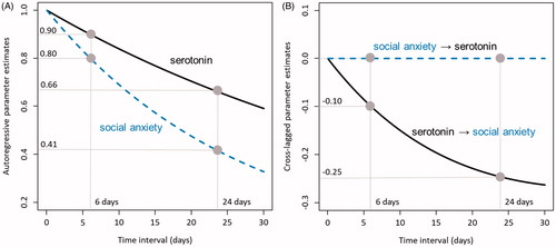
Going beyond just two selected intervals, the relationship between $\mathbf{A}$ and ${\mathbf{A}}^{*}\left(\Delta t_u\right)$ as a function of intervals $0<\Delta t\le 30$, is illustrated in Figure 3A for the autoregressive effects and in Figure 3B for the cross-lagged effects. Although the discrete time parameter estimates differ substantially as a function of the measurement intervals, the generating continuous time process is the same (i.e., the difference in discrete time estimates can be perfectly explained by the difference in time intervals).

Coming back to the original question of how should different time intervals be handled in the analysis and interpretation of results, we may conclude that continuous time modeling is a useful approach for doing so. In contrast to discrete time models, continuous time models prevent researchers arriving at different conclusions regarding the presence and size of an effect (e.g., from serotonin on social anxiety) simply because of the use of different data collection designs. Likewise, they prevent researchers from incorrectly interpreting similar discrete time effects, observed for different time intervals, as evidence for replicability without realizing that the true generating processes may have been very different.

However, discrete time analysis clearly has its place. In particular, in case of equally spaced measurement occasions with a high sampling frequency, which is completely under the researchers’ control (e.g., neurophysiological measures such as EEG data), discrete time models may be the better choice. They are mathematically simpler and computationally faster. Probably, the biggest disadvantage of continuous time dynamic models is that they are more difficult to implement in standard software packages. Only recently have a number of software packages for continuous time dynamic modeling been developed that overcome this limitation (e.g., ctsem, Driver, Oud, & Voelkle, 2017; OpenMx, Neale et al., 2016; BHOUM, Oravecz et al., 2016; dynr, Ou et al., 2017; see Singer, 1991, for an earlier program LSDE). By interfacing to OpenMx (Neale et al., 2016) and Stan (Carpenter et al., 2017; Stan Development Team, 2016), which are two powerful general purpose packages for frequentist and Bayesian data analysis, respectively, the R-package ctsem, for example, provides a user-friendly way to specify, estimate, and plot continuous time dynamic models. The software permits the analyses of time series data (T = large and N  =  1 or small) as well as panel data (N = large with T typically being small) and allows the basic model introduced in this paragraph to be extended in various ways. Most importantly, it permits (a) the estimation of multivariate reciprocal effects along with exogenous inputs (i.e., time-independent and time-dependent predictors) and (b) offers various options to account for heterogeneity across individuals, as discussed next.

Multivariate dynamic systems and interventions

The study of psychological mechanisms usually involves more than just one or two variables and effects are often not limited to unidirectional ones. Although the previously introduced mathematical models generalize readily to these cases, we want to draw attention to the role of time in interpreting such multivariate relationships. Without carefully considering the role of time in multivariate dynamic systems, one can easily arrive at contradictory conclusions. For example, as already suspected by the researcher from our running example, the effect of serotonin on social anxiety is unlikely to be a one-way effect. Rather, changes in social anxiety may also affect the levels of serotonin because a person experiencing increased levels of social anxiety may react by increasing the drug dosage. Furthermore, additional variables, such as social withdrawal behavior, may be important factors to consider when studying the relationship between social anxiety and serotonin. With three constructs, there exist six possible effects (lead-lag relationships) over time. Although in a stable bivariate model, the size of two discrete time effects may differ as a function of time, one will always remain stronger than the other (see Figure 3). This result is no longer true in the case of three or more variables. Figure 4 shows an example with the three variables social anxiety, serotonin, and social withdrawal behavior. As can be seen in Figure 4A, for time intervals between about one and about four weeks, the predicted effect of social anxiety on later serotonin is positive and is the strongest among all positive effects. In contrast, for some other time intervals (e.g., $\Delta t=6$), the effect is negative and comparatively weak. Thus, without considering how the dynamics of the system play out over the entire time range, it is easy to arrive at incorrect conclusions.

Figure 4. Example of a three-variate continuous time dynamic system of social anxiety, social withdrawal behavior, and serotonin. (A) Discrete time cross-lagged effects as a function of the time interval. (B) Hypothetical intervention on serotonin (e.g., via administration of an SSRI drug) at a time point t₀. (C) An alternative model with a single parameter modification as compared to the dynamic system displayed in Panel A (a_{withdrawal,social anxiety} = –0.2). (D) The same intervention as displayed in Panel B, based on the dynamic model shown in Panel C.

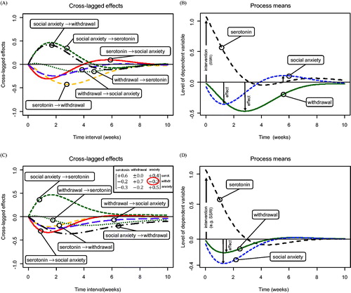
The importance of adequately accounting for time in the interpretation of effects is not limited to direct effects but generalizes readily to indirect effects. Recall that indirect effects are mediated by one or more processes (Cole & Maxwell, 2003; Maxwell, Cole, & Mitchell, 2011). In recent work, Deboeck and Preacher (2016) have demonstrated how the decomposition into direct, indirect, and total effects generalizes to continuous time dynamic models and how the unfolding of mediation effects over time can be visualized and tested. Understanding how effects unfold and decompose over time is particularly important when the goal is to develop effective interventions. Although many experimental studies settle for demonstrating the effect of an intervention at a single point in time (i.e., the measurement occasion), the researcher needs to keep in mind that the observed effect size is almost always a function of time. As illustrated in Figure 4B, in our example the administration of an SSRI drug increases the level of serotonin. Eventually, however, the effect will die out. More importantly, the intervention effect not only dissipates over time, but also leads to a decrease in social withdrawal behavior. Although only an indirect consequence of the intervention, the decrease in social withdrawal behavior in turn will result in an increase in social anxiety during the time period between about 4 and 8 weeks (dotted line). Without considering the complete time course of the effect, this complex dynamic interplay of the three variables would go undetected. For example, a randomized pre-post-test design on the effectiveness of an SSRI drug on social anxiety would suggest an increase in social anxiety if the post-test were administered 6 weeks after drug administration (see Figure 4B).

By including input effects (i.e., time-dependent predictors) in Equations 6(6) $$\frac{\mathrm{d}\mathbf{\eta }\left(t\right)}{\mathrm{d}t}=\mathbf{A}\cdot \mathbf{\eta }\left(t\right)+\mathbf{e},$$(6) and 7(7) $$\mathbf{\eta }\left(t_u\right)={\mathbf{A}}^{*}(\Delta t_u)\cdot \mathbf{\eta }\left(t_{u-1}\right)+\mathbf{\zeta }\left(t_u\right)\text{with}\mathbf{\zeta }\left(t_u\right)\sim \mathrm{N}\left(\mathbf{0},{\mathbf{Q}}^{*}\left(\Delta t_u\right)\right).$$(7) , we can study the time course of such interventions. The impulse effect illustrated in Figure 4B, which is the instantaneous effect of a single intervention (a single dosage of an SSRI drug) on the level of a dependent variable (serotonin), is one such possibility. Driver and Voelkle (in press-b) present a detailed consideration of how to study the time course of effects of interventions with continuous time dynamic models. They consider several types of input effects, such as persistent level changes, dissipative impulses, and oscillatory dissipation.

Considering the entire system and how effects change over time is not only important for studying the time course of interventions, it is also important when the goal is to change the system (e.g., to break a pathological system of relationships between social anxiety, withdrawal behavior, and SSRI drug usage). Imagine that our researcher had obtained a drift matrix of$\mathbf{A}=\left[\begin{array}{ccc}-0.3496& +0.0863& +0.6081\\ -0.1315& -0.2623& +0.6512\\ -0.4992& -0.2825& -0.4153\end{array}\right]$. Remember that the drift matrix contains the auto- and cross-effects of serotonin, social withdrawal behavior, and social anxiety in continuous time. This is the matrix underlying the pattern of effects shown in Figure 4A and Figure 4B, and corresponds to a discrete time autoregressive and cross-lagged matrix ${\mathbf{A}}^{*}\left(\Delta t=1\right)=\left[\begin{array}{ccc}+0.6& \pm 0.0& +0.4\\ -0.2& +0.7& +0.4\\ -0.3& -0.2& +0.5\end{array}\right]$, for a time interval of $\Delta t=1$ week. As is apparent in Figure 4 (panels A and B), a one-time administration of an SSRI drug to increase the level of serotonin is generally effective in the sense that it not only increases the level of serotonin, but also decreases social withdrawal behavior. While it initially also reduces social anxiety, the increase in social anxiety after about four weeks could be considered a negative side effect because it leads to a strong reduction in social withdrawal behavior. The key to avoiding this negative side effect would be to break the link between social anxiety and withdrawal behavior. An exposure therapy intervention could be one way to achieve this. By experimentally preventing withdrawal from a situation or encouraging social interactions when a patient experiences social anxiety, withdrawal behavior would no longer be a consequence of social anxiety. Withdrawal behavior would be fixed at a low level by the therapist. If our researcher succeeded in changing the effect of social anxiety on withdrawal behavior (i.e., $a^{*}(\Delta t=1)=+0.4$) from a positive effect into a small negative effect (e.g., $a^{*}(\Delta t=1)=-0.2$), the adverse effects of the intervention would disappear. This result is shown in Figure 4C and Figure 4D.

Formalizing and testing alternative dynamic models that differ in the strength of the links among its components and in how potential intervention effects play out over time may provide useful insights into clinical psychology and psychotherapy (see also Molenaar, 1987). Cognitive models of depression have long suggested that the relationship between negative cognitions and symptoms of depression constitutes a vulnerability factor to depression. Unlinking these factors is considered key to the success of cognitive therapy (Beevers & Miller, 2005).

To answer the question from our running example of how can we model and interpret reciprocal and mediation effects, and how do such effects manifest for any given time interval, important insights may be achieved if the researcher adopts a (multivariate) dynamic systems perspective. In a complex system, such as human cognition and behavior, a seemingly straightforward intervention on one variable can have complicated, potentially unintended, nonlinear effects on other outcome variables that show up over time. Simulating the consequences of an input by manipulating a variable (e.g., by administering a drug) or by changing the strength of the connection between two variables (e.g., by reducing the effect of social anxiety on withdrawal behavior) may lead to better understanding of such systems (e.g., the system illustrated in Figure 4) and the identification of promising interventions. This conclusion will be particularly true for complex models involving many variables. Although any parameter interpretation hinges on a correctly specified model, sensitivity analyses by means of simulations may also help to explore the potential impact of omitted variables in a multivariate dynamic system.

The role of time in the study of between-person differences and within-person changes

To sharpen the following discussion, it is useful to distinguish between five potential study designs as illustrated in Figure 5. Panel A shows a purely cross-sectional design, in which all individuals i  =  1, …, N are observed at a single time point t = t′. Panel B shows a time series design, in which a single individual i = i′ is observed at multiple time points t  =  1, …, T. Both are commonly used research designs, but not of focal interest for this article, because there is only a single source of variance in either design.

Figure 5. Illustration of five different study designs: A) time dimension is absent (t = t’; cross-sectional design); B) person dimension is absent (i = i’; time series design); C) person and time dimensions are perfectly crossed (all individuals are observed at all time points; panel design); D) person and time dimensions are not crossed (cross-sectional data at t = t’ and time series data for i = i’); E) partially crossed design (some individuals are observed at the same time points; panel design with missing data).

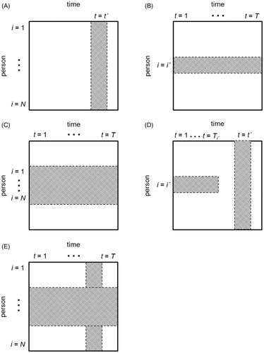
The distinct focus on either the BP and WP effects no longer holds for panels C and D. Panel C shows a design in which the time and person dimensions are perfectly crossed. Panel C is an example of a perfect panel design, in which the same group of individuals is observed at multiple time points. An important goal when using such data is to leverage information from multiple subjects in order to increase the precision of estimates and to study possible influences on interindividual differences. Fundamental to achieving this goal is to avoid confounding WP changes with BP differences. This observation raises the question: How should we deal with between-person differences in longitudinal panel data analysis? Panel D shows a design in which the time and person dimensions are both present but not crossed. This is the case if cross-sectional data are available for multiple individuals at a single point in time and time series data are available for a single subject across multiple time points. The researcher from our example confronts this case: She wants to translate findings from a BP cross-sectional study to a specific patient she has been monitoring over time. How can we compare and integrate results based on BP differences and those based on WP changes in our quest for causal mechanisms – or should we? In the following section, we will deal with the first question, before addressing the second.

The two conditions illustrated in Figure 5, panels C and D represent two idealized research designs. This distinction is useful in that it keeps separate the discussion of how we should analyze panel data (dimensions are fully crossed) from the discussion on the (in)compatibility of cross-sectional BP research and longitudinal WP research (dimensions are not crossed). In practice, the two dimensions may often be partially crossed as illustrated in Panel E. In this case, the two questions become at least partially confounded and need to be addressed depending on the research question and the location of the study design on the continuum between the two idealized conditions displayed in Panel C and Panel D.

Between-person differences in longitudinal panel data analysis

Inference on (causal) mechanisms may be based on BP data or WP data. Panel studies combine both types of data, providing advantages for improving causal inference, but also introducing new challenges for analyses. For a comprehensive introduction to causal inference in general, and from panel data in particular, see Morgan and Winship (2015), Imbens and Wooldridge (2009), and Hsiao (2014). In the following, we want to focus on one important challenge, namely, how to deal with unobserved unit heterogeneity. Unit heterogeneity refers to stable differences between units (typically people, i.e., BP differences) in the outcomes of interest. If the source of heterogeneity is known (e.g., sex differences), one speaks of observed heterogeneity that may be directly controlled for because its source is known. Often, however, the reasons for unit heterogeneity are many and varied, and so while some sources may be observed, many are not. If not adequately dealt with, the presence of unobserved heterogeneity may bias parameter estimates and result in incorrect conclusions. The information available from multiple subjects may also help to improve the estimation and avoid overfitting by regularizing the WP parameters away from extreme values (Bishop, 2006).

Unobserved heterogeneity as a source of confounding

Unobserved heterogeneity may bias parameter estimates in panel data analysis (cf. Halaby, 2004). One example in psychological research has recently been provided by Hamaker, Kuiper, and Grasman (2015), who criticized the discrete time cross-lagged panel model for its failure to adequately separate BP and WP levels in the presence of unobserved heterogeneity. These authors observed that stable differences across individuals are confounded with other (WP) parameter estimates, most importantly the cross-lagged effect parameters. As a solution, they proposed the inclusion of a random intercept – the so-called random intercept cross-lagged panel model (RI-CLPM). Controlling for unobserved heterogeneity by means of a random intercept can have dramatic effects on one’s results. Using empirical data, Hamaker et al. (2015) showed that high and significant autoregressive and cross-lagged effects (e.g., an autoregressive effect of .772 and cross-lagged effect of .115, both p<.001) may change dramatically to small and nonsignificant effects (.101 and .005, both p>.05) after accounting for unobserved heterogeneity by means of a random intercept.

By extending the latent state vector $\mathbf{\eta }\left(t\right)$ in Equation 6 (6) $$\frac{\mathrm{d}\mathbf{\eta }\left(t\right)}{\mathrm{d}t}=\mathbf{A}\cdot \mathbf{\eta }\left(t\right)+\mathbf{e},$$(6) (i.e., by adding additional latent variables) and constraining the corresponding auto-effect, the mean, and diffusion variance to zero, one can easily add random intercept terms to the continuous time equation. Due to the matrix exponential constraint described before (i.e., ${\mathrm{e}}^0=1$; see Equation 7(7) $$\mathbf{\eta }\left(t_u\right)={\mathbf{A}}^{*}(\Delta t_u)\cdot \mathbf{\eta }\left(t_{u-1}\right)+\mathbf{\zeta }\left(t_u\right)\text{with}\mathbf{\zeta }\left(t_u\right)\sim \mathrm{N}\left(\mathbf{0},{\mathbf{Q}}^{*}\left(\Delta t_u\right)\right).$$(7) ), the resulting autoregressive effects equal one, so that the freely estimated variances of the additional latent variables in $\mathbf{\eta }\left(t\right)$ capture all stable interindividual differences in the construct of interest. Technically, this situation corresponds to a random intercept vector in the stochastic differential equation, which is also referred to as a “trait” (Oud & Jansen, 2000; p. 200, Appendix A). This approach accounts for unit heterogeneity at the level of the latent variables. This approach differs slightly from accounting for unit heterogeneity in the measurement model as done, for example, in the RI-CLPM (Hamaker et al., 2015). In the RI-CLPM stable individual differences are treated as additive components at each observed measurement occasion, without implications for the underlying trajectory.³ Assuming that the model is identified, the two approaches may even be combined. However, identification may be rather complex and future research on this topic is necessary.

The inclusion of random intercepts is not the only way to deal with unobserved heterogeneity. As noted by Bollen and Brand (2010): “Researchers sometimes take false comfort in the use of the REM [random effects panel model] in that it does include a latent time-invariant variable (“individual heterogeneity”) without realizing that biased coefficients might result if the observed covariates are associated with the latent time invariant variable” (p. 2). The so-called fixed effects panel models are often proposed as a better alternative in such cases, because (unlike random effects panel models) they do not assume independence between unit-specific effects and potential time-varying regressors (Halaby, 2004). For example, by regressing on N-1 dummy variables, for N individuals, everyone would be assigned a person-specific intercept in a fixed effects model, without the need for any additional assumptions on distributions or covariances.

For dynamic panel models, fixed and random effects approaches can result in biased parameter estimates for finite T and N. Although various solutions for this problem have been proposed in the econometric literature (Arellano, 2003; Arellano & Bond, 1991), this remains an active field of research, with none of the proposed approaches being uniformly superior in terms of consistency, bias, and efficiency (Kiviet, 1995). Bollen and Brand (2010) recently proposed an SEM-based general panel model that incorporates both fixed and random effects. In their general panel model, traditional random and fixed effects can be considered as two special cases, which not only allows for a direct comparison of the two specifications, but also a mixture between the two (see also Allison, Williams, & Moral-Benito, 2017). This approach not only allows completely new modeling options, but (because of the SEM specification) also opens up the use of the fixed effects approach to dealing with unobserved heterogeneity in continuous time modeling. To the best of our knowledge, this has not yet been done; we encourage future research in this direction.

Unobserved heterogeneity as a source of information

Arguably, the most flexible approach is a fully hierarchical model, in which all parameters can vary across individuals, but information is still shared across individuals. This model includes all previously discussed models as special cases. In this model, a pure person-specific modeling approach (where a separate model is fit independently to each individual) and a modeling approach that ignores all BP differences (i.e., fits the same model to all individuals) represent the two extreme ends on a continuum.

The person-specific approach will yield consistent parameter estimates as T increases. However, the number of time points required for reasonable inference on even modestly complex models can be very large. A further issue is that finite sample biases, such as that seen in the autoregressive parameter (Marriott & Pope, 1954), ensure that in typical contexts, the person-specific approach suffers from both high uncertainty of the estimates and substantial biases. Although the other extreme of ignoring BP differences is also untenable (for reasons already discussed), the random effects approach may be seen as a middle-ground between the two extremes. Rather than either “no variation in parameters across subjects” or “entirely independently estimated parameters across subjects,” the random effects approach results in subject-level parameters that are based on a mixture of WP and BP information. In a frequentist random effects formulation, wherein the subject-level parameters are not directly estimated but rather only the population distribution of the parameters is estimated, this result is not always so apparent. However, if one considers a typical Bayesian approach, in which the subject-level parameters are estimated along with the population distribution, the population distribution provides the prior for the subject-level parameters. This prior then results in a regularization of the subject-level parameters away from extremes, toward the population mean – with the extent of this regularization being dependent on how much information is available for the specific subject and the population as a whole (Bishop, 2006). If the variance of the random effects was fixed in advance to zero, the model is equivalent to the “ignore BP differences” approach; conversely, the model approaches that of the “person-specific, independent parameters” approach (Driver & Voelkle, in press-a) if the variance was fixed to a very high value. By estimating the variance, we can, to a reasonable extent, optimize parameter estimation in that both BP and WP sources of information are optimally leveraged.

For identification and estimation purposes, certain constraints on the population distribution of the parameters may be necessary. The assumption of a normally distributed intercept with zero mean and a certain variance in the RI-CLPM is an example of such a constraint. In addition, certain caveats apply, such as requiring a sufficiently complex model to accommodate all individuals (see Liu, 2017). For complex models with multiple individually varying parameters, a hierarchical Bayesian formulation offers the necessary flexibility for model specification and estimation. These models require that hyperpriors on the population distribution of model parameters need to be specified; the hyperpriors determine the degree to which parameters can differ across individuals. For work on hierarchical Bayesian continuous time dynamic models in psychological research, see Oravezc et al. (2009, 2011, 2016), and for a recent extension of the ctsem software to fully hierarchical Bayesian models by means of stan, see Driver and Voelkle (in press-a).

In this section, we have outlined different approaches to address the researcher’s question how should she deal with between-person differences in longitudinal panel data analysis? Most importantly, unit heterogeneity should be recognized and represented in the model to avoid the risk of confounded and substantively meaningless parameter estimates. Random and fixed effects approaches are both suitable to account for such unobserved heterogeneity, with each having advantages and disadvantages depending on the situation. By specifying hyperpriors, hierarchical Bayesian models allow users to determine the degree to which they may allow for individual differences in parameter estimates, ranging from no differences across all individuals to independent parameter estimates for each individual as the two end points on this continuum.

Between-person differences and within-person changes in the quest for causal mechanisms

We now turn to the situation when the time and person dimension are not crossed (see Figure 5D). In our running example, the researcher was worried by the perceived discrepancy between the medium-to-strong negative correlation of serotonin and social anxiety reported in previous cross-sectional studies and her own clinical experience with her individual patients. Indeed, as will be shown in the next section, from a statistical perspective, the assumptions necessary for a straightforward generalization from a BP finding to an individual are unlikely to be met. However, does this imply that nothing can be learned from BP differences about WP effects? Should our researcher ignore findings from cross-sectional (BP) studies when aiming to understand the relationship between serotonin and social anxiety in a given patient? After first considering the statistical perspective, we will next argue from a causal perspective that such a conclusion seems premature. We will then outline a way to reconcile these two perspectives.

The statistical perspective

From a statistical perspective, it is not surprising that an effect observed at the BP level may be very different from an effect observed at the WP level. What is surprising and somewhat bewildering is the ease with which researchers sometimes switch between the two levels in the interpretation and communication of findings related to complex psychological constructs such as personality or intelligence (cf. Borsboom, Mellenbergh, & van Heerden, 2003; Borsboom & Dolan, 2006; Franic, Borsboom, Dolan, & Boomsma, 2014; Valsiner, 1986; see Kluckhohn & Murray, 1953 for a classic treatment). With a “a manifesto on psychology as idiographic science,” Molenaar (2004, p. 201) demonstrated these problems to the scientific community by providing a proof that, from a mathematical statistical perspective, a generalization from the BP level to the WP level is usually not warranted. Based on classic theorems of ergodic theory, he argued that “only under very strict conditions – which are hardly obtained in real psychological processes – can a generalization be made from a structure of interindividual variation to the analogous structure of intraindividual variation” (Molenaar, 2004, p. 201). For such a generalization to be valid, the same model needs to apply to all individuals (homogeneity) and all individual processes need to be stationary, containing no systematic trends or cycles. Homogeneity and stationarity are the two conditions for so-called “ergodicity” (Molenaar & Campbell, 2009, p. 113; Molenaar, 2004, pp. 206–207; making some simplifying assumptions, such as multivariate normality). Appendix A provides a formal statement of the conditions under which ergodicity will be met.

Given that there are systematic interindividual differences (heterogeneity) as well as systematic changes (non-stationarity) in almost all psychological constructs, the observation of the researcher from our running example should not come as a surprise nor should the lack of generalizability from BP findings to WP findings and vice versa. It is this disconnect that underlies the call for a “new person-specific paradigm” in psychology (Molenaar & Campbell, 2009, p. 112). From this statistical perspective, the researcher from our example would be well-advised not to rely on existing cross-sectional studies when her goal is to understand and treat an individual patient. This insight implies that, despite the effectiveness of SSRIs demonstrated in previous RCTs, our researcher cannot know whether an SSRI drug will be effective for a given patient without homogeneity assumptions.

The causal perspective

Instead of taking a statistical perspective and asking under which conditions BP and WP estimates will be equivalent, we can also ask what caused the data? It is this slight change from a statistical perspective to a causal perspective that may result in a somewhat different recommendation to our researcher.

For the purpose of the present article, we adopt the general definition of a causal effect as the interventional distribution $P(Y=y|do\left(x´\right),\mathcal{M})$ for a given Model $\mathcal{M}$ (cf. Hauser & Bühlmann, 2015; Pearl, 1995, 2009; Shpitser & Pearl, 2006). The do() operator simulates an external intervention by setting the value of a variable X to a fixed value x´. The action of setting X to x´, as compared to passively observing X = x´, is denoted by do(x´). Of importance, setting X to a specific value x´ implies “wiping out” the equation from model $\mathcal{M}$ that usually determines the value of X and replacing it by the equality X = x´. The corresponding probability for Y = y, given the intervention do(x´) is $P(Y=y|do\left(x´\right))$. Note that the intervention do(x´) may be purely hypothetical. To define and identify a causal effect, it is not necessary that it is actually possible to manipulate the physical world by setting X to x´. Furthermore, in its general form, the definition of a causal effect as the interventional distribution $P(Y=y|do\left(x´\right),\mathcal{M})$ is not restricted by any parametric assumptions. In practice, however, it is often useful to assume a parametric model and to focus on specific aspects of a causal effect, such as the expected change in a dependent variable Y for a marginal change in the interventional level x´ for model $\mathcal{M}$ and parameter vector $\mathbf{\theta }$ as shown in Equation 8(7) $$\mathbf{\eta }\left(t_u\right)={\mathbf{A}}^{*}(\Delta t_u)\cdot \mathbf{\eta }\left(t_{u-1}\right)+\mathbf{\zeta }\left(t_u\right)\text{with}\mathbf{\zeta }\left(t_u\right)\sim \mathrm{N}\left(\mathbf{0},{\mathbf{Q}}^{*}\left(\Delta t_u\right)\right).$$(7) : (8) $$\frac{\mathrm{d}}{\mathrm{d}{x}^{\prime }}E\left(Y=y|do\left(x^{\prime }\right),\mathcal{M}\left(\mathbf{\theta }\right)\right).$$(8)

For illustration, but without loss of generality, we will focus on this specific notion of a causal effect as the sensitivity of the mean of Y to changes in the interventional level x´ (mean vectors Y and X in case of multiple dependent and independent variables).

Building upon graph theory, Pearl and others (Pearl, 2009; Shpitser & Pearl, 2006) have developed a set of mathematical rules to decide whether or not a causal effect is identified and can be inferred from observational data. These rules are based on the so-called directed acyclical graphs (DAGs), graphical representations of a model $\mathcal{M}$. In the following, we propose that DAGs can be used for causal inference, irrespective of whether the data are collected at the BP level or the WP level, and that we can use the same set of mathematical rules for causal effect identification. This idea is illustrated in Figure 6, and a proof-of-concept is provided in Appendix B.

Figure 6. Two illustrative examples of a BP model (A) and a WP model (B). Each model is graphically illustrated by a directed acyclical graph (above the dashed lines). The causal effects of interest are X→Y in the BP model and $X_{t=2}$ → $X_{t=3}$ in the WP model. The corresponding interventional distributions are shown below the dashed lines. Identification of the marginal causal effect of X on Y may be achieved by controlling for Z in Model A. Identification of the marginal causal effect of $X_{t=2}$ on $Y_{t=3}$ may be achieved by controlling for $Y_{t=2}$, $X_{t=1}$ or $\left\{Y_{t=2}, X_{t=1}\right\}$ in Model B.

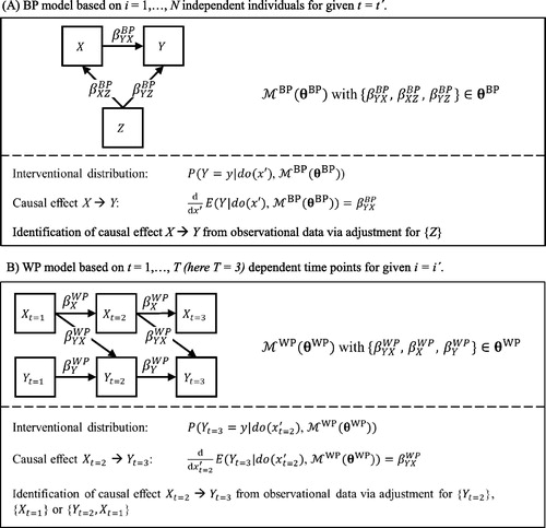
Figure 6 shows two different DAGs to infer a causal effect of X on Y. Panel A in Figure 6 shows a BP model based on i  =  1,…, N independent individuals for a given time point t  =  t´, whereas Panel B shows a WP model based on t  =  1,…, T (here, T  =  3) dependent time points for a given individual i  =  i´. In line with our running example, variable X may represent serotonin, Y may represent social anxiety, and Z may represent sex. The causal quantity, as defined in Equation 8(7) $$\mathbf{\eta }\left(t_u\right)={\mathbf{A}}^{*}(\Delta t_u)\cdot \mathbf{\eta }\left(t_{u-1}\right)+\mathbf{\zeta }\left(t_u\right)\text{with}\mathbf{\zeta }\left(t_u\right)\sim \mathrm{N}\left(\mathbf{0},{\mathbf{Q}}^{*}\left(\Delta t_u\right)\right).$$(7) , is equal to ${\beta }_{YX}^{BP}$ for the effect of serotonin on social anxiety. From the corresponding DAG, it is apparent that we can identify the causal effect from purely observational data if we control for variable Z (i.e., by applying the so-called back-door criterion; Pearl, 2009). Likewise, in the WP model illustrated in Figure 6B, we can identify the causal effect quantity ${\beta }_{YX}^{WP}$ of serotonin at t  =  2 on social anxiety at t  =  3 by controlling for (a) variable $X_{t=1}$, or (b) $Y_{t=2}$, or (c) variables $X_{t=1}$ and $Y_{t=2}$ (for proof, see Appendix B).

Although statistically the BP relationship between Y and X is unlikely to be identical to the WP relationship between Y and X, this example illustrates that it is possible to infer causal information about the effect of X on Y from either the BP model ${\mathcal{M}}^{\text{BP}}$ or the WP model ${\mathcal{M}}^{\text{WP}}$. Of importance, the conditions under which such causal inference is possible differ across the BP and WP model: First, the two DAGs (i.e., model structure ${\mathcal{M}}^{\text{BP}}$ vs. ${\mathcal{M}}^{\text{WP}}$) differ and, second, we need to adjust for different sets of variables for causal identification (i.e., controlling for {Z} in the BP model vs. controlling for {X_{t = 1}}, {Y_{t = 2}} or {X_{t = 1}, Y_{t = 2}} in the WP model). In addition, the number of parameters in the BP and WP model may differ (i.e., the length of ${\mathbf{\theta }}_{i=i´}^{\text{WP}}$ vs. ${\mathbf{\theta }}_{t=t´}^{\text{BP}}$ may differ).

Toward a unified paradigm

To reconcile the statistical fact that a generalization from the BP level to the WP level is usually not warranted with the insight that both levels may contribute to a better understanding of the same psychological mechanisms, Voelkle, Brose, Schmiedek, and Lindenberger (2014) highlighted the importance of distinguishing between parameters that are unique to a BP or WP model and parameters that are common to both. In the following, we denote the former by subscript u, and the latter by subscript c. Instead of simply comparing ${\mathbf{\theta }}_{i=i´}^{\text{WP}}$ to ${\mathbf{\theta }}_{t=t´}^{\text{BP}}$, this allows us to test for conditional equivalence by controlling for factors that are unique to either the BP or WP level (i.e., to compare $\left({\mathbf{\theta }}_{\mathrm{c}, i=i´}^{\text{WP}}|{\mathbf{\theta }}_{\mathrm{u}, i=i´}^{\text{WP}}\right)$ to $\left({\mathbf{\theta }}_{\mathrm{c},t=t´}^{\text{BP}}|{\mathbf{\theta }}_{\mathrm{u}, t=t´}^{\text{BP}}\right)$).

For example, the effects ${\mathbf{\theta }}_{\mathrm{u}, t=t´}^{\text{BP}}=\{{\beta }_{XZ}^{BP}, {\beta }_{YZ}^{BP}\}$ of variable Z in Figure 6A represent sex differences in serotonin and social anxiety. These effects are unique to the BP model and may explain part of the unconditional relationship between serotonin and social anxiety (e.g., Nishizawa et al., 1997). Given that sex differences only exist between different people, it is neither necessary nor possible to explicitly control for Z at the WP level. However, unlike at the BP level, there exist serial dependencies between measures across time, captured by the parameters ${\mathbf{\theta }}_{\mathrm{u}, i=i´}^{\text{WP}}=\{{\beta }_X^{WP}, {\beta }_Y^{WP}\}$, which are unique to the WP level. Before drawing any comparisons regarding the effect of X on Y, which is captured by the common parameter ${\mathbf{\theta }}_{\mathrm{c},t=t´}^{\text{BP}}=\left\{{\beta }_{XZ}^{BP}\right\}\stackrel{?}{=}{\mathbf{\theta }}_{\mathrm{c},i=i´}^{\text{WP}}=\left\{{\beta }_{XZ}^{WP}\right\}$, it is necessary to control for factors that are unique to either of these two levels. The comparison can be carried out, for example, by means of likelihood ratio tests as described in detail by Voelkle et al. (2012, 2014).

The problem with this approach is that there exist many different factors that could be controlled for at either level, and previous research has been mute on how to choose them. We propose to solve this problem by means of DAGs and existing rules for causal identification (such as the backdoor or frontdoor criterion, Pearl, 2009), so that the common parameters capture the causal mechanisms of interest. Although the modeling should be done in a single step (see Voelkle et al., 2014), it is heuristically useful to think of this as a three-step process: First, we make use of the well-established causal inference machinery based on DAGs to obtain an estimate of the causal effect X on Y from a BP model ${\mathcal{M}}^{\text{BP}}$. Second, we use the same machinery to obtain an estimate of the causal effect of X on Y from the WP model ${\mathcal{M}}^{\text{WP}}$. Third, if steps 1 and 2 are successful, then the two causal effects may be tested against each other. Only in the case of equivalence is it viable to generalize from the BP level to a causal mechanism at the WP level or vice versa. Only in that case would it be justified to administer a certain intervention to an individual patient based on a causal structure that was originally inferred from a BP study and then found to adequately represent this specific patient’s WP data. For example, our researcher could directly translate the average causal effect of serotonin on social anxiety from an RCT to a given patient.

Obviously, in the social and behavioral sciences such perfect equivalence seems unlikely, and, depending on the research question, researchers may resort to different criteria to determine equivalence (cf. Anderson & Maxwell, 2016). Likewise, the comparison of a single BP structure for t = t′ and fixed N, with a single WP structure for i = i′ and fixed T, constitutes an extreme condition (see Figure 5D). This condition was deliberately chosen to sharpen the discussion and illustrate our arguments but may not be prototypical for applied research. With sufficiently many time points and individuals, there is also no need for such comparisons. In practice, such comparisons become increasingly relevant when (a) individual differences exist in the degree of equivalence and (b) the amount of available data differs at the BP and WP level. Regarding (a), Brose, Voelkle, Lövdén, Lindenberger, and Schmiedek (2015) made use of the COGITO data to assess the degree of BP and WP equivalence in the structure of affect by means of likelihood ratio tests as outlined above. They rank-ordered individuals based on the degree of (non-) equivalence and demonstrated that the degree of non-equivalence is related to well-being and stress. Regarding (b), especially in clinical settings, a treatment decision on an individual patient is often necessary upon the first encounter with this patient. For example, our practicing clinician may need to decide at intake whether or not to prescribe a new patient an SSRI drug. No longitudinal WP information is available for this patient so that this decision can only be made based on BP information (i.e., previous RCTs). However, after the patient returns for several follow-up visits, WP data on the effectiveness of the treatment become available. With increasing WP information (increasing T), the question arises whether the observed WP effect is equivalent or deviates from the initially expected BP effect. How to optimally integrate BP and WP information in the improvement of medical decision-making remains an important task for future research. A naïve approach, for example, could be to base the individual treatment decision on the average causal effect estimate from the BP information until the accumulated evidence at the WP level suggests a (significant) deviation from the expected BP causal effect estimate.

Returning to the question of the researcher from our running example (how can we compare and integrate results based on BP differences and results on WP changes in our quest for causal mechanisms – or should we?) we conclude the following: As pointed out by Molenaar and others (2004; Molenaar & Campbell, 2009; Valsiner, 1986), from a statistical perspective a generalization of results based on BP difference to WP changes is only justified under very strict assumptions, which are unlikely to be valid in practice. Thus, great caution is indicated when the goal is to infer WP relationships from BP data or vice versa. Both levels, however, can be informative for causal inference. Based on rules for causal inference by means of DAGs, our researcher can decide which variables to control for (or not control for) at either level. Conditional on these variables she can assess the degree of equivalence of those subsets of the BP and WP model parameters that capture the causal effects of interest. When the relevant parameters are reasonably similar, a generalization from the BP to the WP level will be warranted; if they are not, such generalization is impossible.

Although we believe this approach to dealing with the division of BP and WP research offers a more practical and more nuanced perspective on how we can – or should – integrate these different sources of information, it is not without problems: First and foremost, it hinges on a correctly specified causal model (DAG). This limitation is shared with all causal inference approaches based on DAGs. In practice, sensitivity analyses and robustness checks are necessary to safeguard against false conclusions due to incorrectly specified causal models. Second, a longitudinal DAG, by definition, represents a discrete time model. The causal parameters refer to a specific discrete time interval. As illustrated in Figure 4, Panel B, the causal effect of an input will manifest itself differently at different time points. Thus, the comparison of a WP to a BP causal effect depends on an adequately chosen time interval. Continuous time modeling may help to overcome this limitation because it permits the derivation of the expected discrete time effects for any arbitrary time interval. In an exploratory way, one could thus derive the time interval at which a WP effect is most similar to a BP effect (e.g., by simple plotting of the expected effects as shown Figure 4, Panel B). Using a confirmatory approach, one could specify the WP DAG at the (BP) time interval of interest, prior to any comparisons of the WP to the BP causal structure. In both cases, however, future research seems necessary to test and refine the approach to causal inference by paying closer attention to the role of time (cf. Zhang, Joffe, & Small, 2011).

Discussion

Without considering time, the study of psychological mechanisms is impossible. At the very least, the cause must precede the effect in time, or else a cause-effect relationship can be ruled out for most practical purposes (Shadish, Cook, & Campbell, 2002). Even the classical randomized controlled trial as the “gold standard” for causal inference assumes that the treatment takes place prior to the measurement of the dependent variable (Holland, 1986; Shadish et al., 2002) and that the effect size may depend on the time interval between the treatment and the outcome measurement (e.g., Figure 4, Panel B). Adequately considering the role of time in the study of psychological mechanisms becomes even more important in observational longitudinal studies. Neither under laboratory conditions nor in real life can the phenomena of interest be continuously observed. In addition, the outcome variables often exhibit complex relationships across time with large WP variation and BP differences. How can we best make use of the available information in analysis and interpretation? Along five prototypical questions, we identified several common problems in the longitudinal study of psychological mechanisms and discussed how they can be resolved by paying closer attention to the role of time.

To address the question “What statistical model should one use to best understand possible mechanisms?” we distinguished between two broad classes of longitudinal models: static models and dynamic models. While both classes offer powerful approaches for the analysis of change, we encouraged researchers to consider the use of dynamic modeling approaches when they seek to study psychological mechanisms. With this recommendation, we echo McArdle’s (2009) earlier call to start the analysis of longitudinal data not by asking “What is your data collection design?” but rather by asking “What is your model for change?” (p. 601).

To address the question “How should different time intervals be handled in the analysis and interpretation of results?” we distinguished between discrete and continuous time models. We recommend that the time variable should usually not be discretized, but rather treated as a continuous variable. Although this is straightforward in static models of change, the situation is more complicated in dynamic models of change. Building upon a short review of latent change score models, we introduced the basic idea of continuous time dynamic modeling that resolves many previous problems in treating time as a continuous variable in dynamic models.

To address the question “How can we model and interpret reciprocal and mediation effects and how do such effects manifest for any given time interval?,” we recommended researchers adopt a dynamic systems perspective. We demonstrated how in a multivariate system, apparently simple interventions (e.g., an increase in serotonin in Figure 4B or D) may result in complicated, potentially unintended, nonlinear effects on other variables that only show up over time. We distinguished between manipulating a variable in a system (e.g., increasing the level of serotonin) and changing the effect of one variable on another (e.g., decreasing, or eliminating, the effect of social anxiety on withdrawal behavior; see Figure 4C) and sketched how both may advance our understanding of psychological mechanisms (see also Butner, Gagnon, Geuss, Lessard, & Story, 2015).

To address the question “How should we deal with between-person differences in longitudinal panel data analysis?,” we highlighted the dual role of BP differences as a potential source of confounding as well as a source of information. To avoid confounded and substantively meaningless parameter estimates, we advised researcher to carefully control for unobserved heterogeneity in longitudinal panel data. However, we also recommended leveraging information from multiple subjects to improve the precision of (WP) estimates. It is important to note that these two recommendations generally do not contradict each other. Unless we have a very large number of measurement occasions per individual, a purely person-specific approach (i.e., treating an individual as completely independent of all other individuals) is likely to overfit the data and yield biased parameter estimates. Likewise, ignoring unobserved heterogeneity (i.e., treating all individuals alike) will result in confounded and substantively meaningless parameter estimates, unless there are indeed no systematic differences among individuals. Leveraging both WP and BP sources of information, according to the information provided by each source (as is done by hierarchical models), effectively eliminates the apparent contradiction.

To address the question “How can we compare and integrate results based on BP differences and those based on WP changes in our quest for causal mechanisms – or should we?” researchers need to think hard about the correct causal model at either level (e.g., by formulating the corresponding DAGs). In practice, these models can be expected to differ from each other. Making use of rules for causal inference, researchers should identify the variables that need to be controlled (or not controlled) at either level before assessing the degree of equivalence of BP and WP model parameters that capture the causal effects of interest, conditional on these factors. Given correctly specified DAGs, adequately controlling for these factors permits the identification of common underlying causal mechanisms and may thus provide a way to unify the BP and WP research paradigms in psychology (cf. Beltz, Wright, Sprague, & Molenaar, 2016; Borsboom, Kievit, Cervone, & Hood, 2009; Cronbach, 1957, 1975; Voelkle et al., 2014). This effort at unification requires the translation of theories into causal structures that govern the evolution of dynamic systems.

Current limitations and future directions

More than forty years ago, Baltes, Reese, and Nesselroade remarked that “[w]hatever kind of theoretical model a given researcher chooses to adopt, it seems fair to argue that a time-ordered analysis of networks of antecedent variables will be useful in understanding and controlling behavior” (1988, p. 106). Since then, methodologists and statisticians have made great progress in designing tools that facilitate the analysis of multivariate longitudinal data. Nevertheless, two broad categories of limitations continue to hamper the “time-ordered analysis of networks of antecedent variables” that Baltes and colleagues were advocating.

First, statistical and computational difficulties continue to exist. In particular, multivariate continuous time dynamic models of multiple latent processes can be difficult to fit. While mathematically and in terms of available software packages, there is no theoretical upper limit for the number of manifest and latent variables, at least for panel data, few researchers have attempted to model more than just a few latent processes. Reasonably chosen (hyper)priors in Bayesian model estimation may mitigate small sample problems and problems of complexity, but computational problems remain and need to be addressed in future research. Finding a solution to statistical and computational problems becomes even more important when considering not only heterogeneity across individuals but also heterogeneity across time. Although considerable attention has been devoted to the former, heterogeneity across time has been largely ignored in the present article. With increasing durations of time series data in psychological research, this problem becomes increasingly pressing (for recent work on changing dynamics in discrete time series, see Bringmann et al., 2017; Molenaar, Sinclair, Rovine, Ram, & Corneal, 2009; for work on continuous time models, see Chen, Chow, & Hunter, in press; Oud & Jansen, 2000).

The second impediment to progress is conceptual in nature. While better software and increased computing power will eventually overcome or attenuate most statistical and computational problems, our perspective also points to an urgent need for theories that specify the temporal properties of the system under investigation with greater precision, based on evidence about its components and their configuration. Many researchers are quick to acknowledge that human behavior is best understood as a highly flexible, complex, dynamical system. However, this perspective is not reflected in the vast majority of psychological research and theorizing, where “dynamics” is often little more than a buzzword (Voelkle, 2015). Theorizing about human behavior is often poorly specified in the time domain. A useful contrast is to examine examples of research on other living systems that has made greater progress in appreciating the role of time. A prominent example is research on the heart, where knowledge about the time constants of its components and their configuration into a system has resulted in a thorough, non-reductionist understanding of causality at the system level (e.g., Noble, 2007, 2012). Given the increasing availability of methods to study the dynamics of human behavior (e.g., Boker & Wenger, 2007; Chow, Ferrer, & Hsieh, 2009), the time has come to interrogate psychological theories on what they have to say about the time constants and configuration of major components of the hypothesized system.

Bridging the gap between the development of formal quantitative methods and their application is important but not always easy. Better education and, in particular, more interdisciplinary collaboration are necessary to accomplish this task. As pointed out before, both statistical models for studying human dynamics and conceptual research on causal inference from the observational data have improved significantly in recent years (cf. Imbens & Rubin, 2015; Imbens & Wooldridge, 2009; Morgan & Winship, 2015; Pearl, 2009). A better integration of these lines of inquiry seems key in the search for psychological mechanisms. Our hope is that the approach sketched in the present paper is a first small step in this direction.

Article information

Conflict of interest disclosures: Each author signed a form for disclosure of potential conflicts of interest. No authors reported any financial or other conflicts of interest in relation to the work described.

Ethical principles: The authors affirm having followed professional ethical guidelines in preparing this work. These guidelines include obtaining informed consent from human participants, maintaining ethical treatment and respect for the rights of human or animal participants, and ensuring the privacy of participants and their data, such as ensuring that individual participants cannot be identified in reported results or from publicly available original or archival data.

Funding: This work was not supported.

Role of the funders/sponsors: None of the funders or sponsors of this research had any role in the design and conduct of the study; collection, management, analysis, and interpretation of data; preparation, review, or approval of the manuscript; or decision to submit the manuscript for publication.

Acknowledgments

The present article is based on a presentation given by the first author at the COGITO conference, October 4-6, 2016, Max Planck Institute for Human Development, Berlin, Germany. We are indebted to the associate editor and an anonymous reviewer for their insightful comments and for providing directions that have resulted in the present paper. We acknowledge support by the Open Access Publication Fund of Humboldt-Universität zu Berlin. We also thank Han Oud and the members of the Methods Group Berlin for the inspiring and always interesting discussions and insights on the role of time in our quest for better understanding psychological mechanisms. The ideas and opinions expressed herein are those of the authors alone, and endorsement by the authors' institutions is not intended and should not be inferred.

Notes

1 For example, dynamic and static models may be combined by augmenting a “dynamic” model by a static component or vice versa (e.g., a “static” linear growth curve model could be augmented by a dynamic AR(1) process or a “dynamic” panel model could be augmented by a linear mean trajectory). Likewise, we can restrict the parameters of a dynamic model in such a way that the dynamics are eliminated, thus reducing it to a static model.

2 More precisely, $\mathbf{e}=\mathbf{G}\frac{\mathrm{d}\mathbf{W}\left(t\right)}{\mathrm{d}t}$, with $\mathbf{W}\left(t\right)\in R^v$ denoting the Wiener process, a random walk in continuous time. $\mathbf{G}\in R^{v\times v}$ is the Cholesky matrix with diffusion matrix $\mathbf{Q}=\mathbf{G}{\mathbf{G}}^{\mathrm{T}}$. For a derivation of the exact relationship between the discrete and continuous time error covariance matrix, see Voelkle et al. (2012, Appendix C) and the additional references provided therein. We also note that it is common (and in strict mathematical terms more precise) to multiply both sides of Equation 6 by dt, resulting in $\mathrm{d}\mathbf{\eta }\left(t\right)=\mathbf{A}\mathbf{\eta }\left(t\right)\mathrm{d}t+\mathbf{G}\mathrm{d}\mathbf{W}\left(t\right).$ We treat these expressions as equivalent.

3 The package ctsem allows users to switch between these two specifications.

Appendix A

Let ${\mathbf{\theta }}_{i=i´}^{\text{WP}}$ be the parameter vector of a WP model ${\mathcal{M}}^{\text{WP}}\left({\mathbf{\theta }}_{i=i´}^{\text{WP}}\right)$for a given individual i  =  i´. Furthermore, let ${\mathbf{\theta }}_{t=t´}^{\text{BP}}$ be the parameter vector of a BP model ${\mathcal{M}}^{\text{BP}}\left({\mathbf{\theta }}_{t=t´}^{\text{BP}}\right)$for a given time point t  =  t´. Equivalence of BP and WP parameters for individual $i=i´$ and time point $t=t´$ is given if ${\mathbf{\theta }}_{i=i´}^{\text{WP}}={\mathbf{\theta }}_{t=t´}^{\text{BP}}$. For example, assuming multivariate normality and a saturated model with free mean vector $\mu$ and covariance matrix $\Sigma$, that is, ${\mathcal{M}}^{\text{BP}}\left({\mathbf{\theta }}_{t=t´}^{\text{BP}}=\{{\mathbf{\mu }}_{t=t´},{\Sigma }_{t=t´}\}\right)$ and ${\mathcal{M}}^{\text{WP}}\left({\mathbf{\theta }}_{i=i´}^{\text{WP}}=\{{\mathbf{\mu }}_{i=i´},{\Sigma }_{i=i´}\}\right)$, the BP and WP structure for individual $i=i´$ and time point $t=t´$ would be equivalent if $\left\{{\mathbf{\mu }}_{t=t´},{\Sigma }_{t=t´}\right\}=\{{\mathbf{\mu }}_{i=i´},{\Sigma }_{i=i´}\}$. Ergodicity is met if ${\mathbf{\theta }}_i^{\text{WP}}={\mathbf{\theta }}_t^{\text{BP}}$ for all possible combinations of i  =  1, …, N and t  =  1, …, T.

Appendix B

The directed acyclical graph (DAG) displayed in Panel A of Figure 6 corresponds to the following set of structural equations: $$\left(\begin{array}{c}Z\\ X\\ Y\end{array}\right)=\left(\begin{array}{ccc}0& 0& 0\\ {\beta }_{XZ}^{BP}& 0& 0\\ {\beta }_{YZ}^{BP}& {\beta }_{YX}^{BP}& 0\end{array}\right)\left(\begin{array}{c}Z\\ X\\ Y\end{array}\right)+\left(\begin{array}{c}{\epsilon }^Z\\ {\epsilon }^X\\ {\epsilon }^Y\end{array}\right)$$

Under the intervention $do\left(x^{\prime }\right)$ the structural equations are given by the following: $$\left(\begin{array}{c}Z\\ X\\ Y\end{array}\right)|do\left(x^{\prime }\right)=\left(\begin{array}{ccc}0& 0& 0\\ 0& 0& 0\\ {\beta }_{YZ}^{BP}& {\beta }_{YX}^{BP}& 0\end{array}\right)\left(\begin{array}{c}Z\\ X\\ Y\end{array}\right)+\left(\begin{array}{c}{\epsilon }^Z\\ 0\\ {\epsilon }^Y\end{array}\right)+\left(\begin{array}{c}0\\ x^{\prime }\\ 0\end{array}\right)$$

Since the system is recursive, it has a unique solution given by the following: $$\left(\begin{array}{c}Z\\ X\\ Y\end{array}\right)|do\left(x^{\prime }\right)=\left(\begin{array}{c}{\epsilon }^Z\\ x^{\prime }\\ {\beta }_{YX}^{BP}{x}^{\prime }+{\beta }_{YZ}^{BP}{\epsilon }^Z+{\epsilon }^Y\end{array}\right)$$

Following the definition of a causal effect as given in Equation 8(7) $$\mathbf{\eta }\left(t_u\right)={\mathbf{A}}^{*}(\Delta t_u)\cdot \mathbf{\eta }\left(t_{u-1}\right)+\mathbf{\zeta }\left(t_u\right)\text{with}\mathbf{\zeta }\left(t_u\right)\sim \mathrm{N}\left(\mathbf{0},{\mathbf{Q}}^{*}\left(\Delta t_u\right)\right).$$(7) , the causal effect of $X$ on $Y$is given by the following: $$\frac{\mathrm{d}}{\mathrm{d}x\prime }E\left(Y|do\left(x^{\prime }\right),{\mathcal{M}}^{\text{BP}}\left({\mathbf{\theta }}^{\text{BP}}\right)\right)=\frac{\mathrm{d}}{\mathrm{d}x\prime }E\left({\beta }_{YX}^{BP}{x}^{\prime }+{\beta }_{YZ}^{BP}{\epsilon }^Z+{\epsilon }^Y\right)={\beta }_{YX}^{BP}$$

The DAG displayed in Panel B of Figure 6 corresponds to a first-order bivariate vector autoregressive process. The corresponding equations together with the initial values ($t=1$) are given by the following: $$\begin{array}{c}\left(\begin{array}{c}{X}_t\\ Y_t\end{array}\right)=\left(\begin{array}{cc}{\beta }_X^{WP}& 0\\ {\beta }_{YX}^{WP}& {\beta }_Y^{WP}\end{array}\right)\left(\begin{array}{c}{X}_{t-1}\\ Y_{t-1}\end{array}\right)+\left(\begin{array}{c}{\epsilon }_t^X\\ {\epsilon }_t^Y\end{array}\right) t=2,\dots ,T\\ \left(\begin{array}{c}{X}_{t=1}\\ Y_{t=1}\end{array}\right)=\left(\begin{array}{c}{\epsilon }_{t=1}^X\\ {\epsilon }_{t=1}^Y\end{array}\right)\end{array}$$

For $T=3$ occasions, the system of equations can be equivalently expressed as follows: $$\left(\begin{array}{c}\begin{array}{c}{X}_{t=1}\\ Y_{t=1}\end{array}\\ \begin{array}{c}{X}_{t=2}\\ Y_{t=2}\end{array}\\ \begin{array}{c}{X}_{t=3}\\ Y_{t=3}\end{array}\end{array}\right)=\left(\begin{array}{cc}\begin{array}{ccc}0& 0 & 0 \\ 0& 0 & 0 \\ {\beta }_X^{WP}& 0 & 0 \end{array}& \begin{array}{ccc}0 & 0& 0\\ 0 & 0& 0\\ 0 & 0& 0\end{array}\\ \begin{array}{ccc}{\beta }_{YX}^{WP}& {\beta }_Y^{WP}& 0 \\ 0& 0 & {\beta }_X^{WP}\\ 0& 0 & {\beta }_{YX}^{WP}\end{array}& \begin{array}{ccc}0 & 0& 0\\ 0 & 0& 0\\ {\beta }_Y^{WP}& 0& 0\end{array}\end{array}\right)\left(\begin{array}{c}\begin{array}{c}{X}_{t=1}\\ Y_{t=1}\end{array}\\ \begin{array}{c}{X}_{t=2}\\ Y_{t=2}\end{array}\\ \begin{array}{c}{X}_{t=3}\\ Y_{t=3}\end{array}\end{array}\right)+\left(\begin{array}{c}\begin{array}{c}{\epsilon }_{t=1}^X\\ {\epsilon }_{t=1}^Y\end{array}\\ \begin{array}{c}{\epsilon }_{t=2}^X\\ {\epsilon }_{t=2}^Y\end{array}\\ \begin{array}{c}{\epsilon }_{t=3}^X\\ {\epsilon }_{t=3}^Y\end{array}\end{array}\right)$$

Under the intervention $do\left(x_{t=2}^{\prime }\right)$, the equation $X_{t=2}={\beta }_X^{WP}{X}_{t=1}+{\epsilon }_{t=2}^X$ is “wiped out” and replaced by the interventional equation $X_{t=2}=x_{t=2}^{\prime }$. Thus, the system of equations under the intervention $do\left(x_{t=2}^{\prime }\right)$ is given by the following: $$\left(\begin{array}{c}\begin{array}{c}{X}_{t=1}\\ Y_{t=1}\end{array}\\ \begin{array}{c}{X}_{t=2}\\ Y_{t=2}\end{array}\\ \begin{array}{c}{X}_{t=3}\\ Y_{t=3}\end{array}\end{array}\right) | do\left(x_{t=2}^{\prime }\right)=\left(\begin{array}{cc}\begin{array}{ccc}0 & 0 & 0 \\ 0 & 0 & 0 \\ 0 & 0 & 0 \end{array}& \begin{array}{ccc}0 & 0& 0\\ 0 & 0& 0\\ 0 & 0& 0\end{array}\\ \begin{array}{ccc}{\beta }_{YX}^{WP}& {\beta }_Y^{WP}& 0 \\ 0& 0 & {\beta }_X^{WP}\\ 0& 0 & {\beta }_{YX}^{WP}\end{array}& \begin{array}{ccc}0 & 0& 0\\ 0 & 0& 0\\ {\beta }_Y^{WP}& 0& 0\end{array}\end{array}\right)\left(\begin{array}{c}\begin{array}{c}{X}_{t=1}\\ Y_{t=1}\end{array}\\ \begin{array}{c}{X}_{t=2}\\ Y_{t=2}\end{array}\\ \begin{array}{c}{X}_{t=3}\\ Y_{t=3}\end{array}\end{array}\right)+\left(\begin{array}{c}\begin{array}{c}0\\ 0\end{array}\\ \begin{array}{c}{x}_{t=2}^{\prime }\\ 0\end{array}\\ \begin{array}{c}0\\ 0\end{array}\end{array}\right)+\left(\begin{array}{c}\begin{array}{c}{\epsilon }_{t=1}^X\\ {\epsilon }_{t=1}^Y\end{array}\\ \begin{array}{c}0\\ {\epsilon }_{t=2}^Y\end{array}\\ \begin{array}{c}{\epsilon }_{t=3}^X\\ {\epsilon }_{t=3}^Y\end{array}\end{array}\right)$$

Because the system of equations is recursive, it has a unique solution given by the following: $$\left(\begin{array}{c}\begin{array}{c}{X}_{t=1}\\ Y_{t=1}\end{array}\\ \begin{array}{c}{X}_{t=2}\\ Y_{t=2}\end{array}\\ \begin{array}{c}{X}_{t=3}\\ Y_{t=3}\end{array}\end{array}\right) | do(x_{t=2}^{\prime })=\left(\begin{array}{c}\begin{array}{c}{\epsilon }_{t=1}^X\\ {\epsilon }_{t=1}^Y\end{array}\\ \begin{array}{c}{x}_{t=2}^{\prime }\\ {\beta }_{YX}^{WP}{\epsilon }_{t=1}^X+{\beta }_Y^{WP}{\epsilon }_{t=1}^Y+{\epsilon }_{t=2}^Y\end{array}\\ \begin{array}{c}{\beta }_X^{WP}{x}_{t=2}^{\prime }+{\epsilon }_{t=3}^X\\ {\beta }_{YX}^{WP}{\beta }_Y^{WP}{\epsilon }_{t=1}^X+{\beta }_{YX}^{WP}{x}_{t=2}^{\prime }+{\beta }_Y^{WP}{}^2{\epsilon }_{t=1}^Y+{\beta }_Y^{WP}{\epsilon }_{t=2}^Y+{\epsilon }_{t=3}^Y\end{array}\end{array}\right)$$

Following the definition of a causal effect as given in Equation 8(7) $$\mathbf{\eta }\left(t_u\right)={\mathbf{A}}^{*}(\Delta t_u)\cdot \mathbf{\eta }\left(t_{u-1}\right)+\mathbf{\zeta }\left(t_u\right)\text{with}\mathbf{\zeta }\left(t_u\right)\sim \mathrm{N}\left(\mathbf{0},{\mathbf{Q}}^{*}\left(\Delta t_u\right)\right).$$(7) , the causal effect of $X_{t=2}$ on $Y_{t=3}$ is given by the following: $$\frac{\mathrm{d}}{\mathrm{d}{x}_{t=2}^{\prime }}E\left(Y_{t=3}|do\left(x_{t=2}^{\prime }\right),{\mathcal{M}}^{\text{WP}}\left({\mathbf{\theta }}^{\text{WP}}\right)\right)=\frac{\mathrm{d}}{\mathrm{d}{x}_{t=2}^{\prime }}E\left({\beta }_{YX}^{WP}{\beta }_Y^{WP}{\epsilon }_{t=1}^X+{\beta }_{YX}^{WP}{x}_{t=2}^{\prime }+{\beta }_Y^{WP}{}^2{\epsilon }_{t=1}^Y+{\beta }_Y^{WP}{\epsilon }_{t=2}^Y+{\epsilon }_{t=3}^Y\right)={\beta }_{YX}^{WP}.$$

References

- Allison, P. D., Williams, R., & Moral-Benito, E. (2017). Maximum likelihood for cross-lagged panel models with fixed effects. Socius: Sociological Research for a Dynamic World, 3, 1–17. doi: 10.1177/2378023117710578
- Anderson, S. F., & Maxwell, S. E. (2016). There’s more than one way to conduct a replication study: Beyond statistical significance. Psychological Methods, 21(1), 1–12. doi: 10.1037/met0000051
- Arellano, M. (2003). Panel data econometrics. Oxford, UK: Oxford University Press.
- Arellano, M., & Bond, S. (1991). Some tests of specification for panel data: Monte Carlo evidence and an application to employment equations. The Review of Economic Studies, 58(2), 277–297. doi: 10.2307/2297968
- Baltes, P. B., & Nesselroade, J. R. (1979). History and rationale of longitudinal research. In J. R. Nesselroade & P. B. Baltes (Eds.), Longitudinal research in the study of behavior and development (pp. 1–39). New York, NY: Academic Press Inc.
- Baltes, P. B., Reese, H. W., & Nesselroade, J. R. (1988). Life-span developmental psychology: Introduction to research methods (2nd ed.). Hillsdale, NJ: Erlbaum.
- Beevers, C. G., & Miller, I. W. (2005). Unlinking negative cognition and symptoms of depression: Evidence of a specific treatment effect for cognitive therapy. Journal of Consulting and Clinical Psychology, 73, 68–77. doi: 10.1037/0022-006X.73.1.68
- Beltz, A. M., Wright, A. G., Sprague, B. N., & Molenaar, P. C. (2016). Bridging the nomothetic and idiographic approaches to the analysis of clinical data. Assessment, 23, 447–458. doi: 10.1177/1073191116648209
- Bergstrom, A. R. (1988). The history of continuous-time econometric models. Econometric Theory, 4, 365–383. doi: 10.1017/S0266466600013359
- Bishop, C. (2006). Pattern recognition and machine learning. New York, NY: Springer.
- Boker, S. M., & Wenger, M. J. (Eds.). (2007). Data analytic techniques for dynamical systems in the social and behavioral sciences. Mahwah, NJ: Lawrence Erlbaum Associates.
- Bollen, K. A. (1989). Structural equations with latent variables. New York, NY: Wiley.
- Bollen, K. A., & Brand, J. E. (2010). A general panel model with random and fixed effects: A structural equations approach. Social Forces, 89, 1–34. doi: 10.1353/sof.2010.0072
- Borsboom, D., & Dolan, C. V. (2006). Why g is not an adaptation: A comment on Kanazawa (2004). Psychological Review, 113(2), 433–437. doi: 10.1037/0033-295x.113.2.433
- Borsboom, D., Kievit, R. A., Cervone, D., & Hood, S. B. (2009). The two disciplines of scientific psychology, or: The disunity of psychology as a working hypothesis. In J. Valsiner, P. C. M. Molenaar, M. C. D. P. Lyra, & N. Chaudhary (Eds.), Dynamic process methodology in the social and developmental sciences (pp. 67–97). New York, NY: Springer.
- Borsboom, D., Mellenbergh, G. J., & van Heerden, J. (2003). The theoretical status of latent variables. Psychological Review, 110(2), 203–219. doi: 10.1037/0033-295X.110.2.203
- Bringmann, L. F., Hamaker, E. L., Vigo, D. E., Aubert, A., Borsboom, D., & Tuerlinckx, F. (2017). Changing dynamics: Time-varying autoregressive models using generalized additive modeling. Psychological Methods, 22, 409–425. doi: 10.1037/met0000085
- Brose, A., Voelkle, M. C., Lövdén, M., Lindenberger, U., & Schmiedek, F. (2015). Differences in the between-person and within-person structures of affect are a matter of degree. European Journal of Personality, 29(1), 55–71. doi: 10.1002/per.1961
- Butner, J. E., Gagnon, K. T., Geuss, M. N., Lessard, D. A., & Story, T. N. (2015). Utilizing topology to generate and test theories of change. Psychological Methods, 20(1), 1–25. doi: 10.1037/a0037802
- Carpenter, B., Gelman, A., Hoffman, M. D., Lee, D., Goodrich, B., Betancourt, M., … Riddell, A. (2017). Stan: A probabilistic programming language. Journal of Statistical Software, 76(1), 1–32. doi: 10.18637/jss.v076.i01
- Chen, M., Chow, S.-M., & Hunter, M. D. (in press). Stochastic differential equation models with time-varying parameters. In K. v. Montfort, J. H. L. Oud, & M. C. Voelkle (Eds.), Continuous time modeling in the behavioral and related sciences. New York, NY: Springer.
- Chow, S.-M., Ferrer, E., & Hsieh, F. (Eds.). (2009). Statistical methods for modeling human dynamics: An interdisciplinary dialogue (Vol. 4). New York, NY: Taylor & Francis.
- Chow, S.-M., Lu, Z., Sherwood, A., & Zhu, H. (2016). Fitting nonlinear ordinary differential equation models with random effects and unknown initial conditions using the stochastic approximation expectation–maximization (SAEM) algorithm. Psychometrika, 81(1), 102–134. doi: 10.1007/s11336-014-9431-z
- Cole, D. A., & Maxwell, S. E. (2003). Testing mediational models with longitudinal data: Questions and tips in the use of structural equation modeling. Journal of Abnormal Psychology, 112, 558–577. doi: 10.1037/0021-843x.112.4.558
- Cronbach, L. J. (1957). The two disciplines of scientific psychology. American Psychologist, 12, 671–684. doi: 10.1037/h0043943
- Cronbach, L. J. (1975). Beyond the two disciplines of psychology. American Psychologist, 30, 116–127. doi: 10.1037/h0076829
- Deboeck, P. R., & Preacher, K. J. (2016). No need to be discrete: A method for continuous time mediation analysis. Structural Equation Modeling: A Multidisciplinary Journal, 23(1), 61–75. doi: 10.1080/10705511.2014.973960
- Driver, C. C., Oud, J. H. L., & Voelkle, M. C. (2017). Continuous time structural equation modeling with R package ctsem. Journal of Statistical Software, 77(5), 1–35. doi: 10.18637/jss.v077.i05
- Driver, C. C., & Voelkle, M. C. (in press-a). Hierarchical Bayesian continuous time dynamic modeling. Psychological Methods.
- Driver, C. C., & Voelkle, M. C. (in press-b). Understanding the time course of interventions with continuous time dynamic models. In K. v. Montfort, J. H. L. Oud, & M. C. Voelkle (Eds.), Continuous time modeling in the behavioral and related sciences. New York, NY: Springer.
- Franic, S., Borsboom, D., Dolan, C. V., & Boomsma, D. I. (2014). The big five personality traits: Psychological entities or statistical constructs? Behavior Genetics, 44(6), 591–604. doi: 10.1007/s10519-013-9625-7
- Gollob, H. F., & Reichardt, C. S. (1987). Taking account of time lags in causal models. Child Development, 58(1), 80–92. doi: 10.2307/1130293
- Halaby, C. N. (2004). Panel models in sociological research: Theory into practice. Annual Review of Sociology, 30, 507–544. doi: 10.1146/annurev.soc.30.012703.110629
- Hamaker, E. L., Kuiper, R. M., & Grasman, R. P. P. P. (2015). A critique of the cross-lagged panel model. Psychological Methods, 20(1), 102–116. doi: 10.1037/a0038889
- Hamaker, E. L., & Wichers, M. (2017). No time like the present: Discovering the hidden dynamics in intensive longitudinal data. Current Directions in Psychological Science, 26(1), 10–15. doi: 10.1177/0963721416666518
- Hauser, A., & Bühlmann, P. (2015). Jointly interventional and observational data: Estimation of interventional Markov equivalence classes of directed acyclic graphs. Journal of the Royal Statistical Society: Series B (Statistical Methodology), 77(1), 291–318. doi: 10.1111/rssb.12071
- Hedges, D. W., Brown, B. L., Shwalb, D. A., Godfrey, K., & Larcher, A. M. (2006). The efficacy of selective serotonin reuptake inhibitors in adult social anxiety disorder: A meta-analysis of double-blind, placebo-controlled trials. Journal of Psychopharmacology, 21(1), 102–111. doi: 10.1177/0269881106065102
- Holland, P. W. (1986). Statistics and causal inference. Journal of the American Statistical Association, 81, 945–960. doi: 10.1080/01621459.1986.10478354
- Hsiao, C. (2007). Panel data analysis—Advantages and challenges. TEST, 16(1), 1–22. doi: 10.1007/s11749-007-0046-x
- Hsiao, C. (2014). Analysis of panel data (3rd ed.). Cambridge, UK: Cambridge University Press.
- Imbens, G. W., & Rubin, D. B. (2015). Causal Inference for Statistics, Social, and Biomedical Sciences: An Introduction. Cambridge, UK: Cambridge University Press.
- Imbens, G. W., & Wooldridge, J. M. (2009). Recent developments in the econometrics of program evaluation. Journal of Economic Literature, 47(1), 5–86. doi: 10.1257/jel.47.1.5
- Kievit, R., Brandmaier, A., Ziegler, G., van Harmelen, A.-L., Mooij, S. D., Moutoussis, M., … Dolan, R. (2017). Developmental cognitive neuroscience using latent change score models: A tutorial and applications. bioRxiv. doi: 10.1101/110429
- Kiviet, J. F. (1995). On bias, inconsistency, and efficiency of various estimators in dynamic panel data models. Journal of Econometrics, 68(1), 53–78. doi:https://doi.org/10.1016/0304-4076(94)01643-E
- Kluckhohn, C., & Murray, H. A. (1953). Personality formation: The determinants. In C. Kluckhohn, H. A. Murray, & D. M. Schneider (Eds.), Personality in nature, society, and culture (pp. 53–67). New York, NY: Knopf.
- Liu, S. (2017). Person-specific versus multilevel autoregressive models: Accuracy in parameter estimates at the population and individual levels. British Journal of Mathematical and Statistical Psychology, 70(3), 480–498. doi: 10.1111/bmsp.12096
- Marriott, F. H. C., & Pope, J. A. (1954). Bias in the estimation of autocorrelations. Biometrika, 41, 390–402. doi: 10.2307/2332719
- Maxwell, S. E., Cole, D. A., & Mitchell, M. A. (2011). Bias in cross-sectional analyses of longitudinal mediation: Partial and complete mediation under an autoregressive model. Multivariate Behavioral Research, 46(5), 816–841. doi: 10.1080/00273171.2011.606716
- McArdle, J. J. (2009). Latent variable modeling of differences and changes with longitudinal data. Annual Review of Psychology, 60, 577–605. doi: 10.1146/annurev.psych.60.110707.163612
- McArdle, J. J., & Hamagami, F. (2001). Latent difference score structural models for linear dynamic analyses with incomplete longitudinal data. In L. Collins & A. Sayer (Eds.), New methods for the analysis of change (pp. 139–175). Washington, DC: APA Press.
- McArdle, J. J., & Hamagami, F. (2004). Methods for dynamic change hypotheses. In K. van Montfort, J. H. L. Oud, & A. Satorra (Eds.), Recent developments on structural equation models (pp. 295–335). Dorderecht, The Netherlands: Kluwer.
- Mehl, M. R., & Conner, T. S. (Eds.). (2012). Handbook of research methods for studying daily life. New York: Guilford Press.
- Molenaar, P. C. M. (1987). Dynamic assessment and adaptive optimization of the psychotherapeutic process. Behavioral Assessment, 9, 389–416.
- Molenaar, P. C. M. (2004). A manifesto on psychology as idiographic science: Bringing the person back into scientific psychology, this time forever. Measurement, 2(4), 201–218. doi: 10.1207/s15366359mea0204_1
- Molenaar, P. C. M., & Campbell, C. G. (2009). The new person-specific paradigm in psychology. Current Directions in Psychological Science, 18, 112–117. doi: 10.1111/j.1467-8721.2009.01619.x
- Molenaar, P. C. M., Sinclair, K. O., Rovine, M. J., Ram, N., & Corneal, S. E. (2009). Analyzing developmental processes on an individual level using nonstationary time series modeling. Developmental Psychology, 45(1), 260–271. doi: 10.1037/a0014170
- Morgan, S. L., & Winship, C. (2015). Counterfactuals and causal inference: Methods and principles for social research (2nd ed.). New York, NY: Cambridge University Press.
- Neale, M. C., Hunter, M. D., Pritikin, J. N., Zahery, M., Brick, T. R., Kirkpatrick, R. M., … Boker, S. M. (2016). OpenMx 2.0: Extended structural equation and statistical modeling. Psychometrika, 81(2), 535–549. doi: 10.1007/s11336-014-9435-8
- Nishizawa, S., Benkelfat, C., Young, S. N., Leyton, M., Mzengeza, S., de Montigny, C., … Diksic, M. (1997). Differences between males and females in rates of serotonin synthesis in human brain. Proceedings of the National Academy of Sciences of the United States of America, 94(10), 5308–5313. doi: 10.1073/pnas.94.10.5308
- Noble, D. (2007). From the Hodgkin-Huxley axon to the virtual heart. The Journal of Physiology, 580(Pt 1), 15–22. doi: 10.1113/jphysiol.2006.119370
- Noble, D. (2012). A theory of biological relativity: No privileged level of causation. Interface Focus, 2(1), 55–64. doi: 10.1098/rsfs.2011.0067
- Oravecz, Z., Tuerlinckx, F., & Vandekerckhove, J. (2009). A hierarchical Ornstein–Uhlenbeck model for continuous repeated measurement data. Psychometrika, 74(3), 395–418. doi: 10.1007/s11336-008-9106-8
- Oravecz, Z., Tuerlinckx, F., & Vandekerckhove, J. (2011). A hierarchical latent stochastic differential equation model for affective dynamics. Psychological Methods, 16(4), 468–490. doi: 10.1037/a0024375
- Oravecz, Z., Tuerlinckx, F., & Vandekerckhove, J. (2016). Bayesian data analysis with the bivariate hierarchical Ornstein-Uhlenbeck process model. Multivariate Behavioral Research, 51(1), 106–119. doi: 10.1080/00273171.2015.1110512
- Ou, L., Hunter, M. D., & Chow, S.-M. (2017). dynr: Dynamic modeling in R. R package version 0.1.11-8. Retrieved from https://CRAN.R-project.org/package=dynr
- Oud, J. H. L., & Jansen, R. A. R. G. (2000). Continuous time state space modeling of panel data by means of SEM. Psychometrika, 65(2), 199–215. doi: 10.1007/BF02294374
- Oud, J. H. L., & Singer, H. (2008). Continuous time modeling of panel data: SEM versus filter techniques. Statistica Neerlandica, 62(0 ), 4–28. doi: 10.1111/j.1467-9574.2007.00376.x
- Pearl, J. (1995). Causal diagrams for empirical research. Biometrika, 82(4), 669–688. doi: 10.1093/biomet/82.4.669
- Pearl, J. (2009). Causality: Models, reasoning, and inference (2nd ed.). Cambridge, UK: Cambridge University Press.
- Schmiedek, F., Lövden, M., & Lindenberger, U. (2010). Hundred days of cognitive training enhance broad cognitive abilities in adulthood: Findings from the COGITO study. Frontiers in Aging Neuroscience, 2(27), 1–10. doi: 10.3389/fnagi.2010.00027
- Shadish, W. R., Cook, T. D., & Campbell, D. T. (2002). Experimental and quasi-experimental designs for generalized causal inference. New York, NY: Houghton Mifflin.
- Shpitser, I., & Pearl, J. (2006). Identification of joint interventional distributions in recursive semi-markovian causal models. Paper presented at the 21st national conference on artificial intelligence, Menlo Park, CA.
- Singer, H. (1991). LSDE - A program package for the simulation, graphical display, optimal filtering and maximum likelihood estimation of linear stochastic differential equations, User's guide. Meersburg, Germany.
- Singer, H. (2010). SEM modeling with singular moment matrices part I: ML-estimation of time series. Journal of Mathematical Sociology, 34, 301–320. doi: 10.1080/0022250X.2010.509524
- Singer, H. (2011). Continuous-discrete state-space modeling of panel data with nonlinear filter algorithms. Advances in Statistical Analysis, 95(4), 375–413. doi: 10.1007/s10182-011-0172-3
- Singer, H. (2012). SEM modeling with singular moment matrices. Part II: ML-estimation of sampled stochastic differential equations. Journal of Mathematical Sociology, 36, 22–43. doi: 10.1080/0022250x.2010.532259
- Stan Development Team. (2016). RStan: The R interface to Stan. (Version 2.14.1.). Retrieved from http://mc-stan.org
- Trull, T. J., & Ebner-Priemer, U. (2013). Ambulatory assessment. Annual Review of Clinical Psychology, 9, 151–176. doi: 10.1146/annurev-clinpsy-050212-185510
- Valsiner, J. (1986). Between groups and individuals: Psychologists' and laypersons' interpretations of correlational findings. In J. Valsiner (Ed.), The individual subject and scientific psychology (pp. 113–151). New York, NY: Plenum Press.
- Voelkle, M. C. (2015). Comment on “Morality in everyday life”. Science, 348(6236), 767. doi: 10.1126/science.aaa2409
- Voelkle, M. C., Brose, A., Schmiedek, F., & Lindenberger, U. (2014). Toward a unified framework for the study of between-person and within-person structures: Building a bridge between two research paradigms. Multivariate Behavioral Research, 49, 193–213. doi: 10.1080/00273171.2014.889593
- Voelkle, M. C., & Oud, J. H. L. (2013). Continuous time modelling with individually varying time intervals for oscillating and non-oscillating processes. British Journal of Mathematical and Statistical Psychology, 66(1), 103–126. doi: 10.1111/j.2044-8317.2012.02043.x
- Voelkle, M. C., & Oud, J. H. L. (2015). Relating latent change score and continuous time models. Structural Equation Modeling: A Multidisciplinary Journal, 22(3), 366–381. doi: 10.1080/10705511.2014.935918
- Voelkle, M. C., Oud, J. H. L., Davidov, E., & Schmidt, P. (2012). An SEM approach to continuous time modeling of panel data: Relating authoritarianism and anomia. Psychological Methods, 17, 176–192. doi: 10.1037/a0027543
- Voelkle, M. C., Oud, J. H. L., von Oertzen, T., & Lindenberger, U. (2012). Maximum likelihood dynamic factor modeling for arbitrary N and T using SEM. Structural Equation Modeling, 19(3), 329–350. doi: 10.1080/10705511.2012.687656
- Wagner, G. G., Joachim R. F., & Jürgen S. (2007). The German Socio-Economic Panel Study (SOEP) - Scope, Evolution and Enhancements. Schmollers Jahrbuch, 127(1), 139–169.
- Zhang, M., Joffe, M. M., & Small, D. S. (2011). Causal inference for continuous-time processes when covariates are observed only at discrete times. Annales of Statistics, 39(1), 131–173. doi: 10.1214/10-AOS830
Appendix A
Let be the parameter vector of a WP model
for a given individual i = i´. Furthermore, let
be the parameter vector of a BP model
for a given time point t = t´. Equivalence of BP and WP parameters for individual
and time point
is given if
. For example, assuming multivariate normality and a saturated model with free mean vector
and covariance matrix
, that is,
and
, the BP and WP structure for individual
would be equivalent if
. Ergodicity is met if
for all possible combinations of i = 1, …, N and t = 1, …, T.