Time-specific Errors in Growth Curve Modeling: Type-1 Error Inflation and a Possible Solution with Mixed-Effects Models

Abstract

Growth curve modeling (GCM) has been one of the most popular statistical methods to examine participants’ growth trajectories using longitudinal data. In spite of the popularity of GCM, little attention has been paid to the possible influence of time-specific errors, which influence all participants at each timepoint. In this article, we demonstrate that the failure to take into account such time-specific errors in GCM produces considerable inflation of type-1 error rates in statistical tests of fixed effects (e.g., coefficients for the linear and quadratic terms). We propose a GCM that appropriately incorporates time-specific errors using mixed-effects models to address the problem. We also provide an applied example to illustrate that GCM with and without time-specific errors would lead to different substantive conclusions about the true growth trajectories. Comparisons with other models in longitudinal data analysis and potential issues of model misspecification are discussed.

Keywords:

• Growth curve modeling
• mixed-effects model
• multilevel model
• type-1 error rates
• time-specific errors

The analysis of change in longitudinal data has attracted considerable attention over past decades in behavioral research (e.g., Ancona, Okhuysen, & Perlow, 2001; Braun, Kuljanin, & DeShon, 2013). Researchers have proposed a number of advanced and sophisticated quantitative approaches to address the stability and change of variables over time (Braun et al., 2013; Collins & Sayer, 2001; Hamaker, Kuiper, & Grasman, 2015; Hertzog & Nesselroade, 2003; McArdle & Nesselroade, 2014; Meredith & Tisak, 1990; Ram & Grimm, 2015; Singer & Willett, 2003). One approach that has been widely used in applied behavioral research is growth curve modeling (GCM) analysis. Basically, GCM addresses various types of longitudinal change by simultaneously estimating parameters of individual trajectories in combination with the function for change defining the shape (characterized by growth parameters, e.g., intercept and coefficients for the linear and quadratic terms) and the inter-individual differences in the growth parameters (represented by variance estimates). Earlier work of GCM (e.g., Potthoff & Roy, 1964; Rao, 1965) also contributed to the development of latent GCM (McArdle, 1988; Meredith & Tisak, 1984, 1990), which utilizes latent variable frameworks to model growth trajectories.¹

GCM requires repeated observations of the same measures on participants. There are several different ways to collect repeated measurements from participants, but a common method is that all participants in the sample are measured at the same timepoints (i.e., participants and timepoints are crossed with each other). For example, researchers may be interested in longitudinal change in relationships between managers and their subordinates, which are assessed (via self-reports) at the same timepoint of each year for all participants. To fit GCM, the obtained data are typically subjected to multilevel models (also called hierarchical linear models; Raudenbush & Bryk, 2002; Singer, 1998, mixed-effects models, and random-effects models; Laird & Ware, 1982), or structural equation models (Bollen & Curran, 2006; Duncan, Duncan, & Strycker, 2006; McArdle & Nesselroade, 1994).

An often overlooked fact about GCM with such crossed longitudinal data is that there are a limited number of measured timepoints although we are typically interested in making an inference about the growth curve that does not depend on when and how many timepoints were sampled. For example, if we want to understand the growth trajectory of well-being of workers over 5 years after entering a company, the conclusion drawn from the data should be the same, irrespective of when and how many times the workers were assessed. Ideally, a growth curve estimated from the sampled timepoints would closely resemble the true growth curve, warranting a generalization that it is representative of it. In reality, however, sampling of timepoints is likely to entail a certain degree of time-specific effects which influence all participants. For example, their self-reported well-being may be influenced by the content of the jobs that the company happens to be mainly undertaking at the time of the assessment. It is also possible that a negative event (e.g., power disruption, bad weather) happens to the company on the day of the assessment, which pulls down the overall well-being rating of the workers. We shall call these time-specific effects, which are irrelevant to true growth curve, time-specific errors. These are all nuisance disturbances to estimate a long-term trend of well-being, but importantly, these time-specific errors could potentially distort the observed growth trajectories, making researchers draw inaccurate conclusions.

The main purpose of the current article is to show the influence of such time-specific errors on type-1 error rates of estimated fixed effects (e.g., coefficients for the linear and quadratic terms) in GCM, and to describe a new GCM specification that incorporates time-specific errors to address the problem. Despite the growing amount of research that employs GCM, the issue of time-specific errors has been little discussed in the literature. However, as we will show, ignoring even small amounts of time-specific errors can cause considerable underestimation of standard errors of fixed effects estimates, resulting in large inflation of type-1 error rates. In the current article, we first provide a definition and examples of time-specific errors in longitudinal data, and then demonstrate how time-specific errors underestimate standard errors and inflate type-1 error rates in determining the overall shape of the growth curves using analytic derivation and statistical simulations. Importantly, to address this issue, we propose a new GCM specification that effectively models time-specific errors. We then present an illustrative example and discuss some of the important issues, such as model misspecification, to implement the proposed GCM for application.

Definition and examples of time-specific errors

Time-specific errors are caused by sampling of timepoints, and influence all participants within each timepoint. They are the errors which (1) are produced by extraneous factors, (2) are irrelevant to the growth or development of participants, and (3) change randomly across timepoints, hindering the estimation of the true shape of growth curves.

It is not uncommon that longitudinal data, in which participants and timepoints are crossed with each other, entail a certain degree of time-specific errors due to various reasons including procedural restrictions and uncontrollable sources in measurement. For example, if we want to examine employees’ longitudinal trajectory of morale in organizations simultaneously through group-administered survey conducted every month after they entered an organization, their self-reported morale may be either positively or negatively influenced by day or season (e.g., employees may show higher morale on Fridays), social events in the organization (e.g., pay days, business meetings, and office parties), the nature of the job that the company is undertaking (e.g., urgency and economic value), and economic conditions of the organization or the whole society (e.g., employees may show higher morale in a booming economy) when the assessment was administered (e.g., Schwarz & Clore, 1983). In addition, other external conditions including climate (weather, wind, temperature, humidity; employees may show higher morale on a sunny day) and some procedural differences between assessments (e.g., uncontrolled factors such as differences in rooms and interviewers between timepoints; employees may indicate higher morale when more attractive interviewers conduct assessment in cleaner rooms) may also influence employees’ self-reported morale. Repeated assessment of morale might also introduce some effects to all participants. All these factors, which are irrelevant to the true change of employees’ morale in the organization, accumulate and contribute to form time-specific errors as a result of sampling of specific timepoints. These time-specific errors change measurements of all participants within each timepoint, making the estimation of true growth curve trajectories difficult.

As another example, if we want to track longitudinal change of participants’ sales performance evaluated every day after an internship program starts, participants’ performance in each day may be either positively or negatively influenced by differences in the locations of selling (e.g., participants may show better performance when they sell a product in area with larger buying power on average) and teaching skills of supervisors who happen to carry out each curriculum before the assessment (e.g., participants’ performance may temporarily drop if the supervisor had poor teaching skills). Other external factors such as economic conditions and climate on the day of assessment may also have substantial influence on sales performance for all participants. They are all irrelevant to the true growth trajectories of their job performance and should be dissociated when estimating growth curves.

In some cases, the variety of sources of time-specific errors may be limited, but their influences are still present at timepoints and influence assessments of all participants within each timepoint. For example, when we want to examine children’s growth curves of linguistic skills through longitudinal assessments using tests and test items that are not equated using item response theory (Lord & Novick, 1968), we cannot disentangle the levels of difficulty of tests and children’s linguistic skills from test scores because these factors are confounded (e.g., De Ayala, 2009). Namely, we cannot distinguish whether the differences of difficulty of tests or growth of children’s linguistic skills cause changes of test scores between timepoints. In other words, the variety of difficulty of tests sampled in each timepoint is the primary source of time-specific errors. As another example, if we want to track longitudinal change of students’ motivation assessed by questionnaires through a group-administered survey, particular topics of the curriculum that are covered right before the assessment points may have substantial influence on scores (in case of students’ achievement in exams, see Marsh et al., 2017). Time-specific errors reflect the collection of these various random processes produced by external conditions that are common to all participants during or before the assessments.²

Of course, there are also a number of examples where we do not need to assume time-specific errors. For example, if we want to track physical growth of children (e.g., grip strength), there seem to be no extraneous factors that might influence the measurement value of each child, except in specific circumstances (e.g., the children’s grip strength was measured by the same measuring instrument, but precision of measurement can vary according to the instrument that the teacher happened to choose each time). As another example, if we assess the longitudinal changes of cognitive abilities in similar settings of participants with no relation to each other via Mechanical Turk, external factors such as weather conditions (e.g., temperature) will not influence all participants in the same way at any timepoint. The critical point is that the decision on how we treat some potential perturbation as “real” (i.e., part of growth aspect) or noise (i.e., time-specific errors) is subjective, and this is what researchers have to consider/imagine prior to analyzing the data, using substantial knowledge and/or previous research results.

Indeed, a substantial body of literature in psychology shows that participants’ responses are influenced by many extraneous conditions, all of which can contribute to time-specific errors (e.g., Bodenhausen, 1990; May, 1999; Rentz & Reynolds, 1981; Schwarz & Sudman, 1996). Given the absence of previous studies that examined time-specific errors in GCM literature, we have little idea about the actual magnitude of time-specific errors in real longitudinal data sets, and how much it depends on the nature of the data. However, as we will show, the failure to account for just a small amount of time-specific errors can cause considerable underestimation of standard errors of fixed effects estimates, resulting in a large inflation of type-1 error rates.

New GCM specification with time-specific errors

Model

In the following, we propose a new specification of GCM that incorporates time-specific errors. Let Y_jt be the outcome for an j ($=1,2,\dots ,N$)th participant at timepoint t ($=1,2,\dots ,T$). A standard linear GCM (without time-specific errors) to evaluate longitudinal changes of outcome Y_jt can be specified with a mixed-effects model, as follows: (1) $$Y_{jt}={\beta }_{0j}+{\beta }_{1j}{X}_t+e_{jt}.$$(1) (2) $${\beta }_{0j}={\gamma }_0+u_{0j},$$(2) (3) $${\beta }_{1j}={\gamma }_1+u_{1j}.$$(3) where $X_t=t-1$, and ${\beta }_{0j}$ is a random intercept in the jth participant. ${\beta }_{1j}$ is a regression coefficient in the jth participant and denotes the amount of change in outcome per unit of time. e_jt is a residual and it follows a normal distribution as $e_{jt}\sim N(0,{\sigma }_e^2)$; ${\sigma }_e^2$ is residual variance. γ₀ and γ₁ are overall means of outcome at t = 1 and overall slope, respectively, and γ₁ typically receives primary interest in the analysis of change. u_0j and $u_{1j}$ are random intercepts and slopes of participants (these parameters are called random participant effects). u_0j and $u_{1j}$ are assumed to be independent of X_t and e_jt, and follow a multivariate normal distribution as: (4) $$\left(\begin{array}{c}{u}_{0j}\\ u_{1j}\end{array}\right)\sim N\left(\left(\begin{array}{c}0\\ 0\end{array}\right),\left(\begin{array}{cc}{\sigma }_0^2& {\sigma }_{01}\\ {\sigma }_{01}& {\sigma }_1^2\end{array}\right)\right).$$(4)

${\sigma }_0^2$ and ${\sigma }_1^2$ are variances of random intercepts and slopes of participants, respectively, and σ₀₁ denotes the covariance between them.

In contrast to the standard GCM described above, a GCM that incorporates time-specific errors can be written as follows: (5) $$Y_{jt}={\beta }_{0j}+{\beta }_{1j}{X}_t+(r_t+e_{jt}),$$(5) where (6) $${\beta }_{0j}={\gamma }_0+u_{0j},$$(6) (7) $${\beta }_{1j}={\gamma }_1+u_{1j}.$$(7)

Here, as indicated earlier, we assume that participants and timepoints are crossed with each other. Note that this GCM assumes a new error term r_t, which is assumed to be independent of X_t, e_jt, u_0j, and $u_{1j}$, refers to time-specific errors. As time-specific errors have the subscript of t, but not j, the effects change randomly (both positively and negatively) across timepoints, but the effects are constant across all participants within given timepoints. (i.e., time-specific errors occur across all timepoints, not at a specific single timepoint). In the context of mixed-effects modeling, this error term can be referred to as a random intercept of time. Time-specific errors are assumed to follow a normal distribution across timepoints, $r_t\sim N(0,{\sigma }_t^2)$.³ This model can be easily specified with available software which allows for multilevel modeling with multiple random effects (e.g., SPSS, SAS, R, Mplus, and; see Appendix A and Online Supporting Materials for sample codes with R, SPSS and SAS). In fact, in the context of multilevel modeling, from the mathematical points of view this model can be considered as a cross-classified model (Rasbash & Browne, 2001; Raudenbush & Bryk, 2002). As stated earlier, this new specification considers the data as having a crossed structure (participants × time). This is a critical difference from the standard GCM, where individual observations are considered to be nested within participants only. Because the standard GCM is obviously nested within the GCM assuming time-specific errors, we can test the statistical significance of the estimated ${\widehat{\sigma }}_t^2$ using model selection methods such as log-likelihood ratio test.

Note that this specification implicitly assumes that time-specific errors influence assessments of all participants equally within each timepoint, and it might be more natural to assume individual differences in sensitivity to some of extraneous factors (e.g., economic conditions might influence on morale seriously for some employees but it might be trivial for others). However, the new GCM specification can account for time-specific errors by a single parameter (${\sigma }_t^2$), providing a more parsimonious and stable parameter estimate. This point is critically important when the number of timepoints is small (e.g., fewer than 5 timepoints (T < 5); see the later discussion on this point).

Interpretation of error terms

To better understand how each of the error terms in Equations (5)–(7) relates to trajectories in the proposed GCM, Figure 1(a and b) shows (1) participant A and B’s observed trajectories (with and without time-specific errors), (2) participant A and B’s model-implied trajectories, and (3) group trajectories on an outcome measurement (e.g., satisfaction of employees). In these presentations, we supposed the nonlinear trajectories for generality of presentation. Random participant effects ($r_{0A}=10$ and $r_{0B}=15$) represent differences between participants’ model-implied trajectories and the group trajectory (how much is this employee satisfied compared to general satisfaction?); thus, model-implied and group trajectories are parallel. Residuals ($e_{A1}=-5,e_{A2}=0,e_{A3}=2$, $e_{A4}=-5,e_{A5}=6,e_{B1}=2,e_{B2}=7,e_{B3}=-6$, $e_{B4}=1$ and $e_{B5}=6$) represent random measurement errors that cause differences between participants’ model-implied and observed individual trajectories (without time-specific errors). These residuals represent person-specific circumstances for each timepoint (e.g., one participant having a quarrel with a supervisor before an assessment timepoint).

Figure 1. a. Example of person A’s observed trajectories (with and without time-specific errors), person A’s model-implied trajectories and group trajectories (for fixed effects, γ₀=20, γ₁=3; for random participant effect, r_0A=10; for time-specific errors, r₁=1, r₂=–1, r₃=3, r₄=1, r₅=–4; for errors, e_A1=–5, e_A2=0, e_A3=2, e_A4=–5, e_A5=6). b. Example of person B’s observed trajectories (with and without time-specific errors), person B’s model-implied trajectories, and group trajectories (for fixed effects, γ₀=20, γ₁=3; for random participant effect, r_0B=15; for time-specific errors, r₁=1, r₂=–1, r₃=3, r₄=1, r₅=–4; for errors, e_B1=2, e_B2=7, e_B3=–6, e_B4=1, e_B5=6).

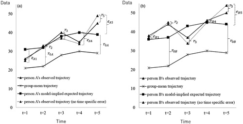
Time-specific errors ($r_1=1,r_2=-1,r_3=3,r_4=1$, and $r_5=-4$) can be observed by attending to the differences between the observed trajectories with and without time-specific errors. Importantly, while both random participant effects and residuals take different values between participants, participants are subjected to time-specific errors to the same extent. Specifically, in Figure 1a and 1b, the differences between the observed trajectories with and without time-specific errors are identical between participants. For example, at t = 3, trajectories with time-specific errors are 3 units larger than those without time-specific errors ($r_3=3$), and this pattern is consistent for both participants. This indicates that there may have been one or more sources that positively influenced both participants (e.g., the day of the assessment was payday or weekend). Similarly, at t = 5, observed trajectories with time-specific errors are 4 units smaller ($r_5=-4$) than those without time-specific errors, and this pattern is consistent for both participants. This indicates that there may have been sources that negatively influenced both participants (e.g., the day of the assessment was rainy or Monday).

Consequences of unmodeled time-specific errors

Underestimation of standard errors in estimating linear effect

The most significant consequence of the failure to incorporate time-specific errors in GCM is that it would cause considerable underestimation of standard errors of fixed effect estimates (e.g., linear slope effect), resulting in the inflation of type-1 error rates. The fact that unmodeled random effects increase type-1 error rates is not new. Clark (1973) raised the issue nearly 40 years ago in the field of psycholinguistics, and it has recently attracted revived attention in multiple fields of psychology (Baayen, Davidson, & Bates, 2008; Freeman, Heathcote, Chalmers, & Hockley, 2010; Judd, Westfall, & Kenny, 2012, Judd, Westfall, & Kenny, 2017; Murayama, Sakaki, Yan, & Smith, 2014). A similar issue has been discussed in the literature on multilevel modeling in the context of cross-classified models (Meyers & Beretvas, 2006; Rasbash & Browne, 2001; Raudenbush & Bryk, 2002). To our knowledge, however, this issue has been little discussed in longitudinal designs where various sources of time-specific errors may affect estimates in models including GCM. Given the popularity of GCM, this situation is rather surprising.

To illustrate the impact of time-specific errors on type-1 error rates of fixed effect estimates γ₁ in a simple manner, here we will assume ${\sigma }_1^2$ (random participant slopes) is zero. Under this model specification, from Equations (5)–(7), Y_jt can now be rewritten through the combined form as: (8) $$Y_{jt}=({\gamma }_0+{\gamma }_1{X}_t)+(u_{0j}+r_t+e_{jt}).$$(8)

From this equation, it is clear that the conditional variance of Y_jt at each timepoint can be expressed as (9) $$Var\left(Y_{jt}\right|X_t)={\sigma }_0^2+{\sigma }_t^2+{\sigma }_e^2={\sigma }^2,$$(9) because of independence among error terms (i.e., u_0j, r_t, and e_jt). Here, the variance is denoted as $Var()$. Similarly, conditional covariance between Y_jt and $Y_{jt\prime }$ (i.e., covariance between outcomes within the same participants), and covariance between Y_jt and $Y_{j\prime t}$ (i.e., covariance between outcomes within the same timepoints) are expressed as: (10) $$Cov(Y_{jt},Y_{jt\prime }|X_t,X_{t\prime })={\sigma }_0^2,$$(10) and (11) $$Cov(Y_{jt},Y_{j\prime t}|X_t)={\sigma }_t^2,$$(11) respectively. The covariance is denoted as $Cov()$.

We can now define an index which is analogous to the intra-class correlation coefficient (ICC) among outcomes within the same participants as follows: (12) $${\rho }_0=\mathit{\text{Corr}}(Y_{jt},Y_{jt\prime }|X_t,X_{t\prime })=\frac{{\sigma }_0^2}{{\sigma }_0^2+{\sigma }_t^2+{\sigma }_e^2}=\frac{{\sigma }_0^2}{{\sigma }^2},$$(12) and a similar index among outcomes within the same timepoints can be written as (13) $${\rho }_t=\mathit{\text{Corr}}(Y_{jt},Y_{j\prime t}|X_t)=\frac{{\sigma }_t^2}{{\sigma }_0^2+{\sigma }_t^2+{\sigma }_e^2}=\frac{{\sigma }_t^2}{{\sigma }^2}.$$(13)

The correlation is denoted as $\mathit{\text{Corr}}()$. These indices also express the proportion of variance explained by associated random factors. In the following discussion, without loss of generality, we set ${\gamma }_0=0$ (i.e., overall mean of outcome at t = 1 equal to 0) and ${\sigma }^2=1$ (i.e., variances of outcome at each timepoint equal to 1), respectively. Under this assumption, ${\rho }_0={\sigma }_0^2$ and ${\rho }_t={\sigma }_t^2$.

Let us illustrate the adverse effect of unmodeled time-specific errors. When both the values of ρ₀ and ρ_t are known and we use the GCM that correctly specified time-specific errors (i.e., Equations (5)–(7)), the statistic Z for testing a null hypothesis $H_0:{\gamma }_1=0$ (i.e., overall mean of slope is 0 with assuming ${\sigma }_1^2=0$) can be constructed as: (14) $$Z=\frac{{\widehat{\gamma }}_1}{se\left({\widehat{\gamma }}_1\right)}.$$(14)

A standard error of ${\widehat{\gamma }}_1$ is denoted as $se({\widehat{\gamma }}_1)$. Now, let $se({\widehat{\gamma }}_{1mis})$ be a standard error of the estimate of overall slope mean when we wrongly used the standard GCM (i.e., Equations (1)–(3) with assuming ${\sigma }_1^2=0$) but time-specific errors actually exist (i.e., ${\rho }_t={\sigma }_t^2>0$). The analytic formulas for $se({\widehat{\gamma }}_1)$ and $se({\widehat{\gamma }}_{1mis})$ can be found in the Online Supporting Materials. Under the conditions of ${\rho }_t\ge 0$, ${\rho }_0\ge 0,N\ge T\ge 1$, the following relation (15) $$se\left({\widehat{\gamma }}_{1mis}\right)\le se\left({\widehat{\gamma }}_1\right),$$(15) is always satisfied. In other words, a wrong use of the standard GCM that ignores time-specific errors always underestimates the standard error of overall slope mean estimates when time-specific errors actually exist. Note that expected values of ${\widehat{\gamma }}_1$ and ${\widehat{\gamma }}_{1mis}$ are equal, namely, $E({\widehat{\gamma }}_1)=E({\widehat{\gamma }}_{1mis})={\gamma }_1$, when the variance components (e.g., ρ₀ and ρ_t) are known (see Online Supporting Materials). This means that the failure to incorporate time-specific errors (when they are present) only impacts the standard error estimates of the linear slope, not (the expected value of) the linear slope estimate itself. However, when the variance components are unknown and T is small, there is a risk of substantial bias of slope estimates (see the general discussion below and footnote 7).

We describe the ratio $\frac{se({\widehat{\gamma }}_{1mis})}{se({\widehat{\gamma }}_1)}$ ($\le 1$) as shrinkage factor because this quantifies the degree of the underestimation of standard errors, through which the Z statistic in Equation (14)(14) $$Z=\frac{{\widehat{\gamma }}_1}{se\left({\widehat{\gamma }}_1\right)}.$$(14) inflates, which in turn inflates type-1 error. The analytic formulas of shrinkage factor are also shown in Online Supporting Materials. To examine the impact of the number of participants (N), the number of timepoints (T), the magnitude of the random participant intercepts (ρ₀), and the magnitude of time-specific errors (ρ_t) on the underestimation of standard errors we computed the shrinkage factor $\frac{se({\widehat{\gamma }}_{1mis})}{se({\widehat{\gamma }}_1)}$ and corresponding (inflated) type-1 error rates as a function of these parameter values. Specifically, we tabulated the shrinkage factor and corresponding type-1 error rates in Table 1 by systematically changing the number of participants (N = 200, 500, and 1,500), the number of timepoints (equally spaced, T = 5, 10, and 15), the proportion of variance explained by random participant intercept (ρ₀=0.2, 0.5, and 0.8), and the proportion of variance explained by time-specific errors (ρ_t=0, 0.01, 0.03, and 0.05). We selected these values because the variance of time-specific errors is likely to be substantially smaller than the variance of random participant intercepts (i.e., individual differences among participants).

Table 1. Shrinkage factor (and type-1 error rates) in the test of fixed coefficient for the linear term when we apply linear GCM without time-specific errors.

		T = 5			T = 10			T = 15
${\rho }_0$	${\rho }_t$	N = 200	N = 500	N = 1500	N = 200	N = 500	N = 1500	N = 200	N = 500	N = 1500
0.2	0.0	1 (0.05)	1 (0.05)	1 (0.05)	1 (0.05)	1 (0.05)	1 (0.05)	1 (0.05)	1 (0.05)	1 (0.05)
0.2	0.01	0.61 (0.23)	0.45 (0.38)	0.28 (0.59)	0.64 (0.21)	0.48 (0.35)	0.31 (0.55)	0.65 (0.20)	0.49 (0.33)	0.32 (0.53)
0.2	0.03	0.41 (0.42)	0.28 (0.59)	0.17 (0.75)	0.45 (0.38)	0.31 (0.55)	0.19 (0.72)	0.46 (0.36)	0.32 (0.53)	0.20 (0.70)
0.2	0.05	0.33 (0.51)	0.22 (0.67)	0.13 (0.80)	0.37 (0.47)	0.25 (0.63)	0.15 (0.78)	0.38 (0.45)	0.26 (0.61)	0.16 (0.76)
0.5	0.0	1 (0.05)	1 (0.05)	1 (0.05)	1 (0.05)	1 (0.05)	1 (0.05)	1 (0.05)	1 (0.05)	1 (0.05)
0.5	0.01	0.55 (0.28)	0.40 (0.43)	0.26 (0.62)	0.54 (0.29)	0.41 (0.42)	0.27 (0.59)	0.53 (0.30)	0.40 (0.43)	0.28 (0.59)
0.5	0.03	0.37 (0.47)	0.25 (0.62)	0.15 (0.76)	0.38 (0.45)	0.27 (0.59)	0.17 (0.74)	0.38 (0.46)	0.27 (0.59)	0.17 (0.73)
0.5	0.05	0.30 (0.55)	0.20 (0.69)	0.12 (0.82)	0.32 (0.53)	0.22 (0.67)	0.13 (0.80)	0.32 (0.54)	0.22 (0.66)	0.14 (0.79)
0.8	0.0	1 (0.05)	1 (0.05)	1 (0.05)	1 (0.05)	1 (0.05)	1 (0.05)	1 (0.05)	1 (0.05)	1 (0.05)
0.8	0.01	0.37 (0.47)	0.27 (0.60)	0.17 (0.73)	0.36 (0.49)	0.26 (0.61)	0.18 (0.73)	0.34 (0.50)	0.25 (0.62)	0.17 (0.73)
0.8	0.03	0.24 (0.64)	0.17 (0.74)	0.10 (0.84)	0.24 (0.64)	0.17 (0.74)	0.11 (0.83)	0.23 (0.66)	0.17 (0.75)	0.11 (0.83)
0.8	0.05	0.19 (0.71)	0.13 (0.80)	0.08 (0.88)	0.19 (0.71)	0.13 (0.80)	0.08 (0.87)	0.18 (0.72)	0.13 (0.80)	0.08 (0.87)

T: number of (equally spaced) timepoints; N: number of participants; ${\rho }_0$: proportion of variance explained by random participant intercept factor; ${\rho }_t$: proportion of variance explained by time-specific error.

The results showed that (i) even the small sizes of ρ_t (e.g., ${\rho }_t=.01$) dramatically underestimate standard error estimates (estimated standard errors are sometimes less than 1/5 of the true standard errors) and cause serious inflation of type-1 error rates, (ii) large N also underestimates standard errors (and causes inflation of type-1 error rates), whereas large T generally prevents this but its impact is much smaller as compared with N, and (iii) when time-specific errors (ρ_t) are present, larger ρ₀ also leads to larger underestimation of standard error estimates and more serious inflation of type-1 error rates. When ${\rho }_t=0$, however, standard errors and type-1 error rates are correctly estimated (i.e., shrinkage factor =1).

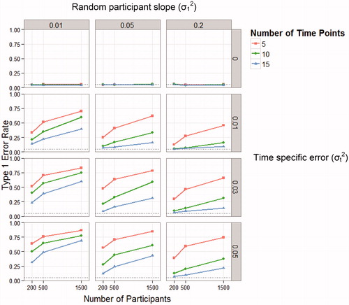
The analyses presented here are limited in that they assumed (1) there are no random participant slopes (i.e., ${\sigma }_1^2=0$) and (2) the variance components (e.g., ρ₀ and ρ_t) are known. To support the generalizability of our argument and to illustrate how the underestimated standard errors impact actual type-1 error rates, we conducted Monte Carlo simulations under the conditions where random participants’ slopes are present and computed empirical type-1 error rates. In these simulations, a linear GCM with time-specific errors (i.e., Equations (5)–(7), with fixing ${\gamma }_1=0$) was used as a data generation model but the standard linear GCM (i.e., Equations (1)–(3) was (wrongly) fit to the data. We systematically changed the number of participants (N = 200, 500, and 1,500), the number of timepoints (equally spaced, T = 5, 10, and 15), the magnitude of time-specific errors (${\sigma }_t^2$= 0, 0.01, 0.03, and 0.05), and the magnitude of random participant slope (${\sigma }_1^2$= 0.01, 0.05, and 0.20). We fixed the magnitude of random participant intercept ${\sigma }_0^2$ to 0.5 and specified residual variance ${\sigma }_e^2$ as ${\sigma }_e^2=1-{\sigma }_t^2-{\sigma }_0^2$. For each combination of simulation parameters, 1,000 data sets were generated and simulated type-1 error rates were evaluated by computing the proportion of significant (false-positive) effects of regression slope (i.e., ${\widehat{\gamma }}_1$) with α = 0.05. In this simulation, all analyses that apply the mixed-effects models were performed using restricted maximum likelihood by the lme4 package in R. (Bates, Maechler, & Bolker, 2011).

The results of Figure 2 were consistent with the observations in Table 1. Specifically, even with small time-specific errors (e.g., ${\rho }_t<0.01$) type-1 error rates considerably increase (sometimes above 50%), and larger N increase type-1 error rates, whereas a larger T decreases type-1 error rates.⁴ Difference from Table 1 can be seen in that T has larger impact on type-1 error rates.

Figure 2. Type-1 error rates of fixed linear slope as a function of number of participants and number of timepoints, when time-specific errors are not included in growth curve model. The predetermined alpha value (α = 0.05) is highlighted by the dotted line.

Underestimation of standard errors in estimating quadratic effect

In many applications of GCM, linear slope is obviously nonzero (e.g., GCM to evaluate the growth trajectories of height of children), and therefore the inflation of type-1 error rates for the linear slope effect may not be a serious issue. The issue is relevant, however, when it comes to the statistical tests of quadratic effects. We are often interested in determining the shape of a growth curve, and for that purpose, we typically include a quadratic term in a linear GCM to test the nonlinearity of the growth curve (e.g., Bollen & Curran, 2006; McArdle & Nesselroade, 2014; Ram & Grimm, 2015). Importantly, like linear slope effect, time-specific errors would artificially reduce the standard error of this nonlinear effect estimate when time-specific errors are not appropriately modeled (i.e., GCM of Equations (5)–(7) is not used), resulting in a substantial inflation of type-1 error rates. This inflation is of more serious concern in practice, not only because this means that researchers would wrongly identify the shape of the growth curve but also because the misspecified quadratic term would influence the estimate of overall slope and its differences among participants. If researchers want to include an independent variable to predict participant slopes, for example, the presence or absence of quadratic term would make a difference (Biesanz, Deeb-Sossa, Papadakis, Bollen, & Curran, 2004; Bollen & Curran, 2006).

To illustrate how time-specific errors influence standard error estimates of a quadratic term, consider the following model: (16) $$Y_{jt}={\beta }_{0j}+{\beta }_{1j}{X}_t+{\beta }_{2j}{X}_t^2+(r_t+e_{jt}),$$(16) where (17) $${\beta }_{0j}={\gamma }_0+u_{0j},$$(17) (18) $${\beta }_{1j}={\gamma }_1+u_{1j},$$(18) (19) $${\beta }_{2j}={\gamma }_2+u_{2j}.$$(19)

γ₂ is the overall mean of the slope expressing quadratic change, and u_2j is a corresponding random slope of participants. u_2j is assumed to be independent of predictors X_t and other residuals and random factors. $u_{0j},u_{1j}$, and u_2j are assumed to follow a multivariate normal distribution, taking a form analogous to Equation (4)(4) $$\left(\begin{array}{c}{u}_{0j}\\ u_{1j}\end{array}\right)\sim N\left(\left(\begin{array}{c}0\\ 0\end{array}\right),\left(\begin{array}{cc}{\sigma }_0^2& {\sigma }_{01}\\ {\sigma }_{01}& {\sigma }_1^2\end{array}\right)\right).$$(4) . To simplify, only random participant intercept u_0j (i.e., ${\sigma }_0^2$) is considered here and other random participant effects $u_{1j}$ and u_2j are fixed to zero (i.e., $u_{1j}$=u_2j=0 for all j).

In this case, the combined form of the model is: (20) $$Y_{jt}=({\gamma }_0+{\gamma }_1{X}_t+{\gamma }_2{X}_t^2)+(u_{0j}+r_t+e_{jt}).$$(20)

Let ${\widehat{\gamma }}_{1mis}$ and ${\widehat{\gamma }}_{2mis}$ be parameter estimates of slopes for linear and quadratic changes when the standard quadratic GCM is wrongly fit to the data (i.e., setting r_t = 0 for all t in Equation (20)(20) $$Y_{jt}=({\gamma }_0+{\gamma }_1{X}_t+{\gamma }_2{X}_t^2)+(u_{0j}+r_t+e_{jt}).$$(20) ). Mathematical derivations of shrinkage factors $se({\widehat{\gamma }}_{1mis})/se({\widehat{\gamma }}_1)$ and $se({\widehat{\gamma }}_{2mis})/se({\widehat{\gamma }}_2)$ can be found in the Online Supporting Materials. Under the conditions of ${\rho }_t\ge 0$, ${\rho }_0\ge 0,N\ge T\ge 1$, the following relations are always satisfied: (21) $$se\left({\widehat{\gamma }}_{1mis}\right)\le se\left({\widehat{\gamma }}_1\right),se\left({\widehat{\gamma }}_{2mis}\right)\le se\left({\widehat{\gamma }}_2\right),$$(21)

These results indicate that the incorrect use of the standard GCM, which ignores time-specific errors, always underestimates the standard errors associated with both coefficient estimates for the linear and quadratic terms.

Table 2 provides the computed shrinkage factors (i.e., $\frac{se({\widehat{\gamma }}_{2mis})}{se({\widehat{\gamma }}_2)}$) and corresponding type-1 error rates for the coefficient of the quadratic term, as a function of the number of participants (N), the number of timepoints (T), the magnitude of random participant intercepts (ρ₀), and the magnitude of time-specific errors (ρ_t). The table for the linear slope (i.e., $\frac{se({\widehat{\gamma }}_{1mis})}{se({\widehat{\gamma }}_1)}$ and corresponding type-1 error rates) is not presented, but available upon request to the corresponding author. This table indicates similar underestimation patterns of the standard error estimates with those of the linear slope in Table 1 – the existence of ρ_t causes substantial underestimation of the standard error, and this underestimation is exacerbated by increasing N. Again, T does not have a big impact on the shrinkage factor, and ρ₀ is influential when ρ_t and N are small. These findings highlight the risk of drawing incorrect conclusions about the shape of the growth trajectories and overall slope if researchers fit the standard GCM without considering the presence of time-specific errors. We also conducted Monte Carlo simulations under conditions where random participants’ effects for the coefficients of the slope terms are present. In these simulations, a quadratic GCM with time-specific errors (i.e., Equations (16)–(19), with fixing ${\gamma }_2=0$ and $u_{2j}=0$) was used for the data generation model but the standard quadratic GCM without time-specific errors (i.e., setting $u_{2j}=0$ and r_t=0 for all t) was wrongly fit to the data. The linear slope was fixed to a positive constant (${\gamma }_1=0.2$), and parameters of the data generation model were systematically changed as done with the previous simulations of linear slope. For each combination of simulation parameters, 1,000 data sets were generated. Again, the results (Figure S1 in Online Supporting Materials) were consistent with the observations in Table 2, confirming the generalizability of the findings.

Table 2. Shrinkage factor (and type-1 error rates) in the test of fixed coefficient for the quadratic term when we apply quadratic GCM without time-specific errors.

		T = 5			T = 10			T = 15
${\rho }_0$	${\rho }_t$	N = 200	N = 500	N = 1500	N = 200	N = 500	N = 1500	N = 200	N = 500	N = 1500
0.2	0.0	1 (0.05)	1 (0.05)	1 (0.05)	1 (0.05)	1 (0.05)	1 (0.05)	1 (0.05)	1 (0.05)	1 (0.05)
0.2	0.01	0.55 (0.28)	0.39 (0.45)	0.24 (0.64)	0.57 (0.26)	0.40 (0.43)	0.25 (0.63)	0.58 (0.25)	0.41 (0.42)	0.26 (0.62)
0.2	0.03	0.36 (0.48)	0.24 (0.64)	0.14 (0.79)	0.37 (0.46)	0.25 (0.63)	0.15 (0.77)	0.38 (0.45)	0.26 (0.62)	0.15 (0.77)
0.2	0.05	0.28 (0.58)	0.18 (0.72)	0.11 (0.83)	0.30 (0.56)	0.19 (0.70)	0.11 (0.82)	0.31 (0.55)	0.20 (0.69)	0.12 (0.82)
0.5	0.0	1 (0.05)	1 (0.05)	1 (0.05)	1 (0.05)	1 (0.05)	1 (0.05)	1 (0.05)	1 (0.05)	1 (0.05)
0.5	0.01	0.48 (0.35)	0.33 (0.52)	0.20 (0.70)	0.50 (0.33)	0.35 (0.49)	0.21 (0.67)	0.50 (0.32)	0.36 (0.48)	0.22 (0.66)
0.5	0.03	0.30 (0.55)	0.20 (0.70)	0.12 (0.82)	0.32 (0.53)	0.21 (0.68)	0.13 (0.81)	0.33 (0.52)	0.22 (0.67)	0.13 (0.80)
0.5	0.05	0.24 (0.64)	0.15 (0.76)	0.09 (0.86)	0.25 (0.62)	0.17 (0.75)	0.10 (0.85)	0.26 (0.61)	0.17 (0.74)	0.10 (0.84)
0.8	0.0	1 (0.05)	1 (0.05)	1 (0.05)	1 (0.05)	1 (0.05)	1 (0.05)	1 (0.05)	1 (0.05)	1 (0.05)
0.8	0.01	0.33 (0.52)	0.22 (0.67)	0.13 (0.80)	0.34 (0.51)	0.23 (0.65)	0.14 (0.78)	0.34 (0.51)	.23 (0.65)	0.15 (0.78)
0.8	0.03	0.19 (0.70)	0.13 (0.81)	0.07 (0.89)	0.21 (0.69)	0.14 (0.79)	0.08 (0.87)	0.21 (0.68)	0.14 (0.78)	0.08 (0.87)
0.8	0.05	0.15 (0.78)	0.09 (0.85)	0.05 (0.92)	0.16 (0.76)	0.10 (0.84)	0.06 (0.91)	0.16 (0.75)	0.10 (0.84)	0.06 (0.90)

T: number of (equally spaced) timepoints; N: number of participants; ${\rho }_0$: proportion of variance explained by random participant intercept factor; ${\rho }_t$: proportion of variance explained by time-specific error.

Note that even when the proposed GCM that assumes different functional forms (e.g., cubic GCM) is applied, the presence of time-specific error variances (i.e., covariances between participants within each timepoint) leads to the similar results. In other words, if time-specific errors are present and if T by T covariance structure among timepoints (${\mathbf{\Sigma }}^{*}$) is positive definite, standard errors of slope coefficients estimates in the proposed GCM become larger than those in the standard GCM (see also Online Supporting Materials).

Effectiveness of the proposed model to prevent the inflation of type-1 errors

To demonstrate the effectiveness of the proposed mixed-effects models, we ran another set of Monte Carlo simulations. These simulations confirmed that the proposed GCMs can effectively address the inflation of type-1 error rates when they are applied to the data generated from a linear GCM and quadratic GCM with and without time-specific errors (Figure S2 and S3 in Online Supporting Materials) and that the proposed GCMs can effectively recover true parameters without bias (Table S1 in Online Supporting Materials).

Notes on time-specific errors

Covariance structure of the proposed model

To clarify the implications of time-specific errors, let us consider the covariance structure of the proposed GCM. For example, when T = 3 and N = 2 in the proposed linear GCM, from the Equations (8)–(11) mean structure $\mathit{\mu }$ and covariance structure $\mathbf{\Sigma }$ for $\mathit{Y}=(Y_{11},Y_{12},Y_{13},Y_{21},Y_{22},Y_{23})\prime$ can be expressed as (see Online Supporting Materials for general expressions): (22) $$\mathit{\mu }=({\gamma }_0,{\gamma }_0+{\gamma }_1,{\gamma }_0+2{\gamma }_1,{\gamma }_0,{\gamma }_0+{\gamma }_1,{\gamma }_0+2{\gamma }_1)\prime ,$$(22) and (23) $$\mathbf{\Sigma }=\left(\begin{array}{cccccc}{\sigma }^2& {\sigma }_0^2& {\sigma }_0^2& {\sigma }_t^2& 0& 0\\ {\sigma }_0^2& {\sigma }^2& {\sigma }_0^2& 0& {\sigma }_t^2& 0\\ {\sigma }_0^2& {\sigma }_0^2& {\sigma }^2& 0& 0& {\sigma }_t^2\\ {\sigma }_t^2& 0& 0& {\sigma }^2& {\sigma }_0^2& {\sigma }_0^2\\ 0& {\sigma }_t^2& 0& {\sigma }_0^2& {\sigma }^2& {\sigma }_0^2\\ 0& 0& {\sigma }_t^2& {\sigma }_0^2& {\sigma }_0^2& {\sigma }^2\end{array}\right).$$(23)

Like standard multilevel models, observations within the same participants are correlated with each other (${\sigma }_0^2$). Most importantly, in the proposed GCM with time-specific errors, ${\sigma }_t^2$ appears in the covariance between persons within the same timepoints. This feature means that time-specific errors produce the correlations between persons within the same timepoints after controlling for fixed effects. In other words, the proposed GCM (with time-specific errors) allows data from different participants within each timepoint to be correlated. In standard GCM, on the other hand, participants are posited to be independent from each other (after accounting for fixed effects).

Comparison with other models

Although this article specifies GCMs with a multilevel modeling framework (or mixed-effects model; Goldstein, 2003; Raudenbush & Bryk, 2002; Singer & Willett, 2003), time-specific errors are a more general issue that also apply to the GCMs specified by the structural equation modeling (SEM) framework using a restricted common factor model (McArdle, Anderson, Birren, & Schaie, 1990; Meredith & Horn, 2001). Unfortunately, it is not easy to effectively incorporate time-specific errors in the SEM framework, as standard (single-level) SEM addresses the variance/covariance between timepoints (i.e., variables) only, but not between participants. Although it is not impossible to consider covariance between participants (see Mehta & Neale, 2005), this involves substantial procedural and conceptual difficulties. On the other hand, the proposed GCM, which is based on a cross-classified model (rather than SEM framework), should provide a more direct and flexible way to account for possible time-specific errors. Thus, we strongly recommend specifying the model with a mixed-effects model rather than with the SEM framework.

Some may argue that researchers can also treat time as a categorical variable, without using the proposed GCM. Namely, we can capture time-specific errors at each specific time by including T – 1 fixed-effects (dummy codes) for time using the standard GCM. Alternatively, we can also add time-varying additive constants to represent time-specific effects. These specifications have a close relationship with latent basis growth model (Ram & Grimm, 2015; or a free factor loadings approach; Bollen & Curran, 2006. i.e., treating X_t as parameters to be estimated rather than fixed constants, beside minimal constraints needed for model identification). This method is also similar with a traditional repeated-measures analysis of variance (ANOVA) with time as a fixed repeated measurement factor. These models determine the growth curves in a data-driven manner; thus, all of these models can capture any idiosyncratic growth curves present in the data, including growth curves with time-specific errors. However, these methods are inappropriate in that time-specific influences are treated as fixed effects rather than random ones. Furthermore, importantly, these methods cannot disentangle time-specific influences from the true latent trajectory, making it impossible to estimate true growth curves dissociated from time-specific errors. This means that these models cannot evaluate the trend of growth trajectory (e.g., linear and quadratic) and parameter estimates would be difficult to map onto theoretical notion of the development and growth processes (Ram & Grimm, 2015).

In the literature of psychometrics, econometrics, and other related fields, there are many longitudinal models proposed with SEM or time-series modeling frameworks to account for time-specific effects. The examples include the autoregressive latent trajectory (ALT) model with time-varying autoregressive parameters (Bollen & Curran, 2004; Curran & Bollen, 2001), the unified latent curve, latent state-trait model (LC-LSTM) (Alessandri, Caprara, & Tisak, 2012), statistical models for intensive longitudinal data (Walls & Schafer, 2006; Hamaker, Ceulemans, Grasman, & Tuerlinckx, 2015), unconditional asset pricing models (Shanken, 1990), stochastic time-varying coefficient models (Giraitis, Kapetanios, & Yates, 2014), time-varying vector autoregressive (VAR) models (Primiceri, 2005), and time-varying effect models (TVEM) (Shiyko, Lanza, Tan, Li, & Shiffman, 2012). Using the SEM framework, GCM has also been extended to fit various types of growth curves, such as latent basis growth model and GCM with exponential growth curves (Grimm, Ram, & Hamagami, 2011; Grimm, Steele, Ram, & Nesselroade, 2013; see also Preacher & Hancock, 2015 for general expression). These models are seemingly similar with our proposed model in that they incorporate time-varying effects (e.g., random participants effects in changes) in some way, but our proposed model is different from these models in how time-varying effects are defined. None of the models above incorporate random errors which vary across timepoints but are constant across participants within given timepoints (i.e., time-specific errors). More detailed discussion on this point is provided in the Online Supporting Materials.

Other potential solutions by research design

There are several ways to reduce time-specific errors. One effective design is to assess participants at different timepoints (i.e., timepoints are nested within, rather than crossed with, participants), such as a standard experience sampling method where participants answer questions at random intervals (Bolger, Davis, & Rafaeli, 2003). In a nested design, we cannot estimate time-specific errors because this design does not allow us to compute any time-specific effects that influence all participants. However, because no one shares the common measurement timepoints, conflation of time-specific errors (r_t) and residual (e_jt) do not cause underestimation of standard errors of growth parameter estimates. In other words, time-specific errors do not inflate type-1 error rates in a nested design. We can also reduce the impact of time-specific errors using longitudinal data that are partly crossed (i.e., data of some participants are measured at the same timepoints), and we can still apply the proposed GCM if necessary.

Collection and inclusion of time-varying covariates should also be useful to reduce the influence of time-specific errors. In the example of assessing employees’ morale in organizations, if researchers consider that the day and economic conditions are sources of time-specific errors, gathering the information regarding the day and diffusion index at each assessment should be useful. Researchers can estimate growth curves that remove the effects of these covariates. Specifically, instead of specifying time-specific errors, researchers can include time-specific covariates ${\mathrm{Z}}_t$ to explain the outcome Y_jt as $Y_{jt}={\beta }_{0j}+{\beta }_{1j}{X}_t+{\sum }_p^{}{w}_p{Z}_{pt}+(r_t+e_{jt})$ (w_p is a partial regression coefficient for pth time-specific covariate Z_pt).

This strategy is similar with applications of multilevel modeling to reduce the influence of intra-class correlation on experimental effect estimates in cluster randomized trials (e.g., Hedges & Hedberg, 2007; Murray & Blistein, 2003; Usami, 2014). However, it is very difficult in practice to identify all sources of time-specific errors in advance and collect these covariates. In addition, even if all covariate information is available, there is still a risk of model misspecification (see the next section) and this causes failure to effectively account for time-specific errors in GCM. Therefore, inclusion of time-varying covariates is undoubtedly useful, despite not being an optimal strategy to address the problem of time-specific errors. The proposed GCM with time-specific errors, on the other hand, can capture all potential time-specific errors by a single parameter (${\sigma }_t^2$), providing a more parsimonious and practical solution to the problem.

The issue of model misspecification of the growth function and a potential solution

Artificial time-specific errors caused by model misspecification of the growth function

Although the proposed GCM has the ability to effectively account for time-specific errors that are not captured by existing models, there is one issue that researchers need to bear in mind – model misspecification. As Skrondal and Rabe-Hesketh (2004) noted, in reality we often analyze data based on a wrong model or untenable assumptions. This model misspecification can take a variety of forms, including omitted variables, inappropriate link functions, inappropriate variance functions, inappropriate distributional assumptions, and violation of conditional independence. Misspecified models can potentially lead to biased parameter estimates and misleading conclusions.

In the context of the proposed model with time-specific errors, one important model misspecification to consider is the misspecification of the functional form of the growth curve. For example, a researcher may fit a linear GCM to data, even if the true growth curve is nonlinear. Importantly, because time-specific errors essentially represent the deviation of observed trajectory from the growth trajectory implied from the model (Figure 1), when the linear model is wrongly specified and the shape of true latent trajectory is actually quadratic (i.e., nonlinear), time-specific errors in our proposed model could “soak up” this misspecification. Specifically, the model could account for temporal mean deviation from the implied growth curves that are similar for all participants at each timepoint. As a result, even in the absence of time-specific errors, the results may show a nonzero estimate of time-specific errors (i.e., ${\sigma }_t^2>0$), and the researcher may incorrectly claim that the true growth trajectory is linear. In this case, the larger the magnitude of parameters associated with quadratic slope (i.e., γ₂, ${\sigma }_2^2$) is, the risk of having a nonzero estimate of time-specific errors becomes greater. Of course, our proposed model with time-specific errors can be extended to incorporate nonlinear functions to alleviate the influence of model misspecification. However, although having a theory or substantive knowledge about the target construct and data collection process is of great help, it is almost impossible for researchers to know the exact shape of the true latent trajectory before analyzing data. To get an idea for the presence of time-specific errors, some exploratory analyses such as a scatterplot might be a useful strategy, especially when the number of timepoints (T) and time-specific error variances (${\sigma }_t^2$) are large (in the context of model misspecification, see Cudeck & Harring, 2007).

It should be noted that model misspecification is not an issue specific to our proposed model, but a general problem for GCM (Wu, West, & Taylor, 2009). Unless we know the true growth trajectory in advance, model misspecification can always occur in GCM. In addition, using a GCM with time-specific errors, model misspecification would result in the overestimation of standard errors, which makes the statistical test more conservative than GCMs without time-specific errors. Nevertheless, the issue of model misspecification is more of a concern in our proposed model because the “soaking up” property of GCM with time-specific errors can mask the potential misfit between the true and the model implied trajectories. Thus, we need to be careful when we obtain a large estimate of time-specific errors variance (${\sigma }_t^2$); we need to suspect a potential risk of model misspecification and need to consider what the obtained time-specific errors actually imply. In other words, relatively large time-specific error variance might indicate the possibility that time-specific errors are confounded with (unspecified) true growth trajectories due to model misspecification.

Serial correlations: a potential solution

One potential solution to detect model misspecification is to scrutinize the pattern of the residuals from the estimated latent trajectory (i.e., estimated residuals). If there is a model misspecification, these estimated residuals should show systematic patterns, yielding nonzero serial correlation of residuals across timepoints. For example, imagine that the shape of the true latent trajectory can be expressed by a quadratic form $y=10+t+t^2$ and observed means are 12, 16, 22, 30, and 40 from t = 1 to t = 5. A researcher wrongly applies a linear GCM to the data, and obtains an estimated growth trajectory, which indicates the estimated means of 10, 17, 24, 31, and 38 at each timepoint (i.e., the means of the intercept and linear change are estimated to be 10 and 7, respectively). In this case, the estimated residuals, calculated as the differences between the observed means and the model-implied (estimated) means, are 2, –1, –2, –1, and 2. These values suggest systematic patterns (i.e., a U-shaped pattern) that indicate nonzero serial correlation, implying the violation of the assumption of residuals (i.e., conditional independence of residuals).

In the present context, estimates of residuals ${\widehat{r}}_t$ can be obtained in the linear GCM with time-specific errors (i.e., Equations (5)–(7)) as (24) $${\widehat{r}}_t={\overline{Y}}_{.t}-({\widehat{\gamma }}_0+{\widehat{\gamma }}_1{X}_t),$$(24) and in the quadratic GCM with time-specific errors (i.e., Equations (16)–(19)) as (25) $${\widehat{r}}_t={\overline{Y}}_{.t}-({\widehat{\gamma }}_0+{\widehat{\gamma }}_1{X}_t+{\widehat{\gamma }}_2{X}_t^2).$$(25)

Here, ${\overline{Y}}_{.t}=\sum Y_{jt}/N$ is the average of outcome at t. Let ${\widehat{r}}_{a,b}$ with $a\ge 1$ and $b\le T$ be ${\widehat{r}}_{a,b}=({\widehat{r}}_a,{\widehat{r}}_{a+1},\dots ,{\widehat{r}}_{b-1},{\widehat{r}}_b)\prime$. Then, first and second serial correlations can be estimated as (26) $$R_1=cor({\widehat{r}}_{1,T-1},{\widehat{r}}_{2,T}),R_2=cor({\widehat{r}}_{1,T-2},{\widehat{r}}_{3,T}),$$(26) respectively. See Appendix A for R codes to compute such residuals.

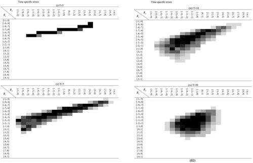
When we apply a GCM with time-specific errors, we can compute these serial correlations, and if either of these correlations is large, we suspect potential model misspecification. To provide a practical guideline of the magnitude of serial correlation, we evaluated the sampling distribution of these serial correlations using statistical simulation. We simulated the sampling distribution of serial correlations when time-specific errors ${\widehat{r}}_t$ are present and appropriately modeled. Using these sampling distributions, we can evaluate the possibility of model misspecification by checking whether observed serial correlations exhibit extreme values in the distribution. Using both linear and quadratic GCM with time-specific errors, the joint distribution of first and second serial correlations (R₁, R₂) is evaluated using 5,000 replications generated by a model with time-specific errors. We evaluated the joint sampling distribution by varying the number of timepoints T (=5, 6, 7, 8, 9, 10, 20, 50). Appendix B displays this joint distribution. All correlations are distributed into 20 bins (bin width =0.1), producing a total of 20 × 20 = 400 cells, and cells with larger frequencies are colored in darker shades. Cells that show frequencies lower than 10 are not colored because they are at high risk of sampling errors and are thus ignored (colored cells in tables of Appendix B include 94.8%–99.9% of the whole [=5,000] data). Note that first and second serial correlations cannot be evaluated unless $T\ge 4$ and $T\ge 5$, respectively.

From Appendix B, we can see some patterns in the shape of the joint distribution for T = 5, 7, 10, and 20. A larger T indicates higher density around the center of the distribution (i.e., no serial correlations, (R₁, R₂) = (0,0)). The first serial correlation generally shows smaller variance than the second serial correlation, and the second serial correlation shows wide distribution, especially when T is small (T = 5). Note that this sampling distribution is not influenced by N, ρ₀, and ρ_t, making this procedure particularly accessible and useful for applied researchers to detect potential model misspecification.⁵ If estimated serial correlations calculated from the proposed GCM with time-specific errors do not fall within the colored cells, in which the significance levels are approximately equal to or lower than 5%, we can conclude that the estimated (nonzero) time-specific errors may include artifacts caused by model misspecification.

Effectiveness of the solution

To empirically illustrate the effectiveness of the joint sampling distributions that we derived, we generated data from a quadratic (i.e., nonlinear) GCM without time-specific errors (i.e., Equations (16)–(19) with $u_{1j}=u_{2j}=r_t=0$, ${\gamma }_0=0,{\gamma }_1=1$, and ${\rho }_0=0.5$), and applied a linear GCM with time-specific errors (i.e., with a misspecified model). We systematically varied the number of timepoints (T = 5, 7, 10, and 20), number of sample sizes (N = 100 and 500), and the magnitude of the quadratic effect (${\gamma }_2=0.1,0.2$). In all, 200 simulation data sets were generated for each condition. In each condition, we examined whether the estimated serial correlations were outside of the colored cells in the joint sampling distribution we provided. Table 3 summarizes the proportion of cases when model misspecification was correctly identified. The results showed that, when T is small (i.e., T = 5), the proposed procedure with serial correlations does not detect model misspecification well. However, the proposed procedure works much better with T = 7 and can detect model misspecification very effectively when T > 7, especially when N is larger and the shape of the true latent trajectory deviated more from the linear trajectory (i.e., γ₂ is larger). These results indicate that the use of serial correlations can be an effective way to address the issue of model misspecification in GCMs with time-specific errors.

Table 3. Proportions that the estimated serial correlations do not fall within the colored cells shown in Figure B1 and B2, when a GCM with time-specific errors are wrongly fitted to the data generated from the quadratic GCM without time-specific errors (left). The proportions that information criteria correctly favored the quadratic GCM without time-specific errors (right).

		Serial correlations		AIC		BIC
		${\gamma }_2=0.1$	${\gamma }_2=0.2$	${\gamma }_2=0.1$	${\gamma }_2=0.2$	${\gamma }_2=0.1$	${\gamma }_2=0.2$
N = 100	T = 5	0	0	0.82	0.98	0.82	0.98
	T = 7	0.77	0.96	0.99	1	0.99	1
	T = 10	1	1	1	1	1	1
	T = 20	1	1	1	1	1	1
N = 500	T = 5	0	0	0.93	1	0.93	1
	T = 7	0.97	1	1	1	1	1
	T = 10	1	1	1	1	1	1
	T = 20	1	1	1	1	1	1

T: number of (equally spaced) timepoints. N: number of participants.

AIC: Akaike Information Criteria. BIC: Bayesian Information Criteria.

In GCM, we sometimes evaluate potential model misspecification using model selection methods such as information criteria when alternative models are available. Thus, in the simulation reported above, we also evaluated the utility of information criteria using Akaike information criterion (AIC) and Bayesian information criterion (BIC). We compared the information criteria between (a) when we applied a quadratic GCM without time-specific errors (i.e., true model) and (b) when we applied a linear GCM with time-specific errors (i.e., misspecified model). The results (Table 3) showed that both information criteria successfully selected the true model in most of the conditions. These results indicate that, when researchers are aware of potential alternative models that can explain the growth curve without time-specific errors, information criteria can be useful to detect potential model misspecification, especially in conjunction with serial correlations. It should be noted that serial correlations are only useful when model misspecification comes from the shape of the latent trajectory (i.e., functional form of growth curves). However, this is not the only form of model misspecification in GCM (Skrondal & Rabe-Hesketh, 2004; Wu et al., 2009). For example, the true model can be different to a model with time-specific errors in terms of the assumptions of distribution and variance. In such a situation, the use of information criteria such as AIC and BIC would be of particular value, if alternative models are available.

A flowchart to treat time-specific errors and real data example

As a summary of the discussion so far, we provide a flowchart below so that applied researchers can know how to deal with time-specific errors step-by-step.

1. Using substantial knowledge of previous empirical findings and data, consider whether there are potential sources of time-specific errors (i.e., errors which change randomly across timepoints but cause measurement biases for all participants within timepoints). Exploratory data analysis (e.g., scatterplot) and substantive theory might help to detect the presence of the time-specific errors. If the researcher suspects the presence of time-specific errors, move onto the next step (or, apply the standard GCM or some longitudinal models if not).

2. Think about a design that can mitigate the effects of time-specific errors (e.g., sample different timepoints across participants so that time is nested within, rather than crossed with, participants; collect time-specific covariates). If it is difficult to implement such a design or the researcher suspects that time-specific errors are still present even with such design, use the proposed GCM that incorporates time-specific errors.

3. If estimated time-specific errors variance (${\sigma }_t^2$) is statistically significant, calculate serial correlations.

4. If estimated serial correlations do not fall within the colored cells in the joint distribution (provided in Appendix B), the estimated (nonzero) time-specific errors may include artifacts caused by model misspecification. In this case, researchers should consider alternative longitudinal models to fit data. If estimated serial correlations fall within the colored cells, results from the proposed GCM with time-specific errors should be used.

If there are multiple competing GCMs that have nested relationships with each other (e.g., linear GCM and quadratic GCM) to fit the data in step 2, applying the GCM that assumes more generalized functional form (e.g., quadratic GCM) first might be reasonable in many situations because it can decrease the risk of model misspecification of functional form.

To illustrate how we can deal with time-specific errors, we present an example with real data using data from Tanaka and Murayama (2014). In the analyses provided below, we estimated parameters using restricted maximum likelihood by the lme4 package in R (Bates et al., 2011). Tanaka and Murayama (2014) longitudinally assessed students’ interest in an introductory psychology class over a semester, which comprised 12 weeks of classes (T = 12). From weeks 1 through 12, all participants responded to questionnaires on their motivation after each class. Thus, participants are crossed with timepoints in the data. The average scores for two items (“Today’s class was interesting”; “I like today’s class”) from studies by Wigfield and Eccles (2000) and Eccles and Wigfield (1995) were used to calculate an interest index (index range: 1–5). Due to attrition and absence, out of all observations 22.7% were not observed in this dataset.⁶ Each class was generally self-contained, addressing different topics of psychology.

The primary purpose of the paper was not to examine the longitudinal trajectory of students’ interest level, so consequently, Tanaka and Murayama (2014) did not use GCM in the paper. However, we will now fit GCMs to the data for illustrative purposes. We provide the data set and corresponding codes of R, SPSS, and SAS in the Online Supporting Material. There has been accumulating evidence in educational psychology that students’ motivation at schools declines over years, indicating the difficulty in sustaining motivation over a long time frame (e.g., Fredricks & Eccles, 2002; Frenzel, Goetz, Pekrun, & Watt, 2010). By applying GCM to the current data, we can examine whether we can observe the same pattern of decline even within a shorter time frame (i.e., over a semester).

In this particular example, one plausible source of time-specific errors is the content of the topics that are covered right before the assessment points. It is possible that participants’ interest would be generally enhanced after they were taught a more interesting topic, or the class was more engaging than usual. It is also possible that participants’ interest would generally drop when the content was dull. For the purpose of examining the general longitudinal trend of interest (i.e., “Does interest generally decline over time?”), these factors are confounds when trying to estimate true growth curves. Because these sources are considered to change randomly between timepoints and influence all participants, it is worth considering the application of the proposed GCM to the data (Step 1).

The results are summarized in Table 4. For illustrative purposes, we fit separate GCMs without and with time-specific errors. When we applied a standard quadratic GCM (without time-specific errors) with random participant intercepts and linear slopes (time coding was anchored at the initial assessment point; Biesanz et al., 2004), both linear and quadratic effects exhibited statistical significance, ${\widehat{\gamma }}_1$ = 0.08, $t(1655)=2.59$, p < .05; ${\widehat{\gamma }}_2$ = –0.01, $t(1517)=3.21$, p < .05. These results indicate that students’ interest level increased at the beginning but started to drop off in the middle of the course.

Table 4. GCM with and without time-specific errors for the data from Tanaka and Murayama (2014).

	Without time-specific errors	With time-specific errors
Fixed effects (standard errors)
Intercept (γ0)	7.32 (0.09)*	7.29 (0.30)*
Slope (γ1)	0.08 (0.03)*	0.09 (0.12)
Quadratic slope (γ2)	–0.01 (0.003)*	–0.01 (0.01)
Random variance (proportion of variance)
Random participant intercept (${\sigma }_0^2$)	0.59 (0.28)*	0.64 (0.29)*
Random participant slope (${\sigma }_1^2$)	0.003 (0.00)*	0.003 (0.00)*
Random time intercept (${\sigma }_t^2$)		0.15 (0.07)*
Residuals (${\sigma }_e^2$)	1.54 (0.72)	1.41 (0.64)

Note. * p<.05.

However, this estimated growth curve may be an artifact that simply reflects the differences in the content of the classes. If the order of the class content had been different, the growth curve could also have been completely different. To estimate the true growth curve of motivation independently of the order or the selection of class content or other class-specific effects, we applied a GCM with time-specific errors (Step 2). When we applied a quadratic GCM with time-specific errors, time-specific errors were statistically significant (log-likelihood ratio test; ${\chi }_{(1)}^2$=103.98, $p<.05$), and standard errors for fixed effects substantially increased (see Table 4; note that the parameter estimates for fixed effects showed little change). As a result, both linear and quadratic effects became nonsignificant, ${\widehat{\gamma }}_1$ = 0.07, $t(8.99)=0.75$, p=.47; ${\widehat{\gamma }}_2$=–0.01, $t(9.00)=0.88$, p = .40. The time-specific errors seem particularly large (${\widehat{\sigma }}_t^2$ = 0.15 and their relative proportion to the total variance is 0.07, indicating ${\rho }_t>.07$). The large time-specific errors are likely to reflect the differences in the content of the classes each week. These findings indicate that the linear and quadratic growth trajectory suggested in the first analysis may have been produced by (the idiosyncratic feature of) different learning materials for each class (i.e., time-specific errors). Using the GCM with time-specific errors, we did not find evidence for any general increasing or decreasing trends in motivation.

To evaluate the validity of choosing the GCM with time-specific errors, first and second serial correlations are calculated as $R_1=-0.338$ and $R_2=-0.161$ (Step 3).⁷ These values are within the colored cells of Appendix B for T = 10 and T = 20, indicating the model is not misspecified in terms of the functional form of growth curves (Step 4). This example nicely demonstrates the utility of our proposed model to estimate a growth curve after accounting for time-specific errors, and the potential danger of not including time-specific errors in GCM as the conclusions about the growth trajectory were substantially changed by incorporating time-specific errors.

General discussion

In recent years, GCM has become one of the most popular statistical models to analyze longitudinal data for evaluating change in behavioral research. In line with the growing interest in GCM, researchers have also developed a variety of advanced models based on GCM (Bollen & Curran, 2004; Curran & Bollen, 2001; Grimm et al., 2011; Kenny & Zautra, 2001; McArdle, 2009; McArdle & Hamagami, 2001; Ram & Grimm, 2015), further expanding its application. Despite its widespread application, the issue of time-specific errors has rarely been given scrutiny in the literature of GCM. Drawing on the literature of cross-classified models (Rasbash & Browne, 2001; Raudenbush & Bryk, 2002) and mixed-effects models (Baayen et al., 2008; Judd et al., 2012; Murayama et al., 2014) which allow researchers to incorporate more than one random effect, our paper has demonstrated the critical importance of considering time-specific errors in GCM in the context of longitudinal data analysis. Specifically, with analytical derivations and Monte Carlo simulations, we have shown that ignoring even small amounts of time-specific errors in GCM could cause a considerable increase in type-1 error rates while testing fixed effects parameters (e.g., coefficients for the linear and quadratic terms), sometimes leading to erroneous conclusions about the growth trajectory. In contrast, the proposed GCMs with time-specific errors closely kept type-1 errors to the nominal rates.

One critical aspect of our cautionary note about time-specific errors is its generalizability. Although we focused on GCMs with their simplest forms (i.e., linear or quadratic GCMs without covariates), the same issue applies to more complex GCMs, like the models assuming nonlinear growth curves (e.g., GCM with exponential growth curves, Grimm et al., 2011). Using SEM frameworks, researchers have proposed many other models to model growth trajectories in longitudinal data (e.g., dual-change score model, McArdle & Hamagami, 2001; ALT, Bollen & Curran, 2004), but as discussed earlier, all of these models can also be susceptible to the inflation of type-1 error rates due to the omission of time-specific errors. Our paper would mark an important first step toward the consideration of time-specific errors in longitudinal data analysis in general.

We observed two major design factors that influence the underestimation of standard errors (when time-specific errors are not incorporated in GCM): the number of participants and timepoints. It is worth noting that these two factors affect type-1 error rates in opposite directions – larger sample sizes increase type-1 error rates, whereas a larger number of timepoints decreases type-1 error rates (although the number of timepoints has less impact on the statistical test of slope effects). When we do not incorporate time-specific errors in GCM, the model takes random time fluctuation in the data as part of the true growth trajectory. Increasing the number of participants makes it easy to statistically detect this “distorted” growth curve, thus increasing type-1 error rates. On the other hand, increasing the number of timepoints helps time-specific errors cancel each other out, decreasing type-1 error rates. Although the effects of these two design factors on type-1 error rates have been extensively documented in the literature in different contexts (Baayen et al., 2008; Judd et al., 2012; Murayama et al., 2014), this point should be given substantial attention in GCM because GCM is often applied to large sample (N) longitudinal data, and longitudinal data typically have a limited number of timepoints (T). These typical characteristics of longitudinal data suggest that the inflation of type-1 error rates may be more problematic in the context of GCM, in comparison with other domains where caution has already been given (Baayen et al., 2008; Judd et al., 2012; Murayama et al., 2014).

We presented a specification of GCM with time-specific errors, and this model effectively addressed the inflation of type-1 error rates. But it is also important to be aware of potential time-specific errors and try to reduce them in advance when designing a study (Steps 1 and 2 in the flowchart). These considerations not only justify the use of the proposed GCM but also provide researchers with good information about whether the detected random error variance reflects model misspecification or not when applying the proposed GCM. In addition, if the correct GCM with time-specific errors is applied to data, reducing ${\sigma }_t^2$ effectively decreases the (correct) standard error of fixed effect estimate (e.g., $se({\widehat{\gamma }}_1)$), ensuring higher statistical power. Indeed, ρ_t (or ${\sigma }_t^2$) is always more influential than ρ₀ (or ${\sigma }_0^2$) on $se({\widehat{\gamma }}_1)$ in GCM (i.e., $\partial se({\widehat{\gamma }}_1)/\partial {\rho }_t>\partial se({\widehat{\gamma }}_1)/\partial {\rho }_0$: the Online Supporting Materials include the mathematical proof of the relative impact of these two random effect components on standard error). This indicates that efforts to decrease ${\sigma }_t^2$ should help estimate fixed effects with sufficient statistical power. In fact, as shown in several examples in the literature using multilevel (mixed-effects) model, when random effects other than random participant effects (e.g., time-specific errors, random cluster/group effects, and random stimulus effects) are present, standard errors of fixed effect estimates do not approach zero even with an infinite sample size (N) (e.g., Usami, 2014; Westfall, Kenny & Judd, 2014).

A limitation of the proposed model is that there is inherent difficulty in precisely estimating time-specific error variance when data have only a few timepoints. A potentially informative source of time-specific errors in actual data is the deviation of the observed growth curve (i.e., the observed means) from the estimated growth curve. With only a few timepoints, the estimated growth curve tends to be unstable, making it very difficult to reliably estimate the time-specific variance. Mathematically, the proposed GCM with time-specific errors is identified when there are more than two timepoints: as suggested in the Online Supporting Materials, residual variance (${\sigma }_e^2$) can be separately estimated from time-specific error variance (${\sigma }_t^2$) and random participant variance (e.g., ${\sigma }_0^2$). However, as indicated in our simulation (see Table S1 in the Online Supporting Materials), we recommend having at least five timepoints to obtain stable and unbiased time-specific error variance and fixed effect estimates.⁸ Having more timepoints is also advantageous to detect possible model misspecification using serial correlations (see Appendix B).

Mainly for reasons of efficient estimation, there are several assumptions in the proposed GCM that are not always reasonable (e.g., r_t follows normal distribution). This limits the ability of our proposed GCM to detect other types of time-specific errors. However, we believe that the proposed GCM is an important step toward other alternatives that might be more useful and flexible in some situations. For example, using robust or nonparametric regression is one possible way to loosen this distributional assumption. To assume heterogeneity of time-specific error variances among individuals, mixture modeling or hierarchical Bayes method can be implemented. Future research should investigate the effectiveness of these expanded models.

Model misspecification is another important issue of the proposed model. Model misspecification is problematic in statistical modeling in general, but this is of particular importance in the proposed model because time-specific errors can potentially absorb any idiosyncratic deviations from an estimated growth curve, potentially masking model misfit of the mean structure. We have shown that serial correlations can be a good tool to diagnose model misspecification, but this procedure is not a perfect method in that it is useful only when model misspecification comes from the shape of the latent trajectory. Therefore, future research should develop improved ways to detect model misspecification. For example, in the literature of econometrics on time-series data analysis, one of the most popular methods to detect systematic residuals is to use the Durbin–Watson statistic (Durbin & Watson, 1950, 1951). Unfortunately, this statistic is proposed in the context of time-series data analysis; thus, it can only deal with longitudinal data from a single case. However, the expansion of Durbin–Watson statistic to multiple participants can be another practical way to address the issue of model misspecification. Wu et al. (2009) have also proposed a way to evaluate model fit for GCM using mixed-effects modeling framework, which can be another useful tool to detect model misfit.

This article has laid out the practical importance of being aware of time-specific errors in GCM. However, like other studies discussing the importance of specific random effects (e.g., random item effects: Baayen et al., 2008), the actual magnitude of time-specific errors present in the published research is unknown. Future large-scale investigation should examine the potential magnitude and prevalence of time-specific errors. Such an investigation would, in turn, open up a new perspective in longitudinal data analysis.

Article information

Conflict of interest disclosures: Each author signed a form for disclosure of potential conflicts of interest. No authors reported any financial or other conflicts of interest in relation to the work described.

Ethical principles: The authors affirm having followed professional ethical guidelines in preparing this work. These guidelines include obtaining informed consent from human participants, maintaining ethical treatment and respect for the rights of human or animal participants, and ensuring the privacy of participants and their data, such as ensuring that individual participants cannot be identified in reported results or from publicly available original or archival data.

Funding: This work was supported by the European Commission Marie Curie Career Integration Grant (grant # CIG630680), the Japan Society for the Promotion of Science (Grant # 16K17305, 15H05401, and 16H06406), F. J. McGuigan Early Career Investigator Prize, and Leverhulme Trust (Grant # RPG-2016-146 and RL-2016-030).

Role of the funders/sponsors: None of the funders or sponsors of this research had any role in the design and conduct of the study; collection, management, analysis, and interpretation of data; preparation, review, or approval of the manuscript; or decision to submit the manuscript for publication.

Acknowledgments: The authors would like to thank Dr. Kristopher J. Preacher for their comments on prior versions of this manuscript, and thank Dr. Ayumi Tanaka for sharing the data with us. The ideas and opinions expressed herein are those of the authors alone, and endorsement by the authors’ institutions or the European Commission, Japan Society for the Promotion of Science, and Leverhulme Trust are not intended and should not be inferred.

Additional information

Funding

This work was supported by the European Commission Marie Curie Career Integration Grant (grant # CIG630680), the Japan Society for the Promotion of Science (Grant # 16K17305, 15H05401, and 16H06406), F. J. McGuigan Early Career Investigator Prize, and Leverhulme Trust (Grant # RPG-2016-146 and RL-2016-030)

Notes

1 Random effects in multilevel models to fit GCM are one form of latent variables (Skrondal and Rabe-Hesketh, (2004, 2007). As such, prior to the development of latent growth curve modeling, latent variables are implicitly used in the applications of GCM.

2 A few of the examples that we presented might not have strict random properties but given that we usually have a number of independent sources of time-specific errors, it is not unreasonable to assume that they are approximately random. Even if there are obvious systematic nonrandom errors, researchers can model them separately (e.g., including time-varying covariates into the proposed GCM), or could consider other research designs that can effectively downsize this influence (e.g., choosing optimal time interval for assessment). Alternatively, researchers can assume serially correlated errors between timepoints in the model although estimation of time-specific error variance/covariance might become unstable when T is small (e.g., T < 5, see also General Discussion and Footnote 8).

It may be uncommon that every single participant is tracked exactly at the same timepoint in actual longitudinal data and some may argue that this would violate the assumption of constant effects across participant. However, even in such cases, time-specific errors are still an issue if participants are subject to the influences from the same extraneous factors within a specific time period (e.g., the influence of the climate of the day of assessment).

3 The normality assumption is made for two reasons. First, because in some cases time-specific errors can be considered as the composites from multiple external sources, it is reasonable to assume that time-specific errors follow a normal distribution. Second, the assumption of normality is reasonable and convenient for the estimation purpose in many situations. However, we acknowledge that this assumption is not always reasonable. For example, when there is great heteroscedasticity among multiple sources of time-specific errors, the normality assumption no longer holds. Theoretically, it is possible to incorporate the information about such nonnormality, but it is beyond the scope of the current article.

4 In statistical simulations, the mixed-effects model needs to estimate random effects as well as fixed effects from generated data. This situation is different from the analytic solutions described above, where we assumed that the proportion of variance explained by random factors (i.e., ρ₀ and ρ_t) are known. Importantly, to accommodate the uncertainty caused by the unknown variance components, we need to evaluate test statistics of fixed effects $\frac{\widehat{\gamma }}{se(\widehat{\gamma })}$ against a t distribution, not the standard normal distribution, especially when T and N are small. Unfortunately, there is no obvious way of computing “correct” degrees of freedom for this statistical test in the context of mixed-effects modeling (Baayen et al., 2008). Previous literature has indicated, however, that the Satterthwaite’s (1941) or Kenward-Roger’s (Kenward & Roger, 1997) approximation methods would provide p values with reasonable type-1 error rates (e.g., Schaalje, McBride, & Fellingham, 2002). It is also empirically reported that p values provided by these two methods are generally very close to each other (Kuznetsova, Brockhoff, & Christensen, 2017). Thus, we used the Satterthwaite approximation method with the lmerTest package in R (Kuznetsova, Brockhoff, & Christensen, 2015).

5 Because we fit the analysis model correctly to the data in this case, regardless of the magnitudes of ρ₀ and ρ_t expected estimate of mean growth trajectories is approximately equivalent to the true one. Although the differences of these parameters as well as N would influence the magnitude of standard errors of estimated mean growth trajectories (and those of ${\widehat{r}}_t$), the difference of scale of ${\widehat{r}}_t$ does not influence on serial correlations (R1 and R2). Thus, the sampling distributions of R1 and R2 are not influenced by N, ρ₀ and ρ_t.

6 Estimation results, including time-specific error variance (${\sigma }_t^2$), might be very sensitive to the presence of missing data especially when T is not large enough. Investigating potential influences of missing data on parameter estimates in the proposed GCM is beneficial for future research.

7 Estimates of the residuals ${\widehat{r}}_t$ from t = 1 to t = 12 (i.e., ${\widehat{r}}_1$ to ${\widehat{r}}_{12}$) were 0.46, –0.60, –0.17, –0.01, 0.61, –0.13, 0.09, 0.04, –0.05, –0.41, 0.50, and –0.07, respectively. This does not show any apparent systematic patterns.

8 We conducted supplementary Monte Carlo simulations and found that, with fewer than 5 timepoints (T < 5), the proposed GCMs with time-specific errors produce substantial bias in parameter estimates and frequent computational errors in estimating parameters; often the model failed to estimate the degree of freedom to test fixed effects with the t-distribution (based on Satterthwaite approximation; see Footnote 4).

Appendix A

Analysis codes to fit the proposed GCM with R

Mixed-effects models can be analyzed in R using the lmer() function from the lme4 package (Bates et al., 2011). Let Y, T, and T2 be the variables that represent the dependent variable, time (anchored at the initial timepoint), and the squared time (i.e., quadratic term). sub, and time are the categorical variables representing participants and time. These variables are used to specify random effects. We can then fit the proposed model with a linear slope (Equations (5)–(7) in the manuscript) using the following commands: $$\text{lmer}\left(\mathrm{Y}\sim \mathrm{T}+\left(\mathrm{T}|\text{sub}\right)+\left(1|\text{time}\right)\right)$$

A quadratic growth curve model with time-specific errors (Equations (16)–(19) in the manuscript without u_2j) can be fit with the following code: $$\text{lmer}\left(\mathrm{Y}\sim \mathrm{T}+\mathrm{T}2+\left(\mathrm{T}|\text{sub}\right)+\left(1|\text{time}\right)\right)$$

Note that the specified model above does not include random quadratic effects of participants u_2j (to be consistent with the statistical simulations presented in the paper), but it is possible to add random participant effects to the model.

Statistical significance of time-specific errors can be tested by comparing the models with and without time-specific errors (i.e., log-likelihood ratio test). This can be easily done by fitting these two models separately with lmer() and comparing them with anova().

The output includes the estimates for fixed effects and their standard errors. As discussed in the Footnote 1 in the article, in mixed-effects models, Wald test tends to provide less conservative p values for fixed effects (Baayen et al., 2008). One possible approach is to test fixed effects using the t distribution with a scaled degree of freedom computed with the Satterthwaite approximation. The t tests with Satterthwaite approximation can be conducted by simply loading lmerTest package. After loading the package, summary() provides p values and degrees of freedom calculated for the t test based on Satterthwaite approximation. The package also allows us to perform the Kenward–Roger approximation.

Residuals required for calculating serial correlations can be obtained as $$\begin{array}{c}\text{coef}\left(\text{lmer}\left(\mathrm{Y}\sim \mathrm{T}+\left(\mathrm{T}|\text{sub}\right)+\left(1|\text{time}\right)\right)\right)\$\text{time}\\ \text{coef}\left(\text{lmer}\left(\mathrm{Y}\sim \mathrm{T}+\mathrm{T}2+\left(\mathrm{T}|\text{sub}\right)+\left(1|\text{time}\right)\right)\right)\$\text{time}\end{array}$$ for linear and quadratic growth curve models, respectively. Analysis codes for the real data example with R, SPSS, and SAS are also available in the Online Supporting Materials.

Figure B1. Joint distribution of first and second order serial correlations (R₁, R₂) when linear GCM with time-specific errors are correctly specified. Darker color indicates higher density.

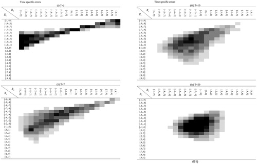
Figure B2. Joint distribution of first and second order serial correlations (R₁, R₂) when quadratic GCM with time-specific errors are correctly specified. Darker color indicates higher density.

Appendix B

References

- Ancona, D. G., Okhuysen, G. A., & Perlow, L. A. (2001). Taking time to integrate temporal research. Academy of Management Review, 26(4), 512–529.
- Alessandri, G., Caprara, G. V., & Tisak, J. (2012). A unified latent curve, latent state-trait analysis of the developmental trajectories and correlates of positive orientation. Multivariate Behavioral Research, 47(3), 341–368. doi: 10.1080/00273171.2012.673954
- Baayen, R. H., Davidson, D. J., & Bates, D. M. (2008). Mixed-effects modeling with crossed random effects for subjects and items. Journal of Memory and Language, 59(4), 390–412. doi: 10.1016/j.jml.2007.12.005
- Bates, D., Maechler, M., & Bolker, B. (2011). Lme4: Linear mixed-effects models using s4 classes (Version R package version 0.999375-39). Retrieved from http://CRAN.R-project.org/packagelme4
- Biesanz, J. C., Deeb-Sossa, N., Papadakis, A. A., Bollen, K. A., & Curran, P. J. (2004). The role of coding time in estimating and interpreting growth curve models. Psychological Methods, 9(1), 30–52. doi: 10.1037/1082-989x.9.1.30
- Bodenhausen, G. V. (1990). Stereotypes as judgmental heuristics: Evidence of circadian variations in discrimination. Psychological Science, 1(5), 319–322. doi: 10.1111/j.1467-9280.1990.tb00226.x
- Bolger, N., Davis, A., & Rafaeli, E. (2003). Diary methods: Capturing life as it is lived. Annual Review of Psychology, 54(1), 579–616. doi: 10.1146/annurev.psych.54.101601.145030
- Bollen, K. A., & Curran, P. J. (2004). Autoregressive latent trajectory (ALT) models: A synthesis of two traditions. Sociological Methods & Research, 32(3), 336–383. doi: 10.1177/0049124103260222
- Bollen, K. A., & Curran, P. J. (2006). Latent curve models: A structural equation perspective. Hoboken, NJ: John Wiley & Sons.
- Braun, M. T., Kuljanin, G., & DeShon, R. P. (2013). Spurious results in the analysis of longitudinal data in organizational research. Organizational Research Methods, 16(2), 302–330.
- Clark, H. H. (1973). The language-as-fixed-effect fallacy: A critique of language statistics in psychological research. Journal of Verbal Learning & Verbal Behavior, 12(4), 335–359. doi:10.1016/S0022-5371(73)80014-3
- Collins, L. M., & Sayer, A. G. (2001). New methods for the analysis of change. Washington, D.C.: American Psychological Association.
- Cudeck, R., & Harring, J. R. (2007). Analysis of nonlinear patterns of change with random coefficient models. Annual Review of Psychology, 58(1), 615–637.
- Curran, P. J., & Bollen, K. A. (2001). The best of both worlds: Combining autoregressive and latent curve models. In Collins, L. M. & Sayer, A. G. (Eds.), New methods for the analysis of change (pp.105–136). Washington, DC: American Psychological Association.
- de Ayala, R. J. (2009). The theory and practice of item response theory. New York: The Guilford Press.
- Duncan, T. E., Duncan, S. C., & Strycker, L. A. (2006). An introduction to latent variable growth curve modeling: Concepts, issues, and applications (2nd ed.). Mahwah, NJ: Lawrence Erlbaum Associates Publishers.
- Durbin, J., & Watson, G. S. (1950). Testing for serial correlation in least squares regression, I. Biometrika, 37(3–4), 409–428. doi: 10.1093/biomet/37.3-4.409.JSTOR2332391
- Durbin, J., & Watson, G. S. (1951). Testing for serial correlation in least squares regression, II. Biometrika, 38(1–2), 159–179. doi: 10.1093/biomet/38.1-2.159.JSTOR2332325
- Eccles, J. S., & Wigfield, A. (1995). In the mind of the achiever: The structure of adolescents' achievement task values and expectancy related beliefs. Personality and Social Psychology Bulletin, 21, 215–225. doi: 10.1177/0146167295213003
- Freeman, E., Heathcote, A., Chalmers, K., & Hockley, W. (2010). Item effects in recognition memory for words. Journal of Memory and Language, 62(1), 1–18. doi: 10.1016/j.jml.2009.09.004
- Fredricks, J. A., & Eccles, J. S. (2002). Children’s competence and value beliefs from childhood through adolescence: Growth trajectories in two male-sex-typed domains. Developmental Psychology, 38(4), 519–533. doi: 10.1037/0012-1649.38.4.519
- Frenzel, A. C., Goetz, T., Pekrun, R., & Watt, H. M. G. (2010). Development of mathematics interest in adolescence: Influences of gender, family, and school context. Journal of Research on Adolescence, 20, 507–537.
- Giraitis, L., Kapetanios, G., & Yates, T. (2014). Inference on stochastic time-varying coefficient models. Journal of Econometrics, 179(1), 46–65. doi: 10.1016/j.jeconom.2013.10.009
- Grimm, K. J., Ram, N., & Hamagami, F. (2011). Nonlinear growth curves in developmental research. Child Development, 82(5), 1357–1371. doi: 10.1111/j.1467-8624.2011.01630.x.
- Grimm, K. J., Steele, J. S., Ram, N., & Nesselroade, J. R. (2013). Exploratory latent growth models in the structural equation modeling framework. Structural Equation Modeling, 20(4), 568–591. doi:10.1080/10705511.2013.824775
- Hamaker, E. L., Ceulemans, E., Grasman, R. P. P. P., & Tuerlinckx, F. (2015). Modeling affect dynamics: State-of-the-art and future challenges. Emotion Review, 7(4), 316–322. doi: 10.1177/1754073915590619
- Hamaker, E. L., Kuiper, R. M., & Grasman, R. P. P. P. (2015). A critique of the cross-lagged panel model. Psychological Methods, 20(1), 102–116. doi:10.1037/a0038889
- Hedges, L. V., & Hedberg, E. (2007). Intraclass correlation values for planning group randomized trials in education. Educational Evaluation and Policy Analysis, 29(1), 60–87.
- Hertzog, C., & Nesselroade, J. R. (2003). Assessing psychological change in adulthood: An overview of methodological issues. Psychology and Aging, 18(4), 639–657. doi: 10.1037/0882-7974.18.4.639
- Judd, C. M., Westfall, J., & Kenny, D. A. (2012). Treating stimuli as a random factor in social psychology: A new and comprehensive solution to a pervasive but largely ignored problem. Journal of Personality and Social Psychology, 103(1), 54–69. doi: 10.1037/a0028347
- Judd, C. M., Westfall, J., & Kenny, D. A. (2017). Experiments with more than one random factor: Designs, analytic models, and statistical power. Annual Review of Psychology, 68(1), 601–625.
- Kenny, D. A., & Zautra, A. (2001). Trait-state models for longitudinal data. In L. M. Collins & A. G. Sayer (eds.), New methods for the analysis of change (pp. 243–263). Washington, DC: American Psychological Association.
- Kenward, M. G., & Roger, J. H. (1997). Small sample inference for fixed effects from restricted maximum likelihood. Biometrics, 53(3), 983–997. doi: 10.2307/2533558
- Kuznetsova, A., Brockhoff, P. B., & Christensen, R. H. B. (2015). lmerTest: Tests for random and fixed effects for linear mixed effect models (lmer objects of lme4 package). R package version 2.0-25. http://www.cran.r-project.org/package=lmerTest
- Kuznetsova, A., Brockhoff, P. B., & Christensen, R. H. B. (2017). lmerTest Package: Tests in linear mixed effects models. Journal of Statistical Software, 82(13), 1–26. doi: 10.18637/jss.v082.i13.
- Laird, N. M., & Ware, H. (1982). Random-effects models for longitudinal data. Biometrics, 38(4), 963–974.
- Lord, F.M., & Novick, M.R. (1968). Statistical theories of mental test scores. Menlo Park, CA: Addison-Wesley.
- Marsh, H. W., Pekrun, R., Parker, P. D., Murayama, K., Guo, J., Dicke, T., & Lichtenfeld, S. (2017). Long-term positive effects of repeating a year in school: Six-year longitudinal study of self-beliefs, anxiety, social relations, school grades, and test scores. Journal of Educational Psychology, 109(3), 425–438. doi: 10.1176/appi.ajp.2016.16020224
- May, C. P. (1999). Synchrony effects in cognition: The costs and a benefit. Psychonomic Bulletin & Review, 6(1), 142–147. doi: 10.3758/BF03210822
- McArdle, J. J. (1988). Dynamic but structural equation modeling of repeated measures data. In J. R. Nesselroade & R. B. Cattell (Eds.), The handbook of multivariate experimental psychology (pp. 561–614). New York, NY: Plenum Press.
- McArdle, J. J. (2009). Latent variable modeling of differences and changes with longitudinal data. Annual Review of Psychology, 60(1), 577–605. doi: 10.1146/annurev.psych.60.110707.163612.
- McArdle, J. J., Anderson, E., Birren, J. E., & Schaie, K. W. (1990). Latent variable growth models for research on aging: Handbook of the psychology of aging (3rd ed.). (pp. 21–44). San Diego, CA: Academic Press.
- McArdle, J. J., & Hamagami, F. (2001). Latent difference score structural models for linear dynamic analyses with incomplete longitudinal data. In L. M. Collins & A. G. Sayer (eds.), New methods for the analysis of change (pp. 139–175). Washington, DC: American Psychological Association.
- McArdle, J. J., & Nesselroade, J. R. (1994). Using multivariate data to structure developmental change. In S. H. Cohen & H. W. Reese (Eds.), Life-span developmental psychology: Methodological contributions. (pp. 223–267). New Jersey: Lawrence Erlbaum Associates.
- McArdle, J. J., & Nesselroade, J. R. (2014). Longitudinal data analysis using structural equation models. Washington, DC: American Psychological Association.
- Mehta, P. D., & Neale, M. C. (2005). People are variables too: Multilevel structural equation modeling. Psychological Methods, 10(3), 259–284. doi: 10.1037/1082-989X.10.3.259
- Meredith, W., & Horn, J. (2001). The role of factorial invariance in modeling growth and change. In L. M. Collins & A. G. Sayer (eds.), New methods for the analysis of change (pp. 203–240). Washington, DC: American Psychological Association.
- Meredith, W., & Tisak. J. (1984). Statistical considerations in Tuckerizing curves with emphasis on growth curves and cohort sequential analysis. Santa Barbara, CA: Paper presented at the annual meeting of the Psychometric Society.
- Meredith, W., & Tisak, J. (1990). Latent curve analysis. Psychometrika, 55(1), 107–122. doi: 10.1007/BF02294746
- Meyers, J. L., & Beretvas, S. N. (2006). The impact of inappropriate modeling of cross-classified data structures. Multivariate Behavioral Research, 41(4), 473–497. doi: 10.1207/s15327906mbr4104_3
- Murayama, K., Sakaki, M., Yan, V. X., & Smith, G. M. (2014). Type 1 error inflation in the traditional by-participant analysis to metamemory accuracy: A generalized mixed-effects model perspective. Journal of Experimental Psychology. Learning, Memory, and Cognition, 40(5), 1287–1306. doi:10.1037/a0036914
- Murray, D. M., & Blistein, J. L. (2003). Methods to reduce the impact of intraclass correlation in group-randomized trials. Evaluation Review, 27(1), 79–103.
- Potthoff, R. R., & Roy, S. N. (1964). A generalized multivariate analysis of variance model useful especially for growth curve problems. Biometrika, 51(3–4), 313–326. doi: 10.1093/biomet/51.3-4.313
- Preacher, K. J., & Hancock, G. R. (2015). Meaningful aspects of change as novel random coefficients: A general method for reparameterizing longitudinal models. Psychological Methods, 20(1), 84–101. doi: 10.1037/met0000028
- Primiceri, G. E. (2005). Time varying structural vector autoregressions and monetary policy. The Review of Economic Studies, 72(3), 821–852. doi: 10.1111/j.1467-937X.2005.00353.x
- Ram, N., & Grimm, K. J. (2015). Growth curve modeling and longitudinal factor analysis. In W. F. Overton & P. C. M. Molenaar (Eds.), Handbook of child psychology and developmental science: Theory & method (pp. 758–788). Hoboken, NJ: Wiley.
- Rao, C. R. (1965). The theory of least squares when the parameters are stochastic and its application to the analysis of growth curves. Biometrika, 52(3), 447–458.
- Rasbash, J., & Browne, W. J. (2001). Modeling non-hierarchical structures. In A. H. Leyland & H. Goldstein (Eds.), Multilevel modeling of health statistics (pp. 93–105). Chichester, UK: John Wiley and Sons.
- Raudenbush, S. W., & Bryk, A. (2002). Hierarchical linear models: Applications and data analysis methods (2nd ed.). Newbury Park, CA: Sage.
- Rentz, J. O., & Reynolds, F. D. (1981). Separating age, cohort and period effects in consumer behavior. Advances in Consumer Research, 8, 596–601.
- Satterthwaite, F. E. (1941). Synthesis of variance. Psychometrika, 6(5), 309–316.
- Schwarz, N., & Clore, G. L. (1983). Mood, misattribution, and judgements of well-being: Informative and directive functions of affective states. Journal of Personality and Social Psychology, 45(3), 513–523. doi:10.1037/0022-3514.45.3.513
- Schwarz, N. & Sudman, S. (Eds.) (1996). Answering questions: Methodology for determining cognitive and communicative processes in survey research. San Francisco, CA: Jossey-Bass Publications.
- Schaalje, G. B., McBride, J. B., & Fellingham, G. W. (2002). Adequacy of approximations to distributions of test statistics in complex mixed linear models using SAS Proc MIXED. Journal of Agricultural, Biological, and Environmental Statistics, 7(4), 512–524. doi: 10.1198/108571102726
- Shanken, J. (1990). Intertemporal asset pricing: An empirical investigation. Journal of Econometrics, 45(1–2), 99–120. doi: 10.1016/0304-4076(90)90095-B
- Shiyko, M. P., Lanza, S. T., Tan, X., Li, R., & Shiffman, S. (2012). Using the time-varying effect model (TVEM) to examine dynamic associations between negative affect and self confidence on smoking urges: Differences between successful quitters and relapsers. Prevention Science, 13(3), 288–299. doi: 10.1007/s11121-011-0264-z
- Singer, J. D. (1998). Using sas proc mixed to fit multilevel models, hierarchical models, and individual growth models. Journal of Educational and Behavioral Statistics, 23(4), 323–355. doi: 10.3102/10769986023004323
- Singer, J. D., & Willett, J. B. (2003). Applied longitudinal data analysis: Modeling change and event occurrence. Oxford, UK: Oxford University Press.
- Skrondal, A., & Rabe-Hesketh, S. (2004). Generalized latent variable modeling. Multilevel, longitudinal, and structural equation models. Boca Raton, FL: Chapman & Hall/CRC.
- Tanaka, A., & Murayama, K. (2014). Within-person analyses of situational interest and boredom: Interactions between task-specific perceptions and achievement goals. Journal of Educational Psychology, 106(4), 1122–1134.
- Usami, S. (2014). Generalized sample size determination formulas for experimental research with hierarchical data. Behavior Research Methods, 46(2), 346–356. doi: 10.3758/s13428-013-0387-1
- Walls, T. A. & Schafer, J. L. (Eds.) (2006). Models for intensive longitudinal data. New York, NY: Oxford University Press.
- Westfall, J., Kenny, D. A., & Judd, C. M. (2014). Statistical power and optimal design in experiments in which samples of participants respond to samples of stimuli. Journal of Experimental Psychology: General, 143, 2020–2045.
- Wigfield, A., & Eccles, J. S. (2000). Expectancy-value theory of motivation. Contemporary Educational Psychology, 25, 68–81. doi: 10.1006/ceps.1999.1015
- Wu, W., West, S. G., & Taylor, A. B. (2009). Evaluating model fit for growth curve models: Integration of fit indices from SEM and MLM frameworks. Psychological Methods, 14, 183–201.