Integrating covariates into circumplex structures: an extension procedure for Browne’s circular stochastic process model

Abstract

Circumplex structures are elements of various psychological domains. Most work focuses on assessing the circular ordering of circumplex indicators and their relationships with covariates. In this article, an extension procedure for Browne’s circumplex model is presented. Our approach models the relationships among circumplex indicators and the relationships of covariates with a latent circumplex simultaneously without affecting the circumplex indicators’ positions on the circumplex. The approach builds upon Browne’s Fourier series parameterization of a correlation function, which is used to model the latent circumplex correlation structure. It extends the shape of the correlation function to the profile of each covariate’s correlations with the circumplex. The model is specified in the framework of structural equation modeling, thereby making it possible to test various hypotheses. Procedures are presented for deriving interval estimates for the parameters that relate the covariates to the circumplex. The model is compared to other approaches for assessing the relationships of a circumplex with covariates. The results of the exemplary applications and a simulation study were in favor of the suggested model. The approach is furthermore illustrated with a real-data example, focusing on the relationships between the interpersonal circumplex and the rivalry and admiration aspects of narcissism.

Keywords:

• circumplex structures
• factor extension
• structural equation modeling
• Fourier series
• interpersonal circumplex

Circumplex structures are key elements of a variety of psychological domains, such as interpersonal behavior (Leary, 1957), personality traits (Hofstee, de Raad, & Goldberg, 1992), vocational interests (Tracey & Rounds, 1993), emotions (Watson, Wiese, Vaidya, & Tellegen, 1999), color perception (Shepard, 1978), psychopathology (Gurtman, 1994), and values (Schwartz, 1992). A circumplex postulates a specific structure of similarities among content types that belong to one construct domain (e.g., types of interpersonal behavior). According to the circumplex, the variables’ intercorrelations can be represented as a mathematical function of their positions on the circumference of a circle (Guttman, 1954). Recent approaches for analyzing circumplex structures are variants of latent variable models that acknowledge that the correlation patterns between fallible observed scores could deviate from the circumplex correlation structures located at the latent level. To overcome the necessity of choosing a specific function, Browne (1992) developed a flexible model based on a Fourier series approximation of an arbitrary function suitable for the circumplex. Browne’s (1992) Circular Stochastic Process Model for the Circumplex (SPMC) has gained widespread popularity (e.g., DeGeest & Schmidt, 2015; Šverko, Babarović, & Međugorac, 2014).

Various psychological disciplines have agreed upon the validity of the circumplex for various constructs, and research is moving on towards relating covariates to an existing circumplex. Examples include the relationships between the interpersonal circumplex and the Big Five personality variables (DeYoung, Weisberg, Quilty, & Peterson, 2013), and relationships between the vocational interest circumplex and abilities (Armstrong, Day, McVay, & Rounds, 2008), among others. To this end, most research has employed the structural summary method (SSM; Gurtman, 1994). In the SSM, the vector of observed correlations of the circumplex indicators with a covariate is modeled by a cosine function. However, despite its elegant appeal, the SSM can be optimized in multiple ways to make it compatible with the more sophisticated latent SPMC. The SSM is limited because (1) the cosine function is less flexible than the Fourier series, (2) the SSM requires the locations of the indicators of the circumplex to be known, (3) the method disregards the fallible nature of circumplex indicators, and (4) in its standard setup, the SSM does not provide interval estimates for the projection of a covariate onto a circumplex (cf. Zimmermann & Wright, 2017).

As an alternative to the SSM, Yik and Russel (2004) proposed the CIRCUM-extension, which is based on the SPMC. Their model builds upon the assumption that covariates can be treated as indicators of the circumplex. This assumption limits the generality of the procedure because covariates might not have the same properties as the indicators of the circumplex, although they might be related to a circumplex. In addition, similar to the SSM, the procedure is not intended to provide interval estimates for its key parameters.

The aim of this article is to provide a flexible approach that makes it possible to relate covariates to a circumplex as represented by the SPMC while overcoming the limitations of the CIRCUM-extension and the SSM. In the proposed model, the circumplex indicators’ and the covariates’ locations on the circumplex are estimated simultaneously, while ensuring that the circumplex indicators’ locations are not affected by the inclusion of covariates. Our model provides point and interval estimates of the covariates’ locations on a circumplex. The model is specified in the structural equation modeling (SEM) framework, thereby allowing a variety of hypotheses to be tested.

In the next section, we introduce the SPMC, the SSM, the CIRCUM-extension, and the ideas behind the new model. To this end, we give examples based on data reported by Gurtman (1992b). We then present the new approach. In this section, we show how the SPMC can be specified as a confirmatory factor analysis (CFA), how covariates can be included in the model, and how the precision of the estimates of the parameters that relate covariates to the latent circumplex can be assessed. Finally, we examine the new model by means of a simulation study, and apply it to a new dataset, thereby demonstrating its utility for applied research.

Models for circumplex structures and their relationships with covariates

We introduce the circumplex by recurring on the interpersonal circumplex model (IPC; Wiggins, 2003). In the IPC, it is assumed that types of interpersonal behavior are organized such that their similarities can be represented by their positions on the perimeter of a circle, with similarity between types of behavior determining their relative position and proximity. Instruments developed in the context of the IPC measure eight types of interpersonal behavior (represented by the synthetic codes: LM, NO, PA, BC, DE, FG, HI, and JK). The theoretical locations of the types of interpersonal behavior on the IPC are shown in Figure 1.

Figure 1. Graphical representation of an equally spaced perfect circumplex (left panel), and the corresponding circulant correlation matrix (right panel). Examples drawn from the Interpersonal Circumplex Model as assessed by the Interpersonal Adjective Scales. LM = Warm-Agreeable, NO = Gregarious-Extraverted, PA = Assured-Dominant, BC = Arrogant-Calculating, DE = Coldhearted, FG = Aloof-Introverted, HI = Unassured-Submissive, JK = Unassuming-Ingenuous.

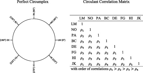
The strong version of the IPC assumes that all variables are equidistantly distributed on the circle, also known as a perfect circumplex (Guttman, 1954). In that case, only four levels of proximity exist, which means that the correlation matrix of the indicators’ true scores is structured as shown in the second panel of Figure 1 (a circulant matrix). However, even if the circumplex hypothesis holds true, deviations of correlations among manifest indicators from a circulant matrix are likely to occur for two reasons. First, psychological measures are fallible, which means that their correlations are likely to deviate from the relationships of the underlying true scores. Second, true scores need not be equidistantly distributed on the circle; a structure called a quasi-circumplex (Guttman, 1954). The SPMC (Browne, 1992) is a model that makes it possible to test whether the correlation pattern among indicator variables can be explained by a latent perfect or quasi-circumplex (for an overview of alternative methods, see Tracey, 2000). An empirically derived quasi-circumplex structure should, of course, be judged not only on the basis of the model-data fit; the results should also be evaluated in light of theory. Researchers should at least examine whether the empirically derived order of variables agrees with the order predicted by the theory (e.g., Nagy, Trautwein, & Lüdtke, 2010), and they could, in addition, quantify the congruence between the empirical results and the theoretical model (e.g., Fisher, Heise, Bohrnstedt, & Lucke, 1985).

In research areas where evidence for the validity of circumplex structures has been accumulated, the question emerges of whether covariates are meaningfully related to a circumplex (e.g., Gurtman & Balakrishnan, 1998). Traditional methods, such as the SSM, examine whether the correlations of circumplex indicators with covariates are in line with the circumplex structure (Gurtman, 1992a). However, when the circumplex is regarded as a latent entity, covariates should be related to the true scores of the circumplex indicators. Ideally, the shape of the correlational profile of a covariate with the true scores should agree with the shape of the profiles of correlations among the true scores of the circumplex indicators.

In the following subsection, we first introduce the SPMC (Browne, 1992). We then explain the SSM (Gurtman, 1994) and the CIRCUM-extension (Yik & Russel, 2004) that allow covariates to be related to a circumplex. We discuss the strengths and weaknesses of the SSM and CIRCUM-extension, and introduce the basic ideas of our new extension procedure for the SPMC. In order to exemplify the approaches introduced, we report a first empirical application based on data reported by Gurtman (1992b). Details on the specification of the SPMC and our extension procedure are provided in the next major section.

The circular stochastic process model for the circumplex

In Browne’s (1992) SPMC, each circumplex indicator, $x_j$ (j = 1, 2, …, J), is assumed to be made up of a common (or true) score, $c_j$, and a unique part, $u_j$ (details are given in a later part of this article). The correlation between two indicators $x_j$ and $x_k$, ${\rho }_{x_{j,}{x}_k}$, is related to the common scores’ correlation, ${\rho }_{c_{j,}{c}_k}$, as: (1) $${\rho }_{x_{j,}{x}_k}=h_j{\rho }_{c_{j,}{c}_k}{h}_k,$$(1) where $h_j$ and $h_k$ stand for the communalities of the indicators $x_j$ and $x_k$.

The structure of correlations among common scores is the key aspect of the circumplex. In a circumplex, the size of ${\rho }_{c_{j,}{c}_k}$ is related to the distance between the locations of $c_j$ and $c_k$ on the perimeter of a circumplex (Browne, 1992): (1) When $c_j$ and $c_k$ occupy the same position, their correlation is one, (2) the correlation between $c_j$ and $c_k$ decreases as a sole function of the length of the closest connecting path and is not related to the direction of the path, and (3) ${\rho }_{c_{j,}{c}_k}$ achieves its minimum when $c_j$ and $c_k$ occupy opposite positions on the circumplex. In order to specify a correlation structure of common scores that fulfills these requirements, Browne (1992) proposed expressing these correlations by a suitable correlation function that is approximated by a Fourier series: (2) $${\rho }_{c_j,c_k}={\beta }_0^2+\sum _{m=1}^M{\beta }_m^2\text{cos}\left[\begin{array}{c}m\left({\theta }_j-{\theta }_k\right)\end{array}\right],$$(2) where the $\theta$-parameters stand for the common scores’ angular locations. The $\beta$-parameters are constrained to be positive and the sum of their squares is constrained to be one (${\beta }_0^2+{\sum }_{m=1}^M{\beta }_m^2=1$). When M is set to one (M = 1), Equation 2(2) $${\rho }_{c_j,c_k}={\beta }_0^2+\sum _{m=1}^M{\beta }_m^2\text{cos}\left[\begin{array}{c}m\left({\theta }_j-{\theta }_k\right)\end{array}\right],$$(2) reduces to a cosine function. In this case, the SPMC can be conceived as the confirmatory counterpart of the three-dimensional exploratory factor model often applied in practice (Nagy, Marsh, Lüdtke, & Trautwein, 2009; Tracey, 2000).¹ By setting the number of components M to be sufficiently high, any correlation function suitable for the circumplex can be approximated, which means that the Fourier series can, by itself, be regarded as a correlation function (Browne, 1992, p. 485).

Equation 2(2) $${\rho }_{c_j,c_k}={\beta }_0^2+\sum _{m=1}^M{\beta }_m^2\text{cos}\left[\begin{array}{c}m\left({\theta }_j-{\theta }_k\right)\end{array}\right],$$(2) provides a maximum correlation of one when the angular locations of both variables correspond to each other (i.e., ${\theta }_j-{\theta }_k$ = 0), and achieves its minimum when the angular locations of $c_j$ and $c_k$ are separated by 180° ($\pi$ = 3.14159… in radian units, i.e., $\left|{\theta }_j-{\theta }_k\right|=\pi$). However, the Fourier correlation function does not generally guarantee monotonic decreasing correlations over the interval $0\le {|\theta }_k-{\theta }_j|\le \pi$. Browne (1992, p. 486) therefore advised users to apply a fairly small number of components M (i.e., M < J/2).

In Equation 2(2) $${\rho }_{c_j,c_k}={\beta }_0^2+\sum _{m=1}^M{\beta }_m^2\text{cos}\left[\begin{array}{c}m\left({\theta }_j-{\theta }_k\right)\end{array}\right],$$(2) , ${\beta }_0^2$ reflects the level component of the correlation function over the interval 0 to $2\pi$ (i.e., the average correlation defined over each possible angular position). The sum ${\sum }_{m=1}^M{\beta }_m^2=1-{\beta }_0^2$ gives the maximum positive deviation from the level that occurs at ${\theta }_j={\theta }_k$. The minimum correlation given at a separation of $\pi$ (i.e., 180°) deviates by $\left({\beta }_2^2+{\beta }_4^2+{\beta }_6^2+\dots \right)-\left({\beta }_1^2+{\beta }_3^2+{\beta }_5^2+\dots \right)$ from ${\beta }_0^2$. 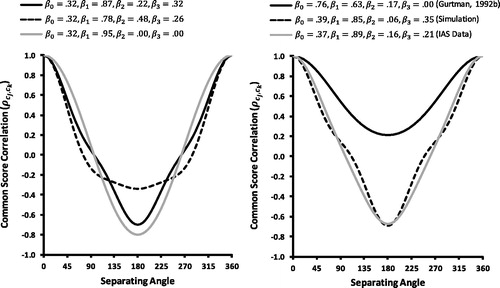The relative size of the ${\beta }_m$-parameters (for m > 0) controls the shape of the correlation function. Figure 2 provides some examples based on a Fourier series with M = 3 components. It also includes a cosine function (i.e., ${\beta }_2={\beta }_3=0$) as a comparison. The SPMC is quite flexible in approximating different shapes of correlation functions, even with a fairly small number of components M.

Figure 2. Left panel: Examples of SPMC correlation functions with different configurations of $\beta$-parameters and M = 3 components in the Fourier series. The correlation function with ${\beta }_2={\beta }_3=0$ corresponds to the cosine function. Right panel: SPMC correlation functions estimated on the basis of the IIP-C (Gurtman,1992b), specified in the simulation study (Simulation), and estimated on the basis of the IAS (IAS Data).

As shown in Figure 2, the average correlation between all possible levels of separating angles is solely determined by ${\beta }_0$, and the term $1-{\beta }_0^2$ determines the scatter of the correlation function. Therefore, $1-{\beta }_0^2$ can be interpreted as the content sensitivity of the circumplex: When ${\beta }_0$ takes a value of zero, correlations between common scores are solely determined by the similarity of their contents. When ${\beta }_0$ equals one, all common scores are perfectly correlated, which means that the correlation structure is not content sensitive.

The structural summary method

The SSM is used to relate a covariate $y_q$ to a circumplex. It uses a cosine function to model the correlations of the circumplex indicators with $y_q$: (3) $${\rho }_{x_{j,}{y}_q}=g_{0,q}+g_{1,q}\text{cos}\left({\theta }_j-d_q\right),$$(3) where $g_{0,q}$, $g_{1,q}$, and $d_q$ are the coefficients that are estimated by the SSM. $g_{0,q}$ represents the average correlation of $y_q$ with the J circumplex indicators, $g_{1,q}$ is the amplitude of the correlation function that is interpreted as the content sensitivity of $y_q$, and $d_q$ refers to the angular location on the circumplex for which the maximum correlation with $y_q$ is expected. ${\theta }_j$ refers to the angular location of the circumplex indicator $x_j$ that is assumed to be known prior to the analysis. In applications of the SSM, the values of $\theta$ are typically fixed according to a perfect circumplex (Gurtman & Pincus, 2003). The parameters of the SSM are estimated in a least squares manner by minimizing the sum of squared discrepancies between estimated correlations ${\rho }_{x_{j,}{y}_q}$ and sample correlations $r_{x_{j,}{y}_q}$.²

The coefficients $g_{1,q}$ and $d_q$ can be used to locate the covariate $y_q$ on the circumplex (e.g., Miller, Price, Gentile, Lynam, & Campbell, 2012). The location of $y_q$ is described by a vector drawn from the origin of the circumplex, with lengths equal to $g_{1,q}$ and an orientation equal to $d_q$, which means that the endpoint of the vector has coordinate values of $g_{1,q}\text{cos}\left(d_q\right)$ on the x-axis, and $g_{1,q}\text{sin}\left(d_q\right)$ on the y-axis.

The CIRCUM-extension

The CIRCUM-extension (Yik & Russel, 2004) addresses the issues of fallible indicators and of circumplex correlation functions other than the cosine function. The model is a two-step procedure, in which the parameters of the SPMC are first estimated without considering the covariates. These parameters are then fixed to their estimated values and the SPMC is applied to the full set of variables that includes covariates. In the second step, only the parameters pertaining to the covariates are estimated.

In the CIRCUM-extension, covariates are treated as circumplex indicators, which means that for each covariate $y_q$ two parameters are estimated: An angular location, ${\delta }_q$, and a communality index, $h_q$ (Equations 1(1) $${\rho }_{x_{j,}{x}_k}=h_j{\rho }_{c_{j,}{c}_k}{h}_k,$$(1) and 2(2) $${\rho }_{c_j,c_k}={\beta }_0^2+\sum _{m=1}^M{\beta }_m^2\text{cos}\left[\begin{array}{c}m\left({\theta }_j-{\theta }_k\right)\end{array}\right],$$(2) ). As the $\beta$- and $\theta$-parameters of the SPMC are fixed to their initial estimates, the covariates’ common parts are embedded in the same correlation function that applies to the circumplex indicators’ common scores. The model implies the following relationships of a covariate $y_q$ with the indicators’ common scores: (4) $${\rho }_{c_j,y_q}=h_q\left\{{\widehat{\beta }}_0^2+\sum _{m=1}^M{\widehat{\beta }}_m^2\text{cos}\left[\begin{array}{c}m\left({\widehat{\theta }}_j-{\delta }_q\right)\end{array}\right]\right\}.$$(4) where the parameters that are marked by a hat are fixed to their initial estimates.

Equation 4(4) $${\rho }_{c_j,y_q}=h_q\left\{{\widehat{\beta }}_0^2+\sum _{m=1}^M{\widehat{\beta }}_m^2\text{cos}\left[\begin{array}{c}m\left({\widehat{\theta }}_j-{\delta }_q\right)\end{array}\right]\right\}.$$(4) shows that, in the CIRCUM-extension, $h_q$ transforms the level and the scatter of the common scores’ correlation function into $y_q$’s average correlation with the indicators’ common scores, $h_q{\beta }_0^2$, and its content sensitivity, $h_q\left(1-{\beta }_0^2\right)$. Therefore, $h_q$ provides the covariate’s $y_q$ content sensitivity relative to the content sensitivity of the circumplex. As a consequence, a vector with an endpoint with x- and y-coordinates $h_q\text{cos}\left({\delta }_q\right)$, and $h_q\text{sin}\left({\delta }_q\right)$, respectively, can be used to locate $y_q$ on a circle with a unit radius.

Towards a new extension procedure for the SPMC

The use of a single parameter, $h_q$, in Equation 4(4) $${\rho }_{c_j,y_q}=h_q\left\{{\widehat{\beta }}_0^2+\sum _{m=1}^M{\widehat{\beta }}_m^2\text{cos}\left[\begin{array}{c}m\left({\widehat{\theta }}_j-{\delta }_q\right)\end{array}\right]\right\}.$$(4) , which relates a covariate to the level and scatter of the correlation function of the common scores, is quite restrictive. In real applications, it might turn out that a covariate is content sensitive, although it is not sensitive to the level component of the circumplex (and vice versa). A possible way of overcoming this restriction is to modify Equation 4(4) $${\rho }_{c_j,y_q}=h_q\left\{{\widehat{\beta }}_0^2+\sum _{m=1}^M{\widehat{\beta }}_m^2\text{cos}\left[\begin{array}{c}m\left({\widehat{\theta }}_j-{\delta }_q\right)\end{array}\right]\right\}.$$(4) by replacing $h_q$ with two parameters, such that: (5) $${\rho }_{c_j,y_q}={\gamma }_{0,q}{\widehat{\beta }}_0^2+{\gamma }_{1,q}\sum _{m=1}^M{\widehat{\beta }}_m^2\text{cos}\left[\begin{array}{c}m\left({\widehat{\theta }}_j-{\delta }_q\right)\end{array}\right].$$(5)

The parameter ${\gamma }_{0,q}$ measures the average correlation of $y_q$ with the common scores $c_j$ relative to the level of their correlation function, and ${\gamma }_{1,q}$ quantifies the content sensitivity of $y_q$ with respect to the latent circumplex relative to its content sensitivity. Similar to the SSM and the CIRCUM-extension, ${\delta }_q$ provides the angle on the latent circumplex at which the maximum correlation of a covariate with an indicator’s common score is predicted to occur. Equation 5(5) $${\rho }_{c_j,y_q}={\gamma }_{0,q}{\widehat{\beta }}_0^2+{\gamma }_{1,q}\sum _{m=1}^M{\widehat{\beta }}_m^2\text{cos}\left[\begin{array}{c}m\left({\widehat{\theta }}_j-{\delta }_q\right)\end{array}\right].$$(5) allows a covariate $y_q$ to be located on a circumplex by means of a vector drawn from the origin of a unit circle with an endpoint with x- and y-coordinates of ${\gamma }_{1,q}\text{cos}\left({\delta }_q\right)$, and ${\gamma }_{1,q}\text{sin}\left({\delta }_q\right)$, respectively.

Equation 5(5) $${\rho }_{c_j,y_q}={\gamma }_{0,q}{\widehat{\beta }}_0^2+{\gamma }_{1,q}\sum _{m=1}^M{\widehat{\beta }}_m^2\text{cos}\left[\begin{array}{c}m\left({\widehat{\theta }}_j-{\delta }_q\right)\end{array}\right].$$(5) combines features of the SSM and CIRCUM-extension. Similar to the SSM, it does not require a covariate to have the same sensitivity for the level and the scatter of the circumplex correlation function. Similar to the CIRCUM-extension, it describes a covariate’s relationship with a latent circumplex, and ensures that the covariate’s pattern of correlations has the same shape as the circumplex correlation function (Equation 2(2) $${\rho }_{c_j,c_k}={\beta }_0^2+\sum _{m=1}^M{\beta }_m^2\text{cos}\left[\begin{array}{c}m\left({\theta }_j-{\theta }_k\right)\end{array}\right],$$(2) ). However, in Equation 5(5) $${\rho }_{c_j,y_q}={\gamma }_{0,q}{\widehat{\beta }}_0^2+{\gamma }_{1,q}\sum _{m=1}^M{\widehat{\beta }}_m^2\text{cos}\left[\begin{array}{c}m\left({\widehat{\theta }}_j-{\delta }_q\right)\end{array}\right].$$(5) , the $\beta$- and $\theta$-parameters are treated as known although they are estimated on the basis of the same sample. As a solution to that problem, we propose an SEM specification that allows all parameters to be estimated simultaneously and sound interval estimates to be computed for the $\gamma$- and $\delta$-parameters.

A first empirical illustration of the procedures introduced

In order to provide an example of the procedures introduced so far, we report the key results derived by applying the methods to an existing dataset. Table 1 presents the correlations among the subscales of the Inventory of Interpersonal Problems Circumplex (IIP-C; Alden, Wiggins, & Pincus, 1990) and their relationships with a measure of sociability (reverse coded) in a sample of N = 163 undergraduates, reported by Gurtman (1992b). We report only the most important results, thereby highlighting the differences between the SSM, the CIRCUM-extension, and the preliminary new extension procedure for the SPMC. A more detailed example of the new model, which is based on a larger sample, will be presented in a later section.

Table 1. Descriptive statistics for the IIP-C and sociability scales reported by Gurtman (1992b) (correlations in the upper triangular matrix) and the IAS and NARQ Scales assessed in this investigation (correlations in the lower triangular matrix).

	Correlations									Gurtman (1992b)		Our Data
	LM	NO	PA	BC	DE	FG	HI	JK	$y_1$	SD	Alpha	SD	Alpha
LM		.470	.321	.220	.279	.359	.460	.712	−.014	0.62	.730	0.880	.820
NO	.565		.682	.459	.199	.181	.207	.339	−.091	0.59	.722	0.945	.817
PA	.072	.589		.711	.455	.415	.184	.159	.088	0.67	.775	1.142	.868
BC	−.356	.037	.478		.654	.580	.280	.135	.218	0.90	.875	1.127	.792
DE	−.513	−.293	.080	.640		.728	.460	.187	.360	0.74	.779	1.038	.850
FG	−.306	−.615	−.344	.244	.560		.630	.362	.485	0.78	.792	1.241	.860
HI	.039	−.491	−.658	−.189	.172	.603		.643	.263	0.75	.768	1.194	.841
JK	.388	−.063	−.363	−.327	−.126	.219	.603		.012	0.72	.749	0.936	.730
$y_1$	.065	.363	.536	.317	.155	−.144	−.345	−.188		4.16	.787	0.828	.833
$y_2$	−.338	−.244	.087	.551	.608	.396	.140	−.102	.333			0.812	.835

Notes. Data reported by Gurtman (1992b): LM = Overly Nurturant, NO = Intrusive, PA = Domineering, BC = Vindictive, DE = Cold, FG = Socially Avoidant, HI = Nonassertive, JK = Exploitable, ${\mathrm{y}}_1$ = Sociability (reverse coded); Our data: LM = Warm-Agreeable, NO = Gregarious-Extraverted, PA = Assured-Dominant, BC = Arrogant-Calculating, DE = Coldhearted, FG = Aloof-Introverted, HI = Unassured-Submissive, JK = Unassuming-Ingenuous, $y_1$ = Admiration, $y_2$ = Rivalry.

In the first step, the SPMC was applied to the IIP-C. A model with M = 2 components in the Fourier series provided a good representation of the data. The correlation function estimated by the SPMC (second panel of Figure 2) had a stronger level component (${\widehat{\beta }}_0^2$ = .58), and a lower content sensitivity ($1-{\widehat{\beta }}_0^2$ = .42) than the examples given in the first panel of Figure 2. The SPMC indicated that the IIP-C had a quasi-circumplex structure (Figure 3). The indicators’ communalities ranged from ${\widehat{h}}_{LM}$ = .80 to ${\widehat{h}}_{FG}$ = .91.

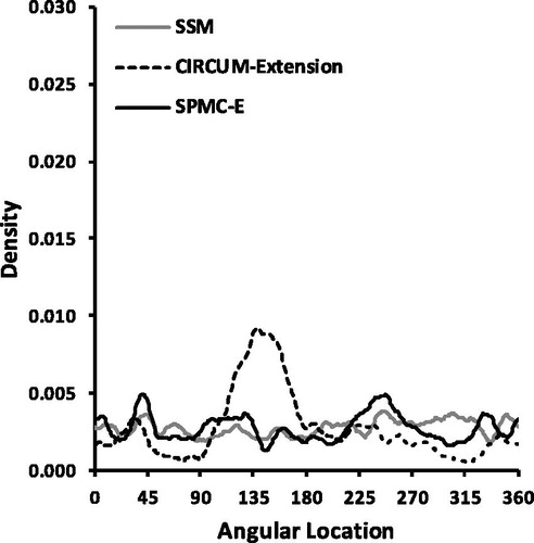
Figure 3. Results of the SSM, CIRCUM-extension, and the preliminary extension of the SPMC used for placing the sociability scale (reverse coded) onto the Interpersonal Circumplex as assessed by the IIP-C. Left panels: Sample correlations (SSM) or rescaled covariances (CIRCUM-extension and SPMC extension) and model-implied correlations. Right panels: Vector representations of relationships. LM = Overly Nurturant, NO = Intrusive, PA = Domineering, BC = Vindictive, DE = Cold, FG = Socially Avoidant, HI = Nonassertive, JK = Exploitable

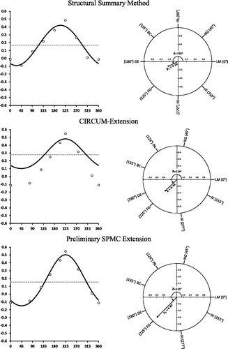
In the next step, we subjected the correlations of sociability with the IIP-C scales to the SSM, where the $\theta$-parameters were fixed according to Figure 1. The SSM yielded an average correlation of ${\widehat{g}}_{0,q}$ = .17, a content sensitivity of ${\widehat{g}}_{1,q}$ =.26, and an angular location of ${\widehat{d}}_q$ = 205.2°. Figure 3 show that the observed and fitted correlations had a high correspondence. The projection of sociability onto the circumplex (Figure 3) showed that this variable was located between the DE (cold; 180°) and FG scales (socially avoidant; 225°).

The CIRCUM-extension estimated the communality of sociability as ${\widehat{h}}_q$ = .48, and its angular location as ${\widehat{\delta }}_q$ = 224.4°; a location near to FG (socially avoidant; 224.9°), given by the SPMC. In order to make the estimate of the covariate’s content sensitivity comparable to the estimate provided by the SSM, we calculated the absolute content sensitivity implied by the CIRCUM-extension: ${\widehat{h}}_q\left(1-{\widehat{\beta }}_0^2\right)$ = .20. Compared to the SSM, the CIRCUM-extension indicated sociability to have a lower content sensitivity. Figure 3 depicts the model-implied profile of correlations, ${\rho }_{c_j,y_q}$, as well as the covariances of the circumplex indicators that were rescaled to the metric of their common scores (variables $x_j^{*}$, which are introduced in a later part of the article) with the standardized covariate. Optimally, these covariances show a close correspondence to the estimates of ${\rho }_{c_j,y_q},$ but this was not the case in this analysis.

The application of the extension to the SPCM given in Equation 5(5) $${\rho }_{c_j,y_q}={\gamma }_{0,q}{\widehat{\beta }}_0^2+{\gamma }_{1,q}\sum _{m=1}^M{\widehat{\beta }}_m^2\text{cos}\left[\begin{array}{c}m\left({\widehat{\theta }}_j-{\delta }_q\right)\end{array}\right].$$(5) gave the following estimates: ${\widehat{\gamma }}_{0,q}$ = .27, ${\widehat{\gamma }}_{1,q}$ = .83, and ${\widehat{\delta }}_q$ = 225.3°. These results indicate that sociability had a stronger content sensitivity than that suggested by the CIRCUM-extension and the SSM [i.e., ${\widehat{\gamma }}_{1,q}\left(1-{\widehat{\beta }}_0^2\right)$ = .35]. In addition, the model provided a good correspondence of the predicted correlations to the rescaled covariances.

The results reported in this section highlight some issues that are of relevance in applied settings. First, the results of the SPMC indicated that circumplex indicators were better aligned to a quasi-circumplex; a typical result in applied research (e.g., Gurtman & Pincus, 2000). Therefore, the assumption of a perfect circumplex that is typically imposed on the SSM is likely to affect the results. Second, circumplex indicators typically have nonzero unique components. Hence, analyses conducted on the basis of observed variables are likely to underestimate a covariate’s content sensitivity. Third, covariates might not have the same sensitivity for the level and scatter components of the circumplex. Erroneously including this assumption could therefore affect the conclusions about a covariate’s content sensitivity.

An extension procedure for the circular stochastic process model for the circumplex

Our procedure is specified in the framework of SEM, and is applied to a sample covariance matrix ${\mathit{S}}_{\left(\mathit{x},\mathit{y}\right),(\mathit{x},\mathit{y})}$ that extends the covariance matrix of circumplex indicators, ${\mathit{S}}_{\mathit{x},\mathit{x}}$, by Q covariates $y_q$ (q = 1, 2, …, Q). ${\mathit{S}}_{\left(\mathit{x},\mathit{y}\right),(\mathit{x},\mathit{y})}$ is structured as: (6) $${\mathit{S}}_{\left(\mathit{x},\mathit{y}\right),(\mathit{x},\mathit{y})}=\left[\begin{array}{cc}{\mathit{S}}_{\mathit{x},\mathit{x}}& {\mathit{S}}_{\mathit{x},\mathit{y}}\\ {\mathit{S}}_{\mathit{y},\mathit{x}}& {\mathit{S}}_{\mathit{y},\mathit{y}}\end{array}\right] ,$$(6) where ${\mathit{S}}_{\mathit{y},\mathit{y}}$ is the covariance matrix of covariates, and ${\mathit{S}}_{\mathit{y},\mathit{x}}$ encompasses the covariances of the circumplex indicators with the covariates. In our approach, the SPMC is used to approximate ${\mathit{S}}_{\mathit{x},\mathit{x}}$ by its model-implied covariance matrix ${\mathit{\Sigma }}_{\mathit{x},\mathit{x}}$, whereas ${\mathit{S}}_{\mathit{y},\mathit{y}}$ and ${\mathit{S}}_{\mathit{y},\mathit{x}}$ are approximated by the extension part of the model by ${\mathit{\Sigma }}_{\mathit{y},\mathit{y}}$ and ${\mathit{\Sigma }}_{\mathit{y},\mathit{x}}$, such that: (7) $${\mathbf{\Sigma }}_{\left(\mathit{x},\mathit{y}\right),(\mathit{x},\mathit{y})}=\left[\begin{array}{cc}{\mathbf{\Sigma }}_{\mathit{x},\mathit{x}}& {\mathbf{\Sigma }}_{\mathit{x},\mathit{y}}\\ {\mathbf{\Sigma }}_{\mathit{y},\mathit{x}}& {\mathbf{\Sigma }}_{\mathit{y},\mathit{y}}\end{array}\right].$$(7)

We first show how to specify the SPMC as a CFA, which means that we first consider the model for ${\mathit{\Sigma }}_{\mathit{x},\mathit{x}}$. We then extend the SPMC so that it provides a model for ${\mathbf{\Sigma }}_{\left(\mathit{x},\mathit{y}\right),(\mathit{x},\mathit{y})}$.

CFA parameterization of Browne’s SPMC

To estimate the SPMC, Browne provided the CIRCUM program (Browne, 1995). More recently, routines have been developed that allow the model to be estimated by other software packages, such as R (Grassi, Luccio, & Di Blas, 2010) and SAS (Yung, Browne, & Zhang, 2015). As we will show, the SPMC can also be specified as a CFA, thereby allowing its estimation by any SEM software that makes it possible to incorporate nonlinear parameter constraints. These requirements are fulfilled in the LISREL (Jöreskog & Sörbom, 1993), Mplus (Muthén & Muthén, 1998–2010), and Mx (Neale et al., 2016) programs. We describe the model in its general version by recurring on variables given in their raw metric. In order to simplify the specification, we provide a slightly different, but statistically equivalent parameterization of the SPMC than Browne (1992).

In the CFA parametrization, the J × 1 vector of circumplex indicators for person i (i = 1, 2, …, N) ${\mathit{x}}_{\mathit{i}}$ is expressed as a function of the J × 1 vector of rescaled variables ${\mathit{x}}_{\mathit{i}}^{\mathit{*}}$: (8) $${\mathit{x}}_{\mathit{i}}={\mathit{\mu }}_{\mathit{x}}+{\mathit{\zeta }}_{\mathit{x},\mathit{x}}{\mathit{x}}_{\mathit{i}}^{\mathit{*}},$$(8) where ${\mathit{\mu }}_{\mathit{x}}$ is a J × 1 vector of means, and ${\mathit{\zeta }}_{\mathit{x},\mathit{x}}$ is a J × J diagonal matrix of scaling constants. The rescaled scores are assumed to be composed of a common and a unique part: (9) $${\mathit{x}}_{\mathit{i}}^{\mathit{*}}={\mathit{c}}_{\mathit{i}}+{\mathit{\nu }}_{{\mathit{x}}^{\mathit{*}}{\mathit{x}}^{\mathit{*}}}{\mathit{u}}_{\mathit{i}},$$(9) where ${\mathit{c}}_{\mathit{i}}$ stands for the person i’s J × 1 vector of common scores, ${\mathit{u}}_{\mathit{i}}$ for i’s J × 1 vector of unique factor scores, and ${\mathit{\nu }}_{{\mathit{x}}^{\mathit{*},}{\mathit{x}}^{\mathit{*}}}$ is a J × J diagonal matrix of unique factor loadings. The common and the unique parts are both specified to have unit variances and zero means. Unique factors are assumed to be uncorrelated with each other, as well as with any other common score. Hence, the covariance matrix of unique factors is a J × J identity matrix, and the covariance matrix of common scores corresponds to a J × J correlation matrix ${\mathit{\rho }}_{\mathit{c},\mathit{c}}$.

In the SPMC, the J common scores are not represented as separate variables because they are specified as being fully determined by a smaller set of common factors, so that the unique factors are identified. To this end, 1 + 2 M mutually orthogonal common factors with unit variance are introduced, such that ${\mathit{\rho }}_{\mathit{c},\mathit{c}}$ is expressed as: (11) $${\mathit{\rho }}_{\mathit{c},\mathit{c}}={\mathit{\Lambda }}_{\mathit{c},\mathit{c}}{\mathit{\Lambda }}_{\mathit{c},\mathit{c}}^{\mathrm{\prime }},$$(11) where ${\mathit{\Lambda }}_{\mathit{c},\mathit{c}}$ is a J × (1 + 2M) loading matrix. The entries in ${\mathit{\Lambda }}_{\mathit{c},\mathit{c}}$ are specified to be a function of the $\beta$-parameters and the cosines and sines of the angular positions $\theta$ given in Equation 2(2) $${\rho }_{c_j,c_k}={\beta }_0^2+\sum _{m=1}^M{\beta }_m^2\text{cos}\left[\begin{array}{c}m\left({\theta }_j-{\theta }_k\right)\end{array}\right],$$(2) : (12) $${\mathit{\Lambda }}_{\mathit{c},\mathit{c}}=\left[\begin{array}{cccccc}{\beta }_0& {\beta }_1\text{cos}\left(1{\theta }_1\right)& {\beta }_1\text{sin}\left(1{\theta }_1\right)& \cdots & {\beta }_M\text{cos}\left(M{\theta }_1\right)& {\beta }_M\text{sin}\left(M{\theta }_1\right)\\ {\beta }_0& {\beta }_1\text{cos}\left(1{\theta }_2\right)& {\beta }_1\text{sin}\left(1{\theta }_2\right)& \cdots & {\beta }_M\text{cos}\left(M{\theta }_2\right)& {\beta }_M\text{sin}\left(M{\theta }_2\right)\\ ⋮& ⋮& ⋮& & ⋮& ⋮\\ {\beta }_0& {\beta }_1\text{cos}\left(1{\theta }_J\right)& {\beta }_1\text{sin}\left(1{\theta }_J\right)& \cdots & {\beta }_M\text{cos}\left(M{\theta }_J\right)& {\beta }_M\text{sin}\left(M{\theta }_J\right)\end{array}\right].$$(12)

The constraints imposed on ${\mathit{\Lambda }}_{\mathit{c},\mathit{c}}$ imply that ${\mathit{\rho }}_{\mathit{c},\mathit{c}}$ has unit diagonal elements (since ${\mathit{\lambda }}_{\mathit{j}}{\mathit{\lambda }}_{\mathit{j}}^{\mathrm{\prime }}=1$ for any j), and ${\mathit{\lambda }}_{\mathit{j}}{\mathit{\lambda }}_{\mathit{k}}^{\mathrm{\prime }}$ delivers the correlation function of Equation 2(2) $${\rho }_{c_j,c_k}={\beta }_0^2+\sum _{m=1}^M{\beta }_m^2\text{cos}\left[\begin{array}{c}m\left({\theta }_j-{\theta }_k\right)\end{array}\right],$$(2) for any combination of j and k. More specifically, for two common scores, $c_j$ and $c_{k,}$ Equation 11(11) $${\mathit{\rho }}_{\mathit{c},\mathit{c}}={\mathit{\Lambda }}_{\mathit{c},\mathit{c}}{\mathit{\Lambda }}_{\mathit{c},\mathit{c}}^{\mathrm{\prime }},$$(11) in combination with the structure imposed on ${\mathit{\Lambda }}_{\mathit{c},\mathit{c}}$ (Equation 12(12) $${\mathit{\Lambda }}_{\mathit{c},\mathit{c}}=\left[\begin{array}{cccccc}{\beta }_0& {\beta }_1\text{cos}\left(1{\theta }_1\right)& {\beta }_1\text{sin}\left(1{\theta }_1\right)& \cdots & {\beta }_M\text{cos}\left(M{\theta }_1\right)& {\beta }_M\text{sin}\left(M{\theta }_1\right)\\ {\beta }_0& {\beta }_1\text{cos}\left(1{\theta }_2\right)& {\beta }_1\text{sin}\left(1{\theta }_2\right)& \cdots & {\beta }_M\text{cos}\left(M{\theta }_2\right)& {\beta }_M\text{sin}\left(M{\theta }_2\right)\\ ⋮& ⋮& ⋮& & ⋮& ⋮\\ {\beta }_0& {\beta }_1\text{cos}\left(1{\theta }_J\right)& {\beta }_1\text{sin}\left(1{\theta }_J\right)& \cdots & {\beta }_M\text{cos}\left(M{\theta }_J\right)& {\beta }_M\text{sin}\left(M{\theta }_J\right)\end{array}\right].$$(12) ) implies: $${\rho }_{c_j,c_k}={\beta }_0{\beta }_0+{\beta }_1\text{cos}\left(1{\theta }_j\right){\beta }_1\text{cos}\left(1{\theta }_k\right)+{\beta }_1\text{sin}\left(1{\theta }_j\right){\beta }_1\text{sin}\left(1{\theta }_k\right)+\dots +{\beta }_M\text{cos}\left(M{\theta }_j\right){\beta }_M\text{cos}\left(M{\theta }_k\right)+ {\beta }_M\text{sin}\left(M{\theta }_j\right){\beta }_M\text{sin}\left(M{\theta }_k\right),$$ which is an equation that can be simplified to the correlation function given in Equation 2(2) $${\rho }_{c_j,c_k}={\beta }_0^2+\sum _{m=1}^M{\beta }_m^2\text{cos}\left[\begin{array}{c}m\left({\theta }_j-{\theta }_k\right)\end{array}\right],$$(2) by applying the trigonometric addition theorem. However, in order to identify the angular $\theta$-parameters, the position of one variable needs to be fixed in order to provide a reference position. The covariance structure implied by the SPMC can be written in matrix notation as: (13) $${\mathbf{\Sigma }}_{\mathit{x},\mathit{x}}={\mathit{\zeta }}_{\mathit{x},\mathit{x}}\left({\mathit{\Lambda }}_{\mathit{c},\mathit{c}}{\mathit{\Lambda }}_{\mathit{c},\mathit{c}}^{\mathrm{\prime }}+{\mathit{\nu }}_{{\mathit{x}}^{\mathit{*}}{\mathit{x}}^{\mathit{*}}}{\mathit{\nu }}_{{\mathit{x}}^{\mathit{*}}{\mathit{x}}^{\mathit{*}}}\right){\mathit{\zeta }}_{\mathit{x},\mathit{x}}.$$(13)

The SPMC allows a variety of hypotheses to be tested by imposing constraints on the model (Nagy et al., 2009). First, it is possible to compare the model-data fit of models with a different number of components M in the Fourier series in order to select a suitable number of components. Second, the model can be modified by restricting the unique variables’ loadings in ${\mathit{\nu }}_{{\mathit{x}}^{\mathit{*}}{\mathit{x}}^{\mathit{*}}}$ to be equal. This restriction implies that all circumplex indicators have the same communalities $h_j={\left(1+{\nu }_j^2\right)}^{-1/2}$, where ${\nu }_j$ refers to the j’s indicator-unique factor loading. Third, the model can be restricted to a perfect circumplex by fixing the variables’ angular positions to the desired values. The restrictions can be evaluated by means of conventional χ²-difference tests (e.g., Nagy et al., 2009; Nagy et al., 2010), but other fit indices provided by SEM programs could, of course, be used as well (e.g., MacCallum, Browne, & Cai, 2006).

Extension of the SPMC to include covariates

We now turn to our extension procedure for the SPMC, which we term SPMC-E. The SPMC-E ensures that the model parameters underlying ${\mathit{\Sigma }}_{\mathit{x},\mathit{x}}$ are not affected by the inclusion of covariates, which means that the SPMC-E provides the same parameter estimates and has the same model-implied covariance matrix ${\mathit{\Sigma }}_{\mathit{x},\mathit{x}}$ as the stand-alone SPMC. We achieve this goal by keeping the model parts for ${\mathit{\Sigma }}_{\mathit{y},\mathit{x}}$ and ${\mathit{\Sigma }}_{\mathit{y},\mathit{y}}$ just identified (e.g., Nagy, Brunner, Lüdtke, & Greiff, 2017).³

In the SPMC-E, the covariates are embedded in a single indicator measurement model that serves the purpose of providing their standardized counterparts: (14) $${\mathit{y}}_{\mathit{i}}={\mathit{\mu }}_{\mathit{y}}+{\mathit{\zeta }}_{\mathit{y},\mathit{y}}{\mathit{y}}_{\mathit{i}}^{\mathit{*}},$$(14) where ${\mathit{\mu }}_{\mathit{y}}$ is a Q × 1 vector of means, and ${\mathit{\zeta }}_{\mathit{y},\mathit{y}}$ is a Q × Q diagonal matrix of scaling constants that links the vector of the standardized scores of person i, ${\mathit{y}}_{\mathit{i}}^{\mathit{*}}$, to its observed counterpart ${\mathit{y}}_{\mathit{i}}$. The $y^{*}$-variables have an unrestricted correlation matrix ${\mathit{\rho }}_{{\mathit{y}}^{\mathit{*}},{\mathit{y}}^{\mathit{*}}}$, leading to the model-implied covariance matrix: (15) $${\mathbf{\Sigma }}_{\mathit{y},\mathit{y}}={\mathit{\zeta }}_{\mathit{y},\mathit{y}}{\mathit{\rho }}_{{\mathit{y}}^{\mathit{*}},{\mathit{y}}^{\mathit{*}}}{\mathit{\zeta }}_{\mathit{y},\mathit{y}}.$$(15)

The measurement model of the covariates is just identified (i.e., saturated).

In the SPMC-E, the correlations between $y^{*}$-variables and the common scores of the circumplex indicators are modeled as: (16) $${\rho }_{c_j,y_q^{*}}={\gamma }_{0,q}{\beta }_0^2+{\gamma }_{1,q}\sum _{m=1}^M{\beta }_m^2\text{cos}\left[\begin{array}{c}m\left({\theta }_j-{\delta }_q\right)\end{array}\right] ,$$(16) where the only difference to Equation 5(5) $${\rho }_{c_j,y_q}={\gamma }_{0,q}{\widehat{\beta }}_0^2+{\gamma }_{1,q}\sum _{m=1}^M{\widehat{\beta }}_m^2\text{cos}\left[\begin{array}{c}m\left({\widehat{\theta }}_j-{\delta }_q\right)\end{array}\right].$$(5) is that the $\beta$- and $\theta$-parameters are freely estimated. Equation 16(16) $${\rho }_{c_j,y_q^{*}}={\gamma }_{0,q}{\beta }_0^2+{\gamma }_{1,q}\sum _{m=1}^M{\beta }_m^2\text{cos}\left[\begin{array}{c}m\left({\theta }_j-{\delta }_q\right)\end{array}\right] ,$$(16) refers to the entries in the matrix of the correlation between the common scores $c_j$ and the $y^{*}$-variables ${\mathit{\rho }}_{{\mathit{y}}^{\mathit{*}},\mathit{c}},$ that is, of order Q × J. Because the common scores are fully determined by the common factors, ${\mathit{\rho }}_{{\mathit{y}}^{\mathit{*}},\mathit{c}}$ can be expressed as a function of the correlations of the common factors with the $y^{*}$-variables, ${\mathit{\rho }}_{{\mathit{y}}^{\mathit{*}},\mathit{f}}$, of order Q × (1 + 2M): (17) $${\mathit{\rho }}_{{\mathit{y}}^{\mathit{*}},\mathit{c}}={\mathit{\rho }}_{{\mathit{y}}^{\mathit{*}},\mathit{f}}{\mathit{\Lambda }}_{\mathit{c},\mathit{c}}^{\mathrm{\prime }},$$(17)

In order to align the entries in ${\mathit{\rho }}_{{\mathit{y}}^{\mathit{*}},\mathit{c}}$ with Equation 16(16) $${\rho }_{c_j,y_q^{*}}={\gamma }_{0,q}{\beta }_0^2+{\gamma }_{1,q}\sum _{m=1}^M{\beta }_m^2\text{cos}\left[\begin{array}{c}m\left({\theta }_j-{\delta }_q\right)\end{array}\right] ,$$(16) , the entries in ${\mathit{\rho }}_{{\mathit{y}}^{\mathit{*}},\mathit{f}}$ are constrained to adhere to the following structure: (18) $${\mathit{\rho }}_{{\mathit{y}}^{\mathit{*}},\mathit{f}}^{\mathrm{\prime }}=\left[\begin{array}{cccc}{\gamma }_{\mathrm{0,1}}{\beta }_0& {\gamma }_{\mathrm{0,2}}{\beta }_0& \cdots & {\gamma }_{0,Q}{\beta }_0\\ {\gamma }_{\mathrm{1,1}}{\beta }_1\text{cos}\left(1{\delta }_1\right)& {\gamma }_{\mathrm{1,2}}{\beta }_1\text{cos}\left(1{\delta }_2\right)& \cdots & {\gamma }_{1,Q}{\beta }_1\text{cos}\left(1{\delta }_Q\right)\\ {\gamma }_{\mathrm{1,1}}{\beta }_1\text{sin}\left(1{\delta }_1\right)& {\gamma }_{\mathrm{1,2}}{\beta }_1\text{sin}\left(1{\delta }_2\right)& \cdots & {\gamma }_{1,Q}{\beta }_1\text{sin}\left(1{\delta }_Q\right)\\ {\gamma }_{\mathrm{1,1}}{\beta }_2\text{cos}\left(2{\delta }_1\right)& {\gamma }_{\mathrm{1,2}}{\beta }_2\text{cos}\left(2{\delta }_2\right)& \cdots & {\gamma }_{1,Q}{\beta }_2\text{cos}\left(2{\delta }_Q\right)\\ {\gamma }_{\mathrm{1,1}}{\beta }_2\text{sin}\left(2{\delta }_1\right)& {\gamma }_{\mathrm{1,2}}{\beta }_2\text{sin}\left(2{\delta }_2\right)& \cdots & {\gamma }_{1,Q}{\beta }_2\text{sin}\left(2{\delta }_Q\right)\\ ⋮& ⋮& \ddots & ⋮\\ {\gamma }_{\mathrm{1,1}}{\beta }_M\text{cos}\left(M{\delta }_1\right)& {\gamma }_{\mathrm{1,2}}{\beta }_M\text{cos}\left(M{\delta }_2\right)& \cdots & {\gamma }_{1,Q}{\beta }_M\text{cos}\left(M{\delta }_Q\right)\\ {\gamma }_{\mathrm{1,1}}{\beta }_M\text{sin}\left(M{\delta }_1\right)& {\gamma }_{\mathrm{1,2}}{\beta }_M\text{sin}\left(M{\delta }_2\right)& \cdots & {\gamma }_{1,Q}{\beta }_M\text{sin}\left(M{\delta }_Q\right)\end{array}\right].$$(18)

Equations 16(16) $${\rho }_{c_j,y_q^{*}}={\gamma }_{0,q}{\beta }_0^2+{\gamma }_{1,q}\sum _{m=1}^M{\beta }_m^2\text{cos}\left[\begin{array}{c}m\left({\theta }_j-{\delta }_q\right)\end{array}\right] ,$$(16) and 18(18) $${\mathit{\rho }}_{{\mathit{y}}^{\mathit{*}},\mathit{f}}^{\mathrm{\prime }}=\left[\begin{array}{cccc}{\gamma }_{\mathrm{0,1}}{\beta }_0& {\gamma }_{\mathrm{0,2}}{\beta }_0& \cdots & {\gamma }_{0,Q}{\beta }_0\\ {\gamma }_{\mathrm{1,1}}{\beta }_1\text{cos}\left(1{\delta }_1\right)& {\gamma }_{\mathrm{1,2}}{\beta }_1\text{cos}\left(1{\delta }_2\right)& \cdots & {\gamma }_{1,Q}{\beta }_1\text{cos}\left(1{\delta }_Q\right)\\ {\gamma }_{\mathrm{1,1}}{\beta }_1\text{sin}\left(1{\delta }_1\right)& {\gamma }_{\mathrm{1,2}}{\beta }_1\text{sin}\left(1{\delta }_2\right)& \cdots & {\gamma }_{1,Q}{\beta }_1\text{sin}\left(1{\delta }_Q\right)\\ {\gamma }_{\mathrm{1,1}}{\beta }_2\text{cos}\left(2{\delta }_1\right)& {\gamma }_{\mathrm{1,2}}{\beta }_2\text{cos}\left(2{\delta }_2\right)& \cdots & {\gamma }_{1,Q}{\beta }_2\text{cos}\left(2{\delta }_Q\right)\\ {\gamma }_{\mathrm{1,1}}{\beta }_2\text{sin}\left(2{\delta }_1\right)& {\gamma }_{\mathrm{1,2}}{\beta }_2\text{sin}\left(2{\delta }_2\right)& \cdots & {\gamma }_{1,Q}{\beta }_2\text{sin}\left(2{\delta }_Q\right)\\ ⋮& ⋮& \ddots & ⋮\\ {\gamma }_{\mathrm{1,1}}{\beta }_M\text{cos}\left(M{\delta }_1\right)& {\gamma }_{\mathrm{1,2}}{\beta }_M\text{cos}\left(M{\delta }_2\right)& \cdots & {\gamma }_{1,Q}{\beta }_M\text{cos}\left(M{\delta }_Q\right)\\ {\gamma }_{\mathrm{1,1}}{\beta }_M\text{sin}\left(M{\delta }_1\right)& {\gamma }_{\mathrm{1,2}}{\beta }_M\text{sin}\left(M{\delta }_2\right)& \cdots & {\gamma }_{1,Q}{\beta }_M\text{sin}\left(M{\delta }_Q\right)\end{array}\right].$$(18) need to recur on the same $\beta$- and $\theta$-parameters provided by the stand-alone SPMC. In order to achieve this goal, we introduce additional parameters to ensure that the model part for ${\mathit{\Sigma }}_{\mathit{y},\mathit{x}}$ is just identified (i.e., saturated), so that no misfit is introduced that could be propagated to other parts of the model (e.g., Kolenikov, 2011; Yuan, Marshall, & Bentler, 2003). To this end, we incorporate the correlations between the unique factors and the covariates. These correlations are held in a Q × J matrix ${\mathit{\rho }}_{{\mathit{y}}^{\mathit{*}},\mathit{u}}$. Hence, the Q × J matrix ${\mathit{\Sigma }}_{\mathit{y},\mathit{x}}$ is represented as a function of the relationships of the common and unique factors underlying the $x^{*}$-variables with the $y^{*}$-variables. More specifically, ${\mathit{\Sigma }}_{\mathit{y},\mathit{x}}$ adheres to: (19) $${\mathbf{\Sigma }}_{\mathit{y},\mathit{x}}={\mathit{\zeta }}_{\mathit{y},\mathit{y}}\left({\mathit{\rho }}_{{\mathit{y}}^{\mathit{*}},\mathit{f}}{\mathit{\Lambda }}_{\mathit{c},\mathit{c}}^{\mathrm{\prime }}+{\mathit{\rho }}_{{\mathit{y}}^{\mathit{*}}\mathit{u}}{\mathit{\nu }}_{{\mathit{x}}^{\mathit{*}}{\mathit{x}}^{\mathit{*}}}\right){\mathit{\zeta }}_{\mathit{x},\mathit{x}}.$$(19)

In Equation 19(19) $${\mathbf{\Sigma }}_{\mathit{y},\mathit{x}}={\mathit{\zeta }}_{\mathit{y},\mathit{y}}\left({\mathit{\rho }}_{{\mathit{y}}^{\mathit{*}},\mathit{f}}{\mathit{\Lambda }}_{\mathit{c},\mathit{c}}^{\mathrm{\prime }}+{\mathit{\rho }}_{{\mathit{y}}^{\mathit{*}}\mathit{u}}{\mathit{\nu }}_{{\mathit{x}}^{\mathit{*}}{\mathit{x}}^{\mathit{*}}}\right){\mathit{\zeta }}_{\mathit{x},\mathit{x}}.$$(19) , ${\mathit{\Sigma }}_{\mathit{y},\mathit{x}}$ is expressed as a function of the parameters identified on the basis of ${\mathit{S}}_{\mathit{x},\mathit{x}}$ (i.e., ${\mathit{\zeta }}_{\mathit{x},\mathit{x}}$, ${\mathit{\Lambda }}_{\mathit{c},\mathit{c}}$, and ${\mathit{\nu }}_{{\mathit{x}}^{\mathit{*}}{\mathit{x}}^{\mathit{*}}}$), ${\mathit{S}}_{\mathit{y},\mathit{y}}$ (i.e., ${\mathit{\zeta }}_{\mathit{y},\mathit{y}}$), and the Q × (J + 3) parameters (i.e., ${\mathit{\rho }}_{{\mathit{y}}^{\mathit{*}},\mathit{f}}$ and ${\mathit{\rho }}_{{\mathit{y}}^{\mathit{*}}\mathit{u}}$) that need to be identified on the basis of ${\mathit{S}}_{\mathit{y},\mathit{x}}$, which consists of Q × J covariances. Consequently, in order for the model to be identified, 3Q constraints need to be imposed.

In order to ensure the SPMC-E’s identification, we impose 3Q constraints on the correlations of the unique factors with the covariates, which are held in the matrix ${\mathit{\rho }}_{{\mathit{y}}^{\mathit{*}}\mathit{u}}$ (i.e., three constraints for each covariate q = 1, 2, …, Q). These correlations are regarded as deviations that can be minimized in a least squares sense. Therefore, we constrain the unique factors’ correlations according to a least squares criterion (Nagy et al., 2017). This means that we estimate the 3Q parameters of Equation 16(16) $${\rho }_{c_j,y_q^{*}}={\gamma }_{0,q}{\beta }_0^2+{\gamma }_{1,q}\sum _{m=1}^M{\beta }_m^2\text{cos}\left[\begin{array}{c}m\left({\theta }_j-{\delta }_q\right)\end{array}\right] ,$$(16) by simultaneously constraining the unique factors’ correlations to be as close to zero as possible. To this end, for each covariate $y_q$, we consider the criterion: (20) $$S\left({\mathit{\rho }}_{{\mathit{y}}_{\mathit{q}}^{\mathit{*}},\mathit{u}}\right)=\sum _{j=1}^J{\rho }_{y_q^{*},u_j}^2$$(20) to be minimized.

To get to the solution, we first consider the scalar representation of the covariance between the circumplex indicator $x_j^{*}$ and a covariate $y_q^{*},$which is given as: (21) $${\sigma }_{y_q^{*},x_j^{*}}={\rho }_{c_j,y_q^{*}}+{\nu }_j{\rho }_{y_q^{*},u_j}$$(21) where ${\rho }_{c_j,y_q^{*}}$ is as defined in Equation 16(16) $${\rho }_{c_j,y_q^{*}}={\gamma }_{0,q}{\beta }_0^2+{\gamma }_{1,q}\sum _{m=1}^M{\beta }_m^2\text{cos}\left[\begin{array}{c}m\left({\theta }_j-{\delta }_q\right)\end{array}\right] ,$$(16) . Therefore, ${\rho }_{y_q^{*},u_j}$ can be expressed as: (22) $${\rho }_{y_q^{*},u_j}=\frac{{\sigma }_{y_q^{*},x_j^{*}}-{\rho }_{c_j,y_q^{*}}}{{\nu }_j}$$(22)

In order to find the parameters ${\gamma }_{0,q}$, ${\gamma }_{1,q}$, and ${\delta }_q$ of Equation 16(16) $${\rho }_{c_j,y_q^{*}}={\gamma }_{0,q}{\beta }_0^2+{\gamma }_{1,q}\sum _{m=1}^M{\beta }_m^2\text{cos}\left[\begin{array}{c}m\left({\theta }_j-{\delta }_q\right)\end{array}\right] ,$$(16) that are associated with a minimum value of $S\left({\mathit{\rho }}_{{\mathit{y}}_{\mathit{q}}^{\mathit{*}},\mathit{u}}\right)$, we take the partial derivative of $S\left({\mathit{\rho }}_{{\mathit{y}}_{\mathit{q}}^{\mathit{*}},\mathit{u}}\right)$ with respect to each parameter by inserting the decomposition of ${\rho }_{y_q^{*},u_j}$ (Equation 22(22) $${\rho }_{y_q^{*},u_j}=\frac{{\sigma }_{y_q^{*},x_j^{*}}-{\rho }_{c_j,y_q^{*}}}{{\nu }_j}$$(22) ) and ${\rho }_{c_j,y_q^{*}}$ (Equation 16(16) $${\rho }_{c_j,y_q^{*}}={\gamma }_{0,q}{\beta }_0^2+{\gamma }_{1,q}\sum _{m=1}^M{\beta }_m^2\text{cos}\left[\begin{array}{c}m\left({\theta }_j-{\delta }_q\right)\end{array}\right] ,$$(16) ) into Equation 20(20) $$S\left({\mathit{\rho }}_{{\mathit{y}}_{\mathit{q}}^{\mathit{*}},\mathit{u}}\right)=\sum _{j=1}^J{\rho }_{y_q^{*},u_j}^2$$(20) . The partial derivative with respect to ${\gamma }_{0,q}$ adheres to: (23) $$\frac{\partial S\left({\mathit{\rho }}_{{\mathit{y}}_{\mathit{q}}^{\mathit{*}},\mathit{u}}\right)}{\partial {\gamma }_{0,q}}=-2{\beta }_0^2\sum _{j=1}^J\frac{{\rho }_{y_q^{*},u_j}}{{\nu }_{x_j^{*}}},$$(23) the partial derivative with respect to ${\gamma }_{1,q}$ corresponds to: (24) $$\frac{\partial S\left({\mathit{\rho }}_{{\mathit{y}}_{\mathit{q}}^{\mathit{*}},\mathit{u}}\right)}{\partial {\gamma }_{1,q}}=-2\sum _{j=1}^J\sum _{m=1}^M{\beta }_m^2\text{cos}\left[\begin{array}{c}m\left({\theta }_j-{\delta }_q\right)\end{array}\right]\frac{{\rho }_{y_q^{*},u_j}}{{\nu }_{x_j^{*}}},$$(24) and the partial derivative with respect to ${\delta }_q$ is: (25) $$\frac{\partial S\left({\mathit{\rho }}_{{\mathit{y}}_{\mathit{q}}^{\mathit{*}},\mathit{u}}\right)}{\partial {\gamma }_q}=-2{\gamma }_{1,q}\sum _{j=1}^J\sum _{m=1}^M{m\beta }_m^2\text{sin}\left[\begin{array}{c}m\left({\theta }_j-{\delta }_q\right)\end{array}\right]\frac{{\rho }_{y_q^{*},u_j}}{{\nu }_j}.$$(25)

Since the criterion $S\left({\mathit{\rho }}_{{\mathit{y}}_{\mathit{q}}^{\mathit{*}},\mathit{u}}\right)$ achieves its minimum at the point where the partial derivatives in Equations 23(23) $$\frac{\partial S\left({\mathit{\rho }}_{{\mathit{y}}_{\mathit{q}}^{\mathit{*}},\mathit{u}}\right)}{\partial {\gamma }_{0,q}}=-2{\beta }_0^2\sum _{j=1}^J\frac{{\rho }_{y_q^{*},u_j}}{{\nu }_{x_j^{*}}},$$(23) to 25(25) $$\frac{\partial S\left({\mathit{\rho }}_{{\mathit{y}}_{\mathit{q}}^{\mathit{*}},\mathit{u}}\right)}{\partial {\gamma }_q}=-2{\gamma }_{1,q}\sum _{j=1}^J\sum _{m=1}^M{m\beta }_m^2\text{sin}\left[\begin{array}{c}m\left({\theta }_j-{\delta }_q\right)\end{array}\right]\frac{{\rho }_{y_q^{*},u_j}}{{\nu }_j}.$$(25) equal zero, each equation implies Q constraints of the form: (26) $$\sum _{j=1}^J\frac{{\rho }_{y_q^{*},u_j}}{{\nu }_j}=0,$$(26) for Equation 23(23) $$\frac{\partial S\left({\mathit{\rho }}_{{\mathit{y}}_{\mathit{q}}^{\mathit{*}},\mathit{u}}\right)}{\partial {\gamma }_{0,q}}=-2{\beta }_0^2\sum _{j=1}^J\frac{{\rho }_{y_q^{*},u_j}}{{\nu }_{x_j^{*}}},$$(23) , (27) $$\sum _{j=1}^J\sum _{m=1}^M{\beta }_m^2\text{cos}\left[\begin{array}{c}m\left({\theta }_j-{\delta }_q\right)\end{array}\right]\frac{{\rho }_{y_q^{*},u_j}}{{\nu }_j}=0,$$(27) for Equation 24(24) $$\frac{\partial S\left({\mathit{\rho }}_{{\mathit{y}}_{\mathit{q}}^{\mathit{*}},\mathit{u}}\right)}{\partial {\gamma }_{1,q}}=-2\sum _{j=1}^J\sum _{m=1}^M{\beta }_m^2\text{cos}\left[\begin{array}{c}m\left({\theta }_j-{\delta }_q\right)\end{array}\right]\frac{{\rho }_{y_q^{*},u_j}}{{\nu }_{x_j^{*}}},$$(24) , and (28) $$\sum _{j=1}^J\sum _{m=1}^M{m\beta }_m^2\text{sin}\left[\begin{array}{c}m\left({\theta }_j-{\delta }_q\right)\end{array}\right]\frac{{\rho }_{y_q^{*},u_j}}{{\nu }_j}=0,$$(28) in the case of Equation 25(25) $$\frac{\partial S\left({\mathit{\rho }}_{{\mathit{y}}_{\mathit{q}}^{\mathit{*}},\mathit{u}}\right)}{\partial {\gamma }_q}=-2{\gamma }_{1,q}\sum _{j=1}^J\sum _{m=1}^M{m\beta }_m^2\text{sin}\left[\begin{array}{c}m\left({\theta }_j-{\delta }_q\right)\end{array}\right]\frac{{\rho }_{y_q^{*},u_j}}{{\nu }_j}.$$(25) .

The 3Q parameter restrictions given in Equations 26(26) $$\sum _{j=1}^J\frac{{\rho }_{y_q^{*},u_j}}{{\nu }_j}=0,$$(26) to 28(28) $$\sum _{j=1}^J\sum _{m=1}^M{m\beta }_m^2\text{sin}\left[\begin{array}{c}m\left({\theta }_j-{\delta }_q\right)\end{array}\right]\frac{{\rho }_{y_q^{*},u_j}}{{\nu }_j}=0,$$(28) allow the $\gamma$- and $\delta$-parameters of Equations 16(16) $${\rho }_{c_j,y_q^{*}}={\gamma }_{0,q}{\beta }_0^2+{\gamma }_{1,q}\sum _{m=1}^M{\beta }_m^2\text{cos}\left[\begin{array}{c}m\left({\theta }_j-{\delta }_q\right)\end{array}\right] ,$$(16) and the correlations of the unique factors with the covariates to be simultaneously identified. The parameter restrictions follow a clear rationale (minimum deviations) and, therefore, provide interpretable estimates of the $\gamma$- and $\delta$-parameters.

Evaluating the relationships of a circumplex with covariates in the SPMC-E

The SPMC-E provides a starting point for further investigating the relationships of a circumplex with covariates. Drawing on the examples given on the basis of the IIP-C (Gurtman, 1992b), the first question concerns the extent to which the variance of sociability shared with the IPC can be attributed to the relationships that are consistent with the circumplex structure (Equation 16(16) $${\rho }_{c_j,y_q^{*}}={\gamma }_{0,q}{\beta }_0^2+{\gamma }_{1,q}\sum _{m=1}^M{\beta }_m^2\text{cos}\left[\begin{array}{c}m\left({\theta }_j-{\delta }_q\right)\end{array}\right] ,$$(16) ), and to deviations thereof (relationships with unique factors). The second question pertains to the precision of the estimated location of sociability on the IPC (Figure 3). Finally, researchers might be interested in examining whether the IPC is differently related to sociability and a second covariate, such as extraversion.

Fit of relationships of covariates to the circumplex structure

As shown in Equation 21(21) $${\sigma }_{y_q^{*},x_j^{*}}={\rho }_{c_j,y_q^{*}}+{\nu }_j{\rho }_{y_q^{*},u_j}$$(21) , the covariance between a rescaled indicator $x_j^{*}$ and a standardized covariate $y_q^{*}$ is made up of two parts: The common scores’ correlations, ${\rho }_{c_j,y_q^{*}}$, and the unique factors’ correlations, ${\rho }_{y_q^{*},u_j}$. When all unique correlations are zero, all covariances ${\sigma }_{y_q^{*},x_j^{*}}$ are equal to ${\rho }_{c_j,y_q^{*}}$. In this case, the shape of $y_q^{*}$’s profile of covariances with the $x^{*}$-variables is in perfect agreement with the shape of the SPMC’s correlation function. Nonzero correlations of the unique factors with $y_q^{*}$, ${\rho }_{y_q^{*},u_j}$, induce discrepancies between ${\sigma }_{y_q^{*},x_j^{*}}$ and ${\rho }_{c_j,y_q^{*}},$ thereby reducing the correspondence of the profile of covariances ${\sigma }_{y_q^{*},x_j^{*}}$ to the shape of the correlation function.

In the SPMC-E, the relationships that are consistent with the circumplex structure are governed by the common factors’ correlations with the covariates. As all factors are mutually uncorrelated, the proportion of variance that $y_q$ shares with the SPMC’s common and unique factors (the multiple correlation $R_q^2$) can be split up into two parts, namely, a component that is consistent with the circumplex, $R_{F,q}^2$, and a component that can be attributed to the deviations thereof, $R_{D,q}^2$: (28) $$R_q^2=R_{F,q}^2+R_{D,q}^2.$$(28)

The first component of Equation 28(28) $$\sum _{j=1}^J\sum _{m=1}^M{m\beta }_m^2\text{sin}\left[\begin{array}{c}m\left({\theta }_j-{\delta }_q\right)\end{array}\right]\frac{{\rho }_{y_q^{*},u_j}}{{\nu }_j}=0,$$(28) adheres to: (29) $$R_{F,q}^2={\gamma }_{0,q}^2{\beta }_0^2+{\gamma }_{1,q}^2\left(1-{\beta }_0^2\right),$$(29) whereas the second component is given as: (30) $$R_{D,q}^2=\sum _{j=1}^J{\rho }_{y_q^{*},u_j}^2.$$(30)

Typically, it is desirable that $R_{D,q}^2$ is small and that $R_{F,q}^2$ is large. Such a finding indicates that the relationships of a covariate with the circumplex indicators are in good agreement with the circumplex structure (e.g., Gurtman, 1992a), thereby supporting the validity of the interpretation of the covariate’s estimated location on the circumplex.

Precision of covariates’ locations on the circumplex

In most applications, the parameters assessing the relationships of common scores with a covariate $y_q$ (Equation 16(16) $${\rho }_{c_j,y_q^{*}}={\gamma }_{0,q}{\beta }_0^2+{\gamma }_{1,q}\sum _{m=1}^M{\beta }_m^2\text{cos}\left[\begin{array}{c}m\left({\theta }_j-{\delta }_q\right)\end{array}\right] ,$$(16) ) will be of main interest. The SPMC-E provides a standard error for the estimate of the level component of the common scores’ correlations with a covariate, ${\gamma }_{0,q}$, which is derived by means of the delta method in the SEM context. The standard error can be used to determine an approximate confidence interval around the point estimate ${\widehat{\gamma }}_{0,q}$ or to directly test the hypothesis of ${\gamma }_{0,q}$ being zero in the population by means of the z-ratio.

In applications, that aim to map covariates onto a circumplex, the parameters ${\delta }_q$ and ${\gamma }_{1,q}$ are crucial. The SEM specification of the SPMC-E provides standard errors for both parameters, but their distribution is likely to deviate from a symmetric normal distribution, calling the validity of conventional confidence intervals into question (Zimmermann & Wright, 2017).⁴ As an alternative, the bivariate sampling distribution of the quantities ${\varphi }_{C,q}={\gamma }_{1,q}\hspace{0.17em}\text{cos}\hspace{0.17em}\left({\delta }_q\right)$ and ${\varphi }_{S,q}={\gamma }_{1,q}\hspace{0.17em}\text{sin}\hspace{0.17em}\left({\delta }_q\right)$ can be examined. Technically, ${\varphi }_{C,q}$ and ${\varphi }_{S,q}$ can be considered to be covariance terms, which means that these quantities are more likely to be normally distributed in large samples. In addition, ${\varphi }_{C,q}$ and ${\varphi }_{S,q}$ have a substantive appeal because they define the x- and y-coordinates of the endpoint of the vector that describes the variable’s $y_q$ location on the circumplex (Figure 3).

The covariance matrix of ${\widehat{\varphi }}_{C,q}$ and ${\widehat{\varphi }}_{S,q}$ can be used to derive a confidence ellipse (e.g., Batschelet, 1981, p. 141) that includes the variable’s $y_q$ location with a probability of 1 – α. To this end, the values of ${\tilde{\varphi }}_{C,q}$ and ${\tilde{\varphi }}_{S,q}$ that fulfill the equation of the confidence ellipse (32) $${\chi }_{2,\alpha }^2=\frac{{\left(\frac{{\tilde{\varphi }}_{C,q}-{\widehat{\varphi }}_{C,q}}{{\widehat{\sigma }}_{C,q}}\right)}^2+{\left(\frac{{\tilde{\varphi }}_{S,q}-{\widehat{\varphi }}_{S,q}}{{\widehat{\sigma }}_{S,q}}\right)}^2-\hspace{0.17em}2{\widehat{\rho }}_{CS,q}\left(\frac{{\tilde{\varphi }}_{C,q}-{\widehat{\varphi }}_{C,q}}{{\widehat{\sigma }}_{C,q}}\right)\left(\frac{{\tilde{\varphi }}_{S,q}-{\widehat{\varphi }}_{S,q}}{{\widehat{\sigma }}_{S,q}}\right)}{1-{\widehat{\rho }}_{CS,q}^2}$$(32) can be plotted. ${\chi }_{2,\alpha }^2$ stands for the ${\chi }^2$-value with df = 2 associated with the desired value of $\alpha$ (with ${\chi }_{2,\alpha =.05}^2$ ≈ 5.992 in the case of the 95% confidence ellipse), ${\widehat{\sigma }}_{C,q}^2$ and ${\widehat{\sigma }}_{S,q}^2$ indicate the variances of the estimates ${\widehat{\varphi }}_{C,q}$ and ${\widehat{\varphi }}_{S,q}$, and ${\widehat{\rho }}_{CS,q}$ is their correlation. An alternative is to use the parametric equation of the confidence ellipse that is explained in Appendix A.⁵

A confidence ellipse that includes the origin of the coordinate system means that $y_q$ cannot be reliably located on the circumplex because the endpoints of all vectors encapsulated by the ellipse cover all directions from 0 to $2\pi$. In contrast, when the confidence ellipse does not include the origin, it provides a compact way of representing the precision of a covariate’s projection onto the latent circumplex. The smaller the area of the confidence ellipse [i.e., $\pi {\chi }_{2,\alpha }^2{\widehat{\sigma }}_{C,q}{\widehat{\sigma }}_{S,q}{\left(1-{\widehat{\rho }}_{CS,q}^2\right)}^{1/2}$], the more precise the estimate.

The shape of the confidence ellipse provides information about the precision of the inferences about ${\gamma }_{1,q}$ and ${\delta }_q$. Figure 4 displays four confidence ellipses that do not include the origin of the coordinate system but have the same areas. In each scenario, we have defined four points on the circumference of the ellipses that are connected with the origin. The first two lines mark the contact points of the tangents from the origin to the circumference of the ellipse. The tangents are represented as vectors with orientations ${\widehat{\delta }}_{q(1)}$ and ${\widehat{\delta }}_{q(2)}$, indicating the minimum and maximum values of orientations encapsulated by the confidence ellipse. Hence, the discrepancy between ${\widehat{\delta }}_{q(1)}$ and ${\widehat{\delta }}_{q(2)}$ provides information about the precision of the estimate ${\widehat{\delta }}_q$. As demonstrated in Figure 4, in addition to the area of the ellipse, the discrepancy between ${\widehat{\delta }}_{q(1)}$ and ${\widehat{\delta }}_{q(2)}$ depends on the shape and rotation of the confidence ellipse, as well as on the distance of its midpoint from the origin.

Figure 4. Examples of confidence ellipses, associated tangents (black dotted lines), and minimum and maximum distances from the origin (gray dotted lines). Midpoints of ellipses all have an orientation of ${\delta }_q$ = 45°, but different distances to the origin (left panels: ${\widehat{\gamma }}_{1,q}$ = 0.3, right panels ${\widehat{\gamma }}_{1,q}$ = 0.6). All ellipses encapsulate the same area.

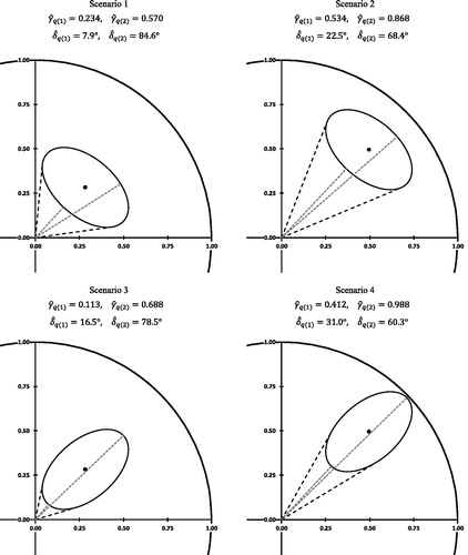
The second two lines indicate the points on the circumference of the confidence ellipse that are closest and farthest from the origin. The lengths of the corresponding vectors, ${\widehat{\gamma }}_{q(1)}$ and ${\widehat{\gamma }}_{q(2)}$, stand for the minimum and maximum distances of all points falling in the confidence ellipse to the origin, and their discrepancy therefore provides information about the precision of the estimate ${\widehat{\gamma }}_{1,q}$. As can be seen in Figure 4, the discrepancy between ${\widehat{\gamma }}_{q(1)}$ and ${\widehat{\gamma }}_{q(2)}$ depends on the shape and rotation of the confidence ellipse. Appendices B and C show how to compute the values of ${\widehat{\delta }}_{q(1)},\mathrm{ }{\widehat{\delta }}_{q(2)}$, ${\widehat{\gamma }}_{q\left(1\right),}$ and ${\widehat{\gamma }}_{q(2)}$.

Testing the differences of the locations of multiple covariates on a circumplex

The SPMC-E can be used to compare the locations of two or more covariates on the circumplex. For example, some research has investigated whether dark triad traits (i.e., narcissism, psychopathy, and Machiavellianism) occupy different positions on the IPC (e.g., Dowgwillo & Pincus, 2017; Rauthmann & Kolar, 2013). Such questions can be investigated by imposing constraints on the parameters describing the common scores’ correlations with the covariates. For example, in the case of Q covariates, the hypothesis that all covariates are equally related to the circumplex implies that all parameters could be subjected to equality constraints (i.e., ${\gamma }_{\mathrm{0,1}}=\dots ={\gamma }_{0,Q}$, ${\gamma }_{\mathrm{1,1}}=\dots ={\gamma }_{1,Q}$, and ${\delta }_1=\dots ={\delta }_Q$) without significantly reducing the model-data fit of the SPMC-E. Of course, by using this approach, researchers could also investigate more specific hypotheses that focus on the specific parameters (e.g., imposing equality constraints on only the $\delta$- or ${\gamma }_1$-parameters).

A simulation study

In order to further compare the SPMC-E to the SSM and the CIRCUM-extension, we conducted a small simulation study. The first issue investigated was the differences between the results obtained by the SSM, the CIRCUM-extension, and the SPMC-E. Here, we examined the agreement of estimates and the known relationships of a latent circumplex with a covariate. In situations where researchers are interested in a covariate’s relationship with a latent circumplex, discrepancies between results and true relationships can be considered as a form of bias. The second issue considered was the accuracy of inferences about the covariate’s relationship with the latent circumplex. To this end, we examined the standard error bias, and the proportion of replications in which confidence intervals and confidence ellipses included the true data generating parameters (coverage rates). Finally, we looked at the Type-I error rates that erroneously indicate that a covariate has a nonzero content specificity.

The SPMC-E was taken as the data generating model. We simulated eight circumplex indicators and one covariate. Data were generated for three conditions that reflected different degrees of the covariate’s content sensitivity (${\gamma }_1$-parameters). To provide a realistic scenario, we first analyzed the norm sample of the frequently used Interpersonal Adjective Scales (IAS; Wiggins, 1995) to derive the angular location of the eight types of interpersonal behavior and the shape of the SPCM’s correlation function. The locations of the common scores deviated somewhat from a perfect circumplex. Because the level component of the correlation function was close to zero, and other instruments typically have nonzero level components (e.g., Gurtman, 1992b), we set ${\beta }_0$ to a somewhat higher value. The correlation function used in this simulation, including the corresponding $\beta$-parameters, is depicted in the second panel of Figure 2. The average of the indicators’ squared communalities was set to .70.

The covariate’s content sensitivity was set to different values in each condition, namely, ${\gamma }_{1,q}$ = .70, ${\gamma }_{1,q}$ = .35, and ${\gamma }_{1,q}$ = .00, standing for a strong, medium, and absent content sensitivity, respectively. The remaining parameters of the model’s extension part did not differ between conditions (${\gamma }_{0,q}$ = .70 and ${\delta }_q$ = 135° in conditions one and two, respectively, and ${\delta }_q$ being undefined in condition three). Finally, $R_{D,q}^2$ was set to $R_{D,q}^2$ = .10 in all conditions, whereas $R_{F,q}^2$ differed between conditions because of the differences in the covariate’s content sensitivity. Details about the population parameters are reported in Appendix D.

For each condition, 500 replications with a sample size of N = 500 cases were drawn. The simulation was carried out with the Mplus 7.4 program (Muthén & Muthén, 1998–2010) by using conventional maximum likelihood estimation. We do not report results pertaining to the stand-alone SPMC. In a nutshell, the SPMC’s parameters were unbiased, had good parameter recovery rates, and had accurate standard errors. Detailed results are given in the supplementary material of this article.

Results

Parameter recovery

We start by reporting the results that pertain to the models’ estimates of the covariate’s average correlations, its content sensitivity, and its angular location. In order to make the estimates given by the CIRCUM-extension and the SPMC-E comparable to the estimates ${\widehat{g}}_{0,q}$ and ${\widehat{g}}_{1,q}$, given by the SSM, for the CIRCUM-extension we report the estimates ${\widehat{h}}_q{\widehat{\beta }}_0^2$ and ${\widehat{h}}_q\left(1-{\widehat{\beta }}_0^2\right)$ and, for the SPMC-E, the estimates ${\widehat{\gamma }}_{0,q}{\widehat{\beta }}_0^2$ and ${\widehat{\gamma }}_{1,q}\left(1-{\widehat{\beta }}_0^2\right)$. The results are presented in Table 2.

Table 2. Data generating parameter values and average estimates of the level component, the content sensitivity, and the angular location of the covariate’s location on the circumplex.

	Condition 1		Condition 2		Condition 3
	Pop.	M(Est.)	Pop.	M(Est.)	Pop.	M(Est.)
Level
SSM	.105	.111	.105	.104	.105	.098
CIRCUM-extension	.105	.104	.105	.060	.105	.024
SPMC-E	.105	.104	.105	.104	.105	.104
Content Sensitivity
SSM	.595	.411	.297	.206	.000	.042
CIRCUM-extension	.595	.592	.297	.338	.000	.136
SPMC-E	.595	.591	.297	.298	.000	.057
Angular Location
SSM	135°	141.7°	135°	142.0°	----	297.8°
CIRCUM-extension	135°	135.2°	135°	135.7°	----	163.5°
SPMC-E	135°	135.2°	135°	135.0°	----	281.0°

The SSM provided quite accurate estimates of the covariate’s average correlations but it clearly underestimated the covariate’s content sensitivity in conditions one (−30.9%) and two (−38.2%). However, in condition three, the SSM correctly indicated a content sensitivity close to zero. The estimates of the covariate’s angular location deviated, on average, by around 7° from the data generating values in conditions one and two. The angular location provided in condition three should not be interpreted because ${\widehat{d}}_q$ was quite uniformly distributed across replications, as shown in Figure 5.

Figure 5. Distribution of estimates of the covariate’s angular locations estimated by the SSM, the CIRCUM-extension, and the SPMC-E in Condition 3.

The CIRCUM-extension provided unbiased results in condition one. In condition two, the model still provided an accurate estimate of the angular location ${\delta }_q$, but it clearly underestimated the level component (−42.9%) and overestimated the content specificity (13.6%). The same pattern was observed in condition three, where the bias was even more severe (−77.1% in the case of the level component; percentage of bias for the content specificity is not defined). In the third condition, the CIRCUM-extension also provided biased results for the angular location because, as shown in Figure 5, this parameter tended to be estimated most often near 135°, although it was not defined in the population.

Finally, the SPMC-E provided virtually unbiased estimates for all parameters in all conditions. Again, the circular mean of the $\delta$-parameter in the third condition should not be interpreted because it was quite uniformly distributed (Figure 5).

Accuracy of inferences about the covariate’s relationship with the circumplex

Table 3 provides information about the variability of the sampling distribution of the level components of the covariate’s associations, as well as the Cartesian coordinates of the covariate’s location on the circumplex (i.e., SDs across replications, average standard errors of estimates, and percentage of standard error bias). In addition, it includes the areas of the confidence ellipses that were derived on the basis of the (co-)variation across replications (column SD), the areas derived on the basis of the parameters’ standard errors and their correlation [column M(SE)], as well as the percentage of bias of the latter areas (column SE-Bias). Table 3 also includes the coverage rates that refer to the proportion of replications in which the 95% confidence intervals (or ellipses) included the data generating values.

Table 3. Variability of estimates across replications, average standard errors, percentage standard error bias, and 95% coverage rates.

	Condition 1				Condition 2				Condition 3
	SD	M(SE)	SE-Bias	Cover.	SD	M(SE)	SE-Bias	Cover.	SD	M(SE)	SE-Bias	Cover.
SSM
${\widehat{g}}_{0,q}$	.015	.015	3.8%	.942	.015	.015	4.4%	.962	.016	.016	4.8%	.922
${\widehat{g}}_{1,q}\text{cos}\left({\widehat{d}}_q\right)$	.029	.029	−0.6%	.088	.032	.032	−0.6%	.652	.033	.033	0.5%	.946
${\widehat{g}}_{1,q}\text{sin}\left({\widehat{d}}_q\right)$	.032	.031	−4.3%	.000	.034	.033	−3.2%	.272	.034	.034	−2.1%	.940
Area	.017	.016	−4.6%	.000	.021	.020	−3.9%	.198	.021	.021	−1.7%	.942
CIRCUM-Extension
${\widehat{h}}_q$	.028	.025	−11.6%	.922	.042	.040	−3.7%	.000	.050	.048	−3.9%	.000
${\widehat{h}}_q\text{cos}\left({\widehat{\delta }}_q\right)$	.039	.029	−27.2%	.866	.045	.041	−9.6%	.824	.112	.049	−56.4%	.442
${\widehat{h}}_q\text{sin}\left({\widehat{\delta }}_q\right)$	.036	.028	−23.9%	.870	.043	.039	−8.3%	.858	.104	.047	−54.2%	.542
Area	.024	.015	−64.7%	.828	.036	.030	−20.4%	.792	.219	.043	−407.0%	.262
SPMC-E
${\widehat{\gamma }}_{0,q}$	.104	.104	−0.9%	.936	.122	.121	−1.4%	.948	.127	.131	3.1%	.950
${\widehat{\gamma }}_{1,q}\text{cos}\left({\widehat{\delta }}_q\right)$	.045	.045	−0.0%	.946	.050	.049	−0.7%	.938	.056	.056	0.7%	.954
${\widehat{\gamma }}_{1,q}\text{sin}\left({\widehat{\delta }}_q\right)$	.039	.040	−0.6%	.946	.045	.045	−0.6%	.946	.055	.056	0.9%	.954
Area	.030	.031	1.6%	.942	.042	.041	−2.0%	.950	.057	.054	−6.0%	.954

Note. Area = Area of the confidence ellipse; SD of Area = Area on the basis of (co-)variation across replications, M(SE) of Area = Average area based on the (co-)variances of estimates, Coverage of Area = Proportion of replications in which the 95% confidence area includes the covariate’s location.

The results for the SSM can be summarized as follows. The standard errors of all coefficients were found to be accurate in all conditions. Only the estimate ${\widehat{g}}_{0,q}$ was found to generally exhibit satisfactory coverage rates because this coefficient was found to be relatively unbiased (Table 2). In contrast, the coverage rates for the x- and y-coordinates, as well as the confidence ellipse of the covariate’s location on the circumplex, had poor coverage rates in conditions one and two because the covariate’s content specificity was systematically underestimated (Table 2). However, in condition three, where the covariate was not content sensitive, coverage rates were good. Here, the Type-I error rate of the confidence ellipse was close to the nominal value of .05 (i.e., 1 − .942 = .058).

The CIRCUM-extension produced unsatisfactory results. All standard errors and the area of the confidence ellipse were negatively biased in condition one. The standard errors of ${\widehat{h}}_q$ were very close to the corresponding standard deviations in conditions two and three, but coverage rates were essentially zero because the parameter was strongly biased (Table 1). In addition, the uncertainty of the covariate’s location was underestimated in conditions two and three and this resulted in poor coverage rates. Most importantly, in condition three, the confidence ellipse included the origin of the circumplex only in 26.2% of the replications, which means that the Type-I error rate was 1 − .262 = .738. Finally, the SPMC-E provided accurate standard errors, confidence ellipses, and coverage in all conditions. As a consequence, the Type-I error rates derived in condition three were very close to the nominal value (i.e., 1 − .954 = .046).

Accuracy of relationships of unique variables and of interval estimates provided by the SPMC-E

Here we focus on the covariate’s associations with the unique factors and on the interval estimates ${\widehat{\delta }}_{q(1)}$ and ${\widehat{\delta }}_{q(2)}$, and ${\widehat{\gamma }}_{q(1)}$ and ${\widehat{\gamma }}_{q(2)},$ given by the SPMC-E. The interval estimates derived on the basis of the SSM and CIRCUM-extension were not further considered because of the poor coverage rates of their confidence ellipses (Table 3).

The correlations of the unique factors with the covariate are presented in Table 4. Unique correlations were generally well recovered, and their standard errors were in good agreement with the standard deviations of the estimates. As a consequence, the coverage rates of the unique correlations were satisfactory. Table 5 presents the results for the squared multiple correlations of common factors ($R_{F,q}^2$), unique factors ($R_{D,q}^2$), and their sum ($R_q^2$). As can be seen, the squared multiple correlations of common factors had a good recovery, whereas $R_{D,q}^2$ was, on average, slightly overestimated. This result was not unexpected because, due to their squared nature, positive and negative deviations from the population values cannot cancel out across replications. Finally, Table 5 compares the lower and upper bounds, ${\widehat{\delta }}_{q(1)}$ and ${\widehat{\delta }}_{q(2)}$, and ${\widehat{\gamma }}_{q(1)}$ and ${\widehat{\gamma }}_{q\left(2\right),}$ which were averaged across replications with the values that were computed on the basis of the (co-)variation of the parameter estimates across replications. The average lower and upper bounds of both sets of parameters had an almost perfect agreement.

Table 4. Data generating parameter values, average estimates, standard deviations across replications, and 95% coverage rages of correlations of unique factors estimated by the SPMC-E.

	Condition 1					Condition 2				Condition 3
	Pop.	M(Est.)	SD	M(SE)	Cover.	M(Est.)	SD	M(SE)	Cover.	M(Est.)	SD	M(SE)	Cover.
LM	−0.062	−0.062	0.035	0.034	0.950	−0.058	0.041	0.041	0.954	−0.060	0.049	0.061	0.970
NO	0.194	0.197	0.041	0.043	0.970	0.196	0.049	0.051	0.962	0.195	0.045	0.055	0.964
PA	−0.093	−0.090	0.042	0.045	0.968	−0.095	0.045	0.049	0.970	−0.086	0.044	0.059	0.980
BC	0.012	0.016	0.046	0.047	0.926	0.017	0.039	0.040	0.940	0.015	0.043	0.056	0.982
DE	−0.093	−0.090	0.040	0.040	0.960	−0.094	0.040	0.042	0.962	−0.093	0.045	0.060	0.980
FG	0.195	0.199	0.043	0.044	0.964	0.197	0.050	0.052	0.958	0.194	0.043	0.055	0.986
HI	−0.048	−0.044	0.042	0.040	0.956	−0.039	0.049	0.049	0.962	−0.047	0.045	0.057	0.976
JK	−0.023	−0.031	0.037	0.035	0.936	−0.030	0.034	0.034	0.954	−0.025	0.042	0.056	0.986

Table 5. Lower and upper values of interval estimates of the covariate’s content sensitivity (${\gamma }_1$) and orientation ($\delta$), and proportion of variance shared with unique factors ($R_{D,q}^2$), common factors ($R_{F,q}^2$), and all factors ($R_q^2$) derived by the SPMC-E.

	Condition 1		Condition 2		Condition 3
	Pop.	M(Est.)	Pop.	M(Est.)	Pop.	M(Est.)
${\widehat{\gamma }}_{1,q(1)}$	.621	.613	.237	.236
${\widehat{\gamma }}_{1,q(2)}$	.779	.778	.464	.465
${\widehat{\delta }}_{q(1)}$	124.8°	124.9°	114.7°	114.7°
${\widehat{\delta }}_{q(2)}$	144.9°	145.0°	154.0°	153.9°
$R_q^2$	.590	.600	.278	.297	.174	.194
$R_{F,q}^2$	.490	.486	.178	.181	.074	.080
$R_{D,q}^2$	.100	.115	.100	.117	.100	.114

Notes. Interval estimates are not defined in Condition 3.

Population Values of Interval Estimates are Based on the (Co-)Variation of Parameter Estimates Across Replications.

Summary

The simulation study gave a first insight into the usefulness of the SPMC-E. Although the study is limited, its results are encouraging. The SPMC-E produced accurate (i.e., unbiased) estimates in all conditions. Furthermore, the model gave accurate estimates of the key parameters’ (co-)variances, as it provided accurate estimates of the confidence ellipse of a covariate’s location on the circumplex. The interval estimates for the $\delta$- and ${\gamma }_1$-parameters had a high accuracy and Type-I error rates were close to the nominal values.

The results document that, when the data are generated by the SPMC-E, the SSM underestimates the covariate’s content specificity (conditions one and two). The main reason for this result is the fallible nature of indicator variables. In addition, the results indicate that failing to account for the unequal spacing of circumplex indicators affects the estimate of the covariate’s angular location (see also the results provided on the basis of Gurtman’s, 1992b data). However, discrepancies between the SSM’s results and population generating parameters cannot be interpreted entirely as bias, because the SPMC-E used to generate the data incorporates a different identification strategy (minimum sum of squares of correlations of unique factors) than the SSM (minimum sum of squares of discrepancies between sample correlations and fitted correlations). Nevertheless, additional analyses in which we fixed the circumplex variable’s angular locations to the population values resulted in estimates that were much closer to 135°. This result supports the assumption that the incorrect specification of the indicators’ angular locations is the main factor responsible for the observed discrepancy of the estimated covariates’ angular location.

Finally, the CIRCUM-extension provided reasonable parameter estimates only in the condition in which the covariate had the same sensitivity for the level and scatter component of the SPCM’s correlation function as the circumplex indicators. In conditions two and three, which violated this assumption, the CIRCUM-extension provided results that are very likely to lead to wrong conclusions. Even in the optimal case (condition one), the CIRCUM-extension did not provide accurate inferences because the standard errors underestimated the parameters’ sampling variability.

Empirical illustration of the new extension procedure

In this section, we provide an empirical illustration of the SPMC-E that draws on the IPC (Wiggins, 2003) that was assessed by a German adaption of the IAS (Jacobs & Scholl, 2005). In this application, the SPMC was extended to include two measures of narcissistic personality styles, differentiating between narcissistic admiration and rivalry (Back, Küfner, Dufner, Gerlach, Rauthmann, & Denissen, 2013). The admiration and rivalry dimensions are assumed to reflect two strategies for maintaining a grandiose self, namely, self-enhancement (admiration) and self-defense (rivalry). The self-defense path is thought to be related to social interaction styles that are likely to lead to higher levels of interpersonal conflicts, whereas the self-enhancement pathway is hypothesized to be motivated by the desire for social interactions that lead to popularity (Küfner, Nestler, & Back, 2013). Hence, the two aspects of narcissism can be expected to be related to the IPC, but to occupy different locations on the IPC. More specifically, it seems plausible that the admiration aspect is most strongly related to dominant types of interpersonal behavior (PA; Figure 1), and the rivalry dimension is more strongly related to coldhearted interpersonal behavior types (DE and BC; Figure 1).

All analyses were run with the Mplus 7.4 program (Muthén & Muthén, 1998–2010), using the conventional maximum likelihood estimator. Mplus input files are available in the online supplement of this article. Model fit was evaluated with respect to the χ² statistic, the comparative fit index (CFI; Bentler, 1990), the root mean error of approximation (RMSEA; Browne & Cudeck, 1993), and the standardized root mean square residual (SRMR; Jöreskog & Sörbom, 1993). The fit of nested models was compared by means of the χ²-difference test.

Sample and results

The data stem from a recent online study. Here, we included those N = 688 participants who had complete data on the measures of the IAS and the Narcissistic Admiration and Rivalry Questionnaire (NARQ; Back et al., 2013). Table 1 presents the descriptive statistics for the IAS and NARQ instruments.

We first applied the SPMC to the IAL. A model with M = 3 components gave the best fit to the IAS data [χ² (df = 10) = 69.53, p < .001; RMSEA = .093; CFI = .982; SRMR = .090]. All $\beta$-parameters were statistically significant at the level of p < .001. The right panel of Figure 2 provides the estimated correlation function, showing that the level component was close to zero (${\widehat{\beta }}_0^2$ = 0.14), so that the correlation function was highly scattered with a maximum of ${\widehat{\beta }}_1^2+{\widehat{\beta }}_2^2+{\widehat{\beta }}_3^2$ = 0.86 points above the level, and a minimum of ${\widehat{\beta }}_1^2-{\widehat{\beta }}_2^2+{\widehat{\beta }}_3^2$ = 0.81 points below the average correlation. The remaining parameters are given in Table 6. All scaling constants were significant, but the variables LM and JK had smaller parameter values. Communality estimates were high on average, with the smallest value being determined for JK. This result was mirrored in the unique factor loadings. Finally, the angular locations of the common scores showed a high correspondence to their theoretical positions (Figure 1).

Table 6. Parameters of the SPMC Applied to the IAL Instrument.

	${\widehat{\zeta }}_{x_j}$	(SE)	${\widehat{\theta }}_j$	(SE)	${\widehat{\nu }}_j$	(SE)	${\widehat{h}}_j^2$
LM	0.863	(0.031)**	0.0°	(-.--)	0.365	(0.057)**	.882
NO	0.905	(0.027)**	48.3°	(2.0°)	0.201	(0.077)**	.961
PA	1.014	(0.033)**	98.2°	(2.7°)	0.458	(0.045)**	.827
BC	1.063	(0.038)**	148.3°	(2.4°)	0.464	(0.044)**	.823
DE	0.950	(0.033)**	179.6°	(2.1°)	0.496	(0.044)**	.802
FG	1.070	(0.036)**	222.8°	(2.5°)	0.517	(0.040)**	.789
HI	1.121	(0.033)**	272.0°	(2.5°)	0.188	(0.088)*	.966
JK	0.753	(0.033)**	309.1°	(2.7°)	0.774	(0.051)**	.625

Note: $\widehat{\zeta }$ = estimated scaling parameters, $\widehat{\theta }$ = estimated angular locations, $\widehat{\nu }$ = estimated unique factor loadings, ${\widehat{h}}^2$ = estimated communality indexes.

* p < .05;

** p < .01.

The model was extended to the SMPC-E by including the admiration and rivalry aspects of narcissism in the analysis.⁶ As shown in Table 7, both covariates shared a substantial proportion of variance with the IAS circumplex (admiration: 35%, rivalry: 54%). The bulk of shared variance was due to the common factors (admiration: 34%, rivalry: 49%). This result supports the validity of interpreting both covariates’ positions on the circumplex, although the admiration scale showed a better fit to the model. This interpretation was confirmed by the results of nested model comparisons. Fixing the correlations between the unique factors and the admiration scale to zero did not result in a significant decrement in model fit [Δχ² (df = 5) = 10.33, p = .067], but the comparison was statistically significant in the case of the rivalry scale [Δχ² (df = 5) = 28.64, p < .001].

Table 7. Parameters of the extension part of the SPMC-E applied to the interpersonal circumplex and narcissism scales.

	Admiration	Rivalry
	Est. (SE)	Est.(SE)
Proportion of Shared Variance
Common Factors	.338	.491
Unique Factors	.015	.052
Total	.352	.543
Correlations of Unique Factors
LM (Warm-Agreeable)	0.013 (0.047)	0.124 (0.041)**
NO (Gregarious-Extraverted)	−0.013 (0.025)	−0.092 (0.033)**
PA (Assured-Dominant)	0.030 (0.045)	0.018 (0.040)*
BC (Arrogant-Calculating)	−0.072 (0.033)*	0.117 (0.037)**
DE (Coldhearted)	0.088 (0.036)*	−0.013 (0.034)
FG (Aloof-Introverted)	−0.013 (0.039)	−0.111 (0.039)**
HI (Unassured-Submissive)	−0.009 (0.019)	0.021 (0.023)
JK (Unassuming-Ingenuous)	0.012 (0.035)	−0.035 (0.032)
Relationships with the Latent Circumplex
Level (${\widehat{\gamma }}_{0,q}$)	0.802 (0.092)**	0.758 (0.087)**
Content Sensitivity (${\widehat{\gamma }}_{1,q}$)	0.538 (0.033)**	0.691 (0.035)**
[${\widehat{\gamma }}_{1,q(1)}$; ${\widehat{\gamma }}_{1,q(2)}$]	[0.458; 0.617]	[0.623; 0.759]
Angular Location (${\widehat{\delta }}_q$)	101.9° (4.7°)	179.7° (3.5°)
[${\widehat{\delta }}_{q(1)}$; ${\widehat{\delta }}_{q(2)}$]	[90.2°; 113.2°]	[171.2°; 188.2°]

Notes: ${\widehat{\gamma }}_{0,q}$ = estimate of level component of external common score correlations, ${\widehat{\gamma }}_{1,q}$ = estimate of a covariate’s content sensitivity, ${\widehat{\gamma }}_{1,q(1)}$ and ${\widehat{\gamma }}_{1,q(2)}$ = lower and upper bounds of content sensitivity, respectively, ${\widehat{\delta }}_q$ = estimate of angular location, ${\widehat{\delta }}_{q(1)}$ and ${\widehat{\delta }}_{q(2)}$ = lower and upper bounds of angular location, respectively.

* p < .05;

** p < .01.

Figure 6 provides an insight into the fit of the pattern of associations of IAS scores with the covariates to the shape of the SPMC’s correlation function. In this figure, the covariance between the rescaled IAS scores (i.e., $x^{*}$-variables) and the rescaled admiration and rivalry scores (i.e., $y^{*}$-variables), ${\sigma }_{y_q^{*},x_j^{*}}$, is decomposed into parts that are compatible with Equation 16(16) $${\rho }_{c_j,y_q^{*}}={\gamma }_{0,q}{\beta }_0^2+{\gamma }_{1,q}\sum _{m=1}^M{\beta }_m^2\text{cos}\left[\begin{array}{c}m\left({\theta }_j-{\delta }_q\right)\end{array}\right] ,$$(16) , ${\rho }_{c_j,y_q^{*}}$, and parts that represent deviations thereof, ${\nu }_{x_j^{*}}{\rho }_{y_q^{*},u_j}$ (Equation 21(21) $${\sigma }_{y_q^{*},x_j^{*}}={\rho }_{c_j,y_q^{*}}+{\nu }_j{\rho }_{y_q^{*},u_j}$$(21) ). The deviations were very small for the admiration scale and were somewhat larger for the rivalry scale.

Figure 6. Upper panel: Location of admiration and rivalry scales on the IAS circumplex, including 95% confidence ellipses determined by the SPMC-E. Lower panels: Correlation functions (solid lines) and covariances (open circles) between scaled IAL scores and admiration (left panel) and rivalry (right panel) scales. LM = Warm-Agreeable, NO = Gregarious-Extraverted, PA = Assured-Dominant, BC = Arrogant-Calculating, DE = Coldhearted, FG = Aloof-Introverted, HI = Unassured-Submissive, JK = Unassuming-Ingenuous.

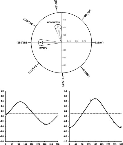
An observation that can be made from Figure 6 is that the profiles of correlations pertaining to the admiration and rivalry scales appear to have the same overall level (see also estimates ${\widehat{\gamma }}_{0,Adm}$ and ${\widehat{\gamma }}_{0,Riv}$ in Table 3). Additional analyses indicated that these coefficients did not differ significantly from each other [Δχ² (df = 1) = 0.20, p = .657]. In contrast, the results indicated that the relationships of the rivalry variable were more strongly scattered (see also estimates of ${\widehat{\gamma }}_{1,Adm}$ and ${\widehat{\gamma }}_{1,Riv}$ in Table 3). Furthermore, as shown in Table 6, the range covered by the minimum and maximum values of these estimates, constructed on the basis of the 95% confidence ellipse, did not overlap, thus suggesting a statistically significant difference. This interpretation was confirmed by a χ²-difference test [Δχ² (df = 1) = 15.01, p < .001]. Finally, the results suggested that the angular locations of the admiration and rivalry scales differed significantly from each other. As shown in Figure 6, admiration was closest to the PA scale of the IAS (assured-dominant) at ${\widehat{\delta }}_{Adm}$ = 101.9°, whereas rivalry (${\widehat{\delta }}_{Riv}$ = 179.7°) was closest to the DE scale of the IAS (coldhearted). The fact that the confidence ellipses did not overlap suggests that the locations were significantly different from each other, a result that was confirmed by a model comparison [Δχ² (df = 1) = 190.16, p < .001].

Summary

The analyses reported here demonstrate the capability of the SMPC-E to investigate a variety of theoretically relevant hypotheses and to assess the precision of the parameters by which covariates are mapped onto a circumplex. Our real-data example provided sound evidence that the admiration and rivalry aspects of narcissistic personality types, as measured with the NARQ, are both strongly related to the IPC, as measured with the IAS. The admiration aspect was better aligned to the SPMC’s correlation function, but its relationship with the IAL was somewhat weaker compared to the rivalry scale. Most importantly, our analyses provide clear evidence that admiration and rivalry occupy different locations on the IAL circumplex and differ in their sensitivity to the IPC’s interpersonal content.

Summary and discussion

In recent years, the SPMC (Browne, 1992) has gained widespread popularity as a powerful and flexible method for examining circumplex structures. However, up until now, the flexibility of the framework provided by the SPMC was limited to the examination of circumplex structures. As a consequence, most researchers interested in the relationships of a circumplex with covariates utilized the SSM (Gurtman & Pincus, 2003). The SSM is not a latent variable model, which means that it does not provide estimates for the covariates’ associations with a latent circumplex – something that is of interest in many research settings. As an alternative to the SSM, the CIRCUM-extension (Yik & Russel, 2004) has been suggested as a method that allows covariates to be related to a latent circumplex as modeled by the SPMC. This model builds on the strong assumption that covariates can be treated as indicators of the circumplex. As it is likely that this assumption will not be met in many situations, it limits the method’s generalizability.

Our suggested extension of the SMPC, the SPMC-E, makes it possible to investigate the relationships between a latent circumplex and covariates in one coherent framework that offers great flexibility. Our method combines the strengths of the SSM and the CIRCUM-extension because (1) it relates covariates to a latent circumplex instead of to observed variables, (2) it ensures that the shape of the profiles of the covariates’ relationships with the common scores of the circumplex indicators adheres to the shape of the circumplex correlation function, and (3) it allows covariates to be differently related to the level and the content sensitivity of the latent circumplex. Furthermore, the SPMC-E (4) provides interval estimates of the parameters that allow covariates to be located on a latent circumplex, and (5) makes it possible to test a variety of hypotheses about the covariates’ relationships with a circumplex.

In the applications of the SPMC-E to real datasets, we documented its potential for examining the nomological net of relationships of a circumplex (Gurtman, 1992a). The second empirical study provides an example of a construct map in which covariates placed on a circumplex were supplemented with confidence ellipses. Furthermore, the fact that the SPMC-E is specified in the context of SEM allows researchers to test a variety of hypotheses, such as testing for differences between the covariates’ content sensitivity and their angular locations. This capability of the SPMC-E is of relevance in all fields of psychology where circumplex models are proposed, such as vocational interests (Tracey & Rounds, 1993), affect (Watson et al., 1999), and values (Schwartz, 1992).

Comparison of the SPCM-E with the SSM and the CIRCUM-Extension

The SPMC-E appears as a method of choice when covariates are to be related to a circumplex that is considered as a latent structure to be modeled in a flexible framework. However, as the model shares some similarities with the SSM and the CIRCUM-extension, the question emerges about applications for which the latter two approaches are more attractive than the SPMC-E.

The strength of the SSM is that it is easy to apply, as it does not include latent variables and does not require specialized software to be estimated. As such, the SSM provides a quick overview of the locations of multiple covariates on a circumplex and can be used even in small samples, where latent variable models that are based on maximum likelihood estimation techniques can no longer be reliably applied. We expect the SSM to provide reasonable estimates of the covariates’ angular locations when good approximations to the true angular locations of the circumplex indicators are available, and when the size of the indicators’ unique components is not systematically related to their circumplex locations (as was the case in our simulation study). A drawback of the model is that the content sensitivity of the covariates will be generally underestimated because circumplex indicators will almost always include a unique component. We also found that deviations of a covariate’s relationships from the cosine function could affect the estimates, but the impact was rather small (results are not reported). Nevertheless, this issue warrants further attention. When the aforementioned preconditions are met, it might even be the case that the SSM provides good interval estimates of the covariates’ angular locations, either on the basis of the confidence ellipse or based on the resampling procedure suggested by Zimmermann and Wright (2017). More research is needed before specific recommendations can be given.

The CIRCUM-extension is attractive in applications that aim to identify the common parts of the covariates that can be placed together with the circumplex indicators’ common parts on the perimeter of a circle (e.g., Yik & Russell, 2001; Yik, Russell, Oceja, & Dols, 2000). In order to do so, the covariates are subjected to the same measurement model that is applied to the indicators of the circumplex. This is a difference to the SPMC-E, which includes only a linear transformation of covariates. Nevertheless, both models are closely related to each other. When they are estimated by the two-step approach, the CIRCUM-extension is nested in the SPMC-E because it constrains the $\gamma$-parameters attached to the covariate $y_q$ to ${\gamma }_{0,q}={\gamma }_{1,q}=h_q$. Therefore, when the SPMC-E is estimated in a single step, it can be used to evaluate whether the constraint imposed in the CIRCUM-extension is compatible with the minimum sum of squares criterion applied to the correlations of the unique factors. If this hypothesis turns out to be compatible with the data, and the equality constraint is imposed on the $\gamma$-parameters, the SPMC-E delivers a communality index and an angular location that has the same meaning as the parameters provided by the CIRCUM-extension. Therefore, the SPMC-E can be used to locate a covariate’s common part on a circumplex and to accompany its location with a sound interval estimate. As we have shown, the CIRCUM-extension does not deliver realistic interval estimates, even in ideal conditions. In addition, when covariates do not have the same properties as circumplex indicators, the CIRCUM-extension is very likely to lead to wrong conclusions; a risk that can be avoided by using the SPMC-E.

Future developments

Even though we have attempted to provide an approach suitable for a wide area of applications, our procedure is not without limitations. For example, more knowledge about the robustness of results across a variety of situations commonly encountered in practice is needed (e.g., presence of missing data, violations to multivariate normality and to independent sampling). Of course, as the SPMC and its extension belong to the class of CFA models, the options provided by many SEM packages for dealing with these issues, can also be applied to the SPCM-E. However, the SPMC-E has a complex loading structure that is subjected to multiple nonlinear constraints. To the best of our knowledge, the performance of such models has not yet been scrutinized in depth.

The variables assessed in the social sciences are often gathered via Likert scales, which means that they are ordinal rather than continuous. A common way of handling this issue is to aggregate multiple items, as done in our empirical example, so that the variables are better aligned to a continuous scale (e.g., Hau & Marsh, 2004). In situations where only single items are available, this approach is no longer feasible. In recent years, estimation techniques for ordinal data have been implemented in SEM programs (Muthén, 1984). The SPMC-E can be combined with measurement models for ordinal data (e.g., the graded response model) and estimated via limited information estimators that can handle high dimensional models. Up until today, the estimation of circumplex models by these estimators has not been studied, although this issue deserves more attention.

The SPMC and the SPMC-E can be estimated by SEM computer programs; in our opinion, Mplus (Muthén & Muthén, 1998–2010) and MX (Neale et al., 2016) appear to be the most convenient because they allow parameters to be constrained according to trigonometric functions (see the online supplement for the Mplus code). However, we recognize that the setup of the SPMC and SPMC-E is quite demanding for users with just a basic background in SEM programing. Therefore, in order to disseminate the method to a broader audience, we are currently working on an Mplus interface that enables a more user-friendly specification and estimation of the SMPC-E, including the confidence ellipses and interval estimates introduced in this article.

Article Information

Conflict of interest disclosures: Each author signed a form for disclosure of potential conflicts of interest. No authors reported any financial or other conflicts of interest in relation to the work described.

Ethical principles: The authors affirm having followed professional ethical guidelines in preparing this work. These guidelines include obtaining informed consent from human participants, maintaining ethical treatment and respect for the rights of human or animal participants, and ensuring the privacy of participants and their data, such as ensuring that individual participants cannot be identified in reported results or from publicly available original or archival data.

Funding: This work was not supported by a grant.

Role of the funders/sponsors: None of the funders or sponsors of this research had any role in the design and conduct of the study; collection, management, analysis, and interpretation of data; preparation, review, or approval of the manuscript; or decision to submit the manuscript for publication.

Acknowledgments: The authors would like to thank Gráinne Newcombe and Alexander Robitzsch for their comments on prior versions of this manuscript. The ideas and opinions expressed herein are those of the authors alone, and endorsement by the authors’ institutions is not intended and should not be inferred.

Notes

1 In the case of M = 1, Equations 1 and 2 imply a factor model in which a standardized indicator variable reflects three uncorrelated common factors $F_0$, $F_C$, and $F_S$ as $x_j=\mathrm{ }{\lambda }_{j,0}{F}_0+{\lambda }_{j,C}{F}_C+{\lambda }_{j,S}{F}_S+E_j$. The loadings are functions of the SPMC’s parameters: ${\lambda }_{j,0}=h_j{\beta }_0$, ${\lambda }_{j,C}=h_j{\beta }_1\text{cos}\left({\theta }_j\right)$, and ${\lambda }_{j,S}=h_j{\beta }_1\text{sin}\left({\theta }_j\right)$ (Nagy et al., 2009). When the indicators’ communalities are close to each other, and the model fits the data to a sufficient degree, the loadings ${\lambda }_{j,C}$ and ${\lambda }_{j,S}$ will be close (up to a rotation) to the loadings provided by an exploratory factor analysis. Therefore, the SPMC is closely related to the traditional factor analytic approach to the circumplex. In addition, the SPMC extends the traditional approach by accommodating situations where additional factors are required to model a circumplex correlation structure (by increasing the number of components M).

2 The coefficients of the SSM are typically derived on the basis of a reformulated model that can be written as a linear regression: ${\rho }_{x_j{y}_q}=g_{0,q}+b_{c,q}\text{cos}\left({\theta }_j\right)+b_{s,q}\text{sin}\left({\theta }_j\right)$ (e.g., Batschelet, 1981), where $b_{c,q}$ and $b_{s,q}$ are transformed to $g_{1,q}={\left(b_{c,q}^2+b_{s,q}^2\right)}^{1/2}$ and $d_q=\hspace{0.17em}{\text{tan}}^{-1}\left(b_{s,q}/b_{c,q}\right)$. As a linear model, the SSM includes residuals that refer to the discrepancy between sample correlations $r_{x_j{y}_q}$ and predicted correlations ${\rho }_{x_j{y}_q}$ ($e_j=r_{x_j{y}_q}-{\rho }_{x_j{y}_q}$) and that fulfil the requirements of least squares regression: ${\sum }_{j=1}^J{e}_j^2={\sum }_{j=1}^J{e}_j\text{cos}\left({\theta }_j\right)={\sum }_{j=1}^J{e}_j\text{sin}\left({\theta }_j\right)$ = 0.

3 By keeping the model parts for ${\mathit{\Sigma }}_{\mathit{y},\mathit{x}}$ and ${\mathit{\Sigma }}_{\mathit{y},\mathit{y}}$ just identified, we ensure that the value of the fit function employed is solely driven by the degree of approximation of ${\mathit{S}}_{\mathit{x},\mathit{x}}$ by ${\mathit{\Sigma }}_{\mathit{x},\mathit{x}}$ (Equations 6 and 7). Note that this does not mean that the matrices ${\mathit{\Sigma }}_{\mathit{y},\mathit{x}}$ and ${\mathit{\Sigma }}_{\mathit{y},\mathit{y}}$ correspond exactly to their sample counterparts ${\mathit{S}}_{\mathit{y},\mathit{x}}$ and ${\mathit{S}}_{\mathit{y},\mathit{y}}$ when maximum likelihood estimation techniques are employed. Such a result is only given when the SPMC has a perfect fit, which implies ${\mathit{\Sigma }}_{\mathit{x},\mathit{x}}={\mathit{S}}_{\mathit{x},\mathit{x}}$.

4 The parameter ${\gamma }_{1,q}$ has, by definition, a lower bound of zero, which means that it cannot be tested against zero with procedures that assume nearly normally distributed estimates. In the case of the angular parameter ${\delta }_q$, it can be argued that procedures developed for linear models cannot be applied directly to circular parameters (Batschelet, 1981).

5 Equation 32 can be modified to derive a Wald-${\chi }^2$ test of the null hypothesis that the location of a covariate equals a reference location. To this end, the terms ${\tilde{\varphi }}_{C,q}$ and ${\tilde{\varphi }}_{S,q}$ in Equation 31 need to be fixed to corresponding values (e.g., ${\tilde{\varphi }}_{C,q}={\tilde{\varphi }}_{S,q}=$ 0 in the case of the origin of the circumplex). Then, Equation 32 delivers a statistic that, in large samples, follows a ${\chi }^2$-distribution with df = 2.

6 Judged on the basis of the commonly used cut-off values of the RMSEA and the SRMR, the SPMC did not fit the data very well. This misfit can be propagated to the extension part of the SPMC-E because the parameters of the extension part describe the covariates’ relationships with the indicators implied by the SPMC, and not with the actual indicators. We investigated this issue by comparing the model-implied correlations between covariates and circumplex indicators with the corresponding sample correlations. Deviations were very small (admiration: MAD = .031, ranging from .007 to .055; rivalry: MAD = .031, ranging from .011 to .070). This means that the SPMC-E provided a good approximation of the covariates’ relationships despite its mediocre fit to the correlation pattern of circumplex indicators.

Appendix A: Construction of the confidence ellipse

Here, the construction of a confidence ellipse around the point estimates ${\widehat{\varphi }}_{C,q}={\widehat{\gamma }}_{1,q}\hspace{0.17em}\text{cos}\hspace{0.17em}\left({\widehat{\delta }}_q\right)$ and ${\widehat{\varphi }}_{S,q}={\widehat{\gamma }}_{1,q}\hspace{0.17em}\text{sin}\hspace{0.17em}\left({\widehat{\delta }}_q\right)$ via the parametric equation of the ellipse is outlined. To this end, the major and semi-axis of the ellipse, $a_q$ and $b_q$, need to be computed. The squares of these axes correspond to the eigenvalues of the covariance matrix of ${\widehat{\varphi }}_{C,q}$ and ${\widehat{\varphi }}_{S,q,}$ multiplied by ${\chi }_{2,\alpha }^2$, such that (A1) $$\begin{array}{c}{a}_q={\left\{{\chi }_{2,\alpha }^2\left[\frac{{\widehat{\sigma }}_{C,q}^2+{\widehat{\sigma }}_{S,q}^2}{2}+{\left(\frac{{\left({\widehat{\sigma }}_{C,q}^2-{\widehat{\sigma }}_{S,q}^2\right)}^2}{4}+{\widehat{\sigma }}_{C,q}^2{\widehat{\rho }}_{CS,q}^2{\widehat{\sigma }}_{S,q}^2\right)}^{1/2}\right]\right\}}^{1/2}\\ b_q={\left\{{\chi }_{2,\alpha }^2\left[\frac{{\widehat{\sigma }}_{C,q}^2+{\widehat{\sigma }}_{S,q}^2}{2}-{\left(\frac{{\left({\widehat{\sigma }}_{C,q}^2-{\widehat{\sigma }}_{S,q}^2\right)}^2}{4}+{\widehat{\sigma }}_{C,q}^2{\widehat{\rho }}_{CS,q}^2{\widehat{\sigma }}_{S,q}^2\right)}^{1/2}\right]\right\}}^{1/2}.\end{array}$$(A1)

In addition, the orientation of the major axis $a_q$ relative to the x-axis of the coordinate system is required. The orientation can be computed as follows: (A2) $${\omega }_q=\left\{\begin{array}{cccc}\frac{1}{2}\hspace{0.17em}{\text{tan}}^{-1}\left(\frac{2{\widehat{\sigma }}_{C,q}{\widehat{\rho }}_{CS,q}{\widehat{\sigma }}_{S,q}}{{\widehat{\sigma }}_{C,q}^2-{\widehat{\sigma }}_{S,q}^2}\right)& for& {\widehat{\rho }}_{CS,q}>0 ,& {\widehat{\sigma }}_{C,q}^2>{\widehat{\sigma }}_{S,q}^2\\ \frac{1}{2}\left[\hspace{0.17em}{\text{tan}}^{-1}\left(\frac{2{\widehat{\sigma }}_{C,q}{\widehat{\rho }}_{CS,q}{\widehat{\sigma }}_{S,q}}{{\widehat{\sigma }}_{C,q}^2-{\widehat{\sigma }}_{S,q}^2}\right)+\pi \right]& for& & {\widehat{\sigma }}_{C,q}^2<{\widehat{\sigma }}_{S,q}^2\\ \frac{1}{2}\left[\hspace{0.17em}{\text{tan}}^{-1}\left(\frac{2{\widehat{\sigma }}_{C,q}{\widehat{\rho }}_{CS,q}{\widehat{\sigma }}_{S,q}}{{\widehat{\sigma }}_{C,q}^2-{\widehat{\sigma }}_{S,q}^2}\right)+2\pi \right]& for& {\widehat{\rho }}_{CS,q}<0 ,& {\widehat{\sigma }}_{C,q}^2>{\widehat{\sigma }}_{S,q}^2\end{array}\right..$$(A2)

The parametric equations of the confidence ellipse provide the x- and y-coordinates of the circumference of the ellipse in a two-dimensional coordinate system, so that the points on the perimeter of the confidence ellipse are expressed as (A3) $$\begin{array}{c}{\tilde{\varphi }}_{C,q}={\widehat{\varphi }}_{C,q}+a_q\text{cos}\left({\omega }_q\right)\text{cos}\left(\phi \right)-b_q\text{sin}\left({\omega }_q\right)\text{sin}\left(\phi \right),\\ {\tilde{\varphi }}_{S,q}={\widehat{\varphi }}_{S,q}+a_q\text{sin}\left({\omega }_q\right)\text{cos}\left(\phi \right)+b_q\text{cos}\left({\omega }_q\right)\text{sin}\left(\phi \right)\end{array}\mathrm{ }$$(A3) where $\phi$ is a variable angle used for the purpose of plotting the ellipse (e.g., Batschelet,1981).

Appendix B: Closest and farthest distance to the confidence ellipse

Here, we explain a procedure for finding the closest and farthest distance from the origin of the coordinate system to the perimeter of the confidence ellipse, when the origin (0,0) of the coordinate system is outside the confidence ellipse. The squared distance from the origin to a point on the circumference of the ellipse is (B1) $${\gamma }_{q,\phi }^2={\left\{0-\left[{\widehat{\varphi }}_{C,q}+a_q\text{cos}\left({\omega }_q\right)\text{cos}\left(\phi \right)-b_q\text{sin}\left({\omega }_q\right)\text{sin}\left(\phi \right)\right]\right\}}^2+{\left\{0-\left[{\widehat{\varphi }}_{S,q}+a_q\text{sin}\left({\omega }_q\right)\text{cos}\left(\phi \right)+b_q\text{cos}\left({\omega }_q\right)\text{sin}\left(\phi \right)\right]\right\}}^2.$$(B1)

In Equation B1(B1) $${\gamma }_{q,\phi }^2={\left\{0-\left[{\widehat{\varphi }}_{C,q}+a_q\text{cos}\left({\omega }_q\right)\text{cos}\left(\phi \right)-b_q\text{sin}\left({\omega }_q\right)\text{sin}\left(\phi \right)\right]\right\}}^2+{\left\{0-\left[{\widehat{\varphi }}_{S,q}+a_q\text{sin}\left({\omega }_q\right)\text{cos}\left(\phi \right)+b_q\text{cos}\left({\omega }_q\right)\text{sin}\left(\phi \right)\right]\right\}}^2.$$(B1) , ${\gamma }_{q,\phi }^2$ is indexed by $\phi$ to show that the distance to a point on the ellipse depends on the angle $\phi$ (Equation A3(A3) $$\begin{array}{c}{\tilde{\varphi }}_{C,q}={\widehat{\varphi }}_{C,q}+a_q\text{cos}\left({\omega }_q\right)\text{cos}\left(\phi \right)-b_q\text{sin}\left({\omega }_q\right)\text{sin}\left(\phi \right),\\ {\tilde{\varphi }}_{S,q}={\widehat{\varphi }}_{S,q}+a_q\text{sin}\left({\omega }_q\right)\text{cos}\left(\phi \right)+b_q\text{cos}\left({\omega }_q\right)\text{sin}\left(\phi \right)\end{array}\mathrm{ }$$(A3) ). Hence, the task is to find the angles $\phi$ associated with a minimum and maximum value of ${\gamma }_{q,\phi }^2$, say ${\widehat{\gamma }}_{q(1)}$, and ${\widehat{\gamma }}_{q(2)}$.

In order to simplify the solution, we first note that the distance from (0,0) to the noncentered and rotated confidence ellipse is the same as from a centered and aligned confidence ellipse to a new reference point ($v_q, w_q$) with coordinate values given as $$v_q=\left(0-{\widehat{\varphi }}_{C,q}\right)\text{cos}\left({\omega }_q\right)+\left(0-{\widehat{\varphi }}_{S,q}\right)\text{sin}\left({\omega }_q\right),$$ (B2) $$w_q=-\left(0-{\widehat{\varphi }}_{C,q}\right)\text{sin}\left({\omega }_q\right)+\left(0-{\widehat{\varphi }}_{S,q}\right)\text{cos}\left({\omega }_q\right),$$(B2) meaning that we can rewrite Equation B1(B1) $${\gamma }_{q,\phi }^2={\left\{0-\left[{\widehat{\varphi }}_{C,q}+a_q\text{cos}\left({\omega }_q\right)\text{cos}\left(\phi \right)-b_q\text{sin}\left({\omega }_q\right)\text{sin}\left(\phi \right)\right]\right\}}^2+{\left\{0-\left[{\widehat{\varphi }}_{S,q}+a_q\text{sin}\left({\omega }_q\right)\text{cos}\left(\phi \right)+b_q\text{cos}\left({\omega }_q\right)\text{sin}\left(\phi \right)\right]\right\}}^2.$$(B1) as (B3) $${\gamma }_{q,\phi }^2={\left[v_q-a_q\text{cos}\left(\phi \right)\right]}^2+ {\left[w_q-b_q\text{sin}\left(\phi \right)\right]}^2.$$(B3)

The maximum and minimum distances of a reference point on the confidence ellipse occur at angles for which $\partial {\gamma }_{q,\phi }^2/\partial \phi =0$ holds. The corresponding derivative adheres to (B4) $$\frac{\partial {\gamma }_{q,\phi }^2}{\partial \phi }=2\left[v_q-a_q\text{cos}\left(\phi \right)\right]a_q\text{sin}\left(\phi \right)-2\left[w_q-b_q\text{sin}\left(\phi \right)\right]b_q\text{cos}\left(\phi \right).$$(B4)

Equation B4(B4) $$\frac{\partial {\gamma }_{q,\phi }^2}{\partial \phi }=2\left[v_q-a_q\text{cos}\left(\phi \right)\right]a_q\text{sin}\left(\phi \right)-2\left[w_q-b_q\text{sin}\left(\phi \right)\right]b_q\text{cos}\left(\phi \right).$$(B4) can therefore be set to equal zero and solved for $\phi$, providing the angles associated with a minimum and maximum distance from the origin. Unfortunately, Equation B4(B4) $$\frac{\partial {\gamma }_{q,\phi }^2}{\partial \phi }=2\left[v_q-a_q\text{cos}\left(\phi \right)\right]a_q\text{sin}\left(\phi \right)-2\left[w_q-b_q\text{sin}\left(\phi \right)\right]b_q\text{cos}\left(\phi \right).$$(B4) cannot be directly solved for $\phi$. One solution is to rearrange Equation B4(B4) $$\frac{\partial {\gamma }_{q,\phi }^2}{\partial \phi }=2\left[v_q-a_q\text{cos}\left(\phi \right)\right]a_q\text{sin}\left(\phi \right)-2\left[w_q-b_q\text{sin}\left(\phi \right)\right]b_q\text{cos}\left(\phi \right).$$(B4) set to zero to (B5) $$\frac{v_q{a}_q}{\text{cos}\left(\phi \right)}-\frac{w_q{b}_q}{\text{sin}\left(\phi \right)}-\left(a_q^2-b_q^2\right)=0,$$(B5) and to express $\text{cos}\left(\phi \right)$ and $\text{sin}\left(\phi \right)$ as (B6) $$\begin{array}{c}\hspace{0.17em}\text{cos}\hspace{0.17em}\left(\phi \right)=\frac{1-\hspace{0.17em}{\text{tan}}^2\left(\phi /2\right)}{1+\hspace{0.17em}{\text{tan}}^2\left(\phi /2\right)}\\ \hspace{0.17em}\text{sin}\hspace{0.17em}\left(\phi \right)=\frac{2\hspace{0.17em}\text{tan}\hspace{0.17em}\left(\phi /2\right)}{1+\hspace{0.17em}{\text{tan}}^2\left(\phi /2\right)}.\end{array}$$(B6)

After substituting $\text{cos}\left(\phi \right)$ and $\text{sin}\left(\phi \right)$ in Equation B5(B5) $$\frac{v_q{a}_q}{\text{cos}\left(\phi \right)}-\frac{w_q{b}_q}{\text{sin}\left(\phi \right)}-\left(a_q^2-b_q^2\right)=0,$$(B5) by the expressions given in Equation B6(B6) $$\begin{array}{c}\hspace{0.17em}\text{cos}\hspace{0.17em}\left(\phi \right)=\frac{1-\hspace{0.17em}{\text{tan}}^2\left(\phi /2\right)}{1+\hspace{0.17em}{\text{tan}}^2\left(\phi /2\right)}\\ \hspace{0.17em}\text{sin}\hspace{0.17em}\left(\phi \right)=\frac{2\hspace{0.17em}\text{tan}\hspace{0.17em}\left(\phi /2\right)}{1+\hspace{0.17em}{\text{tan}}^2\left(\phi /2\right)}.\end{array}$$(B6) , Equation B5(B5) $$\frac{v_q{a}_q}{\text{cos}\left(\phi \right)}-\frac{w_q{b}_q}{\text{sin}\left(\phi \right)}-\left(a_q^2-b_q^2\right)=0,$$(B5) can be expressed as an incomplete polynomial equation (B7) $$-w_q{b}_q+\left[2v_q{a}_q-2\left(a_q^2-b_q^2\right)\right]t+\left[2v_q{a}_q+2\left(a_q^2-b_q^2\right)\right]t^3+w_q{b}_q{t}^4=0$$(B7) with $t=\hspace{0.17em}\text{tan}\hspace{0.17em}\left(\phi /2\right)$.

Equation B7(B7) $$-w_q{b}_q+\left[2v_q{a}_q-2\left(a_q^2-b_q^2\right)\right]t+\left[2v_q{a}_q+2\left(a_q^2-b_q^2\right)\right]t^3+w_q{b}_q{t}^4=0$$(B7) has four possible roots, of which two can be converted into the angles $\phi$ associated with the points of the confidence ellipse that are nearest and farthest from the reference point ($v_q, w_q$) and, hence, from the origin (0,0) of the noncentered and nonaligned confidence ellipse. In order to compute the distances ${\widehat{\gamma }}_{q(1)}$ and ${\widehat{\gamma }}_{q(2)}$, the suitable roots are first converted to the angles’ sines and cosines via Equation B6(B6) $$\begin{array}{c}\hspace{0.17em}\text{cos}\hspace{0.17em}\left(\phi \right)=\frac{1-\hspace{0.17em}{\text{tan}}^2\left(\phi /2\right)}{1+\hspace{0.17em}{\text{tan}}^2\left(\phi /2\right)}\\ \hspace{0.17em}\text{sin}\hspace{0.17em}\left(\phi \right)=\frac{2\hspace{0.17em}\text{tan}\hspace{0.17em}\left(\phi /2\right)}{1+\hspace{0.17em}{\text{tan}}^2\left(\phi /2\right)}.\end{array}$$(B6) . These results are then converted into the minimum and maximum distances ${\widehat{\gamma }}_{q(1)}$ and ${\widehat{\gamma }}_{q(2)}$ via Equation B1(B1) $${\gamma }_{q,\phi }^2={\left\{0-\left[{\widehat{\varphi }}_{C,q}+a_q\text{cos}\left({\omega }_q\right)\text{cos}\left(\phi \right)-b_q\text{sin}\left({\omega }_q\right)\text{sin}\left(\phi \right)\right]\right\}}^2+{\left\{0-\left[{\widehat{\varphi }}_{S,q}+a_q\text{sin}\left({\omega }_q\right)\text{cos}\left(\phi \right)+b_q\text{cos}\left({\omega }_q\right)\text{sin}\left(\phi \right)\right]\right\}}^2.$$(B1) or B3.

The polynomial roots of Equation B7(B7) $$-w_q{b}_q+\left[2v_q{a}_q-2\left(a_q^2-b_q^2\right)\right]t+\left[2v_q{a}_q+2\left(a_q^2-b_q^2\right)\right]t^3+w_q{b}_q{t}^4=0$$(B7) can be derived by different methods. To circumvent the necessity of using additional computer programs, we offer the following formulas that make it possible to compute the roots $t_{1,q}$ to $t_{4,q}$ by means of a spreadsheet program: (B8) $$\begin{array}{c}{t}_{1,q}=-\frac{1}{2}{\left(A_q+B_q\right)}^{1/2}-\frac{1}{2}\mathrm{ }{\left({2B}_q-A_q-\frac{C_q}{4{\left(A_q+B_q\right)}^{1/2}}\right)}^{1/2}-\frac{v_q{a}_q+a_q^2-b_q^2}{2w_q{b}_q},\\ t_{2,q}=-\frac{1}{2}{\left(A_q+B_q\right)}^{1/2}+\frac{1}{2}\mathrm{ }{\left({2B}_q-A_q-\frac{C_q}{4{\left(A_q+B_q\right)}^{1/2}}\right)}^{1/2}-\frac{v_q{a}_q+a_q^2-b_q^2}{2w_q{b}_q}\\ \begin{array}{c}{t}_{3,q}=\frac{1}{2}{\left(A_q+B_q\right)}^{1/2}-\frac{1}{2}\mathrm{ }{\left({2B}_q-A_q+\frac{C_q}{4{\left(A_q+B_q\right)}^{1/2}}\right)}^{1/2}-\frac{v_q{a}_q+a_q^2-b_q^2}{2w_q{b}_q}\\ t_{4,q}=\frac{1}{2}{\left(A_q+B_q\right)}^{1/2}+\frac{1}{2}\mathrm{ }{\left({2B}_q-A_q+\frac{C_q}{4{\left(A_q+B_q\right)}^{1/2}}\right)}^{1/2}-\frac{v_q{a}_q+a_q^2-b_q^2}{2w_q{b}_q},\end{array}\end{array}$$(B8) with (B9) $$\begin{array}{c}{A}_q=\frac{{2\left({\left\{{\left[v_q{a}_q{w}_q{b}_q\left(a_q^2-b_q^2\right)\right]}^2-{\left[\frac{{\left(a_q^2-b_q^2\right)}^2-v_q^2{a}_q^2-w_q^2{b}_q^2}{3}\right]}^3\right\}}^{1/2}-v_q{a}_q{w}_q{b}_q\left(a_q^2-b_q^2\right)\right)}^{1/3}}{w_q{b}_q}\\ +\frac{2\left[{\left(a_q^2-b_q^2\right)}^2-v_q^2{a}_q^2-w_q^2{b}_q^2\right]}{{3w_q{b}_q\left({\left\{{\left[v_q{a}_q{w}_q{b}_q\left(a_q^2-b_q^2\right)\right]}^2-{\left[\frac{{\left(a_q^2-b_q^2\right)}^2-v_q^2{a}_q^2-w_q^2{b}_q^2}{3}\right]}^3\right\}}^{1/2}-v_q{a}_q{w}_q{b}_q\left(a_q^2-b_q^2\right)\right)}^{1/3}}\mathrm{ },\end{array}$$(B9) (B10) $$B_q={\left(\frac{v_q{a}_q+\left(a_q^2-b_q^2\right)}{w_q{b}_q}\right)}^{1/2},$$(B10) and (B11) $$C_q=-8\left\{{\left[\frac{v_q{a}_q+\left(a_q^2-b_q^2\right)}{w_q{b}_q}\right]}^3+2\frac{v_q{a}_q-\left(a_q^2-b_q^2\right)}{w_q{b}_q}\right\}.$$(B11) Users applying the formulas will notice that Equation B7(B7) $$-w_q{b}_q+\left[2v_q{a}_q-2\left(a_q^2-b_q^2\right)\right]t+\left[2v_q{a}_q+2\left(a_q^2-b_q^2\right)\right]t^3+w_q{b}_q{t}^4=0$$(B7) has two real and two complex roots, with the real roots being associated with ${\widehat{\gamma }}_{q(1)}$ and ${\widehat{\gamma }}_{q(2)}$. Hence, either $t_{1,q}$ and $t_{2,q}$, or $t_{3,q}$ and $t_{4,q}$ will correspond to the suitable real roots.

Appendix C: Tangents of the confidence ellipse that pass through the origin

In this section we describe how to find the tangents of the confidence ellipse that pass through the origin of the coordinate system. The procedure requires that the confidence ellipse does not include the origin. The starting point is that a tangent that passes through the origin can be described by ${\tilde{\varphi }}_{S,q(t)}=n_{q(t)}{\tilde{\varphi }}_{C,q(t)}$, where $n_{q(t)}$ refers to the slope associated with one of two tangents t = 1, 2, and ${\tilde{\varphi }}_{C,q(t)}$, and ${\tilde{\varphi }}_{S,q(t)}$ are the x- and y-coordinates of the associated contact points on the confidence ellipse. The task is therefore to estimate the slopes and the corresponding contact points of the tangents.

We start with Equation 32(32) $${\chi }_{2,\alpha }^2=\frac{{\left(\frac{{\tilde{\varphi }}_{C,q}-{\widehat{\varphi }}_{C,q}}{{\widehat{\sigma }}_{C,q}}\right)}^2+{\left(\frac{{\tilde{\varphi }}_{S,q}-{\widehat{\varphi }}_{S,q}}{{\widehat{\sigma }}_{S,q}}\right)}^2-\hspace{0.17em}2{\widehat{\rho }}_{CS,q}\left(\frac{{\tilde{\varphi }}_{C,q}-{\widehat{\varphi }}_{C,q}}{{\widehat{\sigma }}_{C,q}}\right)\left(\frac{{\tilde{\varphi }}_{S,q}-{\widehat{\varphi }}_{S,q}}{{\widehat{\sigma }}_{S,q}}\right)}{1-{\widehat{\rho }}_{CS,q}^2}$$(32) , in which we substitute ${\tilde{\varphi }}_{C,q}$ by ${\tilde{\varphi }}_{C,q(p)}$, and ${\tilde{\varphi }}_{S,q}$ by ${{\tilde{\varphi }}_{S,q(p)}=\widehat{n}}_{q(p)}{\tilde{\varphi }}_{C,q(p)}$, with p referring to an arbitrary point on the confidence ellipse: (C1) $${\chi }_{2,\alpha }^2=\frac{{\left(\frac{{\tilde{\varphi }}_{C,q\left(p\right)},\mathrm{ }-{\widehat{\varphi }}_{C,q}}{{\widehat{\sigma }}_{C,q}}\right)}^2+{\left(\frac{{\widehat{n}}_{q\left(p\right)}{\tilde{\varphi }}_{C,q\left(p\right)}-{\widehat{\varphi }}_{S,q}}{{\widehat{\sigma }}_{S,q}}\right)}^2}{1-{\widehat{\rho }}_{CS,q}^2}-\frac{2{\widehat{\rho }}_{CS,q}\left(\frac{{\tilde{\varphi }}_{C,q\left(p\right)}\mathrm{ }-{\widehat{\varphi }}_{C,q}}{{\widehat{\sigma }}_{C,q}}\right)\left(\frac{{\widehat{n}}_{q\left(p\right)}{\tilde{\varphi }}_{C,q\left(p\right)}-{\widehat{\varphi }}_{S,q}}{{\widehat{\sigma }}_{S,q}}\right)}{1-{\widehat{\rho }}_{CS,q}^2}.$$(C1)

Equation C1(C1) $${\chi }_{2,\alpha }^2=\frac{{\left(\frac{{\tilde{\varphi }}_{C,q\left(p\right)},\mathrm{ }-{\widehat{\varphi }}_{C,q}}{{\widehat{\sigma }}_{C,q}}\right)}^2+{\left(\frac{{\widehat{n}}_{q\left(p\right)}{\tilde{\varphi }}_{C,q\left(p\right)}-{\widehat{\varphi }}_{S,q}}{{\widehat{\sigma }}_{S,q}}\right)}^2}{1-{\widehat{\rho }}_{CS,q}^2}-\frac{2{\widehat{\rho }}_{CS,q}\left(\frac{{\tilde{\varphi }}_{C,q\left(p\right)}\mathrm{ }-{\widehat{\varphi }}_{C,q}}{{\widehat{\sigma }}_{C,q}}\right)\left(\frac{{\widehat{n}}_{q\left(p\right)}{\tilde{\varphi }}_{C,q\left(p\right)}-{\widehat{\varphi }}_{S,q}}{{\widehat{\sigma }}_{S,q}}\right)}{1-{\widehat{\rho }}_{CS,q}^2}.$$(C1) shows that, for each ${\tilde{\varphi }}_{C,q\left(p\right)},$ there exists one slope ${\widehat{n}}_{q(p)}$. However, for all suitable points satisfying Equation 32(32) $${\chi }_{2,\alpha }^2=\frac{{\left(\frac{{\tilde{\varphi }}_{C,q}-{\widehat{\varphi }}_{C,q}}{{\widehat{\sigma }}_{C,q}}\right)}^2+{\left(\frac{{\tilde{\varphi }}_{S,q}-{\widehat{\varphi }}_{S,q}}{{\widehat{\sigma }}_{S,q}}\right)}^2-\hspace{0.17em}2{\widehat{\rho }}_{CS,q}\left(\frac{{\tilde{\varphi }}_{C,q}-{\widehat{\varphi }}_{C,q}}{{\widehat{\sigma }}_{C,q}}\right)\left(\frac{{\tilde{\varphi }}_{S,q}-{\widehat{\varphi }}_{S,q}}{{\widehat{\sigma }}_{S,q}}\right)}{1-{\widehat{\rho }}_{CS,q}^2}$$(32) (or equivalently Equation C1(C1) $${\chi }_{2,\alpha }^2=\frac{{\left(\frac{{\tilde{\varphi }}_{C,q\left(p\right)},\mathrm{ }-{\widehat{\varphi }}_{C,q}}{{\widehat{\sigma }}_{C,q}}\right)}^2+{\left(\frac{{\widehat{n}}_{q\left(p\right)}{\tilde{\varphi }}_{C,q\left(p\right)}-{\widehat{\varphi }}_{S,q}}{{\widehat{\sigma }}_{S,q}}\right)}^2}{1-{\widehat{\rho }}_{CS,q}^2}-\frac{2{\widehat{\rho }}_{CS,q}\left(\frac{{\tilde{\varphi }}_{C,q\left(p\right)}\mathrm{ }-{\widehat{\varphi }}_{C,q}}{{\widehat{\sigma }}_{C,q}}\right)\left(\frac{{\widehat{n}}_{q\left(p\right)}{\tilde{\varphi }}_{C,q\left(p\right)}-{\widehat{\varphi }}_{S,q}}{{\widehat{\sigma }}_{S,q}}\right)}{1-{\widehat{\rho }}_{CS,q}^2}.$$(C1) ), we will have two x-coordinates values, ${\tilde{\varphi }}_{C,q(p)}$ and ${\tilde{\varphi }}_{C,q\left(r\right)}$, with equal slopes ${\widehat{n}}_{q(p)}={\widehat{n}}_{q(r)}$. Hence, if we solve Equation C1(C1) $${\chi }_{2,\alpha }^2=\frac{{\left(\frac{{\tilde{\varphi }}_{C,q\left(p\right)},\mathrm{ }-{\widehat{\varphi }}_{C,q}}{{\widehat{\sigma }}_{C,q}}\right)}^2+{\left(\frac{{\widehat{n}}_{q\left(p\right)}{\tilde{\varphi }}_{C,q\left(p\right)}-{\widehat{\varphi }}_{S,q}}{{\widehat{\sigma }}_{S,q}}\right)}^2}{1-{\widehat{\rho }}_{CS,q}^2}-\frac{2{\widehat{\rho }}_{CS,q}\left(\frac{{\tilde{\varphi }}_{C,q\left(p\right)}\mathrm{ }-{\widehat{\varphi }}_{C,q}}{{\widehat{\sigma }}_{C,q}}\right)\left(\frac{{\widehat{n}}_{q\left(p\right)}{\tilde{\varphi }}_{C,q\left(p\right)}-{\widehat{\varphi }}_{S,q}}{{\widehat{\sigma }}_{S,q}}\right)}{1-{\widehat{\rho }}_{CS,q}^2}.$$(C1) for ${\tilde{\varphi }}_{C,q(p)}$, we will get two possible solutions for each value of the slope, except for the two points on the confidence ellipse that mark the contact points of the tangents.

Solving Equation C1(C1) $${\chi }_{2,\alpha }^2=\frac{{\left(\frac{{\tilde{\varphi }}_{C,q\left(p\right)},\mathrm{ }-{\widehat{\varphi }}_{C,q}}{{\widehat{\sigma }}_{C,q}}\right)}^2+{\left(\frac{{\widehat{n}}_{q\left(p\right)}{\tilde{\varphi }}_{C,q\left(p\right)}-{\widehat{\varphi }}_{S,q}}{{\widehat{\sigma }}_{S,q}}\right)}^2}{1-{\widehat{\rho }}_{CS,q}^2}-\frac{2{\widehat{\rho }}_{CS,q}\left(\frac{{\tilde{\varphi }}_{C,q\left(p\right)}\mathrm{ }-{\widehat{\varphi }}_{C,q}}{{\widehat{\sigma }}_{C,q}}\right)\left(\frac{{\widehat{n}}_{q\left(p\right)}{\tilde{\varphi }}_{C,q\left(p\right)}-{\widehat{\varphi }}_{S,q}}{{\widehat{\sigma }}_{S,q}}\right)}{1-{\widehat{\rho }}_{CS,q}^2}.$$(C1) for ${\tilde{\varphi }}_{C,q(p)}$ gives: (C2) $${\tilde{\varphi }}_{C,q\left(p\right)}=\frac{{\widehat{\sigma }}_{S,q}^2{\widehat{\varphi }}_{C,q}+{\widehat{\sigma }}_{C,q}^2{\widehat{n}}_{q\left(p\right)}{\widehat{\varphi }}_{S,q}-{\widehat{\sigma }}_{C,q}{\widehat{\rho }}_{CS,q}{\widehat{\sigma }}_{S,q}\left({\widehat{\varphi }}_{S,q}+{\widehat{n}}_{q\left(p\right)}{\widehat{\varphi }}_{C,q}\right)\pm D_{q\left(p\right)}}{{\widehat{\sigma }}_{S,q}^2+{\widehat{n}}_{q\left(p\right)}^2{\widehat{\sigma }}_{C,q}^2-2{\widehat{n}}_{q\left(p\right)}{\widehat{\sigma }}_{C,q}{\widehat{\rho }}_{CS,q}{\widehat{\sigma }}_{S,q}}$$(C2) with $D_{q(p)}$ adhering to (C3) $$D_{q\left(p\right)}={\left\{{\widehat{\sigma }}_{C,q}^2{\widehat{\sigma }}_{S,q}^2\left(1-{\widehat{\rho }}_{CS,q}^2\right)\left\{\left[{\chi }_{2,\alpha }^2\left({\widehat{\sigma }}_{S,q}^2+{\widehat{n}}_{q\left(p\right)}^2{\widehat{\sigma }}_{C,q}^2-2{\widehat{n}}_{q\left(p\right)}{\widehat{\sigma }}_{C,q}{\widehat{\rho }}_{CS,q}{\widehat{\sigma }}_{S,q}\right)\right]-{\left({\widehat{\varphi }}_{S,q}-{\widehat{n}}_{q\left(p\right)}{\widehat{\varphi }}_{C,q}\right)}^2\right\}\right\}}^{1/2}.$$(C3)

Equation C2(C2) $${\tilde{\varphi }}_{C,q\left(p\right)}=\frac{{\widehat{\sigma }}_{S,q}^2{\widehat{\varphi }}_{C,q}+{\widehat{\sigma }}_{C,q}^2{\widehat{n}}_{q\left(p\right)}{\widehat{\varphi }}_{S,q}-{\widehat{\sigma }}_{C,q}{\widehat{\rho }}_{CS,q}{\widehat{\sigma }}_{S,q}\left({\widehat{\varphi }}_{S,q}+{\widehat{n}}_{q\left(p\right)}{\widehat{\varphi }}_{C,q}\right)\pm D_{q\left(p\right)}}{{\widehat{\sigma }}_{S,q}^2+{\widehat{n}}_{q\left(p\right)}^2{\widehat{\sigma }}_{C,q}^2-2{\widehat{n}}_{q\left(p\right)}{\widehat{\sigma }}_{C,q}{\widehat{\rho }}_{CS,q}{\widehat{\sigma }}_{S,q}}$$(C2) shows that when $D_{q(p)}$ differs from zero, each slope ${\widehat{n}}_{q(p)}$ intersects the ellipse at two points because Equation C2(C2) $${\tilde{\varphi }}_{C,q\left(p\right)}=\frac{{\widehat{\sigma }}_{S,q}^2{\widehat{\varphi }}_{C,q}+{\widehat{\sigma }}_{C,q}^2{\widehat{n}}_{q\left(p\right)}{\widehat{\varphi }}_{S,q}-{\widehat{\sigma }}_{C,q}{\widehat{\rho }}_{CS,q}{\widehat{\sigma }}_{S,q}\left({\widehat{\varphi }}_{S,q}+{\widehat{n}}_{q\left(p\right)}{\widehat{\varphi }}_{C,q}\right)\pm D_{q\left(p\right)}}{{\widehat{\sigma }}_{S,q}^2+{\widehat{n}}_{q\left(p\right)}^2{\widehat{\sigma }}_{C,q}^2-2{\widehat{n}}_{q\left(p\right)}{\widehat{\sigma }}_{C,q}{\widehat{\rho }}_{CS,q}{\widehat{\sigma }}_{S,q}}$$(C2) has two solutions for ${\tilde{\varphi }}_{C,q(p)}$. The exceptions are the slopes associated with $D_{q(p)}=0$ (Equation C3(C3) $$D_{q\left(p\right)}={\left\{{\widehat{\sigma }}_{C,q}^2{\widehat{\sigma }}_{S,q}^2\left(1-{\widehat{\rho }}_{CS,q}^2\right)\left\{\left[{\chi }_{2,\alpha }^2\left({\widehat{\sigma }}_{S,q}^2+{\widehat{n}}_{q\left(p\right)}^2{\widehat{\sigma }}_{C,q}^2-2{\widehat{n}}_{q\left(p\right)}{\widehat{\sigma }}_{C,q}{\widehat{\rho }}_{CS,q}{\widehat{\sigma }}_{S,q}\right)\right]-{\left({\widehat{\varphi }}_{S,q}-{\widehat{n}}_{q\left(p\right)}{\widehat{\varphi }}_{C,q}\right)}^2\right\}\right\}}^{1/2}.$$(C3) ). Hence, in the case of p = t, we have $D_{q(t)}=0$, meaning that Equation C3(C3) $$D_{q\left(p\right)}={\left\{{\widehat{\sigma }}_{C,q}^2{\widehat{\sigma }}_{S,q}^2\left(1-{\widehat{\rho }}_{CS,q}^2\right)\left\{\left[{\chi }_{2,\alpha }^2\left({\widehat{\sigma }}_{S,q}^2+{\widehat{n}}_{q\left(p\right)}^2{\widehat{\sigma }}_{C,q}^2-2{\widehat{n}}_{q\left(p\right)}{\widehat{\sigma }}_{C,q}{\widehat{\rho }}_{CS,q}{\widehat{\sigma }}_{S,q}\right)\right]-{\left({\widehat{\varphi }}_{S,q}-{\widehat{n}}_{q\left(p\right)}{\widehat{\varphi }}_{C,q}\right)}^2\right\}\right\}}^{1/2}.$$(C3) can be set to zero and solved for ${\widehat{n}}_{q(t)}$. Doing so provides (C4) $$\begin{array}{c}{\widehat{n}}_{q\left(t\right)}=\frac{{\widehat{\varphi }}_{C,q}{\widehat{\varphi }}_{S,q}-{\widehat{\sigma }}_{C,q}{\widehat{\rho }}_{CS,q}{\widehat{\sigma }}_{S,q}{\chi }_{2,\alpha }^2}{{\widehat{\varphi }}_{C,q}^2-{\widehat{\sigma }}_{C,q}^2{\chi }_{2,\alpha }^2}\\ \pm \frac{{\left\{{\chi }_{2,\alpha }^2\left\{{\widehat{\sigma }}_{S,q}^2\left[{\widehat{\varphi }}_{C,q}^2-\left(1-{\widehat{\rho }}_{CS,q}^2\right){\widehat{\sigma }}_{C,q}^2{\chi }_{2,\alpha }^2\right]+{\widehat{\varphi }}_{S,q}^2{\widehat{\sigma }}_{C,q}^2-2{\widehat{\sigma }}_{C,q}{\widehat{\rho }}_{CS,q}{\widehat{\sigma }}_{S,q}{\widehat{\varphi }}_{C,q}{\widehat{\varphi }}_{S,q}\right\}\right\}}^{1/2}}{{\widehat{\varphi }}_{C,q}^2-{\widehat{\sigma }}_{C,q}^2{\chi }_{2,\alpha }^2}\end{array}\mathrm{ }$$(C4)

The corresponding values can then be used in conjunction with Equation C2(C2) $${\tilde{\varphi }}_{C,q\left(p\right)}=\frac{{\widehat{\sigma }}_{S,q}^2{\widehat{\varphi }}_{C,q}+{\widehat{\sigma }}_{C,q}^2{\widehat{n}}_{q\left(p\right)}{\widehat{\varphi }}_{S,q}-{\widehat{\sigma }}_{C,q}{\widehat{\rho }}_{CS,q}{\widehat{\sigma }}_{S,q}\left({\widehat{\varphi }}_{S,q}+{\widehat{n}}_{q\left(p\right)}{\widehat{\varphi }}_{C,q}\right)\pm D_{q\left(p\right)}}{{\widehat{\sigma }}_{S,q}^2+{\widehat{n}}_{q\left(p\right)}^2{\widehat{\sigma }}_{C,q}^2-2{\widehat{n}}_{q\left(p\right)}{\widehat{\sigma }}_{C,q}{\widehat{\rho }}_{CS,q}{\widehat{\sigma }}_{S,q}}$$(C2) (with $F_{q(t)}$ set to zero) to derive the x- and y-coordinates ${\tilde{\varphi }}_{C,q(t)}$ and ${\tilde{\varphi }}_{S,q(t)}={\widehat{n}}_{q(t)}{\tilde{\varphi }}_{C,q(t)}$ of the tangents’ contact points. The x- and y-coordinates are converted to angles by (C5) $${\widehat{\delta }}_{q\left(t\right)}=\left\{\begin{array}{cccc}\hspace{0.17em}{\text{tan}}^{-1}\left(\frac{{\tilde{\varphi }}_{S,q\left(t\right)}}{{\tilde{\varphi }}_{C,q\left(t\right)}}\right)& for& {\tilde{\varphi }}_{S,q\left(t\right)}>0,& {\tilde{\varphi }}_{C,q\left(t\right)}>0\\ \hspace{0.17em}{\text{tan}}^{-1}\left(\frac{{\tilde{\varphi }}_{S,q\left(t\right)}}{{\tilde{\varphi }}_{C,q\left(t\right)}}\right)+\pi & for& & {\tilde{\varphi }}_{C,q\left(t\right)}<0\\ \hspace{0.17em}{\text{tan}}^{-1}\left(\frac{{\tilde{\varphi }}_{S,q\left(t\right)}}{{\tilde{\varphi }}_{C,q\left(t\right)}}\right)+2\pi & for& {\tilde{\varphi }}_{S,q\left(t\right)}<0,& {\tilde{\varphi }}_{C,q\left(t\right)}>0\end{array}\right.$$(C5)

Appendix D: Data generating values of the simulation study

Table D1. Population parameter values of the SPMC measurement part used in the simulation.

	${\theta }_j$	${\zeta }_j$	${\nu }_j$	$h_j$	${\rho }_{y_q^{*},u_j}$
LM	0.0°	0.837	0.655	.837	−.062
NO	39.2°	0.775	0.816	.775	.194
PA	82.1°	0.837	0.655	.837	−.093
BC	131.3°	0.894	0.500	.894	.012
DE	175.1°	0.837	0.655	.837	−.093
FG	218.4°	0.775	0.816	.775	.195
HI	255.4°	0.837	0.655	.837	−.048
JK	304.0°	0.894	0.500	.894	−.023

Note. ${\theta }_j$ = Angular location, ${\zeta }_j$ = Scaling constant, ${\nu }_j$ = Unique factor loading, $h_j$ = Communality, ${\rho }_{y_q^{*},u_j}$ = Correlation of unique factor with covariate.

Table D2. Population parameter values of the SPMC-E structural part used in the simulation.

	Condition 1	Condition 2	Condition 3
${\beta }_0$	.387	.387	.387
${\beta }_1$	.850	.850	.850
${\beta }_2$	.063	.063	.063
${\beta }_3$	.352	.352	.352
${\gamma }_{0,q}$	0.700	0.700	0.700
${\gamma }_{1,q}$	0.700	0.350	0.000
${\delta }_q$	135.0°	135.0°	Not Defined

Note. ${\beta }_0$ to ${\beta }_3$ = Parameters of the Fourier series correlation function, ${\gamma }_{0,q}$ = Level component of the common scores’ correlations with the covariate, ${\gamma }_{1,q}$ = Content sensitivity of the covariate, ${\delta }_q$ = Angular location of the covariate.

References

- Alden, L. E., Wiggins, J. S., & Pincus, A. L. (1990). Construction of circumplex scales for the inventory of interpersonal problems. Journal of Personality Assessment, 55(3-4), 521–536. doi: 10.1080/00223891.1990.9674088
- Armstrong, P. I., Day, S. X., McVay, J. P., & Rounds, J. (2008). Holland's RIASEC model as an integrative framework for individual differences. Journal of Counseling Psychology, 55(1), 1–18. doi: 10.1037/0022-0167.55.1.1
- Back, M. D., Küfner, A. C., Dufner, M., Gerlach, T. M., Rauthmann, J. F., & Denissen, J. J. (2013). Narcissistic admiration and rivalry: Disentangling the bright and dark sides of narcissism. Journal of Personality and Social Psychology, 105(6), 1013–1037. doi: 10.1037/a0034431
- Batschelet, E. (1981). Circular statistics in biology. London, UK: Academic Press.
- Bentler, P. M. (1990). Comparative fit indexes in structural models. Psychological Bulletin, 107(2), 238–246. doi: 10.1037/0033-2909.107.2.238
- Browne, M. W. (1992). Circumplex models for correlation matrices. Psychometrika, 57(4), 469–497. doi: 10.1007/BF02294416
- Browne, M. W. (1995). CIRCUM: Notes on usage. Columbus, OH: Browne.
- Browne, M. W., & Cudeck, R. (1993). Alternative ways of assessing model fit. In K. Bollen & J. S. Long (Eds.), Testing structural equation models (pp. 136–162). Newbury Park: Sage Publications.
- DeGeest, D. S., & Schmidt, F. (2015). A rigorous test of the fit of the circumplex model to Big Five personality data: Theoretical and methodological issues and two large sample empirical tests. Multivariate Behavioral Research, 50(3), 350–364. doi: 10.1080/00273171.2015.1004568
- DeYoung, C. G., Weisberg, Y. J., Quilty, L. C., & Peterson, J. B. (2013). Unifying the aspects of the Big Five, the interpersonal circumplex, and trait affiliation. Journal of Personality, 81(5), 465–475. doi: 10.1111/jopy.12020
- Dowgwillo, E. A., & Pincus, A. L. (2017). Differentiating dark triad traits within and across interpersonal circumplex surfaces. Assessment, 24(1), 24–44. doi: 10.1177/1073191116643161
- Fisher, G. A., Heise, D. R., Bohrnstedt, G. W., & Lucke, J. F. (1985). Evidence for extending the circumplex model of personality trait language to self-reported moods. Journal of Personality and Social Psychology, 49(1), 233–242. doi. 10.1037/0022-3514.49.1.233
- Grassi, M., Luccio, R., & Di Blas, L. (2010). CircE: An R implementation of Browne’s circular stochastic process model. Behavior Research Methods, 42(1), 55–73. doi: 10.3758/BRM.42.1.55
- Gurtman, M. B. (1992a). Construct validity of interpersonal personality measures: The interpersonal circumplex as a nomological net. Journal of Personality and Social Psychology, 63(1), 105–118. doi: 10.1037/0022-3514.63.1.105
- Gurtman, M. B. (1992b). Trust, distrust, and interpersonal problems: A circumplex analysis. Journal of Personality and Social Psychology, 62(6), 989–1002. doi: 10.1037/0022-3514.62.6.989
- Gurtman, M. B. (1994). The circumplex as a tool for studying normal and abnormal personality: A methodological primer. In S. Strack & M. Lorr (Eds.), Differentiating normal and abnormal personality (pp. 243–263). New York: Springer.
- Gurtman, M. B., & Balakrishnan, J. D. (1998). Circular measurement redux: The analysis and interpretation of interpersonal circle profiles. Clinical Psychology: Science and Practice, 5(3), 344–360. doi: 10.1111/j.1468-2850.1998.tb00154.x
- Gurtman, M. B., & Pincus, A. L. (2000). Interpersonal adjective scales: Confirmation of circumplex structure from multiple perspectives. Personality and Social Psychology Bulletin, 26(3), 374–384. doi: 10.1177/0146167200265009
- Gurtman, M. B., & Pincus, A. L. (2003). The circumplex model: Methods and research applications. In I. B. Weiner (Series Ed.), I. A. Schinka, & W. F. Velicer (Eds.), Handbook of psychology: Vol. 2. Research methods in psychology (pp. 407–428). New York: Wiley. doi: 10.1002/0471264385.wei0216
- Guttman, L. (1954). A new approach to factor analysis: The radex. In P. F. Lazarsfeld (Ed.), Mathematical thinking in the social sciences (pp. 258–348). Glencoe, IL: Free Press.
- Hau, K.-T., & Marsh, H. W. (2004). The use of item parcels in structural equation modelling: Non-normal data and small sample sizes. British Journal of Mathematical and Statistical Psychology, 57(2), 327–351. doi: 10.1111/j.2044-8317.2004.tb00142.x
- Hofstee, W. K. B., de Raad, B., & Goldberg, L. R. (1992). Integration of the big five and circumplex approaches to trait structure. Journal of Personality and Social Psychology, 63(1), 146–163. doi: 10.1037/0022-3514.63.1.146
- Jacobs, I., & Scholl, W. (2005). Interpersonale Adjektivliste (IAL) [Interpersonal Adjective List (IAL): An empirical realization of theoretical circumplex concepts for the assessment of interpersonal style]. Diagnostica, 51, 145–155. doi: 10.1026/0012-1924.51.3.145
- Jöreskog, K. G., & Sörbom, D. (1993). New features in LISREL 8. Chicago: Scientific Software International.
- Kolenikov, S. (2011). Biases of parameter estimates in misspecified structural equation models. Sociological Methodology, 41(1), 119–157. doi: 10.1111/j.1467-9531.2011.01236.x
- Küfner, A. C., Nestler, S., & Back, M. D. (2013). The two pathways to being an (un‐) popular narcissist. Journal of Personality, 81(2), 184–195. doi: 10.1111/j.1467-6494.2012.00795.x
- Leary, T. (1957). Interpersonal diagnosis of personality. New York: Springer.
- MacCallum, R. C., Browne, M. W., & Cai, L. (2006). Testing differences between nested covariance structure models: Power analysis and null hypotheses. Psychological Methods, 11(1), 19–35. doi: 10.1037/1082-989X.11.1.19
- Miller, J. D., Price, J., Gentile, B., Lynam, D. R., & Campbell, W. K. (2012). Grandiose and vulnerable narcissism from the perspective of the interpersonal circumplex. Personality and Individual Differences, 53(4), 507–512. doi: 10.1016/j.paid.2012.04.026
- Muthén, B. (1984). A general structural equation model with dichotomous, ordered categorical and continuous latent variable indicators. Psychometrika, 49(1), 115–132. doi: 10.1007/BF02294210
- Muthén, L. K., & Muthén, B. O. (1998–2010). Mplus User’s Guide. Sixth Edition. Los Angeles, CA: Muthén & Muthén
- Nagy, G., Brunner, M., Lüdtke, O., & Greiff, S. (2017). Extension procedures for confirmatory factor analysis. The Journal of Experimental Education, 85(4), 574–596. doi: 10.1080/00220973.2016.1260524
- Nagy, G., Marsh, H. W., Lüdtke, O., & Trautwein, U. (2009). Representing the circles in our minds: Confirmatory factor analysis of circumplex structures and profiles. In Structural equation modeling in educational research: Concepts and applications (pp. 287–315). Rotterdam: Sense Publishers.
- Nagy, G., Trautwein, U., & Lüdtke, O. (2010). The structure of vocational interests in Germany: Different methodologies, different conclusions. Journal of Vocational Behavior, 76(2), 153–169. doi: 10.1016/j.jvb.2007.07.002
- Neale, M. C., Hunter, M. D., Pritikin, J. N., Zahery, M., Brick, T. R., Kirkpatrick, R. M., … Boker, S. M. (2016). OpenMx 2.0: Extended structural equation and statistical modeling. Psychometrika, 81(2), 535–549. doi:10.1007/s11336-014-9435-8
- Rauthmann, J. F., & Kolar, G. P. (2013). Positioning the Dark Triad in the interpersonal circumplex: The friendly-dominant narcissist, hostile-submissive Machiavellian, and hostile-dominant psychopath? Personality and Individual Differences, 54(5), 622–627. doi: 10.1016/j.paid.2012.11.021
- Schwartz, S. H. (1992). Universals in the content and structure of values: Theory and empirical tests in 20 countries. In M. Zanna (Eds.), Advances in experimental social psychology (Vol. 25, pp. 1–65). New York: Academic Press.
- Shepard, R. N. (1978). The circumplex and related topological manifolds in the study of perception. In S. Shye (Ed.), Theory construction and data analysis in the behavioral sciences. San Francisco, CA: Jossey-Bass.
- Šverko, I., Babarović, T., & Međugorac, V. (2014). Pictorial assessment of interests: Development and evaluation of pictorial and descriptive interest inventory. Journal of Vocational Behavior, 84(3), 356–366. doi: 10.1016/j.jvb.2014.02.008
- Tracey, T. J. G. (2000). Analysis of circumplex models. In H. E. A. Tinsley & S. Browne (Eds.), Handbook of applied multivariate statistics and mathematical modelling (pp. 641–664). San Diego: Academic Press.
- Tracey, T. J. G., & Rounds, J. B. (1993). Evaluating Holland’s and Gati’s vocational interest models: A structural meta-analysis. Psychological Bulletin, 113(2), 229–246. Doi: 10.1037/0033-2909.113.2.229
- Watson, D., Wiese, D., Vaidya, J., & Tellegen, A. (1999). Two general activation systems of affect: Structural findings, evolutionary considerations, and psychobiological evidence. Journal of Personality and Social Psychology, 76(5), 820–838. doi: 10.1037/0022-3514.76.5.820
- Wiggins, J. S. (1995). Interpersonal adjective scales: Professional manual. Odessa, FL: Psychological Assessment Resources.
- Wiggins, J. S. (2003). Paradigms of personality assessment. New York: Guilford Press.
- Yik, M. S., & Russell, J. A. (2001). Predicting the Big Two of affect from the Big Five of personality. Journal of Research in Personality, 35(3), 247–277. doi: 10.1006/jrpe.2001.2322
- Yik, M. S. M., & Russel, J. A. (2004). On the relationship between circumplexes: Affect and Wiggins’ IAS. Multivariate Behavioral Research, 39(2), 203–230. doi: 10.1207/s15327906mbr3902_4
- Yik, M. S., Russell, J. A., Oceja, L. V., & Dols, J. M. F. (2000). Momentary affect in Spanish: Scales, structure, and relationship to personality. European Journal of Psychological Assessment, 16(3), 160. doi: 10.1027//1015-5759.16.3.160
- Yuan, K.-H., Marshall, L. L., & Bentler, P. M. (2003). Assessing the effect of model misspecifications on parameter estimates in structural equation models. Sociological Methodology, 33(1), 241–265. doi:10.1111/j.0081-1750.2003.00132.x
- Yung, Y. F., Browne, M. W., & Zhang, W. (2015). Fitting direct covariance structures by the MSTRUCT modeling language of the CALIS procedure. British Journal of Mathematical and Statistical Psychology, 68(1), 178–193. doi: 10.1111/bmsp.12034
- Zimmermann, J., & Wright, A. G. (2017). Beyond description in interpersonal construct validation: Methodological advances in the circumplex structural summary approach. Assessment, 24(1), 3–23. doi: 10.1177/1073191115621795