Modeling Interactions Between Latent Variables in Research on Type D Personality: A Monte Carlo Simulation and Clinical Study of Depression and Anxiety

Abstract

Several approaches exist to model interactions between latent variables. However, it is unclear how these perform when item scores are skewed and ordinal. Research on Type D personality serves as a good case study for that matter. In Study 1, we fitted a multivariate interaction model to predict depression and anxiety with Type D personality, operationalized as an interaction between its two subcomponents negative affectivity (NA) and social inhibition (SI). We constructed this interaction according to four approaches: (1) sum score product; (2) single product indicator; (3) matched product indicators; and (4) latent moderated structural equations (LMS). In Study 2, we compared these interaction models in a simulation study by assessing for each method the bias and precision of the estimated interaction effect under varying conditions. In Study 1, all methods showed a significant Type D effect on both depression and anxiety, although this effect diminished after including the NA and SI quadratic effects. Study 2 showed that the LMS approach performed best with respect to minimizing bias and maximizing power, even when item scores were ordinal and skewed. However, when latent traits were skewed LMS resulted in more false-positive conclusions, while the Matched PI approach adequately controlled the false-positive rate.

Keywords:

• Latent prediction model
• structural equation modeling
• SEM
• latent interaction
• nonnormality
• Type D personality
• depression
• anxiety

Introduction

In the social and behavioral sciences, researchers commonly investigate the effect of an interaction between two predictors on an outcome variable. Traditionally, such interaction effects have been analyzed by including the product of the sum scores of two interaction constructs in a standard regression analysis. However, the presence of measurement error in the predictor variables can lead to biased estimates of the regression coefficients, especially for interactions between constructs both measured with error (Busemeyer & Jones, 1983; Cole & Preacher, 2014; Embretson, 1996; Kang & Waller, 2005; MacCallum, Zhang, Preacher, & Rucker, 2002). Although latent variable modeling can be used to take into account this measurement error, there is no consensus on how to best model interactions in this context, especially when the item scores are of an ordinal nature and not normally distributed. In this article, we investigate this issue based on a Monte Carlo simulation study and an empirical application.

The construct of Type D personality (Denollet, 2005) serves as a great case study for this matter, because according to some authors (Smith, 2011), the Type D effect is hypothesized to constitute a statistical interaction between the construct’s two subcomponents, which are both measured by items on an ordinal scale with skewed response distributions. In this article, we will first give an overview of research on Type D personality and of the various methods used to handle nonnormal ordinal data and to investigate interaction effects. As an illustration, we will study the relation between Type D personality, depression, and anxiety according to several statistical interaction models. As will become clear, such complex statistical modeling involves making choices on several matters, including the estimation methods, the interaction model, and the techniques used to handle nonnormal and ordinal data. Therefore, in line with recommendations by Muthén and Muthén (2002) and Steiger (2006a, 2006b), the second part of this article presents the results of a Monte Carlo simulation study where we examine the influence of these modeling choices on the bias and accuracy of estimated interaction effects.

Type D personality

People with a Type D personality have a tendency to: (1) experience negative emotions (i.e., negative affectivity) and (2) inhibit the expression of their behavior and emotions in social interactions (i.e., social inhibition). Type D personality has been associated with a poor prognosis of cardiovascular disease (for two meta-analyses see: Grande, Romppel, & Barth, 2012; O’Dell, Masters, Spielmans, & Maisto, 2011) as well as with emotional factors such as anxiety and depression (Nefs et al., 2015; Pedersen, van Domburg, Theuns, Jordaens, & Erdman, 2004; Schiffer et al., 2005). People experiencing depression or anxiety symptoms also show an increased risk of developing cardiovascular diseases (Frasure-Smith & Lespérance, 2008; Kubzansky, Cole, Kawachi, Vokonas, & Sparrow, 2006; Roest, Martens, de Jonge, & Denollet, 2010; Wulsin & Singal, 2003). The Type D subcomponent Social Inhibition (SI) was proposed to moderate the effect of the other subcomponent Negative Affectivity (NA) on health problems (Kupper & Denollet, 2007, 2016). With respect to cardiovascular disease, this implies that the negative association between NA and cardiovascular health is stronger for people who score highly on SI. According to Smith (2011) this implies that the association between Type D and health seems to constitute a statistical interaction between subcomponents NA and SI, rather than the separate additive effects of NA and SI.

While some studies testing the interaction between NA and SI on health outcomes demonstrated a significant interaction {Denollet, Pedersen, Vrints, & Conraads, 2013 [small effect: Odds Ratio (OR)=1.36]; Kupper, Denollet, Widdershoven, & Kop, 2013 [small effect: partial η² = .04]; Whitehead, Perkins-Porras, Strike, Magid, & Steptoe, 2007 [small to medium effect: r = .30]}, others failed to demonstrate such an effect {Coyne et al., 2011 [trivial effect; Hazard Ratio (HR)=.90]; Grande et al., 2011 [trivial effect; HR = 1.01] and Pelle et al., 2010 [trivial effect; HR = 1.16]}. In these studies, researchers assessed the interaction effect by including both the product of the NA and SI sum scores as well as the separate NA and SI sum scores as predictors in linear or logistic regression analysis. Throughout this article, we define a sum score as the unweighted sum of the scores on individual items that measure a particular construct. We note that the unweighted sum score is a linear transformation of the mean score of a set of items.

Although linear regression using sum scores is predominantly used in practice to test interactions, it has several disadvantages (Busemeyer & Jones, 1983). First, spurious interactions can arise when the relation between a latent variable and its observed variables is nonlinear; for instance, when observed variables are measured on an ordinal scale (Busemeyer & Jones, 1983; Embretson, 1996; Kang & Waller, 2005; MacCallum, Zhang, Preacher, & Rucker, 2002). A second disadvantage of regression using sum scores is that the model does not account for measurement errors. Responses to questionnaire items contain measurement errors and in subsequent analyses these may attenuate associations with other variables (Spearman, 1904). This attenuation bias is particularly problematic in studies that investigate an interaction between two variables that are both subjected to random measurement errors. Indeed, when multiplying two sum scores having measurement errors the resulting product variable contains even more measurement error than the two separate sum scores, because the parts of the sum scores that contain measurement error also are multiplied. Thus, measurements of interaction effects are less reliable than those of main effects. As a result, the true strength of the interaction is under-estimated. Conversely, ignoring measurement error not only increases the risk of attenuation bias, in some complex models it can also result in overestimated associations (Cole & Preacher, 2014).

An alternative approach for testing interactions between imperfectly measured psychological attributes is latent variable modeling (e.g., Skrondal & Rabe-Hesketh, 2004). A latent variable is not observed, but rather is believed to underlie a set of observed variables that are indicators of the construct of interest (e.g., depression; Borsboom, Mellenbergh, & van Heerden, 2003). For example, in a latent variable model for depression, the latent construct “depression” is assumed to be reflected by the observed item scores of a depression questionnaire. According to one interpretation of latent variable theory, (co)variation in the item scores is caused by variation in people’s position on the latent variable (Borsboom et al., 2003). This interpretation is closely connected to the local independence assumption, which states that the observed item scores are conditionally independent upon the latent variables scores (Hambleton, Swaminathan, & Rogers, 1991). Regarding the latent construct depression, this implies that when holding the latent depression scores constant, the item scores on the depression questionnaire become statistically independent. It is possible to relax this assumption in confirmatory factor analysis models, by freely estimating the covariance between the error terms in the measurement model.

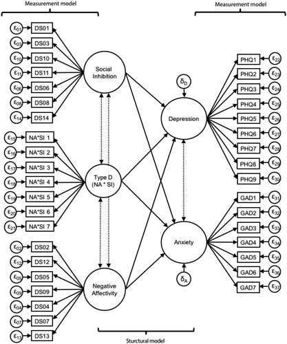
In the present study, we adopted the following terminology regarding the various aspects of latent variable models. In a latent variable model, the measurement model specifies the relation between a latent variable and a set of observed item scores intended to measure that latent variable. In the structural model, the relations between latent variables are modeled. Finally, the latent prediction model is the complete model of interest, including both the structural model and the measurement models for each latent variable. Figure 1 visualizes a latent prediction model of Type D personality, depression, and anxiety. In this figure, circles correspond to latent variables, rectangles to observed item scores, ε to the measurement error of an item, and δ to the residual error of a latent prediction effect. Dashed lines refer to covariances between latent variables and curved lines to residual covariances.

Figure 1. Latent prediction model of Type D personality, depression, and anxiety according to the matched product indicator approach. Circles correspond to latent variables; rectangles to observed variables; ε to measurement error; δ to prediction error; dashed lines to latent covariances.

To our knowledge, the relation between Type D personality, depression, and anxiety has never been investigated while taking into account measurement error and nonnormally distributed item scores. Therefore, the aim of the present study was to tackle these problems in two separate studies. In Study 1, we aimed to provide less biased estimates of the association between Type D, depression and anxiety by applying a latent prediction model to a data set of people with diabetes. In Study 2, we aimed to investigate the accuracy and stability of the estimated Type D effect in Study 1, by conducting a simulation study. Building such a latent prediction model, however, requires modeling the latent interaction. Therefore, in the next paragraph we discuss some issues related to building latent interaction models based on skewed and ordinal data.

Assessing latent variable interactions

How to handle skewed ordinal item scores?

The Type D personality, depression, and anxiety questionnaires contain items that are all measured on an ordinal scale. The item score distributions also show substantial positive skewness, as is common for clinical data (Reise & Waller, 2009). For instance, most clinical questionnaires ask people to indicate how often they experience a symptom, with response indicated on a five-point Likert scale. Especially in the general population, such questionnaires usually show an overabundance of low scores indicating that people do not frequently experience these symptoms. Positively skewed distributions pose a problem to estimation methods that assume the data to be normally distributed.

By default, most statistical packages use maximum likelihood (ML) to estimate the parameters in a latent prediction model. A standard assumption of ML estimation applied to factor analysis is that the observed item scores are continuous and normally distributed (Bollen, 1989, pp. 131–134). However, in practice, factor analysis is frequently used in conjunction with ML estimation to model ordinal questionnaire data (ten Holt, van Duijn, & Boomsma, 2010). Treating the distributions of items as normal and continuous while they are in fact skewed and ordinal can lead to underestimated standard errors of the parameter estimates and hence to more false-positive conclusions on the significance of these estimates, especially if there are five of fewer response categories (Dolan, 1994; Muthén & Kaplan, 1985; Kline, 2011; Rhemtulla, Brosseau-Liard, & Savalei, 2012). Moreover, if item response variables have an ordinal measurement level, then those items are likely not linearly associated, even when they are fairly normally distributed. Such linearity is assumed by traditional factor analytic models that are based on product-moment correlations (Flora, LaBrish, & Chalmers, 2012).

Multiple alternative methods have been proposed to handle ordinal item scores in latent variable models. For example, researchers can use item response models that do not assume that the item scores are normally distributed (Rasch, 1960; Birnbaum, 1968; Samejima, 1997). If it is important to stay within a structural equation modeling framework, then research can for instance use ML estimation with robust standard errors and a robust test statistic. This robustness may result from bootstrapping or jackknife techniques (Bollen & Stine, 1993), a Satorra-Bentler correction (Satorra & Bentler, 1988) or a sandwich estimator (Yuan & Bentler, 2000).

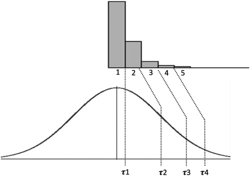
Another method that explicitly models the ordinal item scores makes use of polychoric correlations. Such correlations are estimates of the relation between two ordinal variables. This method assumes that each ordinal variable has an underlying continuous latent variable and estimates the correlation between those underlying latent variables. The two latent variables are assumed to show a bivariate normal distribution. Figure 2 illustrates the relation between such an ordinal variable and its assumed underlying continuous dimension. For each item, the boundary between each ordinal response category is connected to a latent continuous distribution through a set of threshold parameters (τ_k, where k equals the total number of response categories minus one). Each threshold marks a point on this latent indicator scale where values above and below the threshold correspond to different responses on the ordinal item. Continuous item scores between minus infinity and the value of the first threshold correspond to the lowest ordinal score. Continuous scores between the first and second threshold correspond to the second lowest ordinal score, etcetera.

Figure 2. Ordinal item score distribution (top) and the assumed underlying continuous distribution (bottom), connected by a set of polychoric threshold parameters (τ_k).

The estimated threshold parameters are subsequently combined with the information in the bivariate contingency table of two ordinal variables to estimate (using maximum likelihood) the correlation between the two underlying latent variables when they would have been observed directly (Flora & Curran, 2004). Applying this method to handle the ordinal item scores in latent prediction models first requires the matrix of polychoric correlations between all items in the model. Next, the latent prediction model is fitted to this polychoric correlation matrix. Flora and Curran (2004) suggested to use a weighted least squares (WLS) estimation procedure (Browne, 1984) to estimate the model parameters, because using ML estimation results in biased test statistics and standard errors (Babakus, Ferguson, & Jöreskog, 1987; Dolan, 1994). This WLS method uses the asymptotic variances and covariances of these polychoric correlations to estimate a weight matrix. This matrix is subsequently used in the WLS fit function to weigh the squared difference between the sample statistics and the model-implied population parameters (Muthén, 1984). Given that this method takes into account the skewness and kurtosis of the raw data, it is not necessary to specify distributional assumptions for the observed variables, making WLS an asymptotically distribution free estimator (Browne, 1984). A disadvantage of this method is that this asymptotic covariance matrix quickly gets larger as the number of observed variables increases, which can result in computational problems. Furthermore, it is well-established that WLS requires very large samples and under small sample sizes this method might produce inflated chi-square statistics (Dolan, 1994) and negatively biased standard errors (Potthast, 1993). In such a scenario, it is recommended to use unweighted least-squares (ULS) or diagonally weighted least-squares (DWLS or robust WLS) because these methods do not suffer from these limitations (Flora & Curran, 2004; Flora, LaBrish, & Chalmers, 2012).

An assumption of the polychoric correlation method is that the observed bivariate distributions between ordinal indicators can be explained from underlying bivariate normally distributed continuous variables (Olsson, 1979). This conveniently shifts the distributional assumption from the observed scores to the latent indicator level. Even then, this bivariate normality assumption is under some circumstances not necessary. Indeed, WLS estimation of a confirmatory factor analysis based on the polychoric correlation matrix is robust-to-moderate violations of this normality assumption (Flora & Curran, 2004). Furthermore, Muthén and Kaplan (1985) showed that WLS estimation in general is robust to nonnormality when sample size is larger than 1000. A final advantage of this WLS method based on polychoric correlations is that it is much more efficient than full information ML estimation, especially when modeling multiple correlated traits (Forero & Maydeu-Olivares, 2009). Given these advantages, we aim to test the fit of our latent prediction model to the polychoric correlation matrix and estimate our parameters with DWLS estimation. This method results in a less parsimonious model because it requires estimation of additional threshold parameters for each item. We will therefore also investigate whether ML estimation with the Satorra-Bentler correction for robust standard errors (MLR estimation) works equally well.

How to construct a latent interaction model?

To investigate the effect of Type D personality on depression and anxiety within a latent prediction model, one has to decide on how to extract information from the observed scores to draw inferences about the interaction between the NA and SI traits at a latent level. In methods based on sum scores, the interaction variable results from a multiplication of the two sum scores. An alternative is to multiply—rather than sum—item scores, resulting in one or more multiplied item pairs serving as indicators of a latent interaction construct.

We can test latent interaction effects according to multiple methods. When the indicant product approach is utilized, all items of the first construct are multiplied with all possible combinations of items of the second construct (Kenny & Judd, 1984). With an increasing number of items that measure each construct, this method quickly results in a very large number of indicators of the latent interaction variable. For example, both NA and SI are measured with seven items by the 14-item Type D Scale (DS14; Denollet, 2005), resulting in a total of 49 (7 multiplied by 7) additional indicators. These new indicator variables share a lot of information because they are all based on the same collection of observed variables. This large number of overlapping indicators might result in convergence problems and is computationally very demanding (Ping, 1995). The method also requires adding complex parameter constraints to the model. Therefore, it is preferable to use methods that both require a smaller number of indicator variables and that do not require complex parameter constraints.

Marsh, Wen, and Hau (2004) proposed an unconstrained method to model latent interaction effects using less indicator variables than the indicant product approach. Two examples of such unconstrained approaches are the single product indicator (Single PI) approach and the matched product indicator (Matched PI) approach. These methods differ with respect to the number of new indicators loading on the latent interaction construct. The Single PI approach uses a Single PI, while the Matched PI uses two or more new product indicators. Each indicator is the result of a multiplication of two items—one of each construct. Items sets can either be chosen at random or based on the ranking of the standardized factor loadings. For example, first the items are ranked according to their reliability based on the standardized factor loadings, and then the product of items with a similar standardized factor loading ranking is computed (Marsh, Wen, & Hau, 2004).

In a simulation study, Marsh et al. (2004) showed that the Matched PI approach results in the same amount of bias in the estimated interaction as the indicant product approach, while the Single PI approach is more biased than both other approaches. Of the two approaches with the least amount of bias, the Matched PI approach is preferable over the indicant product approach, because it is easier to implement, does not require complex constraints and is computationally less demanding.

Another way to model latent interactions is the latent moderated structural equations approach (LMS; Klein & Moosbrugger, 2000; see also Maslowsky, Jager, & Hemken, 2015). Compared to the Single PI and Matched PI approaches, LMS does not multiply item scores, nor does it model the interaction term as a latent variable. Instead, LMS directly takes into account the nonnormality of nonlinear effects by representing the joint distribution of all indicator variables as a mixture of normal distributions. Interactions are inherently nonlinear and tend to have nonnormal distributions, even when the latent variables constituting the interaction are themselves normally distributed. LMS assumes that the indicators of the exogenous latent variables conform to a multivariate normal distribution. Given the nonnormally distributed item scores of the Type D questionnaire, we expect in line with earlier research (Kelava & Nagengast, 2012; Kelava, Nagengast, & Brandt, 2014), that the LMS approach shows bias in the estimation of the latent interaction. Furthermore, we expect the Single PI and Matched PI approach to show less bias than the LMS method because earlier research showed that these approaches, especially the Matched PI approach, were less biased than LMS when the data are not normally distributed (Marsh et al., 2004; Cham, West, Ma, & Aiken, 2012).

Study overview

In Study 1, we used a latent prediction model to investigate the association of Type D personality with depression and anxiety. Type D personality was modeled as an interaction between its components negative affectivity and social inhibition (Smith, 2011). All constructs are positively skewed and measured with multiple items measured on an ordinal scale. Given that earlier simulation studies on latent interaction modeling did not investigate the performance of the Single PI, Matched PI and LMS approaches under these specific circumstances, we applied all three approaches and compared their performance in a simulation study. Therefore, in Study 2, we performed a Monte Carlo simulation to investigate to what extent the models used in Study 1 provided accurate and stable parameter estimates given the specific characteristics of Study 1 (i.e., large sample size, large positive skewness, and ordinal item scores).

Study 1: Latent prediction model in adults with diabetes

Method

Participants

Data were used from the Diabetes MILES study (Nefs, Bot, Browne, Speight, & Pouwer, 2012), containing a sample of 3314 Dutch adults with type 1 or 2 diabetes. The psychological research ethics committee of Tilburg University approved of the study protocol (EC-2011-5). All participants gave informed consent.

Measures

DS14. The traits underlying Type D personality (NA and SI) were measured using the DS14 questionnaire (Denollet, 2005). Each trait was measured with a scale consisting of seven questions with five ordinal response categories ranging from “false” (0) to “true” (4). The DS14 has been validated in several populations (Denollet, 2005). In our sample, the coefficient alpha of NA and SI were 0.89 and 0.90, respectively.

PHQ-9. Depressive symptoms were measured using the nine-item Patient Health Questionnaire (PHQ-9; Kroenke, Spitzer, & Williams, 2001), with each item having four ordinal response categories ranging from “not at all” (0) to “nearly every day” (3). The PHQ-9 has been validated in both the general- and the diabetes population (Martin, Rief, Klaiberg, & Braehler, 2006; van Steenbergen-Weijenburg et al., 2010). In our sample, the coefficient alpha of the PHQ-9 was 0.86.

GAD-7. Anxiety symptoms were measured using the seven-item General Anxiety Disorder questionnaire (GAD-7; Spitzer, Kroenke, Williams, & Löwe, 2006), with each item having four ordinal response categories, ranging from “not at all” (0) to “nearly every day” (3). The GAD-7 has been validated in the general population (Löwe et al., 2008). In our sample, the coefficient alpha of the GAD-7 was 0.90. The item correlation matrices and skewness and kurtosis estimates are reported in Appendix A (DS14) and Appendix B (PHQ-9 and GAD-7).

Software

We performed all analyses in the freely available R programing software (version 3.2.3; R development Core Team, 2008) and used Mplus software (version 8; Muthén & Muthén, 1998, 2010) to build our latent interaction models. The Mplus syntax files are available at this project’s open science framework page: https://osf.io/kf6d5/.

Model building

To identify our model, we fixed the first factor loading of each latent trait to a value of one. The latent prediction model was built in several steps. We first created separate measurement models for Type D personality, depression, and anxiety. These measurement models were then used to evaluate whether the data fitted a predetermined factor structure. Both the depression and anxiety questionnaires should exhibit a one-factor structure (Kroenke, Spitzer, & Williams, 2001; Spitzer et al., 2006), whereas the Type D questionnaire should show a two-factor structure.

In the next step, we connected these measurement models by including a structural model. We took a multivariate approach by first regressing depression and anxiety on both NA and SI, thereby investigating the main effects of Type D on depression and anxiety. Subsequently, we added the latent interaction between NA and SI, thereby testing whether the interaction between NA and SI explains any additional variance in depression or anxiety above and beyond the variance explained by the additive effects of NA and SI.

Our model selection procedure involved the comparison of three nested models. The first model is a baseline model where all regressions between latent constructs were fixed to zero. This model served as a reference model against which we compared the fit of our second model. In Model 2, we estimated the main effects of NA and SI on both depression and anxiety. Finally, in Model 3 we included the interaction between NA and SI on both depression and anxiety. Lastly, we tested the quadratic effects of both NA and SI to determine whether a possible interaction effect was merely picking up an unmodeled quadratic effect rather than a true interaction (MacCallum & Mar, 1995).

Interaction models

We assessed the interaction between NA and SI according to six different methods: (1) Regression of sum scores, (2) LMS using robust maximum likelihood (MLR) estimation, (3) Matched PI using MLR estimation, (4) Single PI using MLR estimation, (5) Matched PI based on the polychoric correlation matrix using diagonally weighted least squares (DWLS) estimation, and (6) Single PI based on the polychoric correlation matrix using DWLS estimation. For the matched and Single PI approaches, the pairing of the NA and SI indicators (constituting the latent interaction term) was based on the ranking of the estimated standardized factor loadings of the Type D measurement model. For the Matched PI approach, we used seven indicator pairs and for the Single PI approach one indicator pair.

Model fit

Model fit was assessed by inspecting the $\chi$² test, the Bayesian Information Criterion (BIC; Schwarz, 1978), as well as the Comparative Fit Index (CFI), the Tucker-Lewis Index (TLI), and Root Mean Square Error of Approximation (RMSEA). For both the TLI and CFI, we assumed values above 0.95 to indicate adequate fit (Hu & Bentler, 1999). For the RMSEA, we considered values above 0.10 as unacceptable and values below 0.06 as indicating good model fit (Chen et al., 2008). For some of the investigated methods, not all of these fit indices were available.¹ In these situations, all available fit indices were reported. Nested models were compared using a chi-square or log-likelihood difference test, depending on the type of interaction model. For the PI MLR methods, we used the Satorra and Bentler (2010) scaled χ² difference between two models against their difference in degrees of freedom (df). For the PI DWLS, we used the T3 test (Asparouhov & Muthén, 2010), a nested model comparison test developed specifically for ordinal nonnormal data. Lastly, for the LMS method, we used the chi-square difference test based on log likelihood values and scaling correction factors obtained with MLR estimation.

Results

Of all 3314 participants, 3 (0.1%) did not complete the PHQ-9 questionnaire and 9 (0.27%) did not complete the GAD-7 questionnaire. We excluded these participants from our latent prediction model. Tables 1–3 show the fit statistics and parameter estimates for several tested models according to the six different ways to model the interaction effect between NA and SI on depression and anxiety. Table 1 focuses on the Sum score approach, while Tables 2 and 3 focus on the latent variable approaches.

Table 1. Association between Type D personality, depression, and anxiety using linear hierarchical regression analyses.

Dependent measure	Model	Model fit (F-test)	Nested model difference test (ΔF)	NA		SI		SI × NA		NA^2		SI^2
				B (SE)	β	B (SE)	β	B (SE)	β	B (SE)	β	B (SE)	β
Depression	1	F(2,3308) = 1346.0*	–	3.08 (.07)*	.66	.06 (.07)	.01	–	–	–	–	–	–
	2a	F(3,3307) = 955.3*	F(1,3307) = 96.2*	3.02 (.07)*	.68	.003 (.07)	.001	.56 (.06)*	.13	–	–	–	–
	2b	F(4,3306) = 802.4*	F(1,3306) = 143.0*	2.69 (.07)*	.70	.03 (.07)	.01	–	–	.79 (.05)*	.21	.21 (.05)*	.06
	3	F(5,3305) = 641.9*	F(1,3305) = .46	2.69 (.07)*	.69	.03 (.07)	.01	.05 (.07)	.01	.78 (.06)*	.20	.19 (.06)*	.05
Anxiety	1	F(2,3302) = 1561.0*	–	2.64 (.05)*	.72	–.18 (.05)*	–.05	–	–	–	–	–	–
	2a	F(3,3301) = 1077.0*	F(1,3301) = 56.0*	2.60 (.05)*	.74	–.21 (.05)	–.06	.33 (.04)*	.09	–	–	–	–
	2b	F(4,3300) = 902.7*	F(1,3300) = 125.9*	2.33 (.05)*	.77	–.17 (.05)*	–.06	–	–	.60 (.04)*	.20	.08 (.04)*	.03
	3	F(5,3299) = 722.3*	F(1,3299) = .90	2.34 (.05)*	.75	–.17 (.05)*	–.05	–.05 (.05)	–.02	.62 (.05)*	.20	.10 (.05)*	.03

Model 1: NA and SI main effects.

Model 2a: NA and SI main + interaction effects.

Model 2b: NA and SI main + quadratic effects.

Model 3: NA and SI main + quadratic + interaction effects.

β = standardized regression coefficient; B = unstandardized regression coefficient.

*p<.05.

Table 2. Model fit indices and structural regression coefficients for each of the five methods to model latent interactions.

Method	Model	Parameters (df)	Model fit indices						Latent regression effects on depression					Latent regression effects on anxiety
			χ^2 or LL	χ^2 or LL difference test (df)^a	BIC	RMSEA (95% CI)	CFI	TLI		SI	NA	SI × NA	$\beta$		SI	NA	SI × NA	$\beta$
Single PI MLR	1	96 (400)	6915.1*	–	216231.9	.067 [ .066 .069 ]	0.843	0.831		–	–	–	–		–	–	–	–
	2	100 (396)	4935.6*	2437.6 (4)*	213474.9	.057 [.055 .058]	0.891	0.881		–.05 (.01)*	.74 (.04)*	–	–		−.08 (.01)*	.73 (.03)*	–	–
	3	102 (394)	4852.3*	61.0(2)*	213353.8	.056 [.055 .058]	0.893	0.883		−.05 (.01)*	.66 (.04)*	.13 (.02)*	0.24		–.09 (.01)*	.67 (.03)*	.09 (.02)*	0.16
Single PI DWLS	1	140 (356)	59500.9*	–	NA^b	.204 [ .202 .205 ]	0.584	0.551		–	–	–	–		–	–	–	–
	2	144 (352)	7983.4*	6376.5 (4)*	NA^b	.073 [.072 .075]	0.947	0.942		−.11 (.02)*	1.37 (.04)*	–	–		–.20 (.02)*	1.49 (.04)*	–	–
	3	146 (350)	7831.4*	144.7 (2)*	NA^b	.073 [.071 .074]	0.948	0.943		−.12 (.02)*	1.28 (.04)*	.14 (.01)*	0.16		–.20 (.02)*	1.43 (.04)*	.09 (.01)*	0.11
Matched PI MLR	1	115 (588)	7464.9*	–	282889.9	.058 [.056, .059]	0.844	0.833		–	–	–	–		–	–	–	–
	2	119 (584)	5549.2*	2479.6 (4)*	280149.3	.049 [.048 .050]	0.887	0.879		−.04 (.01)*	.74 (.04)*	–	–		–.08 (.01)*	.72 (.03)*	–	–
	3	121 (582)	5479.3*	111.6 (2)*	280053.3	.049 [.048 .050]	0.889	0.880		−.05 (.01)*	.70 (.04)*	.09 (.01)*	0.16		–.09 (.01)*	.71 (.03)*	.05 (.01)*	0.09
Matched PI DWLS	1	159 (544)	60679.9*	–	NA^b	.171 [.169 .172]	0.602	0.576		–	–	–	–		–	–	–	–
	2	163 (540)	8410.1*	6209.4 (4)*	NA^b	.062 [.060 .063]	0.948	0.945		–.12 (.02)*	1.41 (.04)*	–	–		–.21 (.02)*	1.51 (.04)*	–	–
	3	165 (538)	8164.7*	156.1 (2)*	NA^b	.061 [.060 .062]	0.950	0.946		−.12 (.02)*	1.32 (.04)*	.10 (.01)*	0.13		–.20 (.02)*	1.46 (.04)*	.06 (.01)*	0.07
LMS MLR	1	92 (373)	−101940.5	–	204626.5	NA^c	NA^c	NA^c		–	–	–	–		–	–	–	–
	2	96 (369)	−100563.7	2553.6 (4)*	201905.3	NA^c	NA^c	NA^c		−.04 (.01)*	.76 (.04)*	–	–		–.08 (.01)*	.75 (.03)*	–	–
	3	98 (367)	−100445.3	88.4(2)*	201684.7	NA^c	NA^c	NA^c		−.04 (.01)*	.69 (.04)*	.21 (.02)*	0.21		–.08 (.01)*	.70 (.03)*	.13 (.02)*	0.14

In Model 1, the NA and SI main- and interaction effects are fixed to zero. In Model 2, only the interaction effects are fixed to zero. In Model 3, all structural regression coefficients are freely estimated.

Numbers printed in bold indicate better fit of one model relative to the other. Latent regression effects are reported in terms of unstandardized regression coefficients and their corresponding standard errors.

β denotes the standardized regression coefficient of the latent interaction effect.

*p<.001.

^aThis column shows for the PI MLR methods the Satorra & Bentler (2010) scaled χ² difference between two models against their difference in degrees of freedom (df). For the PI DWLS methods, the column shows the T3 test (Asparouhov & Muthén, 2010), a nested model comparison test developed specifically for ordinal nonnormal data. For the LMS method, this column shows the likelihood ratio test based on log likelihood values and scaling correction factors obtained with MLR estimation.

^bAs the BIC is based on the log likelihood which is not computed in the DWLS methods, Mplus does not report this fit index for models involving weighted least squares estimation.

^cWhen numerical integration is required (e.g., with the LMS method), means, variances, and covariances are not sufficient statistics for model estimation and chi-square and related fit statistics are not available. Therefore, Mplus does for report the chi-square statistics and related indices (RMSEA, CFI, TLI) for the LMS method.

Table 3. Model fit indices and structural regression coefficients for each of the five methods to model latent interactions and quadratic effects.

Method	Model	Parameters (df)	Model fit indices						Latent regression effects on depression					Latent regression effects on anxiety
			χ^2 or LL	χ^2 or LL difference test (df)^a	BIC	RMSEA (95% CI)	CFI	TLI		SI^2	NA^2	SI × NA	$\beta$		SI^2	NA^2	SI × NA	$\beta$
Single PI MLR	1	115 (381)	5401.8*	–	237,632.6	.056 [.054 .057]	0.886	0.874		.35 (.11)*	−.07 (.06)	–	–		.22 (.07)*	0 (.04)	–	–
	2	117 (379)	5390.9*	12.32 (2)*	237,629.7	.056 [.055 .057]	0.886	0.874		.09 (.05)	.01 (.02)	.10 (.03)*	0.19		.07 (.04)	.04 (.02)*	.05 (.02)*	0.10
Single PI DWLS	1	159 (337)	9334.1*	–	NA^b	.075 [.073 .076]	0.947	0.942		−.29 (.06)*	.22 (.02)*	–	–		−.30 (.06)*	.22 (.02)*	–	–
	2	161 (335)	9225.5*	128.8 (2)*	NA^b	.075 [.073 .076]	0.948	0.942		−.23 (.05)*	.10 (.02)*	.18 (.02)*	0.21		−.30 (.05)*	.15 (.03)*	.14 (.02)*	0.16
Matched PI MLR	1	172 (531)	15,356.2*	–	437,610.0	.060 [.059 .060]	0.780	0.767		.04 (.02)*	.35 (.06)*	–	–		.05 (.02)*	.19 (.05)*	–	–
	2	174 (529)	15,362.4*	2.64 (2)	437,621.5	.060 [.059 .061]	0.780	0.767		.04 (.02)*	.35 (.06)*	.00 (.02)	0.00		.06 (.02)*	.22 (.05)*	−.02 (.02)	−0.04
Matched PI DWLS	1	230 (473)	18,482.5*	–	NA^b	.093 [.092 .094]	0.738	0.723		2.54 (1.50)	−1.54 (.86)	–	–		3.64 (2.12)	−2.06 (1.21)	–	–
	2	232 (471)	18,477.7*	38.0 (2)*	NA^b	.093 [.092 .094]	0.738	0.723		.45 (.18)*	−.32 (.10)*	−.02(.01)	−0.05		.42 (.27)*	−.18 (.14)*	−.04 (.02)*	−0.07
LMS MLR	1	100 (365)	−100,012.1	–	200,834.4	NA^c	NA^c	NA^c		0 (.01)	.49 (.04)*	–	–		−.02 (.01)*	.42 (.04)*	–	–
	2	102 (363)	−100,201.0	12.55 (2)*	201,228.4	NA^c	NA^c	NA^c		.05(.02)*	.22 (.01)*	−.09 (.03)*	−0.15		.04 (.01)*	.20 (.01)*	−.11 (.03)*	−0.19

Model 1 estimates the NA and SI main and quadratic effects, while Model 2 additionally includes their interaction effects.

Numbers printed in bold indicate better fit of one model relative to the other. Latent regression effects are reported in terms of unstandardized regression coefficients and their corresponding standard errors.

β denotes the standardized regression coefficient of the latent interaction effect.

*p<.05.

^aThis column shows for the PI MLR methods the Satorra & Bentler (2010) scaled χ² difference between two models against their difference in degrees of freedom (df). For the PI DWLS methods, the column shows the T3 test (Asparouhov & Muthén, 2010), a nested model comparison test developed specifically for ordinal nonnormal data. For the LMS method, this column shows Wald test on the parameter constraints that the estimates of the interaction effect on both depression and anxiety are equal to zero.

^bAs the BIC is based on the log likelihood which is not computed in the DWLS methods, Mplus does not report this fit index for models involving weighted least squares estimation.

^cWhen numerical integration is required (e.g., with the LMS method), means, variances, and covariances are not sufficient statistics for model estimation and chi-square and related fit statistics are not available. Therefore, Mplus does for report the chi-square statistics and related indices (RMSEA, CFI, TLI) for the LMS method.

Sum score approach

According to the Sum score approach, the models including the interaction between NA and SI fitted the data better than the models without the interaction term. There was a significant interaction between NA and SI on both depression [b = 0.561, t(3308) = 9.807, p < .001, β = 0.126] and anxiety [b = 0.329, t(3302) = 7.481, p < .001, β = 0.093]. However, first including the NA and SI quadratic resulted in significant quadratic effects and rendered the interaction between the two constructs nonsignificant, both with respect to depression [b = 0.048, t(3308) = 0.678, p = .498, β = 0.012] and anxiety [b = −0.052, t(3302) = −0.95, p=.342, β = −0.017]. Moreover, the model including the interaction term did not significantly explain additional variance in both depression and anxiety, above and beyond the NA and SI main and quadratic effects. This suggests that the Type D effect might be confounded by quadratic NA and SI effects.

Single PI (MLR) approach

Table 2 shows that for the Single PI approach with MLR estimation, all three nested models resulted in a significant $\chi$² value, indicating that the model-implied covariance matrix deviated from the observed covariance matrix, a sign of poor exact model fit. The BIC favored the model including the interaction between NA and SI (Model 3) above the model without interaction effects (Model 3). The RMSEA suggested that both Models 2 and 3 showed good fit, because the upper bound of the 95% confidence interval was below 0.06. According to the CFI and TLI, none of the models showed acceptable fit, although the model including interaction effects showed better fit than the other two models.

The chi-square difference tests indicated an improved fit of a model over its predecessor. Of particular interest is the significant difference in fit between Models 2 and 3, indicating that the model including the interaction effect significantly explained additional variation in anxiety and depression scores above and beyond the model with the NA and SI main effects only. The Single PI MLR approach showed significant regression coefficients for the interaction between NA and SI for both depression (b = 0.13, z = 6.29, p < .001, β = 0.24) and anxiety (b = 0.09, z = 4.70, p < .001, β = 0.16).

To investigate whether the interaction effect merely reflected unmodeled quadratic effect, Table 3 shows the comparison of a model including the NA and SI main- and quadratic effects with a model also including the interaction effect. As the RMSEA, CFI and TLI almost always resulted in similar fit measures for both models, we decided to only report these results in Table 3. It turned out that based on the BIC and chi-square differences test, the model including main, quadratic and interaction effect fitted the data significantly better than the model with main and quadratic effects only, suggesting that the interaction effect did not merely reflect quadratic NA and SI effects. After including the quadratic effects, the estimated interaction effects remained statistically significant for both depression (b = 0.10, z = 4.01, p < .001, β = 0.19) and anxiety (b = 0.05, z = 2.35, p = .019, β = 0.10).

Single PI (DWLS) approach

Table 2 shows the results for the Single PI approach with WLS estimation based on the polychoric correlation matrix. Again, all three nested models resulted in a significant $\chi$² value, a sign of poor exact model fit. The RMSEA suggested that both Models 2 and 3 showed reasonable fit with the upper bound of the 95% confidence interval below 0.08. For both models 2 and 3, the CFI and TLI were just below 0.95, suggesting good fit.

The two nested model comparison tests indicated an improved fit of Model 2 over Model 1 and of Model 3 over Model 2, suggesting that both the NA and SI main effects, as well as their interaction is of added value to the model. The Single PI DWLS approach showed significant regression coefficients for the interaction between NA and SI for both depression (b = 0.14, z = 11.34, p<.001, β = 0.16) and anxiety (b = 0.09, z = 7.21, p<.001, β = 0.11).

Table 3 shows that based on the nested model comparison test, the model including main, quadratic and interaction effects fitted the data significantly better than the model including main and quadratic effects only. After including the quadratic effects, the estimated interaction effects remain statistically significant for both depression (b = 0.18, z = 10.07, p<.001, β = 0.21) and anxiety (b = 0.14, z = 6.77, p<.001, β = 0.16).

Matched PI (MLR) approach

Table 2 shows the results of the Matched PI approach with MLR estimation. All three models resulted in a significant $\chi$² value, a sign of poor exact model fit. However, the BIC favored the model with the interactions (Model 3) above the model without the interactions (Model 2). According to the RMSEA, CFI and TLI, the model including the interactions fitted the data best. The RMSEA of both Model 2 and 3 showed an upper bound of the 95% confidence interval of 0.05. According to both the CFI and TLI, all models showed suboptimal fit with values of approximately 0.88.

The chi-square difference tests indicated an improved fit of a model over its predecessor. Hence, including the interactions (Model 3) resulted in significantly better fit than fixing the interactions to zero (Model 2). The estimated regression coefficients in Model 3 showed a significant interaction between NA and SI for both depression (b = 0.09, z = 7.77, p<.001, β = 0.16) and anxiety (b = 0.05, z = 4.59, p<.001, β = 0.09).

Table 3 shows that based on the BIC and the nested model comparison test, the model including main, quadratic and interaction effects did not significantly fit the data better than the model including main and quadratic effects only. After including the quadratic effects, the estimated interaction effects did no longer reach statistical significance for both depression (b = 0.00, z = −0.14, p = .892, β = 0.00) and anxiety (b = −0.02, z = −1.40, p = .163, β = −0.04).

Matched PI (DWLS) approach

Table 2 shows the results of the Matched PI approach with DWLS estimation based on the polychoric correlation matrix. All three models resulted in a significant $\chi$² value, a sign of poor exact model fit. According to the RMSEA, CFI and TLI, the model including the interactions fitted the data best. Both Models 2 and 3 showed RMSEA 95% confidence intervals around 0.06. According to both the CFI and TLI, Models 2 and 3 showed good fit with values of approximately 0.95.

The nested model comparison tests indicated an improved fit of a model over its predecessor. Hence, including the interactions (Model 3) resulted in significantly better fit than fixing the interactions to zero (Model 2). The estimated regression coefficients in Model 3 showed a significant interaction between NA and SI for both depression (b = 0.10, z = 12.00, p<.001, β=.13) and anxiety (b=.06, z = 6.95, p<.001, β=.07).

Table 3 shows that based on the nested model comparison test, the model including main, quadratic and interaction effects fitted the data significantly better than the model including main and quadratic effects only. After including the quadratic effects, the estimated interaction effect no longer reached statistical significance for depression (b= −0.02, z= −1.53, p = .126, β= −0.05) yet remained significant for anxiety (b= −0.04, z= −2.17, p=.03, β= −0.07).

LMS approach

Table 2 shows the results of the LMS approach using MLR estimation. According to the BIC, the model with the interaction term (Model 3) fitted the data better than the model without the interaction term (Model 2) for both outcome variables. The likelihood ratio test too indicated that inclusion of the interaction terms resulted in a significantly improvement in model fit. Model 3 showed a significant interaction between NA and SI for both depression (b = 0.21, z = 8.93, p<.001, β = 0.21) and anxiety (b = 0.13, z = 6.02, p<.001, β = 0.14). Table 3 shows that based on the nested model comparison test, the model including main, quadratic and interaction effects fitted the data significantly better than the model including main and quadratic effects only [Wald(2)=12.55, p=.002).² After including the quadratic effects, the estimated interaction effects remained statistically significant, but switched signs both for depression (b= −0.09, z= −2.7, p = .007, β= −0.15) and anxiety (b= −0.11, z= −3.54, p<.001, β= −0.19).

Factor scores

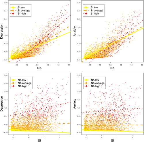
Figure 3 shows in four separate plots for both NA and SI the association with depression and anxiety. Each plot shows the effect of NA or SI for three different levels of the other construct (low< −1 SD < average< +1 SD < high). All axes show factor scores estimated with the Maximum A Priori method in Mplus. Visual inspection of these plots suggest two competing interpretations: either the effects of NA or SI on depression and anxiety get stronger at higher levels of the other construct, or NA and SI show quadratic effects on depression and anxiety, where the association gets stronger at higher levels of each construct. The estimated factor scores show good factor indeterminacy values (NA = 0.964; SI = 0.952; Depression = 0.959; Anxiety = 0.965).

Figure 3. Plots showing the association between NA and depression (upper left), between NA and anxiety (upper right), between SI and depression (lower left), and between SI and anxiety (lower right). Each plot shows the effect of NA or SI for three different levels of the other construct (low< −1 SD < average< +1 SD < high). All axes show factor scores estimated with the Maximum A Priori method in Mplus.

Summary

To summarize, according to all six methods, the interaction between NA and SI was significantly associated with both depression and anxiety, although the size of this interaction varied across the tested methods. Moreover, when first adding the quadratic effects to the model, all methods produced smaller estimates of the interaction effects. For both Single PI methods, the interaction effects remained significant, while for other methods the interaction reduced to zero (Sum score; Matched PI MLR; Matched PI DWLS), or even changed the effect in the opposite direction (LMS). Because the estimates of both the quadratic and interaction effects vary not only across the method used to model the nonlinear effects, but also across the estimation method (e.g., MLR versus DWLS), we doubt the robustness of the models including both quadratic and interaction terms and we advise readers to interpret the results of these models with care. Given these conflicting results, we need additional evidence to support the robustness of the findings in Study 1. Therefore, in Study 2, we conducted a simulation to compare these six methods to model interactions on the bias and precision of the estimated interaction effect.

Study 2: Simulation study

Method

Procedure

In our simulation study, we varied four different design parameters: scale (continuous, ordinal), item skewness (0, 2 and 3), the size of the interaction (0, .10, .20 and .40) and sample size (250, 500 and 3000). All possible combinations of these four design parameters resulted in a factorial design with 2 × 3×4 × 3=72 conditions. The anxiety (GAD-7) and depression (PHQ-9) questionnaires showed similar psychometric properties. For reasons of clarity, we decided to focus our simulation on estimating the interaction effect of NA and SI on depression.

Design Parameter 1: Scale Level. The first design parameter was the scale level of the simulated DS14 and PHQ-9 items. We either simulated continuous or ordinal item scores. For ordinal scores, the number of response categories depended on the type of questionnaire (PHQ-9 = 0–3 Likert scale; DS14 = 0–4 Likert scale).

Design Parameter 2: Skewness. The second design parameter was the amount of skewness in the distribution of the latent traits NA and SI. We used the method of Vale and Maurelli (1983) as implemented in the R-package fungible (version 1.5; Waller, 2016), to simulate a multivariate distribution of NA and SI. We varied across three skewness values (0, 2 and 3; with corresponding kurtosis values 0, 7 and 21), while retaining the product moment correlation between NA and SI (Study 1 estimate of .553),

Design Parameter 3: Size of Interaction. The third design parameter indicated the strength of the interaction between NA and SI on depression. We based the true size of the interaction on the standardized regression coefficient of the estimated interaction effect in Study 1 according to the LMS approach (β = 0.20). In our simulation, we allowed the interaction to be either absent (0), half the size of the Study 1 interaction (0.10), the exact size of the Study 1 interaction (0.20), or twice the size of the Study 1 interaction (0.40).

Design Parameter 4: Sample size. The fourth design parameter indicated the sample size of the simulated data set. We varied between a small, medium and large sample size condition. In the large sample condition, we used a sample size of 3000 participants, resembling the sample size of the data set used in Study 1. In the medium sample condition we simulated data for 500 participants, representing sample sizes commonly encountered when analyzing latent variable models. Lastly, in the small sample condition we simulated a sample size of 250 participants.

Data simulation

For each of the 72 conditions, we simulated 500 data sets containing scores on items measuring the constructs depression (9 items), NA (7 items) and SI (7 items). We generated data using the parameter estimates (i.e., factor loadings, latent (co)variances, regression coefficients, thresholds and error variances) of the latent prediction model in Study 1.³ First, we randomly sampled vectors of NA and SI latent trait scores according to the multivariate skew distribution, given the NA and SI (co)variance(s) from Study 1 and given the skewness design parameter. Second, we used Equation (1)(1) $$Y_{ij}={\mathrm{\lambda }}_{jt}{\text{ η}}_{ti}+{\mathrm{\epsilon }}_{ij}$$(1) to calculate the continuous item scores for each individual (i) and for each item (j) measuring the traits (t) NA or SI: (1) $$Y_{ij}={\mathrm{\lambda }}_{jt}{\text{ η}}_{ti}+{\mathrm{\epsilon }}_{ij}$$(1)

In this equation, ${\mathrm{\lambda }}_{jt}$ denotes the factor loading of item j loading on trait t. ${\mathrm{\eta }}_{ti}$ represents the score of individual i on latent trait t, and ${\mathrm{\epsilon }}_{ij}$ the residual error of individual i on item j. When generating the continuous item scores, we used as input a matrix with individual NA and SI trait scores ($\mathbf{\Psi }$), the factor loading matrix retrieved from Study 1 ($\mathbf{\Lambda }$), and a residual error matrix ($\mathbf{\Theta }$) based on a multivariate normal distribution with a mean vector of zeroes and a diagonal covariance matrix with variances retrieved from the output in Study 1. In line with earlier research (Flora & Curran, 2004), for ordinal scenarios, we transformed these continuous item scores into ordinal scores using the case 1 thresholds proposed by Muthén and Kaplan (1985).

To simulate PHQ-9 (depression) item scores, we had to take into account that the scores on the depression measure depended on the scores of the NA and SI traits, their interaction, and prediction error. Therefore, we used Equation (2)(2) $${\psi }_{Di}={\beta }_{SI}{\psi }_{SIi}+{\beta }_{NA}{\psi }_{NAi}+{\beta }_{NA\mathrm{*}SI}{\psi }_{NAi}{\psi }_{SIi}+{\delta }_i$$(2) to first compute the latent depression scores: (2) $${\psi }_{Di}={\beta }_{SI}{\psi }_{SIi}+{\beta }_{NA}{\psi }_{NAi}+{\beta }_{NA\mathrm{*}SI}{\psi }_{NAi}{\psi }_{SIi}+{\delta }_i$$(2)

We then used Equation (1)(1) $$Y_{ij}={\mathrm{\lambda }}_{jt}{\text{ η}}_{ti}+{\mathrm{\epsilon }}_{ij}$$(1) to compute the continuous depression item scores and if appropriate we used the case 1 thresholds (Muthén & Kaplan, 1985) to transform them into ordinal item scores. In Equation (2)(2) $${\psi }_{Di}={\beta }_{SI}{\psi }_{SIi}+{\beta }_{NA}{\psi }_{NAi}+{\beta }_{NA\mathrm{*}SI}{\psi }_{NAi}{\psi }_{SIi}+{\delta }_i$$(2) , ${\psi }_{Di}$ denotes the latent depression score of individual i, the three ${\beta }^{\prime }s$ represent the regression coefficients of the latent regression of depression on NA (${\psi }_{NAi}$), SI (${\psi }_{SIi}$) and the interaction between NA and SI (${\psi }_{NAi}*{\psi }_{SIi}$). Lastly, ${\delta }_i$ denotes the prediction residual of individual i, based on normal distribution with mean zero and a variance retrieved from the output of Study 1.

Statistical methods

After simulating 500 data sets in each of the 72 conditions, we analyzed each data set according to the same methods used in Study 1: (1) Regression of sum scores; (2) LMS with MLR estimation; (3) Single PI with MLR estimation; (4) Matched PI with MLR estimation; (5) Single PI with DWLS estimation based on the polychoric correlation matrix; and (6) Matched PI with DWLS estimation based on the polychoric correlation matrix. Note that we only applied methods 5 and 6 to data sets with ordinal item scores, because the polychoric thresholds could not be estimated for data with continuous measurement levels. We implemented all latent interaction models in Mplus and conducted the simulation using the R-package MplusAutomation (Hallquist & Wiley, 2011). The R-script of this simulation study is available at this project’s open science framework page: https://osf.io/kf6d5/.

Outcome measures

We aggregated the parameter estimates over 500 replications and used the mean and standard deviation to compute a 95% confidence interval for the parameters of interest. Our main outcome was the bias and precision of the parameter estimates. The amount of bias was computed as the difference between the mean of a parameter estimate and the true value (i.e., the $\beta$ values of used to generate the data; see Equation (2)(2) $${\psi }_{Di}={\beta }_{SI}{\psi }_{SIi}+{\beta }_{NA}{\psi }_{NAi}+{\beta }_{NA\mathrm{*}SI}{\psi }_{NAi}{\psi }_{SIi}+{\delta }_i$$(2) ). We also assessed the mean squared error, defined as the squared distance between the estimated value of the interaction effect and the true value of the interaction, averaged across 500 replications. We used the width of the 95% confidence interval as a measure of precision in the parameter estimate.

Expectations

With respect to simulation conditions with continuous item scores, we expected in line with earlier research (Kelava & Nagengast, 2012; Kelava, Nagengast, & Brandt, 2014), that LMS would perform best when the latent traits are normally distributed and that it would get more biased as skewness increased. Furthermore, we expected the PI approaches to show less bias in skewed conditions than the LMS method because earlier research showed that these approaches, especially the Matched PI approach, were less biased than LMS when the data is not normally distributed (Marsh et al., 2004; Cham, West, Ma, & Aiken, 2012). With respect to simulation conditions with ordinal item scores, we expected the WLS approach that used the polychoric correlation matrix to outperform the MLR approach based on the product moment correlation matrix, because the former method directly models skewness by estimating threshold parameters for each item. Finally, we expected the Sum score approach to underestimate the interaction effects because the presence of measurement error attenuates the true association between the latent constructs.

Results

All methods except LMS showed a 100% convergence rate. In conditions without skewness, LMS also reached 100% convergence, but as skewness increased the convergence rate decreased to approximately 90% for N = 500, and 85% for N = 250 conditions. Nonconverged solutions have been excluded from further analyses.

For all 72 conditions in our stimulation study, Appendices C and D show respectively for continuous and ordinal item score conditions the mean parameter estimates of the interaction (including 95% confidence interval). Appendix E presents for all simulation conditions the bias in the estimated interaction effect in terms of the squared distance between the estimated interaction and the true interaction, averaged across all 500 replications (mean squared error). Table 4 summarizes these statistics by reporting the total mean squared error for each level of every design factor used in our simulation study. Lastly, Table 5 shows for each scenario the percentage of significant interaction effects across all 500 replications, given a significance level of 0.05.

Table 4. For all methods, the total mean squared error across conditions involving specific design factors.

Design factor	Continuous item scores				Ordinal item scores
							Single PI		Matched PI
	Sum score regression	LMS MLR	Single PI MLR	Matched PI MLR	Sum score regression	LMS MLR	MLR	DWLS	MLR	DWLS
All simulation conditions	0.145	0.058	5.723	0.291	0.110	0.085	0.530	0.494	0.117	0.116
N = 250	0.059	0.028	2.018	0.107	0.048	0.041	0.185	0.175	0.059	0.057
N = 500	0.048	0.019	2.261	0.095	0.036	0.028	0.176	0.164	0.037	0.037
N = 3000	0.039	0.012	1.445	0.089	0.026	0.017	0.169	0.155	0.021	0.021
Skewness = 0	0.012	0.012	0.022	0.045	0.014	0.013	0.083	0.090	0.038	0.031
Skewness = 2	0.043	0.023	0.881	0.083	0.044	0.034	0.206	0.186	0.036	0.040
Skewness = 3	0.091	0.023	4.820	0.163	0.052	0.038	0.241	0.219	0.043	0.045
β = 0	0.011	0.008	0.114	0.013	0.018	0.021	0.007	0.008	0.019	0.022
β = .1035	0.032	0.015	0.972	0.050	0.019	0.023	0.016	0.015	0.029	0.033
β = .207	0.057	0.023	2.095	0.109	0.010	0.016	0.073	0.067	0.029	0.030
β = .414	0.045	0.012	2.542	0.119	0.064	0.026	0.434	0.405	0.040	0.030

β denotes the standardized regression coefficient of the true interaction effect.

Table 5. For each simulation condition, the percentage of statistically significant (p < .05) interaction effects.

			Continuous item scores				Ordinal item scores
		True size	Sum score	LMS	Single	Matched	Sum score	LMS	Single PI		Matched PI
N	Skewness	interaction	regression	MLR	PL MLR	PI MLR	regression	MLR	MLR	DWLS	MLR	DWLS
250	0	0	7.6	8.4	5.4	8.2	6.4	5.8	5.4	13.0	5.6	12.8
		.1035	81.6	86.8	67.4	82.6	75.4	82.0	50.2	69.2	75.0	86.0
		.207	100	100	98	100	100	100	94.8	98.0	100	100
		.414	100	100	100	100	100	100	100	100	100	100
	2	0	7.0	7.04	2.2	4.4	13.4	15	4.0	15.4	7.0	21.8
		.1035	93.4	94.5	28.8	85.0	89	92.4	46.8	71.8	69.2	91.8
		.207	100	100	50.8	99.8	100	100	86.4	96.0	98.6	99.8
		.414	100	100	63.6	100	100	100	99.4	100	100	100
	3	0	6.2	8.81	3.6	5.6	15.6	15.8	4.2	20.0	5.8	27.0
		.1035	93.8	92.5	21.8	82.6	87	90.6	42.4	71.6	72	90.4
		.207	100	100	38.4	100	99.2	99.6	78.2	96	97.8	99.6
		.414	100	100	48.4	99.8	100	100	97.6	99.4	100	100
500	0	0	4.2	5.2	5.2	6.0	5.0	7.0	4.2	11.8	5.6	10.4
		.1035	98.6	99.8	90.4	99.2	95.6	97.8	79.2	89.2	95.8	97.6
		.207	100	100	100	100	100	100	100	100	100	100
		.414	100	100	100	100	100	100	100	100	100	100
	2	0	9.8	9.82	2.2	6.8	18.6	22.6	5	17.8	7.4	23.2
		.1035	99.6	100	52.4	98.4	99.8	100	72.2	90.4	94.0	99.8
		.207	100	100	65.4	100	100	100	99.4	100	100	100
		.414	100	100	75.8	100	100	100	100	100	100	100
	3	0	6.6	6.9	1.8	5.6	20.4	25.2	6.2	23.0	9.0	28
		.1035	99.0	98.9	33.2	98.2	99.6	99.8	72.4	94.0	94.4	99.6
		.207	100	100	42.2	100	100	100	98.6	99.6	100	100
		.414	100	100	49.6	100	100	100	100	100	100	100
3000	0	0	3.4	5.0	3.8	6.0	4.2	3.64	3.8	11.0	4.0	7.4
		.1035	100	100	100	100	100	100	100	100	100	100
		.207	100	100	100	100	100	100	100	100	100	100
		.414	100	100	100	100	100	100	100	100	100	100
	2	0	22.2	22.9	3.6	6.0	74.6	88.2	8.2	36.0	8.8	54.6
		.1035	100	100	98.4	100	100	100	100	100	100	100
		.207	100	100	98.2	100	100	100	100	100	100	100
		.414	100	100	99.4	100	100	100	100	100	100	100
	3	0	16.4	14.2	1.0	5.2	72.8	87.6	10.8	43.0	12.6	53.8
		.1035	100	99.8	61.8	100	100	100	99.8	100	100	100
		.207	100	100	66.2	100	100	100	100	100	100	100
		.414	100	100	74	100	100	100	100	100	100	100

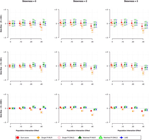
Figures 4 and 5 illustrate respectively for continuous and ordinal item score conditions, the mean bias in the estimate of the interaction between NA and SI for each of the 72 scenarios in our simulation study. Each figure shows nine plots, divided over three rows and three columns. The rows represent different sample sizes and the columns different amounts of skewness. Within each plot, the x-axis shows varying sizes of the true interaction between NA and SI. The y-axis shows the bias in the estimate of the standardized regression coefficients of the interaction between NA and SI. In each plot, the colors and shape of the data points correspond to different methods to model the interaction effect. Each dot corresponds to the bias in the parameter estimate averaged over 500 replications and the error bars represent the 95% confidence interval of the mean.

Figure 4. Comparison of four methods to estimate interaction effects between NA and SI on depression in scenarios with continuous items, varying over the true interaction size (x-axis), amount of skewness (columns) and sample size (rows). Each data point shows the mean bias (including 95% confidence interval) in the standardized regression coefficient of the estimated interaction effect.

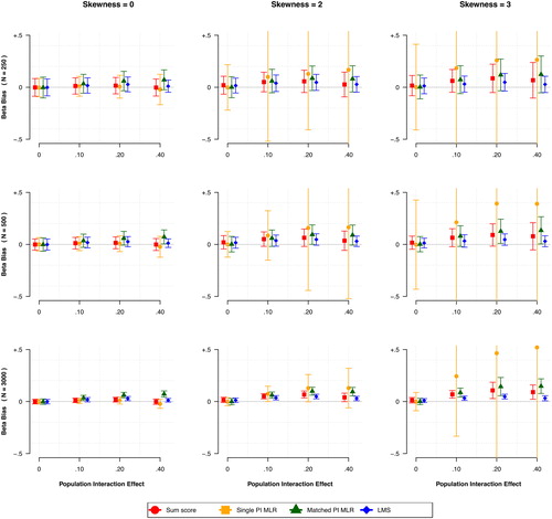
Figure 5. Comparison of four methods to estimate interaction effects between NA and SI on depression in scenarios with ordinal items, varying over the true interaction size (x-axis), amount of skewness (columns) and sample size (rows). Each data point shows the mean bias (including 95% confidence interval) in the standardized regression coefficient of the estimated interaction effect.

Continuous item scores

When comparing the four methods used on continuous item scores, Table 4 shows that the LMS MLR performed best across almost all conditions with respect to minimizing bias, followed by the Sum score approach, and Matched PI MLR. For all methods, the least-biased conditions were those with the largest sample size, a zero interaction effect, or no skewness. Overall, the bias tended to increase as the sample size decreased and as the skewness increased. Against our expectations, when skewness was present in the latent traits LMS performed best, while Single PI performed poorly.

Figure 4 illustrates that for all methods the average bias was mostly positive, implying that the interaction effect was overestimated in conditions with continuous item scores. For the LMS and Sum score methods, the size of the interaction did not have a large impact on the bias in the estimates. However, both PI methods overestimated the larger interaction effects, especially when skewness was present. Of all methods, LMS had the highest precision because it showed the least variability in the estimated interaction effects, as indicated by the narrowest confidence intervals in Figure 4. As expected, for all methods larger sample sizes reduced the variability in the estimated interaction effects across the 500 replications. An interesting finding is that higher skewness resulted in more variability in the estimated effects for all methods, but especially so for the Single PI MLR method.

Table 5 shows that the power to detect a significant interaction effect was above 0.80 for all methods in the continuous item score conditions, except for the Single PI MLR method. This method was especially underpowered as skewness increases, even at larger sample sizes, possibly because it resulted in widely varying estimates of the interaction effect, as indicated by the broad confidence intervals around the mean estimate of the interaction effect in conditions with skewness (Figure 4).

Table 5 further indicates for both the Single PI MLR and Matched PI MLR approaches were able to retain a false-positive rate of approximately 5% across all simulation conditions. Both the LMS and Sum score method also showed acceptable false-positive rates, but only when the latent traits were not skewed. As skewness increased, more false-positive findings emerged, and this effect was magnified with larger sample sizes.

Ordinal item scores

When comparing the six methods used on ordinal item scores, Table 4 shows that the LMS MLR performed best across almost all conditions with respect to minimizing bias, followed by the Sum score, Matched PI DWLS and Matched PI MLR approaches. For all methods, the least-biased conditions were those with the largest sample size and no skewness, and bias increased as the sample size decreased and as skewness increased. Both Single PI MLR and Single PI DWLS performed poorly with respect to the mean squared error, especially when skewness was present and as the true size of the interaction became larger. Contrary to our expectations, for skewed latent traits Matched PI MLR was slightly less biased than Matched PI DWLS. However, the Single PI DWLS did perform slightly better than Single PI MLR when skewness was present.

Figure 5 illustrates that for both Single PI methods the average bias was mostly negative, implying that these methods underestimated the interaction effect when item scores were ordinal. The average bias for the other methods depended on specific design factors. The bias of the LMS MLR and both Matched PI methods was largely similar, though without skewness LMS MLR was less biased than both Matched PI methods.

The width of the confidence intervals in Figure 5(A) indicates there were no large differences with respect to the precision of the six methods. Interestingly, the Single PI methods extremely variable estimates in skewed and continuous conditions did not apply to the ordinal conditions. As expected, for all methods larger sample sizes reduced the variability in the estimated interaction effects across the 500 replications. Higher skewness resulted in slightly more variability in the estimated effects for all methods.

Table 5 shows that for ordinal conditions, LMS outperformed the other methods with respect to maximizing the power to detect a significant interaction effect, followed closely by the Sum score method. As expected, for all methods the power increased with larger sample sizes and for N = 250 the Single PI MLR, Single PI DWLS and Matched PI MLR methods were underpowered to detect the smallest simulated effect. Increasing the sample size to N = 500 resulted in adequate power for all methods except the Single PI MLR method, still underpowered to detect the smallest effect.

With respect to minimizing the percentage of false-positive findings, Table 5 shows that the Single PI MLR method outperformed all other methods, but was closely followed by the Matched PI MLR method. These methods managed to keep the false-positive rate close to 5% in most conditions. Although they produced somewhat poorer false-positive rates when skewness and sample size were large, they still outperformed the other methods in those simulation conditions. While both the Single- and Matched PI DWLS methods never showed acceptable false-positive rates, the LMS and Sum score method only showed acceptable false-positive rates without skewness. Both the LMS and Sum score method showed an increase in false-positive rates as skewness increased, and this effect was most pronounced with larger sample sizes.

Discussion

In this study, we investigated the relation between Type D personality, depression, and anxiety using a latent prediction model. To our knowledge, the association between these constructs has not been analyzed previously with latent variable models that take into account the measurement error present in the scales that measure these constructs. These modeling approaches allowed us to prevent the kind of bias that is likely to occur when analyzing such data with regular regression analysis based on sum score variables (Busemeyer & Jones, 1983; Embretson, 1996; Kang & Waller, 2005; MacCallum, Zhang, Preacher, & Rucker, 2002).

In Study 1, we applied a latent prediction model to existing data of 3314 persons with Type 1 or 2 diabetes. Results according to six methods to model interaction effects suggested a small but significant effect of Type D personality (viz. an interaction of its subcomponents NA and SI) on depression and anxiety, implying that the association of negative affectivity with both depression and anxiety tends to get stronger as people show more social inhibition. These findings are consistent with earlier research that did not use latent variable modeling (Nefs et al., 2015). However, the inclusion of quadratic NA and SI effects to the models reduced the size of the interaction effect. Indeed, both Single PI methods produced smaller but still significant interaction effects, while for other methods the interaction effect either reduced to zero (Sum score; Matched PI MLR; Matched PI DWLS), or even changed in the opposite direction (LMS). Given these conflicting results, we conducted a Monte Carlo simulation study to investigate the bias and precision of each of the six methods used to model the interaction effect.

In our simulation study, we found that the six methods to model interaction effects differ in the accuracy and precision of the estimated interaction effects. In general, the LMS approach performed best with respect to minimizing bias in the estimated interaction effect. This conclusion applies both to continuous as well as ordinal item scores. Unexpectedly, when skewness was present in the latent traits LMS was the least-biased method, although it still overestimated the true value of the interaction on these occasions. This finding contrasts with earlier research showing the Matched PI approach to be less biased than LMS when skewness was present (Marsh et al., 2004; Kelava, Nagengast, & Brandt, 2014).

In general, the Single PI approach did not perform well in terms of minimizing bias. Especially when skewness was high and item scores were continuous this approach resulted in widely varying interaction effect estimates. This finding also applies to the Matched PI approach, yet to a much lesser extent. The worse performance of the Single PI method compared to the Matched PI method is not surprising, because the Single PI method has to rely on a single product indicator when estimating the interaction effect. In light of these findings, we strongly recommend against using the Single PI approach when modeling latent interaction effects.

With respect to maximizing the power to detect a nonzero interaction effect, LMS outperformed the other methods, both for continuous as well as for ordinal item scores. However, the Sum score approach and Matched PI approaches were also adequately powered in most simulated conditions. Regarding the percentage of false positives, the Single PI MLR and Matched PI MLR methods outperformed the other methods in most simulation conditions, keeping the false-positive rate around 5%. Both LMS and the sum score method were only able to control the false-positive rate without skewness in the latent traits. As the latent traits got more skewed, these methods produced more false positives. This is no surprise, given that these conditions fail to meet LMS’s assumption that the item scores of the exogenous latent variables show a multivariate normal distribution (Klein & Moosbrugger, 2000). These high power and the inflated false positive of the LMS approach are in line with findings from other simulation studies examining the LMS approach (Marsh et al., 2004; Kelava & Nagengast, 2012). Although the Single PI MLR and Matched PI MLR approach were able to better control the false-positive rate than LMS in simulation conditions with skewness, both PI approaches still performed worse than LMS in terms of bias and the power to detect a nonzero interaction effect.

Earlier research showed that for ordinal data, fitting a confirmatory factor model to the polychoric correlation matrix and estimating the parameters with (D)WLS estimation is fairly robust to moderate violations of the assumption that the underlying latent traits are normally distributed (Flora & Curran, 2004). Interestingly, our results indicated that for ordinal data, fitting the model to the polychoric correlation matrix (rather than the product moment correlation matrix) and using DWLS (rather than MLR estimation) was not beneficial with respect to minimizing the bias and false-positive conclusions, but did show slightly better power. Our results highlight that if one decides to use the Single- or Matched PI approaches, it is not necessary to use the categorical DWLS approach as the continuous MLR strategy performs at least as well, and is more parsimonious.

In terms of minimizing bias, the Sum score approach also performed reasonably well in general, being the second least-biased method, after LMS. Without skewness the Sum score approach even performed equally well as LMS, independent of whether the item scores were continuous or ordinal. We expected that the Sum score approach would show attenuated interaction effect estimates because this method does not take into account measurement error. However, the results of our simulation indicated that the Sum score approach overestimated the interaction effect. A possible explanation for this finding could be that ignoring measurement error can under some circumstances lead to overestimated associations, especially as models become more complex (Cole & Preacher, 2014). The Sum score approach resulted in spurious interactions only when skewness was high and/or sample size was large and this effect was more pronounced for ordinal than for continuous items. These results align with earlier research showing that the Sum score method can indeed lead to spurious interactions (Embretson, 1996; Schwabe & Van den Berg, 2014).

To the best of our knowledge, this is the first simulation study comparing the performance of the Sum score, LMS and PI approaches when modeling interactions between latent variables based on ordinal data. Based on our findings, we would advise researchers to use latent variable modeling when testing for interactions between variables that are measured with error. This echoes similar statements made over the years that highlight the importance of latent variable models in isolating a construct from its measurement error (Rasch, 1960; Birnbaum, 1968; Embretson, 1996; Kang & Waller, 2005; Schwabe & van den Berg, 2014). When comparing continuous with ordinal simulation conditions, LMS appears to perform slightly better when item scores are continuous, while the other methods perform better when item scores are ordinal. Nevertheless, if one aims to minimize bias in estimating the latent interaction effect, then we recommend to use the LMS approach, as this approach is the least biased across all simulation conditions, even when latent traits are skewed and item scores are ordinal. If one aims at maximizing the power to detect a nonzero interaction effect, then LMS is also the method of choice. However, LMS did show increased false-positive rates as the skewness of the latent traits increased. Both PI MLR approaches adequately kept the false-positive rate close to 5%. Of those two, the Matched PI MLR approach appears much less biased than the Single PI MLR approach. Therefore, if one aims at minimizing the chance on false-positive findings, one could consider using the Matched PI MLR approach. This conclusion resonates with earlier research showing the benefits of this particular method relative to other methods to construct latent interactions (Marsh, Wen, & Hau, 2004; Cham, West, Ma, & Aiken, 2012).

Although our simulation showed LMS to be the least-biased method, it still overestimated the interaction effect and has an inflated false-positive rate when the latent traits were skewed, especially when item scores were ordinal. This aligns with earlier research indicating that LMS shows biased parameter estimates when skewness is introduced (Kelava & Nagengast, 2012; Kelava, Nagengast, & Brandt, 2014; Cham, West, Ma, & Aiken, 2012). Other promising methods that fell beyond the scope of the present study use mixture modeling to model skewed exogenous latent variables (Dolan & Van der Maas, 1998). For instance, the recently developed Nonlinear Structural Equation Mixture Modeling (Kelava, Nagengast, & Brandt, 2014) and the Bayesian finite mixture model (Kelava & Nagengast, 2012) both show promise in modeling latent interaction and quadratic effects when the latent exogenous variables are not normally distributed. However, it is unclear how these methods perform when item scores are ordinal rather than continuous. This would be an interesting avenue for future research.

The primary motivation for our simulation study was to place the results of our empirical study in context, assessing the bias and precision of the six methods used to model interaction effects. Of all simulation conditions, the one with a sample size of 3000, ordinal item scores, skewed latent traits, and an interaction effect of .207 most resembles the circumstances of our empirical study. Interestingly, our simulation study indicated that the Sum score approach is least biased in that specific scenario. This method showed that the interaction between NA and SI is no longer statistically significant after adding the quadratic NA and SI effects to the model. However, in the simulations, the Sum score approach exhibited many false positives when latent traits were skewed and item scores were ordinal. To lower the possibility that the significant quadratic NA and SI effects reflect false-positive findings, we can inspect the results of the Matched PI MLR approach, which showed nominal false-positive rates close to 5%. The empirical results of the Matched PI MLR approach are also similar to those of the Sum score method: adding the significant quadratic NA and SI effects to the model rendered the interaction between NA and SI statistically insignificant.

Combined, our findings fail to support our main hypothesis that the association between negative affectivity and both depression and anxiety gets stronger at higher levels of social inhibition. Rather, our results suggest that the effect of NA on both depression and anxiety might get stronger at higher levels of NA, and that there exist a similar but smaller quadratic effect for SI on both depression and anxiety. Effects similar to these have been reported in earlier research, where the personality traits neuroticism (correlation with NA: r = 0.68; de Fruyt & Denollet, 2002) and introversion (correlation with SI: r = 0.52; de Fruyt & Denollet, 2002) did not show a significant interaction on depression and anxiety, yet both did show significant quadratic effects (Jorm et al., 2000). Quadratic effects are known to be well-approximated by interaction effects, especially as the constructs involved in the interaction correlate highly (Kang & Waller, 2005). Therefore, in line with other researchers, we stress the importance of always first adding the quadratic effects to models that test for the presence of interaction effects (Lubinski & Humphreys, 1990).

Our study investigated the association between Type D personality and anxiety and depression. Apart from these clinical psychological constructs, there exists a large body of research investigating whether Type D personality is related to worse health-related outcomes in the general population (Mols & Denollet, 2010) or in people with cardiovascular disease (Denollet et al., 2010, 2018). Because most of these studies did not apply latent variable modeling and did not test for quadratic NA and SI effects, an interesting avenue for future research would be to do so in preregistered, highly powered direct replication projects. Such studies will not only highlight the importance of latent variable modeling, but also answer recent critiques (e.g., Smith, 2011; Grande, Romppel, & Barth, 2012) questioning the replicability of research on Type D personality (for a more detailed discussion of this issue, see Denollet et al., 2013).

Finally, we would like to note that the methods used in this study are not limited to research on Type D personality. The investigated approaches to model latent interactions can be readily applied to future studies aimed at accounting for measurement error while analyzing interactions between psychological constructs.

Article Information

Conflict of interest disclosures: Each author signed a form for disclosure of potential conflicts of interest. No authors reported any financial or other conflicts of interest in relation to the work described.

Ethical principles: The authors affirm having followed professional ethical guidelines in preparing this work. These guidelines include obtaining informed consent from human participants, maintaining ethical treatment and respect for the rights of human or animal participants, and ensuring the privacy of participants and their data, such as ensuring that individual participants cannot be identified in reported results or from publicly available original or archival data.

Funding: The research of JMW is supported by a Consolidator Grant (IMPROVE) from the European Research Council (ERC; grant no. 726361).

Role of the funders/sponsors: None of the funders or sponsors of this research had any role in the design and conduct of the study; collection, management, analysis, and interpretation of data; preparation, review, or approval of the manuscript; or decision to submit the manuscript for publication.

Acknowledgments: The authors would like to thank Marjan Bakker, Angelique Cramer, Elise Crompvoets, Inga Schwabe, Jesper Tijmstra and Eva Zijlmans for their comments on prior versions of this article. The ideas and opinions expressed herein are those of the authors alone, and endorsement by the authors’ institutions or the funding agency is not intended and should not be inferred.

Notes

1 For instance, because the BIC is based on the log likelihood, Mplus only reports this fit index for models involving maximum likelihood estimation. Consequently, this fit index is not reported for our models involving weighted least squares estimation. Furthermore, when numerical integration is required (e.g., with the LMS method), means, variances, and covariances are not sufficient statistics for model estimation and chi-square and related fit statistics are not available. As a result, Mplus does for the LMS method not report the chi-square statistics and related indices (RMSEA, CFI, and TLI).

2 Originally, we compared these two models with a log-likelihood difference test. However, the resulting chi-square difference value was negative, and thus the test is invalid as these tests should result in a positive chi-square difference. We may add that such negative chi-square values can arise when using MLR estimation. As an alternative, we used the Wald test, which is available in MPLUS, to test the constraint that both interaction effects are equal to zero.

3 We used the parameter estimates resulting from the LMS method, because this is the default method in Mplus to model interaction effects.

Appendix A. DS14 scale information for study 1.

Table

DS14	Negative affectivity							Social inhibition
	DS2	DS4	DS5	DS7	DS9	DS12	DS13	DS1	DS3	DS6	DS8	DS10	DS11	DS14
DS2	1
DS4	0.35	1
DS5	0.43	0.52	1
DS7	0.45	0.64	0.54	1
DS9	0.36	0.51	0.6	0.57	1
DS12	0.52	0.6	0.54	0.68	0.51	1
DS13	0.4	0.71	0.51	0.73	0.58	0.72	1
DS1	0.09	0.23	0.16	0.27	0.24	0.21	0.24	1
DS3	0.05	0.15	0.1	0.18	0.18	0.15	0.14	0.63	1
DS6	0.32	0.46	0.39	0.5	0.42	0.44	0.46	0.54	0.4	1
DS8	0.22	0.31	0.27	0.39	0.36	0.32	0.33	0.64	0.51	0.64	1
DS10	0.12	0.3	0.26	0.33	0.35	0.3	0.31	0.57	0.45	0.52	0.55	1
DS11	0.19	0.34	0.33	0.4	0.4	0.38	0.38	0.51	0.42	0.53	0.53	0.66	1
DS14	0.2	0.37	0.29	0.4	0.39	0.36	0.4	0.59	0.47	0.63	0.7	0.56	0.56	1
Skewness	0.11	0.79	0.18	0.63	0.86	0.25	0.93	0.67	0.22	0.48	0.62	0.45	0.37	0.72
Kurtosis	−0.97	−0.37	−0.92	−0.67	−0.08	−1.07	−0.1	−0.32	−0.76	−0.83	−0.69	−1.02	−0.92	−0.47

Appendix B. PHQ-9 & GAD-7 scale information for study 1.

Table

	PHQ9_1	PHQ9_2	PHQ9_3	PHQ9_4	PHQ9_5	PHQ9_6	PHQ9_7	PHQ9_8	PHQ9_9
PHQ9_1	1
PHQ9_2	0.72	1
PHQ9_3	0.42	0.44	1
PHQ9_4	0.54	0.52	0.55	1
PHQ9_5	0.44	0.45	0.4	0.48	1
PHQ9_6	0.53	0.64	0.36	0.43	0.45	1
PHQ9_7	0.49	0.51	0.38	0.49	0.39	0.46	1
PHQ9_8	0.39	0.43	0.33	0.37	0.34	0.4	0.48	1
PHQ9_9	0.38	0.48	0.22	0.27	0.29	0.43	0.3	0.26	1
Skewness	1.66	2.06	0.93	0.73	1.94	2.19	1.77	3.1	4.99
Kurtosis	2.63	4.28	–0.22	–0.5	3.2	4.4	2.66	10.19	29.49

Appendix C. Mean standardized regression coefficient (including 95% confidence interval) of the interaction effect between NA and SI on depression for all continuous simulation scenarios.

Table

				Latent variable models
N	Skewness	Size interaction	Sum score regression	LMS MLR	Single PI MLR	Matched PI MLR
250	0	0	0 [−.08/.08]	0 [−.08/.08]	0 [−.1/.1]	0 [−.1/.1]
		.1035	.12 [.04/.2]	.12 [.04/.2]	.11 [.01/.21]	.14 [.04/.24]
		.207	.22 [.14/.3]	.23 [.15/.31]	.21 [.09/.33]	.27 [.17/.37]
		.414	.41 [.33/.49]	.42 [.36/.48]	.39 [.25/.53]	.49 [.39/.59]
	2	0	.02 [−.06/.1]	.02 [−.06/.1]	0 [−.22/.22]	0 [−.1/.1]
		.1035	.15 [.05/.25]	.14 [.06/.22]	.2 [−.43/.83]	.16 [.04/.28]
		.207	.26 [.16/.36]	.25 [.17/.33]	.34 [−.19/.87]	.29 [.17/.41]
		.414	.44 [.32/.56]	.44 [.36/.52]	.58 [−.48/1.64]	.49 [.37/.61]
	3	0	.02 [−.08/.12]	.01 [−.07/.09]	0 [−.41/.41]	0 [−.12/.12]
		.1035	.16 [.04/.28]	.13 [.05/.21]	.29 [−.81/1.39]	.18 [.04/.32]
		.207	.29 [.15/.43]	.26 [.18/.34]	.47 [−.71/1.65]	.33 [.17/.49]
		.414	.48 [.3/.66]	.44 [.36/.52]	.68 [−.81/2.17]	.54 [.36/.72]
500	0	0	0 [−.06/.06]	0 [−.06/.06]	0 [−.06/.06]	0 [−.06/.06]
		.1035	.12 [.06/.18]	.12 [.06/.18]	.11 [.05/.17]	.14 [.08/.2]
		.207	.22 [.16/.28]	.23 [.19/.27]	.21 [.13/.29]	.27 [.21/.33]
		.414	.41 [.35/.47]	.43 [.39/.47]	.39 [.29/.49]	.49 [.43/.55]
	2	0	.02 [−.04/.08]	.02 [−.04/.08]	0 [−.12/.12]	0 [−.08/.08]
		.1035	.15 [.07/.23]	.14 [.08/.2]	.19 [−.05/.43]	.16 [.08/.24]
		.207	.27 [.19/.35]	.25 [.19/.31]	.37 [−.24/.98]	.3 [.2/.4]
		.414	.45 [.35/.55]	.44 [.38/.5]	.58 [−.11/1.27]	.5 [.4/.6]
	3	0	.02 [−.04/.08]	.01 [−.03/.05]	0 [−.43/.43]	0 [−.08/.08]
		.1035	.17 [.09/.25]	.14 [.08/.2]	.32 [−.74/1.38]	.18 [.08/.28]
		.207	.3 [.2/.4]	.25 [.19/.31]	.6 [−.97/2.17]	.33 [.21/.45]
		.414	.49 [.35/.63]	.44 [.38/.5]	.8 [−.75/2.35]	.55 [.41/.69]
3000	0	0	0 [−.02/.02]	0 [−.02/.02]	0 [−.02/.02]	0 [−.02/.02]
		.1035	.11 [.09/.13]	.12 [.1/.14]	.11 [.09/.13]	.14 [.12/.16]
		.207	.22 [.2/.24]	.24 [.22/.26]	.22 [.18/.26]	.27 [.25/.29]
		.414	.41 [.39/.43]	.43 [.41/.45]	.39 [.35/.43]	.49 [.45/.53]
	2	0	.02 [0/.04]	.01 [−.01/.03]	0 [−.04/.04]	0 [−.04/.04]
		.1035	.15 [.13/.17]	.14 [.12/.16]	.18 [.1/.26]	.17 [.13/.21]
		.207	.27 [.23/.31]	.26 [.24/.28]	.34 [.2/.48]	.31 [.27/.35]
		.414	.45 [.41/.49]	.44 [.42/.46]	.54 [.34/.74]	.51 [.47/.55]
	3	0	.01 [−.01/.03]	.01 [−.01/.03]	0 [−.08/.08]	0 [−.04/.04]
		.1035	.17 [.13/.21]	.14 [.12/.16]	.35 [−.22/.92]	.19 [.15/.23]
		.207	.31 [.23/.39]	.25 [.23/.27]	.67 [−.6/1.94]	.35 [.27/.43]
		.414	.5 [.42/.58]	.45 [.43/.47]	.93 [−.21/2.07]	.56 [.48/.64]

Appendix D. Mean standardized regression coefficient (including 95% confidence interval) of the interaction effect between NA and SI on depression for all ordinal simulation scenarios.

Table

N	Skewness	Size interaction		Latent variable models
			Sum score regression	LMS MLR	Single PI MLR	Single PI DWLS	Matched PI MLR	Matched PI DWLS
250	0	0	0 [−.08/.08]	0 [−.08/.08]	0 [−.08/.08]	0 [−.08/.08]	0 [−.1/.1]	0 [−.1/.1]
		.1035	.11 [.03/.19]	.12 [.04/.2]	.08 [0/.16]	.08 [0/.16]	.14 [.04/.24]	.13 [.03/.23]
		.207	.21 [.13/.29]	.23 [.15/.31]	.15 [.07/.23]	.15 [.07/.23]	.26 [.16/.36]	.25 [.15/.35]
		.414	.38 [.3/.46]	.41 [.33/.49]	.27 [.17/.37]	.27 [.17/.37]	.47 [.37/.57]	.46 [.36/.56]
	2	0	.03 [−.07/.13]	.04 [−.06/.14]	.01 [−.07/.09]	.01 [−.07/.09]	.01 [−.11/.13]	.03 [−.09/.15]
		.1035	.14 [.04/.24]	.15 [.07/.23]	.07 [−.01/.15]	.08 [0/.16]	.15 [.03/.27]	.16 [.04/.28]
		.207	.22 [.14/.3]	.24 [.14/.34]	.12 [.04/.2]	.12 [.04/.2]	.24 [.14/.34]	.25 [.13/.37]
		.414	.33 [.25/.41]	.37 [.27/.47]	.18 [.1/.26]	.19 [.09/.29]	.37 [.27/.47]	.38 [.26/.5]
	3	0	.03 [−.07/.13]	.04 [−.06/.14]	0 [−.08/.08]	.01 [−.07/.09]	.01 [−.13/.15]	.03 [−.09/.15]
		.1035	.14 [.04/.24]	.15 [.07/.23]	.06 [−.02/.14]	.07 [−.01/.15]	.15 [.03/.27]	.16 [.04/.28]
		.207	.22 [.14/.3]	.23 [.13/.33]	.11 [.03/.19]	.11 [.03/.19]	.24 [.12/.36]	.25 [.13/.37]
		.414	.32 [.22/.42]	.36 [.24/.48]	.16 [.08/.24]	.17 [.07/.27]	.36 [.24/.48]	.37 [.25/.49]
500	0	0	0 [−.06/.06]	0 [−.06/.06]	0 [−.06/.06]	0 [−.06/.06]	0 [−.08/.08]	0 [−.08/.08]
		.1035	.11 [.05/.17]	.12 [.06/.18]	.08 [.02/.14]	.07 [.01/.13]	.14 [.06/.22]	.13 [.07/.19]
		.207	.21 [.15/.27]	.23 [.17/.29]	.15 [.09/.21]	.15 [.09/.21]	.26 [.18/.34]	.25 [.17/.33]
		.414	.38 [.32/.44]	.41 [.35/.47]	.27 [.19/.35]	.26 [.18/.34]	.47 [.39/.55]	.46 [.38/.54]
	2	0	.03 [−.03/.09]	.04 [−.02/.1]	.01 [−.05/.07]	.01 [−.05/.07]	.01 [−.09/.11]	.03 [−.05/.11]
		.1035	.14 [.08/.2]	.15 [.09/.21]	.07 [.01/.13]	.08 [.02/.14]	.15 [.07/.23]	.16 [.08/.24]
		.207	.22 [.16/.28]	.24 [.18/.3]	.12 [.06/.18]	.12 [.06/.18]	.24 [.16/.32]	.25 [.17/.33]
		.414	.33 [.27/.39]	.37 [.31/.43]	.18 [.12/.24]	.19 [.13/.25]	.37 [.29/.45]	.38 [.3/.46]
	3	0	.04 [−.04/.12]	.04 [−.02/.1]	.01 [−.05/.07]	.01 [−.05/.07]	.02 [−.08/.12]	.03 [−.07/.13]
		.1035	.14 [.08/.2]	.15 [.09/.21]	.07 [.01/.13]	.07 [.01/.13]	.15 [.07/.23]	.16 [.08/.24]
		.207	.22 [.16/.28]	.23 [.17/.29]	.1 [.04/.16]	.11 [.05/.17]	.24 [.16/.32]	.24 [.16/.32]
		.414	.31 [.25/.37]	.35 [.27/.43]	.16 [.1/.22]	.17 [.11/.23]	.35 [.27/.43]	.37 [.29/.45]
3000	0	0	0 [−.02/.02]	0 [−.02/.02]	0 [−.02/.02]	0 [−.02/.02]	0 [−.02/.02]	0 [−.02/.02]
		.1035	.11 [.09/.13]	.12 [.1/.14]	.08 [.06/.1]	.08 [.06/.1]	.14 [.1/.18]	.13 [.09/.17]
		.207	.21 [.19/.23]	.23 [.21/.25]	.15 [.13/.17]	.15 [.13/.17]	.26 [.24/.28]	.25 [.21/.29]
		.414	.38 [.36/.4]	.41 [.39/.43]	.27 [.23/.31]	.27 [.23/.31]	.46 [.42/.5]	.46 [.44/.48]
	2	0	.03 [.01/.05]	.04 [.02/.06]	.01 [−.01/.03]	.01 [−.01/.03]	.01 [−.03/.05]	.03 [−.01/.07]
		.1035	.14 [.12/.16]	.15 [.13/.17]	.07 [.05/.09]	.08 [.06/.1]	.14 [.1/.18]	.16 [.12/.2]
		.207	.22 [.2/.24]	.24 [.22/.26]	.12 [.1/.14]	.12 [.1/.14]	.24 [.22/.26]	.25 [.23/.27]
		.414	.33 [.31/.35]	.37 [.35/.39]	.18 [.16/.2]	.19 [.17/.21]	.37 [.35/.39]	.38 [.36/.4]
	3	0	.04 [.02/.06]	.04 [.02/.06]	.01 [−.01/.03]	.01 [−.01/.03]	.01 [−.03/.05]	.03 [−.01/.07]
		.1035	.14 [.12/.16]	.15 [.13/.17]	.06 [.04/.08]	.07 [.05/.09]	.15 [.11/.19]	.15 [.11/.19]
		.207	.22 [.2/.24]	.23 [.21/.25]	.1 [.08/.12]	.11 [.09/.13]	.23 [.19/.27]	.24 [.2/.28]
		.414	.31 [.29/.33]	.35 [.31/.39]	.16 [.12/.2]	.17 [.15/.19]	.35 [.31/.39]	.37 [.33/.41]

Appendix E. For each simulation condition, the squared distance between the estimated value of the interaction effect and the true value of the interaction, averaged across 500 replications (mean squared error).

Table

N	Skewness	True size interaction	Continuous item scores				Ordinal item scores
			Sum score	LMS	Single	Matched	Sum score	LMS	Single PI		Matched PI
			regression	MLR	PI MLR	PI MLR	regression	MLR	MLR	WLS	MLR	WLS
250	0	0	0.002	0.002	0.002	0.003	0.002	0.002	0.002	0.001	0.003	0.003
		.1035	0.002	0.002	0.002	0.003	0.002	0.002	0.002	0.002	0.004	0.004
		.207	0.002	0.002	0.003	0.006	0.002	0.002	0.005	0.005	0.006	0.004
		.414	0.002	0.001	0.006	0.007	0.003	0.001	0.022	0.024	0.006	0.005
	1	0	0.002	0.002	0.012	0.003	0.003	0.004	0.001	0.002	0.004	0.005
		.1035	0.005	0.003	0.11	0.007	0.004	0.004	0.003	0.002	0.005	0.006
		.207	0.006	0.004	0.092	0.011	0.002	0.003	0.01	0.009	0.004	0.005
		.414	0.004	0.002	0.319	0.011	0.01	0.004	0.058	0.053	0.005	0.004
	2	0	0.003	0.002	0.044	0.003	0.004	0.004	0.001	0.002	0.004	0.005
		.1035	0.007	0.002	0.348	0.01	0.004	0.004	0.003	0.002	0.005	0.006
		.207	0.012	0.004	0.428	0.02	0.002	0.003	0.012	0.011	0.005	0.005
		.414	0.012	0.002	0.652	0.023	0.011	0.006	0.066	0.061	0.007	0.006
500	0	0	0.001	0.001	0.001	0.001	0.001	0.001	0.001	0.001	0.001	0.001
		.1035	0.001	0.001	0.001	0.002	0.001	0.001	0.001	0.002	0.002	0.002
		.207	0.001	0.001	0.002	0.005	0.001	0.001	0.004	0.004	0.004	0.003
		.414	0.001	0.001	0.003	0.006	0.002	0.001	0.022	0.024	0.004	0.003
	1	0	0.001	0.001	0.004	0.001	0.002	0.003	0.001	0.001	0.002	0.003
		.1035	0.004	0.002	0.022	0.005	0.003	0.003	0.002	0.002	0.003	0.004
		.207	0.006	0.003	0.119	0.011	0.001	0.002	0.009	0.008	0.003	0.003
		.414	0.004	0.002	0.149	0.01	0.008	0.003	0.056	0.051	0.003	0.002
	2	0	0.001	0.001	0.048	0.001	0.003	0.003	0.001	0.001	0.002	0.003
		.1035	0.006	0.002	0.336	0.009	0.003	0.003	0.002	0.002	0.003	0.004
		.207	0.011	0.003	0.799	0.019	0.001	0.001	0.011	0.01	0.003	0.003
		.414	0.011	0.002	0.777	0.023	0.011	0.005	0.066	0.06	0.005	0.004
3000	0	0	0	0	0	0	0	0	0	0	0	0
		.1035	0	0	0	0.001	0	0	0.001	0.001	0.001	0.001
		.207	0	0.001	0	0.004	0	0.001	0.003	0.003	0.003	0.003
		.414	0	0	0.001	0.005	0.001	0	0.02	0.022	0.003	0.002
	1	0	0	0	0	0	0.001	0.002	0	0	0	0.001
		.1035	0.003	0.001	0.007	0.004	0.002	0.002	0.001	0.001	0.002	0.003
		.207	0.005	0.002	0.021	0.01	0	0.001	0.009	0.007	0.001	0.002
		.414	0.002	0.001	0.026	0.009	0.008	0.002	0.056	0.051	0.002	0.001
	2	0	0	0	0.002	0	0.001	0.002	0	0	0.001	0.001
		.1035	0.005	0.001	0.146	0.008	0.002	0.002	0.002	0.001	0.002	0.003
		.207	0.013	0.002	0.632	0.023	0	0.001	0.011	0.009	0.001	0.002
		.414	0.009	0.001	0.609	0.023	0.01	0.004	0.066	0.06	0.004	0.002

Table

	GAD7_1	GAD7_2	GAD7_3	GAD7_4	GAD7_5	GAD7_6	GAD7_7
GAD7_1	1
GAD7_2	0.71	1
GAD7_3	0.68	0.77	1
GAD7_4	0.67	0.66	0.67	1
GAD7_5	0.49	0.48	0.47	0.58	1
GAD7_6	0.51	0.5	0.52	0.57	0.48	1
GAD7_7	0.52	0.54	0.53	0.46	0.37	0.42	1
Skewness	1.76	2.06	1.44	1.5	2.26	1.36	2.62
Kurtosis	3.27	4.34	2.02	1.99	5.41	1.81	7.42

References

- Asparouhov, T., & Muthén, B. (2010). Simple second order chi-square correction. Mplus Technical Appendix.
- Babakus, E., Ferguson, C. E., Jr., & Jöreskog, K. G. (1987). The sensitivity of confirmatory maximum likelihood factor analysis to violations of measurement scale and distributional assumptions. Journal of Marketing Research, 37, 222–228. doi:10.2307/3151512
- Birnbaum, A. (1968). Some latent trait models and their use in inferring an examinee’s ability. In F. M. Lord & M. R. Novick (Eds.), Statistical theories of mental test scores (pp. 397–479). Reading, MA: Addison-Wesley.
- Bollen, K. A. (1989). Structural equations with latent variables. New York: John Wiley & Sons.
- Bollen, K. A., & Stine, R. A. (1993). Bootstrapping goodness-of-fit measures in structural equation models. Sociological Methods & Research, 21(2), 205–229. doi:10.1177/0049124192021002004
- Borsboom, D., Mellenbergh, G. J., & Van Heerden, J. (2003). The theoretical status of latent variables. Psychological Review, 110(2), 203. doi:10.1037/0033-295X.110.2.203
- Browne, M. W. (1984). Asymptotically distribution‐free methods for the analysis of covariance structures. British Journal of Mathematical and Statistical Psychology, 37(1), 62–83. doi:10.1111/j.2044-8317.1984.tb00789.x
- Busemeyer, J. R., & Jones, L. E. (1983). Analysis of multiplicative combination rules when the causal variables are measured with error. Psychological Bulletin, 93(3), 549. doi:10.1037/0033-2909.93.3.549
- Cham, H., West, S. G., Ma, Y., & Aiken, L. S. (2012). Estimating latent variable interactions with nonnormal observed data: A comparison of four approaches. Multivariate Behavioral Research, 47(6), 840–876. doi:10.1080/00273171.2012.732901
- Chen, F., Curran, P. J., Bollen, K. A., Kirby, J., & Paxton, P. (2008). An empirical evaluation of the use of fixed cutoff points in RMSEA test statistic in structural equation models. Sociological methods & research, 36(4), 462–494.
- Cole, D. A., & Preacher, K. J. (2014). Manifest variable path analysis: Potentially serious and misleading consequences due to uncorrected measurement error. Psychological Methods, 19(2), 300. doi:10.1037/a0033805
- Coyne, J. C., Jaarsma, T., Luttik, M. L., van Sonderen, E., van Veldhuisen, D. J., & Sanderman, R. (2011). Lack of prognostic value of Type D personality for mortality in a large sample of heart failure patients. Psychosomatic Medicine, 73(7), 557–562. doi:10.1097/PSY.0b013e318227ac75
- De Fruyt, F., & Denollet, J. (2002). Type D personality: A five-factor model perspective. Psychology and Health, 17(5), 671–683. doi:10.1080/08870440290025858
- Denollet, J. (2005). DS14: standard assessment of negative affectivity, social inhibition, and Type D personality. Psychosomatic Medicine, 67(1), 89–97. doi:10.1097/01.psy.0000149256.81953.49
- Denollet, J., Pedersen, S. S., Vrints, C. J., & Conraads, V. M. (2013). Predictive value of social inhibition and negative affectivity for cardiovascular events and mortality in patients with coronary artery disease: The Type D personality construct. Psychosomatic Medicine, 75(9), 873–881. http://dx.doi.org/10.1016/S0140-6736(96)90007-0 doi:10.1097/PSY.0000000000000001
- Denollet, J., Schiffer, A. A., & Spek, V. (2010). A general propensity to psychological distress affects cardiovascular outcomes evidence from research on the Type D (distressed) personality profile. Circulation: cardiovascular Quality and Outcomes, 3(5), 546–557. doi:10.1161/CIRCOUTCOMES.109.934406
- Denollet, J., van Felius, R. A., Lodder, P., Mommersteeg, P. M., Goovaerts, I., Possemiers, N., … Van Craenenbroeck, E. M. (2018). Predictive value of Type D personality for impaired endothelial function in patients with coronary artery disease. International Journal of Cardiology, 259, 205–210. doi:10.1016/j.ijcard.2018.02.064
- Dolan, C. V. (1994). Factor analysis of variables with 2, 3, 5 and 7 response categories: A comparison of categorical variable estimators using simulated data. British Journal of Mathematical and Statistical Psychology, 47(2), 309–326. doi:10.1111/j.2044-8317.1994.tb01039.x
- Dolan, C. V., & van der Maas, H. L. (1998). Fitting multivariage normal finite mixtures subject to structural equation modeling. Psychometrika, 63(3), 227–253. doi:10.1007/BF02294853
- Embretson, S. E. (1996). Item response theory models and spurious interaction effects in factorial ANOVA designs. Applied Psychological Measurement, 20(3), 201–212. doi:10.1177/014662169602000302
- Flora, D. B., & Curran, P. J. (2004). An empirical evaluation of alternative methods of estimation for confirmatory factor analysis with ordinal data. Psychological Methods, 9(4), 466. doi:10.1037/1082-989X.9.4.466
- Flora, D. B., LaBrish, C., & Chalmers, R. P. (2012). Old and new ideas for data screening and assumption testing for exploratory and confirmatory factor analysis. Frontiers in Psychology, 3, 55. http://dx.doi.org/10.3389/fpsyg.2012.00055
- Forero, C. G., & Maydeu-Olivares, A. (2009). Estimation of IRT graded response models: Limited versus full information methods. Psychological Methods, 14(3), 275. doi:10.1037/a0015825
- Frasure-Smith, N., & Lespérance, F. (2008). Depression and anxiety as predictors of 2-year cardiac events in patients with stable coronary artery disease. Archives of General Psychiatry, 65(1), 62–71. doi:10.1001/archgenpsychiatry.2007.4
- Grande, G., Romppel, M., & Barth, J. (2012). Association between Type D personality and prognosis in patients with cardiovascular diseases: A systematic review and meta-analysis. Annals of Behavioral Medicine, 43(3), 299–310. doi:10.1007/s12160-011-9339-0
- Grande, G., Romppel, M., Vesper, J. M., Schubmann, R., Glaesmer, H., & Herrmann-Lingen, C. (2011). Type D personality and all-cause mortality in cardiac patients-data from a German cohort study. Psychosomatic Medicine, 73(7), 548–556. doi:10.1097/PSY.0b013e318227a9bc
- Hallquist, M., & Wiley, J. (2011). MplusAutomation: Automating Mplus model estimation and interpretation. R package version 0.6. Retrieved from http://cran.r-project.org/web/packages/MplusAutomation/index.html
- Hambleton, R. K., Swaminathan, H., & Rogers, H. J. (1991). Fundamentals of item response theory (Vol. 2). Thousand Oaks, CA: Sage.
- ten Holt, J. C. T., van Duijn, M. A., & Boomsma, A. (2010). Scale construction and evaluation in practice: A review of factor analysis versus item response theory applications. Psychological Test and Assessment Modeling, 52(3), 272–297.
- Hu, L. T., & Bentler, P. M. (1999). Cutoff criteria for fit indexes in covariance structure analysis: Conventional criteria versus new alternatives. Structural Equation Modeling: A Multidisciplinary Journal, 6(1), 1–55. doi:10.1080/10705519909540118
- Jorm, A. F., Christensen, H., Henderson, A. S., Jacomb, P. A., Korten, A. E., & Rodgers, B. (2000). Predicting anxiety and depression from personality: Is there a synergistic effect of neuroticism and extraversion? Journal of Abnormal Psychology, 109(1), 145. doi:10.1037/0021-843X.109.1.145
- Kang, S. M., & Waller, N. G. (2005). Moderated multiple regression, spurious interaction effects, and IRT. Applied Psychological Measurement, 29(2), 87–105. doi:10.1177/0146621604272737
- Kelava, A., & Nagengast, B. (2012). A Bayesian model for the estimation of latent interaction and quadratic effects when latent variables are non-normally distributed. Multivariate Behavioral Research, 47(5), 717–742. doi:10.1080/00273171.2012.715560
- Kelava, A., Nagengast, B., & Brandt, H. (2014). A nonlinear structural equation mixture modeling approach for nonnormally distributed latent predictor variables. Structural Equation Modeling, 21(3), 468–481. doi:10.1080/10705511.2014.915379
- Kenny, D. A., & Judd, C. M. (1984). Estimating the nonlinear and interactive effects of latent variables. Psychological Bulletin, 96(1), 201. doi:10.1037/0033-2909.96.1.201
- Kline, R. B. (2011). Principles and practice of structural equation modeling. New York: Guilford Press.
- Klein, A., & Moosbrugger, H. (2000). Maximum likelihood estimation of latent interaction effects with the LMS method. Psychometrics, 65(4), 457–474. doi:10.1007/BF02296338
- Kroenke, K., Spitzer, R. L., & Williams, J. B. (2001). The PHQ-9: validity of a brief depression severity measure. Journal of General Internal Medicine, 16(9), 606–613. doi:10.1046/j.1525-1497.2001.016009606.x
- Kubzansky, L. D., Cole, S. R., Kawachi, I., Vokonas, P., & Sparrow, D. (2006). Shared and unique contributions of anger, anxiety, and depression to coronary heart disease: a prospective study in the normative aging study. Annals of Behavioral Medicine, 31(1), 21–29. doi:10.1207/s15324796abm3101_5
- Kupper, N., & Denollet, J. (2007). Type D personality as a prognostic factor in heart disease: Assessment and mediating mechanisms. Journal of Personality Assessment, 89(3), 265–276. doi:10.1080/00223890701629797
- Kupper, N., & Denollet, J. (2016). Explaining heterogeneity in the predictive value of Type D personality for cardiac events and mortality. International Journal of Cardiology, 224, 119–124. http://dx.doi.org/10.1016/j.ijcard.2016.09.006
- Kupper, N., Denollet, J., Widdershoven, J., & Kop, W. J. (2013). Type D personality is associated with low cardiovascular reactivity to acute mental stress in heart failure patients. International Journal of Psychophysiology, 90(1), 44–49. doi:10.1016/j.ijpsycho.2013.01.011
- Löwe, B., Decker, O., Müller, S., Brähler, E., Schellberg, D., Herzog, W., & Herzberg, P. Y. (2008). Validation and standardization of the Generalized Anxiety Disorder Screener (GAD-7) in the general population. Medical Care, 46(3), 266–274. doi:10.1097/MLR.0b013e318160d093
- Lubinski, D., & Humphreys, L. G. (1990). Assessing spurious “moderator effects”: Illustrated substantively with the hypothesized (“synergistic”) relation between spatial and mathematical ability. Psychological Bulletin, 107(3), 385. doi:10.1037/0033-2909.107.3.385
- MacCallum, R. C., & Mar, C. M. (1995). Distinguishing between moderator and quadratic effects in multiple regression. Psychological Bulletin, 118(3), 405. doi:10.1037/0033-2909.118.3.405
- MacCallum, R. C., Zhang, S., Preacher, K. J., & Rucker, D. D. (2002). On the practice of dichotomization of quantitative variables. Psychological Methods, 7(1), 19. doi:10.1037/1082-989X.7.1.19
- Marsh, H. W., Wen, Z., & Hau, K. T. (2004). Structural equation models of latent interactions: Evaluation of alternative estimation strategies and indicator construction. Psychological Methods, 9(3), 275. doi:10.1037/1082-989X.9.3.275
- Martin, A., Rief, W., Klaiberg, A., & Braehler, E. (2006). Validity of the brief patient health questionnaire mood scale (PHQ-9) in the general population. General Hospital Psychiatry, 28(1), 71–77. doi:10.1016/j.genhosppsych.2005.07.003
- Maslowsky, J., Jager, J., & Hemken, D. (2015). Estimating and interpreting latent variable interactions: A tutorial for applying the latent moderated structural equations method. International Journal of Behavioral Development, 39(1), 87–96. doi:10.1177/0165025414552301
- Mols, F., & Denollet, J. (2010). Type D personality in the general population: a systematic review of health status, mechanisms of disease, and work-related problems. Health and Quality of Life Outcomes, 8(1), 9. doi:10.1186/1477-7525-8-9
- Muthén, B. (1984). A general structural equation model with dichotomous, ordered categorical, and continuous latent variable indicators. Psychometrika, 49(1), 115–132. doi:10.1007/BF02294210
- Muthén, B., & Kaplan, D. (1985). A comparison of some methodologies for the factor analysis of non‐normal Likert variables. British Journal of Mathematical and Statistical Psychology, 38(2), 171–189. doi:10.1111/j.2044-8317.1985.tb00832.x
- Muthén, L. K., & Muthén, B. O. (1998). 2011). Mplus user’s guide. 6th ed. Los Angeles, CA: Muthén & Muthén.
- Muthén, L. K., & Muthén, B. O. (2002). How to use a Monte Carlo study to decide on sample size and determine power. Structural Equation Modeling, 9(4), 599–620. doi:10.1207/S15328007SEM0904_8
- Nefs, G., Bot, M., Browne, J. L., Speight, J., & Pouwer, F. (2012). Diabetes MILES–The Netherlands: Tationale, design and sample characteristics of a national survey examining the psychosocial aspects of living with diabetes in Dutch adults. BMC Public Health, 12(1), 1. http://dx.doi.org/10.1186/1471-2458-12-925
- Nefs, G., Speight, J., Pouwer, F., Pop, V., Bot, M., & Denollet, J. (2015). Type D personality, suboptimal health behaviors and emotional distress in adults with diabetes: Results from Diabetes MILES–The Netherlands. Diabetes Research and Clinical Practice, 108(1), 94–105. doi:10.1016/j.diabres.2015.01.015
- O’Dell, K. R., Masters, K. S., Spielmans, G. I., & Maisto, S. A. (2011). Does type-D personality predict outcomes among patients with cardiovascular disease? A meta-analytic review. Journal of Psychosomatic Research, 71(4), 199–206. doi:10.1016/j.jpsychores.2011.01.009
- Olsson, U. (1979). Maximum likelihood estimation of the polychoric correlation coefficient. Psychometrika, 44(4), 443–460. http://dx.doi.org/10.1007/BF02296207
- Pedersen, S. S., van Domburg, R. T., Theuns, D. A., Jordaens, L., & Erdman, R. A. (2004). Type D personality is associated with increased anxiety and depressive symptoms in patients with an implantable cardioverter defibrillator and their partners. Psychosomatic Medicine, 66(5), 714–719. doi:10.1097/01.psy.0000132874.52202.21
- Pelle, A. J., Pedersen, S. S., Schiffer, A. A., Szabó, B., Widdershoven, J. W., & Denollet, J. (2010). Psychological distress and mortality in systolic heart failure. Circulation: Heart Failure, 3(2), 261–267. doi:10.1161/CIRCHEARTFAILURE.109.871483
- Ping, R. A. (1995). A parsimonious estimating technique for interaction and quadratic latent variables. Journal of Marketing Research, 32(3), 336–347. doi:10.2307/3151985
- Potthast, M. J. (1993). Confirmatory factor analysis of ordered categorical variables with large models. British Journal of Mathematical and Statistical Psychology, 46(2), 273–286. doi:10.1111/j.2044-8317.1993.tb01016.x
- R Development Core Team. (2008). R: A language and environment for statistical computing. Vienna, Austria: R Foundation for Statistical Computing. ISBN 3-900051-07-0. http://www.R-project.org
- Rasch, G. (1960). Probabilistic models for some intelligence and attainment tests. Copenhagen, Denmark: Paedagogiske Institut.
- Reise, S. P., & Waller, N. G. (2009). Item response theory and clinical measurement. Annual Review of Clinical Psychology, 5(1), 27–48. doi:10.1146/annurev.clinpsy.032408.153553
- Rhemtulla, M., Brosseau-Liard, P. É., & Savalei, V. (2012). When can categorical variables be treated as continuous? A comparison of robust continuous and categorical SEM estimation methods under suboptimal conditions. Psychological Methods, 17(3), 354. doi:10.1037/a0029315
- Roest, A. M., Martens, E. J., de Jonge, P., & Denollet, J. (2010). Anxiety and risk of incident coronary heart disease: A meta-analysis. Journal of the American College of Cardiology, 56(1), 38–46. doi:10.1016/j.jacc.2010.03.034
- Samejima, F. (1997). Graded response model. In W. J. Van der Linden & R. K. Hambleton. Handbook of Modern Item Response Theory (pp. 85–100). New-York: Springer-Verlag.
- Satorra, A., & Bentler, P. M. (1988). Scaling corrections for chi-square statistics in covariance structure analysis. American statistical association 1988 proceedings of the business and economics sections (pp. 308–313). Alexandria, VA: American Statistical Association.
- Satorra, A., & Bentler, P. M. (2010). Ensuring positiveness of the scaled difference chi-square test statistic. Psychometrika, 75(2), 243–248. doi:10.1007/s11336-009-9135-y
- Schiffer, A., Pedersen, S., Widdershoven, J., Hendriks, E., Winter, J., & Denollet, J. (2005). Type D personality is independently associated with impaired health status, and depressive symptoms in chronic heart failure. European Journal of Cardiovascular Prevention & Rehabilitation, 12(3), 282–283. http://dx.doi.org/10.1097/01.hjr.0000173107.76109.6c
- Schwabe, I., & van den Berg, S. M. (2014). Assessing genotype by environment interaction in case of heterogeneous measurement error. Behavior Genetics, 44(4), 394–406. http://dx.doi.org/10.1007/s10519-014-9649-7
- Schwarz, G. (1978). Estimating the dimension of a model. The Annals of Statistics, 6(2), 461–464. doi:10.1214/aos/1176344136
- Skrondal, A., & Rabe-Hesketh, S. (2004). Generalized latent variable modeling: Multilevel, longitudinal, and structural equation models. Miami: CRC Press.
- Smith, T. W. (2011). Toward a more systematic, cumulative, and applicable science of personality and health: lessons from type D personality. Psychosomatic medicine, 73(7), 528–532. doi:10.1097/PSY.0b013e31822e095e
- Spearman, C. (1904). The proof and measurement of association between two things. The American Journal of Psychology, 15(1), 72–101. doi:10.2307/1412159
- van Steenbergen-Weijenburg, K. M., de Vroege, L., Ploeger, R. R., Brals, J. W., Vloedbeld, M. G., Veneman, T. F., … van der Feltz-Cornelis, C. M. (2010). Validation of the PHQ-9 as a screening instrument for depression in diabetes patients in specialized outpatient clinics. BMC Health Services Research, 10(1), 235. doi:10.1186/1472-6963-10-235
- Spitzer, R. L., Kroenke, K., Williams, J. B., & Löwe, B. (2006). A brief measure for assessing generalized anxiety disorder: The GAD-7. Archives of Internal Medicine, 166(10), 1092–1097. doi:10.1001/archinte.166.10.1092
- Steiger, J. H. (2006a). Things we could have known: Some thoughts on seeing the future and rediscovering the past in data analysis and model selection. Presidential Address, Society of Multivariate Experimental Psychology, Lawrence, Kansas, October 2006.
- Steiger, J. H. (2006b). Things we could have known: Some thoughts on seeing the future and avoiding regret in data analysis and model selection. Keynote Address, International Meeting of the Psychometric Society, Montreal, CA, June 2006.
- Vale, C. D., & Maurelli, V. A. (1983). Simulating multivariate nonnormal distributions. Psychometrika, 48(3), 465–471. doi:10.1007/BF02293687
- Waller, N. G. (2016). Fungible coefficients and Monte Carlo functions. R-package. https://cran.r-project.org/web/packages/fungible/index.html
- Whitehead, D. L., Perkins-Porras, L., Strike, P. C., Magid, K., & Steptoe, A. (2007). Cortisol awakening response is elevated in acute coronary syndrome patients with type-D personality. Journal of Psychosomatic Research, 62(4), 419–425. doi:10.1016/j.jpsychores.2006.11.005
- Wulsin, L. R., & Singal, B. M. (2003). Do depressive symptoms increase the risk for the onset of coronary disease? A systematic quantitative review. Psychosomatic Medicine, 65(2), 201–210. doi:10.1097/01.PSY.0000058371.50240.E3
- Yuan, K. H., & Bentler, P. M. (2000). Three likelihood‐based methods for mean and covariance structure analysis with nonnormal missing data. Sociological Methodology, 30(1), 165–200. doi:10.1111/0081-1750.00078