Bayesian Extended Redundancy Analysis: A Bayesian Approach to Component-based Regression with Dimension Reduction

Abstract

Extended redundancy analysis (ERA) combines linear regression with dimension reduction to explore the directional relationships between multiple sets of predictors and outcome variables in a parsimonious manner. It aims to extract a component from each set of predictors in such a way that it accounts for the maximum variance of outcome variables. In this article, we extend ERA into the Bayesian framework, called Bayesian ERA (BERA). The advantages of BERA are threefold. First, BERA enables to make statistical inferences based on samples drawn from the joint posterior distribution of parameters obtained from a Markov chain Monte Carlo algorithm. As such, it does not necessitate any resampling method, which is on the other hand required for (frequentist’s) ordinary ERA to test the statistical significance of parameter estimates. Second, it formally incorporates relevant information obtained from previous research into analyses by specifying informative power prior distributions. Third, BERA handles missing data by implementing multiple imputation using a Markov Chain Monte Carlo algorithm, avoiding the potential bias of parameter estimates due to missing data. We assess the performance of BERA through simulation studies and apply BERA to real data regarding academic achievement.

Keywords:

• Bayesian methodology
• extended redundancy analysis
• missing data
• multiple imputation
• power prior distribution

Introduction

Extended redundancy analysis (ERA; Takane & Hwang, 2005) is a statistical tool for exploring the directional relationships between multiple sets of predictors and outcome variables (e.g., DeSarbo, Hwang, Blank, & Kappe, 2015; Hwang, Suk, Takane, Lee, & Lim, 2015; Lee, Choi, Kim, & Kim, 2016; Lovaglio & Vacca, 2016; Lovaglio & Vittadini, 2014). It reduces predictors to a smaller number of new variables, called components or weighted composites of the predictors, and at the same time, examines the effects of these components on outcome variables. ERA aims to perform dimension reduction and linear regression simultaneously, and it would be regarded as a special case of structural equation models, in which the outcome variables are always observed and affected by components of the predictors. Other variants of ERA have also been developed, for example, for analyzing functional data (Hwang, Suk, Lee, Moskowitz, & Lim, 2012) or for accounting for cluster-level heterogeneity in functional data (Tan, Choi, & Hwang, 2015).

There exist two other related techniques that also represent component-based regression models with dimension reduction: principal component regression (PCR; Hotelling, 1957; Jolliffe, 1982) and partial least squares regression (PLSR; Wold, 1966, 1973). In PCR, a principal component analysis is first carried out to extract a few principal components of predictors, which account for as much variation of the predictors as possible, and subsequently, outcome variables are regressed on these components (e.g., Wehrens & Mevik, 2007). PCR is, however, limited in that the principal components of predictors may not be optimal in explaining the variance of the outcome variables because they are extracted only to account for the maximum variance of the predictors, without considering their associations with the outcome variables (e.g., Abdi, 2010; Geladi & Kowalski, 1986).

To address this issue inherent to PCR, PLSR aims to extract components of predictors, taking into account the covariances between the components and outcome variables. It utilizes an iterative algorithm to estimate component weights for predictors in such a way that the obtained components are maximally associated with the outcome variables (e.g., Wold, 1973, 1975; Wold, Ruhe, Wold, & Dunn, 1984). Although this algorithm is computationally efficient and seems to converge in practice, it does not involve a single optimization function to be consistently minimized or maximized to estimate parameters including the component weights. This makes it difficult to understand how the algorithm works theoretically and to generalize PLSR to handle a more variety of problems (e.g., missing data, capturing cluster-level heterogeneity, incorporating interaction terms of components, etc.) in a technically coherent manner.

ERA is similar to PLSR in the sense that it also extracts components in such a way that they explain the maximum variation of outcome variables. However, ERA is different from PLSR for two main reasons. First, ERA aims to minimize a single least squares function to estimate all parameters, using an alternating least squares (de Leeuw, Young, & Takane, 1976) algorithm (Takane & Hwang, 2005). Second, whereas PLSR involves only one set of predictors, ERA considers multiple sets (or blocks) of predictors simultaneously and reduces each set into a component based on some substantive theories or hypotheses about how certain predictors can be grouped into the same block and aggregated into a component. Accordingly, ERA can be regarded as theory-based regression models with dimension reduction.

ERA has been extended to improve its flexibility (e.g., Hwang et al., 2012; Tan et al., 2015). Nevertheless, these extensions have been thus far developed within the frequentist framework, despite the increasing adoption of Bayesian methods by many disciplines including psychology (Kaplan & Depaoli, 2012; van de Schoot, Winter, Ryan, Zondervan-Zwijnenburg, & Depaoli, 2017). Therefore, in this article, we propose a Bayesian approach to ERA, called BERA hereinafter, to transfer three appealing advantages of Bayesian inference to ERA. First, while the statistical inference of ordinary ERA requires an additional step of implementing a resampling method such as bootstrapping (Efron, 1982) in addition to parameter estimation, that of BERA can be easily conducted based on samples drawn from the joint posterior distribution of parameters via a single Markov chain Monte Carlo (MCMC) algorithm, especially Gibbs sampler (Geman & Geman, 1984) in this article. To test statistical significance of a parameter, ordinary ERA typically uses, for example, 500 bootstrapped replications of the data. With the bootstrapped replications, an empirical distribution of the parameter estimate is complied, from which the 95% percentile bootstrap confidence interval is calculated. On the other hand, in BERA, samples simulated directly from the posterior distribution of the parameter is used to compute an interval analogous to, albeit philosophically different from, confidence interval (also called credible interval; Edwards, Lindman, & Savage, 1963). Specifically, in the article, we calculate the highest posterior density (HPD), hereinafter also called a credible interval for a parameter, that is, the narrowest interval that contains a 95% probability mass of the posterior density. As a by-product of this Bayesian methodology, the Bayesian credible interval enables to make the true probabilistic statement about the parameter value given a fixed interval, which is frequently made for a frequentist’s confidence interval by mistake.

Second, BERA provides an intrinsic way of combining data at hand with researcher’s belief or results of similar and/or previous studies by specifying prior distributions for the parameters of interest, which is the most remarkable characteristic of Bayesian models that frequentist models do not have. In the article, we demonstrate how to formally incorporate substantial prior information obtained from previous research findings into BERA, via the specification of so-called power prior distributions (Ibrahim & Chen, 2000; Ibrahim, Chen, Gwon, & Chen, 2015).

Lastly, BERA is capable of handling missingness in outcome variables via data augmentation (van Dyk & Meng, 2001), which can be easily integrated into an MCMC algorithm. Missing data are a common issue encountered on a routine basis in the social sciences regardless of their research design (Allison, 2003; Little & Rubin, 1989; Orme & Reis, 1991; Peugh & Enders, 2004; Schafer & Graham, 2002; Schlomer, Bauman, & Card, 2010). To date, ordinary ERA has typically excluded all cases that include any missing responses (i.e., listwise deletion) and then estimated parameters based on the remaining cases. This complete-case analysis, however, may lead to the deletion of a large portion of the original sample, reducing the sample size and thus the power of a test of statistical significance substantially, especially if there exists a mosaic pattern of missingness in the data. This loss of information can become a serious problem particularly when the number of variables is large. The complete-case analysis is also considered very limited as it can produce unbiased estimates only when missing responses on a variable are assumed to be not related to any other variables under study (i.e., missingness occurs completely at random), which is often unlikely to hold in practice (e.g., Baraldi & Enders, 2010). As will be discussed in a later section, BERA applies data augmentation to produce multiple imputation for missing responses, which is considered a state-of-the-art method for handling missing data (e.g., Allison, 2003; Baraldi & Enders, 2010; Schafer & Graham, 2002) and is easily incorporated into the proposed MCMC algorithm.

To our knowledge, no attempt has been made to develop a Bayesian approach to ERA models as well as examine its compatibility with ordinary ERA. Thus, we will compare BERA with conjugate non-informative or diffuse prior specification with ordinary ERA, focusing not only on similarities but also on distinctions between frequentist and Bayesian approaches to ERA. We highlight BERA by extending its applicability for more various and complicated scenarios, in particular, where (1) external information on parameters are available from previous research findings and (2) the proportion of the missingness in outcome data is considerably large and/or propensity for a response to be missing on a variable is assumed to be not completely at random.

In the reminder of the paper, we present the technical underpinnings of frequenist and Bayesian ERA using a hypothetical example, and explicate how BERA quantifies and constructs prior distributions from any relevant previous research findings. Subsequently, we describe how BERA deals with missing data. We then conduct simulation studies to evaluate the performance of BERA. We also apply BERA to real data concerning the academic performance of children and compare the results of different prior specifications. We finally conclude with a summary and discussion.

Frequentist extended redundancy analysis

Model specification

Let $y_{\mathit{iq}}$ denote the ith value of the qth outcome variable (i = 1,…, N; q = 1, …, Q) and $x_{\mathit{ilk}}$ the ith value of the lth predictor in the kth set ($l=1,\dots ,p_k$ and $k=1,\dots ,K$), where p_k refers to the number of predictors in the kth set. Let $P={\sum }_{k=1}^K{p}_k$ be the total number of predictors in K sets. Let $w_{\mathit{lk}}$ denote a component weight assigned to $x_{\mathit{ilk}}.$ Let $f_{\mathit{ik}}$ denote the ith component score for the kth component defined as a linear combination or weighted composite of the predictors in the kth set, that is, $f_{\mathit{ik}}=\left[{\sum }_{l=1}^{p_k}{x}_{\mathit{ilk}}{w}_{\mathit{lk}}\right].$ Let $a_{\mathit{kq}}$ denote the kth regression coefficient connecting the kth component to the outcome variable $y_{\mathit{iq}},$ and $e_{\mathit{iq}}$ denote the ith residual value for $y_{\mathit{iq}}.$ Then, as proposed by Takane and Hwang (2005), we can write an ERA model as follows: (1) $$\begin{array}{c}{y}_{\mathit{iq}}=\sum _{k=1}^K\left[\sum _{l=1}^{p_k}{x}_{\mathit{ilk}}{w}_{\mathit{lk}}\right]a_{\mathit{kq}}+e_{\mathit{iq}}\\ =\sum _{k=1}^K{f}_{\mathit{ik}}{a}_{\mathit{kq}}+e_{\mathit{iq}}.\end{array}$$(1)

We can re-express this model in matrix notation as follows: (2) $$\begin{array}{c}\mathbf{Y}=\mathbf{XWA}+\mathbf{E}\\ =\mathbf{FA}+\mathbf{E},\end{array}$$(2) where Y is an N by Q matrix of outcome variables, X is an N by P matrix of predictors, W is a P by K matrix of weights, A is a K by Q matrix of regression coefficients, and E is an N by Q matrix of residuals. For identifiability of F, a standardization constraint is imposed on F such that $\mathit{diag}\left({\mathbf{F}}^{\mathbf{\prime }}\mathbf{F}\right)=N\mathbf{I}.$

Figure 1 displays an exemplary ERA model. In the figure, square boxes are used to indicate observed predictors and outcome variables, and circles are to represent components. This model contains four predictors, two components, and two outcome variables. The two outcome variables (Q = 2) are regressed on two components (K = 2), each of which is a linear combination of two predictors (i.e., p_k = 2). For this example, the W and A matrices in (2) are given as (3) $$\mathbf{W}=\left[\begin{array}{cc}{w}_{11}& 0\\ w_{21}& 0\\ 0& w_{12}\\ 0& w_{22}\end{array}\right]\text{and}\mathbf{A}=\left[\begin{array}{cc}{a}_{11}& a_{12}\\ a_{21}& a_{22}\end{array}\right].$$(3)

Figure 1. A hypothetical example of an ERA model.

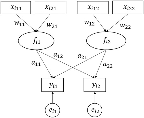
Each weight indicates how a predictor contributes to producing its corresponding component, which is in turn to explain outcome variables. The regression coefficients in A are another set of parameters, each of which indicates the effect of each component on an outcome variable.

Parameter estimation

The ordinary ERA model contains two sets of parameters to be estimated: component weights (W) and loadings (A). These unknown parameters are estimated by minimizing the following sum of squares (SS) objective function: (4) $$\varphi =\text{SS}\left(\mathbf{Y}-\mathbf{XWA}\right),$$(4) with respect to W and A, subject to the constraint $\mathit{diag}\left({\mathbf{F}}^{\mathbf{\prime }}\mathbf{F}\right)=N\mathbf{I}.$ An alternating least squares algorithm (ALS; de Leeuw et al. 1976) is developed to minimize the criterion (Takane & Hwang, 2005). The ALS algorithm repeats two main steps until convergence. In the first step, we update W for fixed A. The objective function (4) can be re-written as: (5) $$\begin{array}{c}\varphi =\text{SS}\left(\text{vec}\left(\mathbf{Y}\right)-\text{vec}\left(\mathbf{XWA}\right)\right)\\ =\text{SS}\left(\text{vec}\left(\mathbf{Y}\right)-\left({\mathbf{A}}^{\mathbf{\prime }}\otimes \mathbf{X}\right)\text{vec}\left(\mathbf{W}\right)\right),\end{array}$$(5) where $\otimes$ refers to the Kronecker product and $\text{vec}\left(\mathbf{W}\right)$ is the supervector formed by staking the columns of W. Let ${\mathbf{W}}^{*}$ denote a column vector formed by eliminating zero elements from $\text{vec}\left(\mathbf{W}\right),$ and $\mathbf{\Omega }$ denote a matrix formed by eliminating the columns of ${\mathbf{A}}^{\mathbf{\prime }}\otimes \mathbf{X}$ corresponding to the zero elements in $\text{vec}\left(\mathbf{W}\right).$ The least squares estimate of ${\mathbf{W}}^{*}$ is obtained as (6) $${\widehat{\mathbf{W}}}^{*}={\left({\mathbf{\Omega }}^{\mathbf{\prime }}\mathbf{\Omega }\right)}^{-1}{\mathbf{\Omega }}^{\mathbf{\prime }}\text{vec}\left(\mathbf{Y}\right).$$(6)

After reconstructing W from$\mathrm{}{\mathbf{W}}^{*},$ the updated W is multiplied by $\sqrt{N\text{inv}({\mathbf{W}}^{\mathbf{\prime }}{\mathbf{X}}^{\mathbf{\prime }}\mathbf{X}\mathbf{W})}$ to satisfy the constraint $\mathit{diag}\left({\mathbf{F}}^{\mathbf{\prime }}\mathbf{F}\right)=N\mathbf{I}.$

In the second step, we update A for fixed W. Minimizing (4) with respect to A is equivalent to minimizing: (7) $$\begin{array}{c}\varphi =\text{SS}\left(\text{vec}\left(\mathbf{Y}\right)-\text{vec}\left(\mathbf{XWA}\right)\right)\\ =\text{SS}\left(\text{vec}\left(\mathbf{Y}\right)-\left(\mathbf{I}\otimes \mathbf{F}\right)\text{vec}\left(\mathbf{A}\right)\right)\\ =\text{SS}\left(\text{vec}\left(\mathbf{Y}\right)-\mathbf{\Gamma }{\mathbf{A}}^{*}\right),\end{array}$$(7) where $\mathbf{\Gamma }$ is a matrix formed by removing the columns in $\left(\mathbf{I}\otimes \mathbf{F}\right)$ that correspond to zero elements in $\text{vec}\left(\mathbf{A}\right),$ and ${\mathbf{A}}^{*}$ is a column vector formed by eliminating zero elements from $\text{vec}\left(\mathbf{A}\right).$ The least squares estimate of ${\mathbf{A}}^{*}$ is given by (8) $${\widehat{\mathbf{A}}}^{*}={\left({\mathbf{\Gamma }}^{\mathbf{\prime }}\mathbf{\Gamma }\right)}^{-1}{\mathbf{\Gamma }}^{\mathbf{\prime }}\text{vec}\left(\mathbf{Y}\right).$$(8)

Similarly, A is then recovered from ${\mathbf{A}}^{*}.$

In this algorithm, the signs of the updated parameter estimates can change between iterations without changing their interpretations. For example, if a set of predictors is positively associated with its component (i.e., positive weights) and the component has positive effects on outcome variables (i.e., positive regression coefficients), the interpretation of these relationships still remains the same even if the signs of both the weights and regression coefficients become negative. This is in fact the same in BERA, which will be discussed in the next section. Typically, ERA imposes a sign constraint by either fixing the sign of each component on the basis of empirical/substantive meanings or determining the sign as the sign of the weight estimate that results in the strongest association with outcome variables.

Bayesian extended redundancy analysis

Bayesian analysis treats an unknown parameter as a random variable rather than fixed, and quantifies the uncertainty about the parameter using its probability distribution. The probabilistic statement about the parameter is inferred from updating the so-called posterior distribution, which is a combination of evidence collected from data that is formally expressed by the likelihood function and a prior belief that is specified with a prior distribution. Because the posterior distribution cannot be expressed as a closed form analytically, especially for multiple parameters, an MCMC algorithm is used to approximate the posterior distribution. For example, a Gibbs sampler is one of the most popular MCMC algorithms, which iteratively draws samples from relatively simpler full conditional distributions (Geman & Geman, 1984).

In ordinary ERA, there is an implicit assumption of independent residuals with zero means but no form of the likelihood since no error distribution is assumed. For BERA, however, we need to additionally consider a reasonable distribution for vector residuals, which can be a multivariate normal distribution such that (9) $${\mathbf{E}}_{[,q]}=(e_{1q},\dots ,e_{\mathit{Nq}}{)}^{\prime }\sim \mathit{MVN}(0,{\sigma }_q^2\mathbf{I}),$$(9) for q = 1, …, Q.

Conjugate priors

To make the posterior sampling process efficient, we consider conjugate prior distributions for the parameters. One reason for employing conjugate priors is that the posterior distribution can be derived as the same known family of the prior distribution, while still combining information from the prior and the data. Another reason is that with a large valued variance of the prior distribution, these conjugate priors become non-informative or diffuse priors with no concern of an improper posterior distribution. Last but not least, in a case where a non-conjugate prior is considered, the posterior distributions are known up to the normalizing constant and therefore a general Metropolis-Hastings algorithm (Hastings, 1970; Metropolis & Ulam, 1949) is implemented instead with some tuning parameter, which is difficult for a researcher with a minimal statistics background to control. With conjugate priors, all the full conditional distributions in a Gibbs sampler, as proposed in this article, are expressed as known distributions and therefore general audience can easily run the algorithm simply by specifying hyperparameters of the conjugate prior distributions.

Let W_[,k] denote a p_k by 1 column vector containing the weight estimates for the kth component, and A_[,q] denote a K by 1 column vector containing the regression coefficients affecting the qth outcome variable. In BERA, we consider the following conjugate priors: (10) $$\begin{array}{c}{\mathbf{W}}_{[,k]}|{\tau }^2\sim \mathit{MV}{N}_{p_k}\left(0,{\tau }^2\mathbf{I}\right)\text{for}k=1,...,K\\ {\tau }^2|a_1,b_1\sim \mathit{IG}\left(a_1,b_1\right)\\ {\mathbf{A}}_{[,q]}|{\sigma }_q^2\sim \mathit{MV}{N}_K\left(0,c_q{\sigma }_q^2\mathbf{I}\right)\text{for}q=1,...,Q\\ {\sigma }_q^2|a_0,b_0\sim \mathit{IG}\left(a_0,b_0\right)\text{for}q=1,...,Q,\end{array}$$(10) where a scalar constant $c_q$ ($c_q$ > 0) for the qth outcome variable is used to determine the dispersion of ${\mathbf{A}}_{[,q]}.$ If we set $c_q$ to large values such as $c_q$ = 100, the prior distribution on ${\mathbf{A}}_{[,q]}$ will become a diffuse prior conditional on ${\sigma }_q^2.$ Although we can fix ${\tau }^2$ and ${\sigma }_q^2$ to constant values to fully utilize the appealing features of Bayesian inference, we specify a hyperprior for ${\tau }^2$ and a prior for ${\sigma }_q^2.$ As one major objective of the paper is to introduce the general usage of BERA, a set of objective priors, that is, diffuse conjugate priors, (e.g., Chen, Bakshi, & Goel, 2009; Spiegelhalter, Thomas, Best, & Lunn, 2003) are specified with a₀ = b₀ = 1 and $c_q$ = 100 for simulated and real data analyses. Any subjective information obtained from previous research findings would also be formulated with power priors, as discussed in the next section.

Power priors

As the capability of incorporating any relevant prior information into a statistical analysis is one of the advantages of Bayesian methodologies, we consider using a power prior, that is, an informative prior constructed from historical data (Ibrahim & Chen, 2000; Ibrahim et al., 2015) for BERA. Because the accumulation of information occurs from past to future, it is natural to construct a prior from any previous research findings or information from historical data.

Following the notations of Ibrahim and Chen (2000), the power prior distribution for the current study can be expressed as (11) $$\pi \left(\theta |D_0,\delta \right)\propto L{\left(\theta |D_0\right)}^{\delta }{\pi }_0\left(\theta |c_0\right),$$(11) where $L\left(\theta |D_0\right)$indicates the likelihood for the historical data D₀ given a set of parameters $\theta ,$ and $\pi$₀($\theta$|$\cdot$) denotes the initial prior distribution for$\theta ,$ and $c_0$ is a specified hyperparameter for the initial prior. Note that the power parameter $\delta$ will serve as a weight that controls for the influence of the historical data on the current data, and it is reasonable to restrict the range of $\delta$ to be between 0 and 1, 0 $\le \mathrm{}\delta$$\mathrm{}\le$ 1. When $\delta$$\mathrm{}$= 0, no information from the historical data is incorporated (no borrowing), leading to the usual update through Bayes’ Theorem (or Bayes’ rule) only with the initial prior distribution. On the other hand, $\delta$$\mathrm{}$= 1 gives equal weights to $L\left(\theta |D_0\right)$ and the likelihood of the current data. In Ibrahim et al. (2015), power priors are extended to accommodate multiple historical datasets, imposing a power parameter ${\delta }_m$ for the mth historical data. With ${\delta }_m$ defined distinctively from past to near past, the priors from the historical data sets can accumulate information. Although we may update $\delta$ by modeling a hyperprior (e.g., a beta prior, a truncated gamma prior, or a truncated normal prior) as suggested by Ibrahim and Chen (2000), it might be more appealing to consider few possible values of $\delta$ based on the analytic meaning of the estimated weights and regression coefficients for interpretation purposes. This is common practice in applied research implementing a power prior (Rietbergen, Klugkist, Janssen, Moons, & Hoijtink, 2011; Shao 2012), which we also follow by evaluating how results would change depending on the values of $\delta$ as sensitivity analyses.

In this article, we only consider a power prior from the nearest past with the initial prior distribution for $\theta$ in (11) being an improper uniform prior, that is ${\pi }_0\left(\theta |c_0\right)\propto 1,$ for simplicity. Even though the proposed method can be extended with many sets of past studies, we consider a simple form of priors for comparisons to ordinary ERA. In BERA, power priors are specified as:

• Power Normal prior on W $${\mathbf{W}}_{[,k]}|{\mathbf{W}}_0{}_{[,k]},{\mathbf{\Sigma }}_{{\tau }_k}\sim {\left[\mathit{MV}{N}_{p_k}\left({\mathbf{W}}_0{}_{[,k]},{\mathbf{\Sigma }}_{{\tau }_k}\right)\right]}^{\delta },$$ where ${\mathbf{W}}_0{}_{[,k]}$ is a mean vector of weights from the past study for the kth component and ${\mathbf{\Sigma }}_{{\tau }_k}$ is a diagonal matrix with (${\tau }_1^2,...,{\tau }_{p_k}^2$), where ${\tau }_l^2$ is the variance of $w_{\mathit{lk}}.$ Although it is possible to further consider a hyperprior distribution (e.g., inverse Wishart priors) on ${\mathbf{\Sigma }}_{{\tau }_k},$ we fix them with the estimated values from the historical data.

• Power Normal prior on component loading A $${\mathbf{A}}_{[,q]}|{\mathbf{A}}_0{}_{[,q]},{\mathbf{\Sigma }}_{{\gamma }_q}\sim {\left[\mathit{MV}{N}_K\left({\mathbf{A}}_0{}_{[,q]},{\mathbf{\Sigma }}_{{\gamma }_q}\right)\right]}^{\delta },$$ where ${\mathbf{A}}_0{}_{[,q]}$ is the qth outcome variable’s mean vector of regression coefficients and ${\mathbf{\Sigma }}_{{\gamma }_k}$is a diagonal matrix with (${\gamma }_1^2,...,{\gamma }_K^2$) from the past study.

• An Inverse Gamma prior on ${\sigma }_q^2$ $${\sigma }_q^2|a_0,b_0\sim \mathit{IG}\left(a_0,b_0\right)$$ for q = 1, …, Q. For a simpler notation, let $\mathbf{\Sigma }=\mathit{diag}\left({\sigma }_1^2,...,{\sigma }_Q^2\right)$ hereinafter.

It is worthy to note two things related to the above formulation of power priors. First, it is common in practice to report maximum-likelihood estimates (MLEs) for parameters of interest and their standard errors, but not the estimated covariance matrix of the parameter estimates as a result of data analysis. Taking this practice into account together with the asymptotic normality of MLEs (Casella & Berger, 2002), it is natural to assume that both the prior variance matrices ${\mathbf{\Sigma }}_{{\tau }_k}$ and ${\mathbf{\Sigma }}_{{\gamma }_q}$of weight W_{[, k]} and regression coefficients ${\mathbf{A}}_{[,q]}$ in the conjugate multivariate normal prior distributions are to be a diagonal matrix with diagonal elements being squared standard errors of the corresponding parameter estimates from the past study. In a case where the full data set or the estimated covariance matrix of parameter estimates is available from the past study, the prior variance matrices can be specified to incorporate covariance information of the parameter estimates further. Second, because of the conjugacy of the above power priors, there will be no improper posterior issue even with power parameters.

Dealing with missing data in BERA

For simplicity, we assume that missingness occurs in outcome variables only, which is typically contemplated in a model with missing data (e.g., Asparouhov & Muthén, 2010). In this setting, it is reasonable to assume that missing data are classified as missing at random (MAR), that is, missing responses on an outcome variable can depend on predictors and other outcome variables but not on the outcome variable itself (Rubin, 1976, 1978). Missing completely at random (MCAR), that is, missing responses on an outcome variable is unrelated to any other variables, is another missing pattern that researchers in the social sciences typically assume (Schlomer et al., 2010). However, because MAR is a more general assumption than MCAR, we incorporate multiple imputation to handling missing data, which is known to hold well under the assumption of MAR.

In the presence of missing responses, the qth outcome variable vector ${\mathbf{Y}}_{[,q]}=(y_{1q},\dots ,y_{\mathit{Nq}}{)}^{\prime }$ can be written as Y_[,q] = (Y_obs[,q], Y_mis[,q]), where Y_obs and Y_mis are vectors of observed and missing responses, respectively. Let $\mathbf{\Theta }=\{\mathbf{W},\mathbf{A},{\sigma }_1^2,\dots {\sigma }_Q^2\}$ denote a set of all parameters. Then, the likelihood function of $\mathbf{\Theta }$ and Y_mis, given Y_obs, can be written as (12) $$L\left(\mathbf{\Theta },{\mathbf{Y}}_{\text{mis}}|{\mathbf{Y}}_{\text{obs}}\right)=L\left(\mathbf{\Theta }|{\mathbf{Y}}_{\text{obs}}\right)L\left({\mathbf{Y}}_{\text{mis}}|\mathbf{\Theta },{\mathbf{Y}}_{\text{obs}}\right).$$(12)

Based on (10), we implement a Bayesian approach to multiple imputation by generating a Markov chain that iterates the imputation and posterior sampling steps as follows. At the (s + 1)th iteration,

• Imputation step: ${\mathbf{Y}}_{\text{mis}}^{(s+1)}\sim \pi \left({\mathbf{Y}}_{\text{mis}}|{\mathbf{Y}}_{\text{obs}},{\mathbf{\Theta }}^{(s)}\right)$

• Posterior sampling step: ${\mathbf{\Theta }}^{(s+1)}\sim \pi \left(\mathbf{\Theta }|{\mathbf{Y}}_{\text{obs}},{\mathbf{Y}}_{\text{mis}}^{(s+1)}\right).$

The imputation step generates new samples from the conditional distribution of Y_mis, given Y_obs and the current values of the parameters. Then, using the just updated values of Y_mis, each set of the parameters is sampled from the posterior distribution based on full-data likelihood $\pi \left(\mathbf{\Theta }|{\mathbf{Y}}_{\text{obs}},{\mathbf{Y}}_{\text{mis}}^{(s+1)}\right).$ The imputation step above is a data augmentation (Tanner & Wong, 1987; Schafer, 1997; van Dyk & Meng, 2001), which enables full-data inference even in the presence of missing responses.

In BERA, the full conditional distribution of Y_mis[,q], given all the other parameters $\mathbf{\Theta }$ in the imputation step, is obtained from a multivariate normal distribution as (13) $${\mathbf{Y}}_{\text{mis}[,q]}|\mathbf{W},\mathbf{A},{\sigma }_1^2,\dots ,{\sigma }_Q^2,{\tau }^2,\mathbf{X},{\mathbf{Y}}_{\text{obs}[,q]}\sim \mathit{MVN}\left(\underset{\_}{\mathbf{X}}\mathbf{W}{\mathbf{A}}_{[,q]},{\sigma }_q^2\mathbf{I}\right),$$(13) where N* is the number of observed responses for the qth outcome variable, $\underset{\_}{\mathbf{X}}$ is an (N - N*) by P matrix of predictors, and I is the identity matrix of order (N - N*). Then, the posterior sampling step is carried out using the Gibbs sampling with either conjugate or power priors, as discussed earlier. Further details on the sampling scheme with the full conditional distributions are provided in the Appendix.

Other computational issues in BERA

As the same scale indeterminacy between F and A remains in BERA, we impose the same scaling constraint of $\mathit{diag}\left({\mathbf{F}}^{\mathbf{\prime }}\mathbf{F}\right)=N\mathbf{I}$ on each component. Also in BERA, to avoid the potential sign-switching between W and A, we fix signs of W to the sign of a weight estimate that yields the strongest association with outcome variables.

To examine if a sequence of posterior samples obtained from an MCMC method converges to the target distribution after a number of iterations, we check convergence and mixing of a chain by drawing trace plots for the samples simulated. When a lack of convergence and mixing is suspected by showing a systematic or cyclic trend over the iterations (e.g., staying in a certain range of values for a longer period of time rather than traversing up and down), we would increase the number of early iterations to discard in the chain (i.e., a burn-in period) (Lynch, 2007) and/or choose every rth posterior sample (i.e., a thinning) to improve the mixing of the chain. To monitor dependency among posterior samples and determine the value of r in the thinning, autocorrelation function (ACF) plots are used to check around what lag the autocorrelations decrease to being not significantly different from zero (decrease towards zero). Additionally, we also check convergence of the proposed MCMC algorithm by running chains multiple times with different initial values for parameters.

Examples

Simulation studies

We conducted two series of simulations studies to investigate how well the proposed method performed in terms of recovering the original underlying structure of the data under different conditions. Across the different conditions, the number of predictors, components, and outcome variables remained the same as shown in Figure 1: Q = 2, K = 2, and $p_k$ = 2 for k = 1 and 2. The weight and regression coefficient parameters in W and A in (2) were prescribed as $$\mathbf{W}=\left[\begin{array}{cc}0.9& 0\\ 0.5& 0\\ 0& 0.5\\ 0& 0.5\end{array}\right]\text{and}\mathbf{A}=\left[\begin{array}{cc}2& 1\\ 1.5& 1.5\end{array}\right].$$

Furthermore, X and Y in (2) were assumed to be generated from $$\mathbf{X}\sim \mathit{MV}{N}_P\left(0,\mathbf{\Omega }\right)\text{and}\mathbf{Y}\sim \mathit{MV}{N}_Q\left(0,\mathbf{\Sigma }\right),$$

where $\mathbf{\Omega }=\left[\begin{array}{cccc}1& 0.3& 0.1& 0.1\\ 0.3& 1& 0.1& 0.1\\ 0.1& 0.1& 1& 0.3\\ 0.1& 0.1& 0.3& 1\end{array}\right]$and $\mathbf{\Sigma }=\left[\begin{array}{cc}1.2& 0.1\\ 0.1& 0.8\end{array}\right].$

A summary of other model specifications varied at each condition is provided as follows:

• Condition 1: We set the two outcome variables to be continuous without missing values. Four different sample sizes were considered: N = 50, 100, 200, and 1000.

• Condition 2: The data were generated in the same way as in Condition 1 across the sample sizes, except that the proportion of missingness in the outcome variables was also varied. We considered two levels of the proportions of missingness, that is, 30% and 50% of the responses in an outcome variable were set to be missing. Three combinations of these two proportions were then considered for two outcome variables: 30–30%, 30–50%, and 50–50%. Note that the sample size of N = 50 was not considered in this condition, because the combination of 50–50% missingness may result in a too small sample size, which in turn would not be advisable to carry out ordinary ERA with a complete-case analysis.

To analyze simulated data in absence of relevant prior research findings or belief, diffuse conjugate prior distributions were considered first (i.e., without power prior specifications, $\delta$$\mathrm{\hspace{0.17em}}$= 0). In specific, we assigned the conjugate priors as specified in (10) with a hyperprior for ${\tau }^2$ set to follow an inverse-gamma distribution ${\tau }^2\sim \mathit{IG}\left(1,1\right),$ $c_q$= 100 for q = 1, …, Q, and a₀ = b₀ = 1. These specifications were set to ensure a large variance and thus diffuse priors on the parameters of interest. This makes the contribution of the priors the least, while allowing for the comparison with the ordinary ERA.

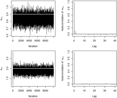
Both BERA and the ordinary ERA were applied to the simulated data to compare their recovery of the parameters of interest. Moreover, BERA was applied with and without imputation for Condition 2 to compare their relative performance of multiple imputation. For BERA, the total number of iterations were set at 10,000. Fast convergence and good mixing of the MCMC chain was observed for all parameters of interest across all the simulation scenarios considered and the autocorrelations of the posterior samples were kept <0.01 after the lag time of 3 or more (Figure 2). Based on these observations, the first 1000 iterations were discarded as a burn-in period and every fifth posterior sample was used by applying a thinning approach to calculate the posterior means, standard deviations, and HPD credible intervals (CI) of parameters of interest. For ordinary ERA, the bootstrap method (Efron, 1982), with 500 bootstrap samples, was used to obtain the 95% percentile bootstrap confidence intervals of parameter estimates.

Figure 2. Trace and autocorrelation function (ACF) plots of weight element w₁₁ (top row) and regression coefficient a₁₁ (bottom row) in Condition 1 with N = 50. The white horizontal solid line in the trace plot indicates the true value.

Table 1 presents the results of analyzing the simulated data under Condition 1. As the sample size increased, posterior mean estimates obtained from BERA became closer to the parameters on average. The posterior standard deviations as well as the width of the credible intervals decreased with the sample size, as expected. This was the case for the bootstrapped confidence intervals obtained from ERA. The similarity between the results of BERA and ERA was not entirely surprising given that the Bayesian estimates here were obtained using diffuse prior distributions. Nevertheless, at a relatively small sample size (N = 100), the width of the bootstrapped confidence intervals from ERA tended to be wider than that of the credible intervals from BERA. This difference in the interval’s width decreased with the sample size. Overall, BERA seemed to recover the prescribed parameters sufficiently well.

Table 1. Results of the simulation study under Condition 1 applying BERA (with diffuse priors) and ordinary ERA.

		BERA				ERA
	truth	post.mean	post.sd	95CI.low	95CI.up	est.	bCI.low	bCI.up
	N = 50
w11	0.9	0.841	0.056	0.724	0.944	0.818	0.676	1.085
w21	0.5	0.481	0.067	0.354	0.615	0.495	0.374	0.667
w12	0.5	0.414	0.055	0.309	0.521	0.428	0.304	0.606
w22	0.5	0.566	0.047	0.473	0.656	0.546	0.402	0.722
a11	2	1.887	0.130	1.648	2.147	1.852	1.429	2.241
a12	1.5	1.528	0.184	1.142	1.884	1.611	1.103	2.114
a21	1	1.163	0.108	0.946	1.372	1.135	0.719	1.533
a22	1.5	1.724	0.151	1.432	2.039	1.795	1.317	2.180
	N = 100
w11	0.9	0.832	0.035	0.761	0.898	0.831	0.711	1.004
w21	0.5	0.522	0.042	0.440	0.604	0.517	0.426	0.643
w12	0.5	0.544	0.034	0.478	0.609	0.542	0.463	0.645
w22	0.5	0.494	0.036	0.420	0.560	0.492	0.390	0.599
a11	2	2.090	0.083	1.933	2.263	2.057	1.698	2.423
a12	1.5	1.470	0.118	1.247	1.717	1.510	1.126	1.866
a21	1	0.871	0.080	0.704	1.017	0.866	0.644	1.064
a22	1.5	1.444	0.112	1.239	1.674	1.488	1.207	1.781
	N = 200
w11	0.9	0.889	0.024	0.843	0.935	0.885	0.783	0.937
w21	0.5	0.467	0.032	0.406	0.528	0.468	0.390	0.561
w12	0.5	0.488	0.028	0.435	0.541	0.487	0.420	0.564
w22	0.5	0.527	0.026	0.474	0.576	0.527	0.460	0.611
a11	2	2.010	0.067	1.871	2.127	1.967	1.769	2.193
a12	1.5	1.495	0.099	1.318	1.695	1.528	1.287	1.758
a21	1	0.961	0.053	0.854	1.059	0.939	0.812	1.078
a22	1.5	1.439	0.078	1.284	1.592	1.471	1.245	1.694
	N =1000
w11	0.9	0.897	0.010	0.879	0.916	0.897	0.854	0.940
w21	0.5	0.505	0.013	0.480	0.530	0.504	0.472	0.504
w12	0.5	0.520	0.012	0.497	0.544	0.519	0.486	0.556
w22	0.5	0.493	0.012	0.470	0.518	0.494	0.464	0.528
a11	2	2.061	0.027	2.010	2.115	2.017	1.914	2.117
a12	1.5	1.447	0.039	1.366	1.519	1.459	1.357	1.553
a21	1	0.993	0.025	0.944	1.043	0.971	0.904	1.035
a22	1.5	1.459	0.035	1.389	1.531	1.473	1.383	1.571

Note: post.mean = posterior mean; post.sd = posterior standard deviation; CI.low = lower bound of the 95% HPD credible interval; CI.up = upper bound of the 95% HPD credible interval; est. = mean parameter estimate; bCI.low = lower bound of the bootstrapped 95% confidence interval; bCI.up = upper bound of the bootstrapped 95% confidence interval. These abbreviated terms remained the same hereinafter.

In addition to the analysis of data from Condition 1 with diffuse priors, we applied power prior distributions to the same condition in order to examine whether the results obtained from BERA were sensitive to different prior specifications. For this, an independent set of samples was generated from the same simulation model with a sample size of 50 and used as historical data, whose obtained posterior means and standard deviations served as the hyperparameter values for specifying the power prior distributions. By fixing the sample size of historical data as N = 50 across the four different sample sizes in Condition 1, we would also investigate how the amount of information in the likelihood overwhelms that in the prior. Table 2 presents results of Condition 1 with the informative prior distributions while varying across three different values of the power parameter ($\delta$ = 0.2, 0.34, and 0.5). Results obtained under N = 1000 is provided in the Supplemental materials (refer to Supporting Information Table S1) to improve readability of Table 2. Note that the last two rows in the table are the results of the historical data itself with N = 50, which were used as hyperparameters in power priors. Overall, on average, the posterior mean estimates after updating the power prior regardless of the power parameter $\delta$ were closer to the true parameters, and their posterior standard deviations and their HPD intervals were smaller and narrower, respectively, compared to the results with the same sample size in Table 1 (Condition1 with diffuse priors). These were shown consistently regardless of different degrees of the power parameter $\delta .$ The accuracy of recovering the true parameter values increased with a better precision as the sample size of current data from Condition 1 increased. In case of analyzing larger sample sizes of current data (e.g., N ≥ 100), it was observed that the posterior was mainly dominated by the likelihood. Because of the small sample size used in the historical data, some estimated parameters were found to be notably deviated from the true parameter value (e.g., the mean of w₁₂ was estimated as 0.337 when its true value was 0.5). When the current data have sufficient number of sample sizes, however, we rather observed stable results, recovering the true values well. This suggested that even with a power prior distribution specified with a less accurate hyperparameter value, BERA would be still able to produce robust results if there are sufficient number of sample size in current data.

Table 2. Results of the simulation study under Condition 1 applying BERA with informative power priors varying the power parameters (δ = 0.2, 0.34, and 0.5).

		N = 50				N = 100				N = 200
	truth	post.mean	post.sd	95CI.low	95CI.up	post.mean	post.sd	95CI.low	95CI.up	post.mean	post.sd	95CI.low	95CI.up
						$\delta$ = 0.2
w11	0.9	0.972	0.029	0.916	1.031	0.963	0.025	0.914	1.010	0.914	0.019	0.878	0.953
w21	0.5	0.419	0.046	0.328	0.510	0.458	0.039	0.382	0.531	0.490	0.027	0.435	0.541
w12	0.5	0.513	0.040	0.427	0.585	0.517	0.037	0.446	0.592	0.489	0.027	0.431	0.536
w22	0.5	0.500	0.041	0.423	0.582	0.514	0.037	0.443	0.588	0.508	0.026	0.459	0.562
a11	2	2.219	0.110	2.001	2.442	1.904	0.085	1.735	2.067	2.089	0.063	1.968	2.217
a12	1.5	1.684	0.162	1.361	1.985	1.268	0.123	1.024	1.507	1.412	0.091	1.218	1.578
a21	1	1.056	0.103	0.849	1.247	0.985	0.077	0.842	1.148	0.891	0.053	0.780	0.992
a22	1.5	1.711	0.140	1.443	1.981	1.504	0.107	1.299	1.711	1.504	0.073	1.357	1.646
						$\delta$ = 0.34
w11	0.9	0.976	0.026	0.926	1.030	0.971	0.023	0.928	1.015	0.923	0.018	0.890	0.960
w21	0.5	0.413	0.042	0.325	0.490	0.446	0.036	0.372	0.512	0.479	0.026	0.426	0.527
w12	0.5	0.506	0.037	0.429	0.576	0.511	0.035	0.446	0.582	0.486	0.026	0.436	0.538
w22	0.5	0.508	0.037	0.436	0.583	0.519	0.034	0.456	0.592	0.510	0.025	0.464	0.563
a11	2	2.210	0.103	1.999	2.411	1.922	0.082	1.767	2.086	2.091	0.062	1.972	2.215
a12	1.5	1.641	0.152	1.331	1.917	1.272	0.118	1.035	1.499	1.411	0.089	1.221	1.572
a21	1	1.043	0.096	0.852	1.222	0.981	0.074	0.844	1.137	0.891	0.052	0.783	0.990
a22	1.5	1.714	0.130	1.466	1.967	1.522	0.103	1.317	1.711	1.513	0.072	1.371	1.653
						$\delta$ = 0.5
w11	0.9	0.979	0.024	0.933	1.028	0.977	0.021	0.937	1.017	0.930	0.017	0.897	0.964
w21	0.5	0.409	0.038	0.328	0.479	0.436	0.034	0.369	0.499	0.469	0.025	0.418	0.515
w12	0.5	0.500	0.035	0.431	0.568	0.507	0.033	0.445	0.574	0.484	0.025	0.436	0.534
w22	0.5	0.514	0.034	0.447	0.582	0.524	0.032	0.465	0.591	0.512	0.024	0.469	0.564
a11	2	2.202	0.096	2.019	2.402	1.940	0.079	1.792	2.097	2.092	0.060	1.977	2.213
a12	1.5	1.604	0.143	1.313	1.864	1.277	0.113	1.042	1.484	1.409	0.087	1.221	1.564
a21	1	1.032	0.090	0.854	1.201	0.978	0.071	0.848	1.129	0.892	0.051	0.785	0.988
a22	1.5	1.717	0.121	1.488	1.954	1.540	0.098	1.348	1.725	1.523	0.070	1.383	1.660

Table

Summary of the historical data (N = 50)
		w11	w21	w12	w22	a11	a12	a21	a22
	post.mean	0.879	0.337	0.549	0.648	2.466	1.094	1.103	1.398
	post.sd	0.024	0.042	0.063	0.059	0.124	0.126	0.114	0.112

Tables 3 and 4 show the results under Condition 2 across different sample sizes. Results with the sample size of N = 1000 are presented in the Supplemental materials at Supporting Information Table S2. The number of complete cases was reported as N* in the corresponding combination of missingness on the outcome variables. For example, at N = 100, there were 22 cases left after removing those containing missing responses (N* = 22). The width of the credible interval tended to become wider as the proportion of missingness increased. This pattern was observed regardless of the sample sizes. BERA with imputation outperformed the other two alternative methods, that is, BERA without imputation and ordinary ERA, across all possible levels of missingness and sample sizes. When the total sample size was not large enough (e.g., N = 100) and N* was less than half of N, the estimates from BERA without imputation and ordinary ERA were less accurate with wider credible/confidence intervals. Thus, when missing responses are present, it can be more useful to apply BERA with imputation, particularly when N* was less than half of N.

Table 3. Results of the simulation study under Condition 2 with N = 100 (N* indicates the number of complete-case sample sizes).

	BERA with imputation					BERA without imputation				ERA
	truth	post.mean	post.sd	95CI.low	95CI.up	post.mean	post.sd	95CI.low	95CI.up	est	95CI.low	95CI.up
	30-30 missing					N* = 48
w11	0.9	0.833	0.043	0.743	0.909	0.793	0.054	0.681	0.899	0.790	0.652	1.024
w21	0.5	0.520	0.052	0.427	0.625	0.499	0.053	0.399	0.611	0.490	0.348	0.662
w12	0.5	0.538	0.039	0.461	0.610	0.534	0.045	0.449	0.625	0.529	0.410	0.694
w22	0.5	0.500	0.041	0.419	0.575	0.504	0.050	0.410	0.602	0.504	0.404	0.650
a11	2	2.066	0.100	1.858	2.248	2.145	0.130	1.887	2.413	2.113	1.598	2.609
a12	1.5	1.555	0.146	1.266	1.836	1.630	0.187	1.278	1.994	1.684	1.140	2.198
a21	1	0.890	0.097	0.698	1.086	0.975	0.117	0.752	1.212	0.951	0.650	1.214
a22	1.5	1.479	0.141	1.214	1.752	1.320	0.171	0.977	1.644	1.374	1.028	1.732
	30-50 missing					N* = 36
w11	0.9	0.843	0.042	0.766	0.929	0.758	0.059	0.643	0.868	0.758	0.626	0.980
w21	0.5	0.508	0.052	0.409	0.609	0.513	0.059	0.398	0.623	0.516	0.362	0.716
w12	0.5	0.540	0.041	0.459	0.616	0.536	0.053	0.437	0.640	0.531	0.391	0.806
w22	0.5	0.498	0.043	0.414	0.580	0.514	0.055	0.408	0.619	0.528	0.414	0.716
a11	2	2.068	0.101	1.873	2.264	2.121	0.144	1.846	2.399	2.101	1.556	2.650
a12	1.5	1.556	0.145	1.268	1.828	1.587	0.204	1.171	1.993	1.643	1.108	2.236
a21	1	0.914	0.111	0.695	1.124	0.975	0.129	0.721	1.228	0.973	0.642	1.277
a22	1.5	1.366	0.151	1.061	1.674	1.137	0.182	0.757	1.480	1.177	0.847	1.530
	50-50 missing					N* = 22
w11	0.9	0.824	0.048	0.722	0.908	0.801	0.059	0.682	0.909	0.845	0.636	1.260
w21	0.5	0.531	0.057	0.427	0.646	0.345	0.094	0.159	0.521	0.351	0.128	0.783
w12	0.5	0.536	0.049	0.439	0.627	0.572	0.114	0.353	0.790	0.608	0.181	0.988
w22	0.5	0.501	0.051	0.400	0.596	0.556	0.149	0.264	0.839	0.607	0.328	1.023
a11	2	2.057	0.107	1.840	2.258	2.305	0.210	1.871	2.686	2.208	1.260	3.100
a12	1.5	1.514	0.182	1.183	1.882	1.022	0.312	0.384	1.612	1.534	0.674	2.284
a21	1	0.885	0.128	0.627	1.134	1.080	0.169	0.736	1.409	0.988	0.510	1.455
a22	1.5	1.455	0.168	1.117	1.769	0.834	0.253	0.275	1.288	1.092	0.027	1.668

Table 4. Results of the simulation study under Condition 2 with N = 200 (N* indicates the number of complete-case sample sizes)

	BERA with imputation					BERA without imputation				ERA
	truth	post.mean	post.sd	95CI.low	95CI.up	post.mean	post.sd	95CI.low	95CI.up	est	95CI.low	95CI.up
	30-30 missing					N* = 101
w11	0.9	0.888	0.032	0.827	0.950	0.800	0.036	0.732	0.873	0.797	0.662	0.952
w21	0.5	0.468	0.041	0.384	0.545	0.461	0.046	0.363	0.546	0.470	0.373	0.600
w12	0.5	0.490	0.035	0.419	0.554	0.514	0.047	0.418	0.604	0.517	0.393	0.660
w22	0.5	0.525	0.033	0.467	0.596	0.515	0.055	0.418	0.633	0.512	0.375	0.650
a11	2	1.988	0.083	1.828	2.155	2.163	0.103	1.958	2.362	2.131	1.773	2.448
a12	1.5	1.479	0.117	1.239	1.704	1.383	0.151	1.085	1.674	1.401	1.021	1.704
a21	1	0.943	0.063	0.818	1.060	1.050	0.086	0.882	1.208	1.033	0.833	1.234
a22	1.5	1.396	0.102	1.195	1.584	1.285	0.120	1.049	1.523	1.307	1.016	1.575
	30-50 missing					N* = 70
w11	0.9	0.874	0.034	0.810	0.940	0.832	0.044	0.750	0.921	0.833	0.682	1.054
w21	0.5	0.486	0.043	0.401	0.568	0.494	0.051	0.394	0.592	0.510	0.387	0.692
w12	0.5	0.481	0.037	0.407	0.551	0.569	0.055	0.459	0.676	0.567	0.424	0.733
w22	0.5	0.533	0.035	0.463	0.599	0.486	0.068	0.353	0.621	0.484	0.326	0.677
a11	2	1.989	0.082	1.823	2.141	2.099	0.122	1.864	2.339	2.071	1.671	2.443
a12	1.5	1.488	0.118	1.263	1.721	1.246	0.172	0.901	1.584	1.278	0.848	1.684
a21	1	0.949	0.070	0.818	1.096	1.004	0.093	0.821	1.179	0.999	0.757	1.249
a22	1.5	1.345	0.111	1.138	1.574	1.198	0.129	0.933	1.437	1.222	0.835	1.579
	50-50 missing								N* = 53
w11	0.9	0.909	0.036	0.842	0.981	1.028	0.050	0.925	1.118	0.833	0.801	1.234
w21	0.5	0.439	0.049	0.338	0.528	0.344	0.084	0.181	0.502	0.510	0.216	0.601
w12	0.5	0.505	0.038	0.431	0.581	0.450	0.052	0.352	0.555	0.567	0.327	0.670
w22	0.5	0.509	0.038	0.441	0.590	0.507	0.056	0.396	0.615	0.484	0.321	0.669
a11	2	1.980	0.110	1.756	2.189	1.815	0.140	1.558	2.092	2.071	1.340	2.135
a12	1.5	1.522	0.146	1.215	1.781	1.655	0.207	1.242	2.062	1.278	1.221	2.316
a21	1	0.899	0.072	0.757	1.032	0.772	0.115	0.556	1.003	0.999	0.462	1.007
a22	1.5	1.423	0.098	1.236	1.617	1.511	0.160	1.204	1.821	1.222	1.100	2.067

To further assess the properties of parameter estimates and investigate the relative performance of BERA with imputation, as compared to BERA without imputation and ordinary ERA, we replicated 1000 data sets at each scenario of Condition 2 and implemented all three methods. The biases and root mean square errors (RMSE) of the estimates of the parameters were calculated from each method. Table 5 displays the results with 1000 replicated data sets when the two proportions of missingness for two outcome variables were 50% each. As shown in the table, the magnitudes of biases and RMSE decreased with increasing sample sizes regardless of the methods. Nonetheless, it was noteworthy that the biases and RMSE estimated from BERA with imputation were always the smallest, indicating that it overall outperformed the alternative methods in recovering the true parameters. The biases obtained from BERA with imputation were quite close to zeros across all sample sizes, whereas those from the alternative methods were somewhat larger when N = 100. Similarly, the RMSE of BERA with imputation were about twice smaller than those of BERA without imputation and ordinary ERA consistently across different sample sizes. As expected, similar overall patterns of the biases and RMSE were observed for Condition 2 with the missing proportions of 30% - 30% combination, which is presented in Table S3 in the Supporting Information.

Table 5. The biases and root mean square errors (RMSE) of the 1000 simulation replicates with 50–50% of missingness across different sample sizes.

	BERA with imputation		BERA without imputation*		ERA*
	bias	RMSE	bias	RMSE	bias	RMSE
N = 50	0.010	0.081	0.035	0.223	0.045	0.257
	0.004	0.101	0.008	0.203	0.028	0.212
	−0.001	0.095	0.014	0.174	0.016	0.213
	−0.001	0.090	−0.071	0.223	0.013	0.197
	−0.028	0.219	−0.051	0.458	−0.036	0.447
	−0.015	0.283	−0.127	0.618	0.000	0.498
	−0.020	0.188	−0.023	0.312	−0.033	0.316
	−0.007	0.265	−0.129	0.573	−0.026	0.442
N = 100	0.001	0.054	0.024	0.153	0.029	0.150
	0.003	0.064	0.012	0.127	0.008	0.124
	0.000	0.059	0.010	0.117	0.017	0.128
	0.001	0.060	0.005	0.113	0.009	0.120
	−0.017	0.144	−0.037	0.313	−0.019	0.313
	−0.004	0.192	−0.006	0.340	−0.013	0.331
	−0.005	0.117	−0.014	0.208	−0.009	0.202
	−0.014	0.176	−0.031	0.309	−0.017	0.319
N = 200	0.001	0.039	0.011	0.097	0.013	0.095
	0.002	0.046	0.003	0.082	0.011	0.082
	−0.002	0.043	0.005	0.080	0.009	0.077
	0.002	0.043	0.005	0.077	0.005	0.075
	−0.007	0.097	−0.010	0.220	−0.018	0.213
	−0.006	0.138	−0.011	0.225	−0.002	0.227
	−0.005	0.082	−0.005	0.145	−0.009	0.144
	−0.005	0.124	−0.007	0.212	−0.006	0.210
N = 1000	0.000	0.017	0.000	0.042	0.002	0.042
	0.001	0.019	0.002	0.037	−0.002	0.034
	−0.001	0.018	0.001	0.034	0.001	0.032
	0.001	0.018	0.001	0.034	0.000	0.033
	−0.003	0.044	0.002	0.097	0.003	0.094
	−0.003	0.060	−0.003	0.103	0.001	0.098
	−0.001	0.037	−0.002	0.065	0.003	0.065
	−0.001	0.054	−0.002	0.101	0.004	0.096

*An average sample size for BERA without imputation and ERA across 1000 replicates was half of the corresponding sample size (N) for BERA with imputation due to 50% of missingness.

A real data example

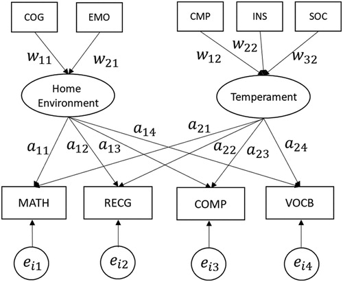
This section provides an example of applying BERA to analyze real data. The data used here were a subset of the National Longitudinal Survey of Youth 1979-Children (NLSY79-C) data (Center for Human Resource Research, 2000), where 440 children (N = 440) responded to nine observed variables in 2000. As displayed in Figure 3, five of the observed variables were predictors, including: (1) cognitive stimulation (COG), (2) emotional support (EMO), (3) compliance (CMP), (4) insecure attachment (INS), and (5) sociability (SOC). The component home environment was constructed as a linear combination of COG and EMO, measured using the Home Observation for Measurement of the Environment (Bradley & Caldwell, 1984). Another component temperament was defined as a linear combination of CMP, INS, and SOC, which were measured by Rothbart’s Infant Behavior Questionnaire (Rothbart, 1981) and Campos and Kagan’s Compliance Scale (Campos Joseph, Barrett, Lamb, Goldsmith, & Stenberg, 1983). The remaining four observed variables were outcome variables that assessed the performance of the children in mathematics (MATH), reading recognition (RECG), reading comprehension (COMP), and vocabulary (VOCB), using the Peabody Individual Achievement Test battery (Dunn & Markwardt, 1970) as well as the revised edition of the Peabody Picture Vocabulary Test (Dunn & Dunn, 1981). We assumed that each of the two components affected the outcome variables.

Figure 3. A model specification for the real data example.

Although the sample size was 440, only three children had responded to all of the four outcome variables, whereas the remaining participants had not responded to at least one of the outcome variables. If we excluded all cases having missing responses in any of the outcome variables, there would be only three cases left, which would be too small to apply ordinary ERA. Hence, we applied BERA with multiple imputation to the data.

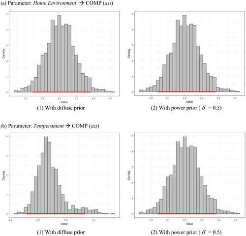
The MCMC algorithm converged fast and the mixing looked good (Supporting Information Figure S1). Therefore, in the analysis, the first 2000 iterations were discarded as a burn-in period, after which another set of 8000 iterations were run while saving posterior samples at every fifth iteration from the algorithm for the posterior inferences (i.e., setting the thinning interval = 5). As a summary of the posterior distribution, the posterior mean estimate and standard deviation, and the 95% HPD credible interval were calculated. Figure 4 presents two sets of exemplary posterior densities with their corresponding HPD intervals to make the figure concise. The model fit was satisfactory, since there were no notable patterns observed in residual plots (refer to Supporting Information Figure S2 in the Supplemental materials).

Figure 4. Density plots with highest posterior density (HPD) intervals, comparing posterior estimates results with diffuse and power priors: (a) displays the plots for the posterior regression coefficient estimates of Home Environment on COMP; and (b) displays the plots for regression coefficient estimates of Temperament on COMP. A red colored bar in each plot refers to its HPD interval.

Table 6 summarizes the results of the posterior distributions for the model parameters with the same diffuse priors specified in the simulation study. As expected, children who received more cognitive simulation (COG) and emotional support (EMO) were positively and statistically significantly associated with home environment, indicating that higher levels of COG (w₁₁ = 1.025, 95%CI = [0.916 1.133]) and EMO (w₂₁ = 0.246, 95%CI = [0.043 0.447]) led to higher scores of home environment. Both predictors contributed well to determining home environment, although the magnitude of COG was larger. With a 95% probability, the weight of COG on defining home environment lies between 0.916 and 1.133, and that of EMO resides between 0.043 and 0.447. On the other hand, insecure attachment (INS) more strongly contributed to constructing temperament than compliance (CMP) and children’s sociability (SOC). INS was also positively and statistically significantly associated with this component (w₄₂ = 0.333, 95%CI = [0.021 0.690]), whereas both CMP and SOC were not statistically significantly related to it. The component home environment had positive and statistically significant effects on all the four outcome variables (a₁₁ = 0.336, 95%CI = [0.225 0.433]; a₁₂ = 0.240, 95%CI = [0.140 0.351]; a₁₃ = 0.205, 95%CI = [0.043 0.385]; and a₁₄ = 0.409, 95%CI = [0.280 0.532]), suggesting that children’s home environment built on both cognitive simulation and emotional support were likely related to their competency on the different performance measures. In contrast, Temperament had no statistically significant impact on all the four outcome variables. This indicates that children’s academic achievements were not strongly related to their temperament that was dominantly determined by how much of the insecure attachment were formed in childhood.

Table 6. Results obtained from BERA with multiple imputation for the National Longitudinal Survey of Youth 1979-Children (NLSY79-C) data in 2000.

parameters	post.mean	post.sd	95CI.low	95CI.up
COG → Home Environment (w11)	1.025	0.057	0.916	1.133
EMO → Home Environment (w21)	0.246	0.106	0.043	0.447
CMP → Temperament (w12)	0.090	0.342	−0.556	0.759
INS → Temperament (w22)	0.333	0.184	0.021	0.690
SOC → Temperament (w32)	−0.727	0.501	−0.994	0.954
Home Environment → MATH (a11)	0.336	0.054	0.225	0.433
Home Environment → RECG (a12)	0.240	0.056	0.140	0.351
Home Environment → COMP (a13)	0.205	0.088	0. 043	0.385
Home Environment → VOCB (a14)	0.409	0.063	0.280	0.532
Temperament → MATH (a21)	−0.070	0.071	−0.193	0.133
Temperament → RECG (a22)	−0.164	0.121	−0.301	0.257
Temperament → COMP (a23)	−0.172	0.150	−0.414	0.305
Temperament → VOCB (a24)	−0.070	0.092	−0.239	0.165

For illustration, we analyzed another subset of the NLSY79-C data collected in an earlier year (i.e., year 1996) so as to use the findings for constructing power prior distributions. This data in 1996 consisted of 902 children who were completely independent of the 440 children measured in 2000. Table 7 represents the results of the data in 1996 using diffuse or uninformative prior distributions (i.e., the same prior distributions specified in the simulation study). Then, the results in Table 7 were used for constructing informative power prior distributions; the estimated posterior means and standard deviations of W and A were set as the hyperparemter values of the corresponding prior distributions in analyzing year 2000s data.

Table 7. Results obtained from BERA with multiple imputation for the National Longitudinal Survey of Youth 1979-Children (NLSY79-C) data in 1996.*

parameters	post.mean	post.sd	95CI.low	95CI.up
COG → Home Environment (w11)	1.005	0.049	0.908	1.092
EMO → Home Environment (w21)	0.219	0.089	0.057	0.388
CMP → Temperament (w12)	−0.376	0.112	−0.595	−0.147
INS → Temperament (w22)	0.696	0.094	0.515	0.870
SOC → Temperament (w32)	−0.555	0.106	−0.752	−0.358
Home Environment → MATH (a11)	0.307	0.038	0.232	0.379
Home Environment → RECG (a12)	0.274	0.039	0.202	0.350
Home Environment → COMP (a13)	0.152	0.083	−0.012	0.340
Home Environment → VOCB (a14)	0.345	0.052	0.240	0.439
Temperament → MATH (a21)	−0.177	0.039	−0.252	−0.099
Temperament → RECG (a22)	−0.173	0.040	−0.252	−0.100
Temperament → COMP (a23)	−0.268	0.083	−0.435	−0.113
Temperament → VOCB (a24)	−0.213	0.051	−0.307	−0.110

*Note that children in 1996 were independent of the 426 children measured in 2000.

Table 8 shows results with the informative prior distributions while varying across three different values of the power parameter $\delta .$ As $\delta$ determines the relative importance of the past 1996s data in comparison to the current data, compared to Table 8(a,b), results of Table 8(c) are found after placing more importance on the prior information. Substantially, when $\delta$ = 0.5, it means that two samples in 1996 is accounting for a sample in 2000. Given the difference in the sample sizes across two data (902 children in 1996 vs 440 children in 2000), $\delta$ = 0.5 is regarded as the case where it exerts an equal weightage on the historical and current data. Also note that the results in Table 6 (i.e., with diffuse priors) would be equivalently obtained from the same power prior specifications but with $\delta$ = 0.

Table 8. Results obtained from BERA with multiple imputation for the National Longitudinal Survey of Youth 1979-Children (NLSY79-C) data in 2000, using the results in 1996 to formulate informative priors: (a) results when δ = 0.2; (b) $\delta$ = 0.34; and (c) $\delta$ = 0.5.

	parameters	post.mean	post.sd	95CI.low	95CI.up
(a) $\delta$ = 0.2	w11	1.030	0.049	0.936	1.124
	w21	0.240	0.090	0.054	0.410
	w12	−0.188	0.180	−0.512	0.188
	w22	0.535	0.132	0.255	0.780
	w32	−0.795	0.108	−0.966	−0.600
	a11	0.323	0.045	0.228	0.407
	a12	0.243	0.046	0.162	0.337
	a13	0.182	0.082	0.032	0.361
	a14	0.381	0.054	0.273	0.480
	a21	−0.097	0.047	−0.187	−0.002
	a22	−0.169	0.050	−0.269	−0.070
	a23	−0.230	0.094	−0.407	−0.038
	a24	−0.158	0.057	−0.266	−0.043
(b) $\delta$ = 0.34	w11	1.033	0.043	0.951	1.114
	w21	0.236	0.081	0.080	0.391
	w12	−0.241	0.148	−0.526	0.051
	w22	0.588	0.117	0.364	0.816
	w32	−0.747	0.098	−0.931	−0.557
	a11	0.321	0.042	0.236	0.400
	a12	0.249	0.041	0.170	0.332
	a13	0.173	0.074	0.031	0.317
	a14	0.375	0.052	0.280	0.482
	a21	−0.107	0.043	−0.190	−0.023
	a22	−0.163	0.045	−0.255	−0.081
	a23	−0.234	0.089	−0.416	−0.074
	a24	−0.171	0.051	−0.262	−0.067
(c) $\delta$ = 0.5	w11	1.031	0.041	0.947	1.108
	w21	0.239	0.077	0.082	0.383
	w12	−0.271	0.127	−0.510	−0.019
	w22	0.613	0.100	0.406	0.788
	w32	−0.719	0.089	−0.889	−0.551
	a11	0.315	0.037	0.246	0.390
	a12	0.251	0.039	0.175	0.326
	a13	0.170	0.071	0.045	0.318
	a14	0.370	0.048	0.281	0.467
	a21	−0.117	0.040	−0.194	−0.041
	a22	−0.160	0.041	−0.238	−0.081
	a23	−0.237	0.080	−0.395	−0.076
	a24	−0.180	0.046	−0.264	−0.085

The results of 1996’s data in Table 7 showed that both cognitive simulation (COG) and emotional support (EMO) were positively and statistically significantly associated with home environment, indicating that higher levels of COG and EMO led to higher scores of home environment. All three predicators of temperament were found to be statistically significant as well. Based on the positive and negative associations from INS and CMP/SOC on temperament, respectively, the temperament was to represent a tendency to behave in an uncontrolled or bad-tempered way. Children who were in a good home environment were more likely to exhibit better performance on MATH, RECG, and VOCB. In addition, difficult temperament had statistically significant and negative impact on all four outcome variables, suggesting that children with difficult temperament were likely to have poor academic performance.

After including the 1996’s data as prior information in analyzing 2000’s data, the posterior standard deviations in Table 8 became smaller than those in Table 6 (regardless of different values of $\delta$). Accordingly, credible intervals were all narrower for all of the model parameters, although the width became even much narrower with larger $\delta .$ As an example, consider the posterior regression coefficient estimates of home environment on COMP (a₁₃). Its posterior mean was estimated as 0.205 with a 95% HPD credible interval of [0.043 0.385], using diffuse priors (see Table 6). As the priors become more informative than the settings in Table 6, we would find that the posterior estimate of a₁₃ was pulled towards its corresponding prior mean (estimated mean of a₁₃ = 0.152 in Table 7) with a narrower 95% HPD credible interval. For $\delta$ = 0.2, the resulting posterior mean became 0.183 and its credible interval changed to [0.032 0.361], while for $\delta$ = 0.5 placing an equal weightage on historical and current data, the corresponding posterior mean became 0.170 (getting closer to the prior mean of 0.152) with a credible interval of [0.045 0.326]. Their posterior densities seemed to be normally distributed (in Figure 4(a)), from which their highest posterior density (HPD) intervals were found. In sum, the statistical significance of home environment on the four outcome variables remained unchanged even after adopting different $\delta$’s, suggesting that these effects were likely to be the true significance. That is, the effects of home environment on the outcome variables were less likely to be false positive findings.

Similarly, with a stronger weightage on the historical data ($\delta$ = 0.5), the weight estimate from compliance (CMP) to temperament (w₃₂) shifted toward the mean estimate obtained in 1996’s data, eventually leading to a result similar to that of 1996’s data. Moreover, with informative prior specifications, the regression coefficient estimates of temperament became statistically significant, not including zeros in their credible intervals. This would be due to relatively small posterior standard deviation estimates obtained from the 1996’s data, which were further encompassed in the analysis as small variance hyperparameters. When diffuse priors (i.e., large variances) were used in the analysis, the resultant posterior standard deviations as well as credible intervals were relatively large (e.g., a₂₃’s posterior mean = −0.172, standard deviation = 0.150, and 95%CI = [−0.414 0.305] in Table 6). However, as more prior information was added to the model, the posterior estimates were shifted towards the prior means and their posterior standard deviations and 95% credible intervals became all smaller (e.g., a₂₃’s posterior mean = −0.237, standard deviation = 0.080, 95%CI = [−0.395 − 0.076] with $\delta$ = 0.5). Figure 4(b) presents a₂₃’s HPD intervals with (1) diffuse prior and (2) power prior ($\delta$ = 0.5). Although the mode for the posterior with diffuse prior was on the around −0.2, its posterior distribution was left-skewed containing a zero in its HPD interval. On the other hand, using an informative prior, its distribution became unimodal and symmetric with an HPD interval of [−0.395 − 0.076].

Conclusions

We proposed a Bayesian extension of ERA to combine prior information in a more principled way through Bayes’ Theorem when there exist any relevant previous research findings as well as to deal with missing responses in outcome variables under the MAR assumption. The proposed method integrated multiple imputation into an MCMC algorithm. The simulation studies showed that when there were no missing data, Bayesian and ordinary ERA recovered the parameters sufficiently well across different sample sizes. However, when missing data were present, BERA with multiple imputation outperformed ERA, regardless of the sample sizes. We further explored the usefulness of BERA through the analysis of real data. BERA was useful for examining how each component could be characterized by a given set of predictors and how the component might affect various aspects of children’s academic performance. Moreover, it could formally incorporate past relevant information about the model parameters into our analysis and further update inferences in line with the past information.

Despite these technical and empirical implications, BERA has several limitations. Although this present study analyzed the empirical data just using three different values of the power parameter$\delta$ for an illustrative purpose, it may be still imposing some subjectivity in selecting an optimal value. To minimize such subjectivity, it would be worthwhile to carry out several sensitivity analyses using a wider range of $\delta$’s. Alternatively, as mentioned earlier, we may choose an optimal value by modeling another hyperprior for $\delta$ (Ibrahim & Chen, 2000).

In addition, BERA has been thus far applied to continuous variables only. In the social sciences, nevertheless, it is not uncommon to collect other types of variables, such as binary, ordered categorical, and unordered categorical. In regression models, perhaps the most common one is ordered categorical variables (e.g., Anderson, 1984; Bollen, 2002). Thus, we may extend the proposed method to accommodate various types of variables, for example, in a manner similar to that developed by Albert and Chib (1993).

Appendix: Sampling scheme of the parameters for missing data in BERA

With the power prior specification described in the section of Power Priors, the full-data joint posterior distribution, from which the full conditional distributions are derived for a Gibbs sampler, has the form of $$\begin{array}{c}\pi \left(\mathbf{W},\mathbf{A},\Sigma ,{\Sigma }_{\tau },{\Sigma }_{\gamma }|\mathbf{X},\mathbf{R},\mathbf{Y}\right)\\ \propto \prod _{q=1}^Q[{\left({\sigma }_q^2\right)}^{-N/2}\hspace{0.17em}\text{exp}\hspace{0.17em}\left\{-\frac{1}{2{\sigma }_q^2}{\left({\mathbf{Y}}_{[,q]}-\mathbf{XW}{\mathbf{A}}_{[,q]}\right)}^{\prime }\left({\mathbf{Y}}_{[,q]}-\mathbf{XW}{\mathbf{A}}_{[,q]}\right)\right\}\\ \times {\left|{\Sigma }_{{\gamma }_q}\right|}^{-\delta /2}\hspace{0.17em}\text{exp}\hspace{0.17em}\left\{-\frac{1}{2}{\left({\mathbf{A}}_{[,q]}-{\mathbf{A}}_{0[,q]}\right)}^{\prime }{\Sigma }_{{\gamma }_q}^{-1}\left({\mathbf{A}}_{[,q]}-{\mathbf{A}}_{0[,q]}\right)\right\}{\left({\sigma }_q^2\right)}^{{}^{-(a+1)}}\hspace{0.17em}\text{exp}\hspace{0.17em}\left(-\frac{b}{{\sigma }_q^2}\right)]\\ \times \prod _{k=1}^K\left[{\left|{\Sigma }_{{\tau }_q}\right|}^{-\delta /2}\hspace{0.17em}\text{exp}\hspace{0.17em}\left\{-\frac{\delta }{2}{\left({\mathbf{W}}_{[,k]}-{\mathbf{W}}_{0[,k]}\right)}^{\prime }{\Sigma }_{{\tau }_q}^{-1}\left({\mathbf{W}}_{[,k]}-{\mathbf{W}}_{0[,k]}\right)\right\}\right],\end{array}$$ where R is an N by Q indicator matrix which takes 1 for observed response in Y and 0 elsewhere.

We obtain the posterior samples of the parameters by alternating the following steps:

1. Missing imputation: For q = 1, …, Q, new samples from the conditional distribution of Y_mis, given Y_obs in (13). Using the just updated values of Y_mis, we reconstruct Y_[,q] = (Y_obs[,q], Y_mis[,q]).

2. Conditional posterior distribution based on full-data likelihood

(a) Update W: For k = 1, …, K $$\begin{array}{c}\pi \left({\mathbf{W}}_{[,k]}|{\mathbf{W}}_{[,-k]},\mathbf{A},\Sigma ,{\mathbf{W}}_0,{\mathbf{A}}_0,{\Sigma }_{\tau },{\Sigma }_{\gamma },\mathbf{X},\mathbf{R},\mathbf{Y}\right)\\ \propto \hspace{0.17em}\text{exp}\hspace{0.17em}[-\frac{1}{2}\{{\mathbf{W}}_{[,k]}{}^{\prime }\left(\sum _{q=1}^Q\frac{{\mathbf{A}}_{[k,q]}^2}{{\sigma }_q^2}{\mathbf{X}}^{\mathbf{\prime }}\mathbf{X}+\delta {\Sigma }_{{\tau }_k}^{-1}\right){\mathbf{W}}_{[,k]}-2{\mathbf{W}}_{[,k]}{}^{\prime }\left(\sum _{q=1}^Q\frac{{\mathbf{A}}_{[k,q]}^2}{{\sigma }_q^2}{\mathbf{X}}^{\mathbf{\prime }}{\mathbf{Y}}_{[,q]}^{*}+\delta {\Sigma }_{{\tau }_k}^{-1}{\mathbf{W}}_{0[,k]}\right)\}],\end{array}$$ where W_[,-k] refers to the other columns of W excluding kth column, and

${\mathbf{Y}}_{[,q]}^{*}$= ${\mathbf{Y}}_{[,q]}-\mathbf{X}{\mathbf{W}}_{[,-k]}{\mathbf{A}}_{[-k,q]},$ where ${\mathbf{Y}}_{[,q]}$ is the qth column vector of Y.

Thus, the full conditional distribution of W_[,k] given W_[,-k] and other parameters is $${\mathbf{W}}_{[,k]}|{\mathbf{W}}_{[,-k]},\mathbf{A},\mathbf{\Sigma },{\mathbf{W}}_0,{\mathbf{A}}_0,{\Sigma }_{\tau },{\Sigma }_{\gamma },\mathbf{X},\mathbf{R},\mathbf{Y}\sim \mathit{MV}{N}_{p_k}\left({\mathbf{W}}_{[,k]}^{*},{\left(\sum _{q=1}^Q\frac{{\mathbf{A}}_{[k,q]}^2}{{\sigma }_q^2}{\mathbf{X}}^{\mathbf{\prime }}\mathbf{X}+\delta {\Sigma }_{{\tau }_k}^{-1}\right)}^{-1}\right),$$ where ${\mathbf{W}}_{[,k]}^{*}={\left({\sum }_{q=1}^Q\frac{{\mathbf{A}}_{[k,q]}^2}{{\sigma }_q^2}{\mathbf{X}}^{\mathbf{\prime }}\mathbf{X}+\delta {\Sigma }_{{\tau }_k}^{-1}\right)}^{-1}\left({\sum }_{q=1}^Q\frac{{\mathbf{A}}_{[k,q]}^2}{{\sigma }_q^2}{\mathbf{X}}^{\mathbf{\prime }}{\mathbf{Y}}_{[,q]}^{*}+\delta {\Sigma }_{{\tau }_k}^{-1}{\mathbf{W}}_{0[,k]}\right).$ Note that to satisfy the standardization constraint of $\mathit{diag}\left({\mathbf{F}}^{\mathbf{\prime }}\mathbf{F}\right)=N\mathbf{I},$ we need to standardize the weight matrix W such as $$\tilde{\mathbf{W}}=\sqrt{N}{\left({\mathbf{W}}^{}{}^{\prime }{\mathbf{X}}^{\mathbf{\prime }}\mathbf{X}{\mathbf{W}}^{}\right)}^{-1/2}{\mathbf{W}}^{},$$ where ${\mathbf{W}}^{}=\left({\mathbf{W}}_{[,1]}^{},\dots ,{\mathbf{W}}_{[,K]}^{}\right).$ Let ${\mathbf{F}}^{*}=\mathbf{X}\stackrel{\sim }{\mathbf{W}},$ then $\mathit{diag}\left({\mathbf{F}}^{*}{}^{\prime }{\mathbf{F}}^{*}\right)=N\mathbf{I}.$

(b) Update A: For q = 1, …, Q. $$\begin{array}{c}\pi ({\mathbf{A}}_{[,q]}|{\mathbf{A}}_{[,-q]},\tilde{\mathbf{W}},\Sigma ,{\mathbf{W}}_0,{\mathbf{A}}_0,{\Sigma }_{\tau },{\Sigma }_{\gamma }\mathbf{X},\mathbf{R},\mathbf{Y})\\ \propto \hspace{0.17em}\text{exp}\hspace{0.17em}[-\frac{1}{2}\{{\mathbf{A}}_{[,q]}{}^{\prime }\left(\frac{1}{{\sigma }_q^2}{\mathbf{F}}^{*}{}^{\prime }\mathbf{F}+\delta {\Sigma }_{{\gamma }_q}^{-1}\right){\mathbf{A}}_{[,q]}-2{\mathbf{A}}_{[,q]}{}^{\prime }\left(\frac{1}{{\sigma }_q^2}{\mathbf{F}}^{*}{}^{\prime }{\mathbf{Y}}_{[,q]}^{*}+\delta {\Sigma }_{{\gamma }_q}^{-1}{\mathbf{A}}_{0[,q]}\right)\}],\end{array}$$ where ${\mathbf{A}}_{[,q]}={\left(a_{1q},...,a_{\mathit{Kq}}\right)}^{\prime }$ is the qth column vector of A.

Thus, the full conditional distribution of A_[,q] is $${\mathbf{A}}_{[,q]}|{\mathbf{A}}_{[,-q]},\tilde{\mathbf{W}},\mathbf{\Sigma },{\mathbf{W}}_0,{\mathbf{A}}_0,{\Sigma }_{\tau },{\Sigma }_{\gamma },\mathbf{X},\mathbf{R},\mathbf{Y}\sim \mathit{MV}{N}_K\left({\mathbf{A}}_{[,q]}^{*},{\left(\frac{{\mathbf{F}}^{*}{}^{\prime }\mathbf{F}}{{\sigma }_q^2}+\delta {\Sigma }_{{\gamma }_q}^{-1}\right)}^{-1}\right),$$ 'where ${\mathbf{A}}_{[,q]}^{*}={\left(\frac{{\mathbf{F}}^{*}{}^{\prime }\mathbf{F}}{{\sigma }_q^2}+\delta {\Sigma }_{{\gamma }_q}^{-1}\right)}^{-1}\left(\frac{1}{{\sigma }_q^2}{\mathbf{F}}^{*}{}^{\prime }{\mathbf{Y}}_{[,q]}+\delta {\Sigma }_{{\gamma }_q}^{-1}{\mathbf{A}}_{0[,q]}\right).$

(c) Update $\mathbf{\Sigma }=\mathit{diag}\left({\sigma }_1^2,...,{\sigma }_Q^2\right):$ For q = 1, …, Q, $$\begin{array}{c}\pi ({\sigma }_q^2|{\mathbf{\Sigma }}_{[-q,-q]},\tilde{\mathbf{W}},\mathbf{A},{\mathbf{W}}_0,{\mathbf{A}}_0,{\Sigma }_{\tau },{\Sigma }_{\gamma }\mathbf{X},\mathbf{R},\mathbf{Y})\\ \propto {\left({\sigma }_q^2\right)}^{-(N/2+a_0+1)}\hspace{0.17em}\text{exp}\hspace{0.17em}\left[-\frac{1}{{\sigma }_q^2}\left\{\frac{1}{2}{\left({\mathbf{Y}}_{[,q]}-{\mathbf{F}}^{*}{\mathbf{A}}_{[,q]}\right)}^{\prime }\left({\mathbf{Y}}_{[,q]}-{\mathbf{F}}^{*}{\mathbf{A}}_{[,q]}\right)+b_0\right\}\right],\end{array}$$ where ${\mathbf{\Sigma }}_{[-q,-q]}$ is the diagonal variance matrix excluding the variance of the qth variable.

The full conditional distribution of ${\sigma }_q^2$ is $$\begin{array}{c}{\sigma }_q^2|{\mathbf{\Sigma }}_{[-q,-q]},\tilde{\mathbf{W}},\mathbf{A},{\mathbf{W}}_0,{\mathbf{A}}_0,{\Sigma }_{\tau },{\Sigma }_{\gamma },\mathbf{X},\mathbf{Y},R\\ \sim \mathit{IG}\left(\frac{N}{2}+a_0,\frac{1}{2}{\left({\mathbf{Y}}_{[,q]}-{\mathbf{F}}^{*}{\mathbf{A}}_{[,q]}\right)}^{\prime }\left({\mathbf{Y}}_{[,q]}-{\mathbf{F}}^{*}{\mathbf{A}}_{[,q]}\right)+b_0\right).\end{array}$$

Note that in a case, in which there is no missing in the outcome Y, step (1) can be skipped.

Article information

Conflict of interest disclosures: Each author signed a form for disclosure of potential conflicts of interest. No authors reported any financial or other conflicts of interest in relation to the work described.

Ethical principles: The authors affirm having followed professional ethical guidelines in preparing this work. These guidelines include obtaining informed consent from human participants, maintaining ethical treatment and respect for the rights of human or animal participants, and ensuring the privacy of participants and their data, such as ensuring that individual participants cannot be identified in reported results or from publicly available original or archival data.

Funding: This work was supported in part by Grant R-581-000-216-133 from the National University of Singapore, NRF-2018R1D1A1B07050627 and NRF-2013R1A1A1009737 from the National Research Foundation of Korea (NRF) funded by the Ministry of Education and the Ministry of Science, ICT & Future Planning

Role of the funders/sponsors: None of the funders or sponsors of this research had any role in the design and conduct of the study; collection, management, analysis, and interpretation of data; preparation, review, or approval of the manuscript; or decision to submit the manuscript for publication.

Acknowledgments: The authors would like to thank the Editor in Chief Peter C. M. Molenaar, the Associate Editor, and anonymous reviewers for their valuable suggestions and comments on prior versions of this manuscript. The ideas and opinions expressed herein are those of the author alone, and endorsement by the authors' institutions is not intended and should not be inferred.

Additional information

Funding

This work was supported in part by Grant R-581-000-216-133 from the National University of Singapore, NRF-2018R1D1A1B07050627 and NRF-2013R1A1A1009737 from the National Research Foundation of Korea (NRF) funded by the Ministry of Education and the Ministry of Science, ICT & Future Planning

References

- Abdi, H. (2010). Partial least squares regression and projection on latent structure regression (PLS regression). Wiley Interdisciplinary Reviews: Computational Statistics, 2(1), 97–106. doi:10.1002/wics.51
- Albert, J. H., & Chib, S. (1993). Bayesian analysis of binary and polychotomous response data. Journal of the American Statistical Association, 88(422), 669–679. doi:10.1080/01621459.1993.10476321
- Allison, P. D. (2003). Missing data techniques for structural equation modeling. Journal of Abnormal Psychology, 112(4), 545. doi:10.1037/0021-843X.112.4.545
- Anderson, J. A. (1984). Regression and ordered categorical variables. Journal of the Royal Statistical Society. Series B (Methodological), 46(1), 1–30. Retrieved from www.jstor.org/stable/2345457 doi:10.1111/j.2517-6161.1984.tb01270.x
- Asparouhov, T., & Muthén, B. (2010). Weighted least squares estimation with missing data. Mplus Technical Appendix, 2010, 1–10. Retrieved from http://www.statmodel.com/download/GstrucMissingRevision.pdf
- Baraldi, A. N., & Enders, C. K. (2010). An introduction to modern missing data analyses. Journal of School Psychology, 48(1), 5–37. doi:10.1016/j.jsp.2009.10.001
- Bollen, K. A. (2002). Latent variables in psychology and the social sciences. Annual Review of Psychology, 53(1), 605–634. doi:10.1146/annurev.psych.53.100901.135239
- Bradley, R. H., & Caldwell, B. M. (1984). The HOME Inventory and family demographics. Developmental Psychology, 20(2), 315. doi:10.1037/0012-1649.20.2.315
- Campos Joseph, J., Barrett, K. C., Lamb, M. E., Goldsmith, H., & Stenberg, C. (1983). Socioemotional development. In P. Mussen (Ed.), Handbook of child psychology (Vol. 2, 4th ed.) New York: Wiley.
- Casella, G., & Berger, R. L. (2002). Statistical inference (2nd ed.). Pacific Grove, CA: Thomson Learning.
- Center for Human Resource Research. (2000). NLSY79 child and young adult data users guide. Columbus, OH: Ohio State University.
- Chen, H., Bakshi, B. R., & Goel, P. K. (2009). Integrated estimation of measurement error with empirical process modeling—A hierarchical Bayes approach. AIChE Journal, 55(11), 2883–2895. doi:10.1002/aic.11918
- de Leeuw, J., Young, F. W., & Takane, Y. (1976). Additive structure in qualitative data: An alternating least squares method with optimal scaling features. Psychometrika, 41(4), 471–503. doi:10.1007/BF02296971
- DeSarbo, W., Hwang, H., Blank, A. S., & Kappe, E. (2015). Constrained stochastic extended redundancy analysis. Psychometrika, 80(2), 516–534. doi:10.1007/S11336-013-9385-6
- Dunn, L. M., & Dunn, L. M. (1981). Examiner’s manual for the peabody picture vocabulary test – Revised edition. Circle Pines, MN: American Guidance Service.
- Dunn, L. M., & Markwardt, F. C. (1970). Peabody individual achievement test. Circle Pines, MN: American Guidance Service.
- Edwards, W., Lindman, H., & Savage, L. (1963). Bayesian statistical inference for psychological research. Psychological Review, 70(3), 193. doi:10.1037/h0044139
- Efron, B. (1982). The jackknife, the bootstrap, and other resampling plans (Vol. 38). Philadelphia: SIAM.
- Geladi, P., & Kowalski, B. R. (1986). Partial least-squares regression: A tutorial. Analytica Chimica Acta, 185, 1–17. doi:10.1016/0003-2670(86)80028-9
- Geman, S., & Geman, D. (1984). Stochastic relaxation, Gibbs distributions, and the Bayesian restoration of images. IEEE Transactions on Pattern Analysis and Machine Intelligence, 6 (6), 721–741. doi:10.1109/TPAMI.1984.4767596
- Hastings, W. K. (1970). Monte Carlo sampling methods using Markov chains and their applications. Biometrika, 57(1), 97–109. doi:10.1093/biomet/57.1.97
- Hotelling, H. (1957). The relations of the newer multivariate statistical methods to factor analysis. British Journal of Statistical Psychology, 10(2), 69–79. doi:10.1111/j.2044-8317.1957.tb00179.x
- Hwang, H., Suk, H. W., Lee, J. H., Moskowitz, D. S., & Lim, J. (2012). Functional extended redundancy analysis. Psychometrika, 77(3), 524–542. doi:10.1007/s11336-012-9268-2
- Hwang, H., Suk, H. W., Takane, Y., Lee, J.-H., & Lim, J. (2015). Generalized functional extended redundancy analysis. Psychometrika, 80(1), 101–125. doi:10.1007/S11336-013-9373-X
- Ibrahim, J. G., & Chen, M. H. (2000). Power prior distributions for regression models. Statistical Science, 46(15), 60.doi:10.1214/ss/1009212673
- Ibrahim, J. G., Chen, M. H., Gwon, Y., & Chen, F. (2015). The power prir: Theory and applications. Statistics in Medicine, 34, 3724–3749, doi:10.1002/sim.6728
- Jolliffe, I. T. (1982). A note on the use of principal components in regression. Applied Statistics, 31(3), 300–303. doi:10.2307/2348005
- Kaplan, D., & Depaoli, S. (2012). Handbook of structural equation modeling. In R. H. Hoyle (Ed.), Bayesian statistical methods (pp. 650–673). New York: Guilford Press.
- Lee, S., Choi, S., Kim, Y. J., Kim, B.-J., T2D-Genes Consortium, Hwang, H., & Park, T. (2016). Pathway-based approach using hierarchical components of collapsed rare variants, Bioinformatics, 32(17), i586–594, doi:10.1093/bioinformatics/btw425
- Little, R. J. A., & Rubin, D. B. (1989). The analysis of social science data with missing values. Sociological Methods & Research, 18(2/3), 292–326. doi:10.1177/0049124189018002004
- Lovaglio, P. G., & Vacca, G. (2016). % ERA: A SAS macro for extended redundancy analysis. Journal of Statistical Software, 74(Code Snippet 1), 1–19. doi:10.18637/jss.v074.c01
- Lovaglio, P. G., & Vittadini, G. (2014). Structural equation models in a redundancy analysis framework with covariates. Multivariate Behavioral Research, 49(5), 486–501. doi:10.1080/00273171.2014.931798
- Lynch, S. M. (2007). Introduction to applied Bayesian statistics and estimation for social, scientists. New York: Springer.
- Metropolis, N., & Ulam, S. (1949). The Monte Carlo method. Journal of American Statistics Association, 44, 335–341. doi:10.1080/01621459.1949.10483310
- Orme, J. G., & Reis, J. (1991). Multiple regression with missing data. Journal of Social Service Research, 15(1/2), 61–91. doi:10.1300/J079v15n01_04
- Peugh, J. L., & Enders, C. K. (2004). Missing data in educational research: A review of reporting practices and suggestions for improvement. Review of Educational Research, 74(4), 525–556. doi:10.3102/00346543074004525
- Rietbergen, C., Klugkist, I., Janssen, K. J., Moons, K. G., & Hoijtink, H. J. (2011). Incorporation of historical data in the analysis of randomized therapeutic trials. Contemporary Clinical Trials, 32(6), 848–855. doi:10.1016/j.cct.2011.06.002
- Rothbart, M. K. (1981). Measurement of temperament in infancy. Child Development, 52(2), 569–578. doi:10.2307/1129176
- Rubin, D. B. (1976). Inference and missing data. Biometrika, 63(3), 581–592. doi:10.1093/biomet/63.3.581
- Rubin, D. B. (1978). Multiple imputations in sample surveys – A phenomenological Bayesian approach & Nonresponse, In Proceedings of the Survey Research Methods Section of the American Statistical Association, 30–34.
- Schafer, J. L. (1997). Analysis of incomplete multivariate data. Boca Raton, FL: Chapman & Hall/CRC.
- Schafer, J. L., & Graham, J. W. (2002). Missing data: Our view of the state of the art. Psychological Methods, 7(2), 147. doi:10.1037/1082-989X.7.2.147
- Schlomer, G. L., Bauman, S., & Card, N. A. (2010). Best practices for missing data management in counseling psychology. Journal of Counseling Psychology, 57(1), 1. doi:10.1037/a0018082
- Shao, K. (2012). A comparison of three methods for integrating historical information for Bayesian model averaged benchmark dose estimation. Environmental Toxicology and Pharmacology, 34(2), 288–296. doi:10.1016/j.etap.2012.05.002
- Spiegelhalter, D. J., Thomas, A., Best, N., & Lunn, D. (2003). WinBUGS Version 1.4. User Manual. Cambridge: Medical Research Council Biostatistics Unit. Retrieved from https://www.mrc-bsu.cam.ac.uk/software/bugs/the-bugs-project-winbugs/.
- Takane, Y., & Hwang, H. (2005). An extended redundancy analysis and its applications to two practical examples. Computational Statistics & Data Analysis, 49(3), 785–808. doi:10.1016/j.csda.2004.06.004
- Tan, T., Choi, J. Y., & Hwang, H. (2015). Fuzzy clusterwise functional extended redundancy analysis. Behaviormetrika, 42(1), 37–62. doi:10.2333/bhmk.42.37
- Tanner, M. A., & Wong, W. H. (1987). The calculation of posterior distributions by data augmentation. Journal of the American Statistical Association, 82(398), 528–540. doi:10.1080/01621459.1987.10478458
- van de Schoot, R., Winter, S. D., Ryan, O., Zondervan-Zwijnenburg, M., & Depaoli, S. (2017). A systematic review of Bayesian articles in psychology: The last 25 years. Psychological Methods, 22(2), 217–239. doi:10.1037/met0000100
- van Dyk, D. A., & Meng, X. L. (2001). The art of data augmentation. Journal of Computational and Graphical Statistics, 10(1), 1–50. doi:10.1198/10618600152418584
- Wehrens, R., & Mevik, B. H. (2007). The Pls package: Principal component and partial least squares regression in R. Journal of Statistical Software, 18(2), 1–18. doi:10.18637/jss.v018.i02
- Wold, H. (1966). Estimation of principal components and related methods by iterative least squares. In P. R. Krishnaiah (Ed.), Multivariate analysis (pp. 391–420). New York: Academic Press.
- Wold, H. (1973). Nonlinear iterative partial least squares (NIPALS) modeling: Some current developments. In P. R. Krishnaiah (Ed.), Multivariate analysis (pp. 383–487). New York: Academic Press. doi:10.1016/B978-0-12-426653-7.50032-6
- Wold, H. (1975). Soft modeling by latent variables: The nonlinear iterative partial least squares approach. Journal of Applied Probability, 12(S1), 117–144. doi:10.1017/S0021900200047604
- Wold, S., Ruhe, A., Wold, H., & Dunn, W. J. (1984). The collinearity problem in linear regression. The partial least squares (PLS) approach to generalized inverses. SIAM Journal on Scientific and Statistical Computing, 5(3), 735–743. doi:10.1137/0905052