Latent Variable Models and Networks: Statistical Equivalence and Testability

Abstract

Networks are gaining popularity as an alternative to latent variable models for representing psychological constructs. Whereas latent variable approaches introduce unobserved common causes to explain the relations among observed variables, network approaches posit direct causal relations between observed variables. While these approaches lead to radically different understandings of the psychological constructs of interest, recent articles have established mathematical equivalences that hold between network models and latent variable models. We argue that the fact that for any model from one class there is an equivalent model from the other class does not mean that both models are equally plausible accounts of the data-generating mechanism. In many cases the constraints that are meaningful in one framework translate to constraints in the equivalent model that lack a clear interpretation in the other framework. Finally, we discuss three diverging predictions for the relation between zero-order correlations and partial correlations implied by sparse network models and unidimensional factor models. We propose a test procedure that compares the likelihoods of these models in light of these diverging implications. We use an empirical example to illustrate our argument.

Keywords:

• network models
• common factor models
• equivalence
• partial correlations

Psychological constructs have traditionally been approached using a latent variable framework, in which a set of observed variables (e.g. psychopathology symptoms, self-reports on questionnaire items, or performance on cognitive tests) is assumed to reflect an underlying psychological construct (e.g. depression, extraversion, or general intelligence; Cronbach & Meehl, 1955). In this framework, researchers typically assume that the construct being measured (e.g. depression) creates the shared variance between these observed variables (e.g. symptoms of depression). If this is the case, the shared variance of the observed variables reflects the latent construct, and hence appropriate functions of the test scores (e.g. total scores or factor score estimates) can be interpreted as measures of the construct (Bollen & Lennox, 1991; Borsboom, Mellenbergh, & van Heerden, 2004, 2003; Edwards & Bagozzi, 2000).

Recently, however, an alternative framework has been proposed, based on the idea that many observed variables in psychology reflect basic psychological states or processes that engage in mutual (causal) interactions (Cramer, Waldorp, van der Maas, & Borsboom, 2010; Van der Maas et al., 2006). As such, correlations between observed variables are not attributable to their dependence on a common latent variable, but rather may result from local interactions between the relevant processes. For instance, in intelligence research, increasing short-term memory capacity leads to the availability of new cognitive strategies (Siegler & Alibali, 2005), the application of which results in improvements in short-term memory; in depression research, a symptom like insomnia may lead to concentration problems, which may lead to worry, which in turn may lead to insomnia (Cramer et al., 2010); and in personality, a person who likes to go to parties may develop greater social skills, which may lead him or her to like parties even more (Cramer et al., 2012). In all of these cases, mutual reinforcement of the observable variables plausibly generates at least some of the common variance among indicators.

In the past decade, researchers have therefore started to reconsider psychological constructs that have traditionally been viewed from a latent variable perspective, such as intelligence, personality traits and psychopathology (Caspi et al., 2014; McCrae & Costa, 1987; Spearman, 1904), from a network perspective (e.g. Cramer et al., 2012; McNally et al., 2014; Van der Maas et al., 2006). These studies have resulted in a novel framework on the nature and etiology of psychological constructs, and the ensuing research program has led to alternative interpretations of phenomena such as comorbidity (Cramer et al., 2010) and spontaneous recovery (Cramer et al., 2016), as well as to new substantive findings. Examples include the observation that depressed individuals have more strongly connected networks of negative emotional states (Pe et al., 2015), and the finding that network structure is related to recovery from depression (van Borkulo et al., 2015). As a result of these developments, network approaches are quickly gaining popularity.

At first glance, the latent variable framework and the network framework propose radically different views on how to understand psychological constructs and the relations between observed variables: In the latent variable framework, shared variance of observed variables is assumed to reflect a latent construct, whereas in the network framework, it is assumed to reflect a causal network. These frameworks propose contrasting data-generating mechanisms, which lead to different substantive interpretations of the statistical models. However, these divergent hypothesized causal processes do not necessarily translate into different statistical data structures. For example, Van der Maas et al. (2006) showed that simulating data according to a model with positive direct relations between observed variables can result in a well-fitting factor model (see also Epskamp, Rhemtulla, & Borsboom, 2017; Gignac, 2016; Marsman, Maris, Bechger, & Glas, 2015; Van der Maas & Kan, 2016), so that observing good fit for a factor model is also consistent with a network model. Similarly, if data are simulated according to a single factor model with positive factor loadings, a network analysis will result in a fully connected network model (henceforth ‘complete graph’) with positive edge weights. In this case, good fit for a (low-rank) network model is consistent with a latent variable hypothesis. Several articles in the past couple of years have formalized the statistical equivalence between network models and latent variable models for binary variables, that is, between Ising models (Ising, 1925) and Multidimensional Item Response Theory (MIRT) models (Epskamp, Maris, Waldorp, & Borsboom, 2018; Kruis & Maris, 2016; Marsman et al., 2018, 2015). This equivalence builds on work of Kac (1968), who introduced the Gaussian integral representation of the Curie-Weiss model (a restricted version of the Ising model) that forms the basis for these equivalence proofs. The equivalence between latent variable models and network models entails that both models produce the same first and second moments. For example, for continuous variables this implies that the network model and latent variable model yield the same means and variance-covariance matrix. The implication that any covariance matrix can be represented both as a network model and as a latent variable model suggests that it is impossible to distinguish network models and latent variable models based on empirical data alone.

In this article we argue that although every network model corresponds to an equivalent latent variable model, and vice versa, these pairs of equivalent models rarely constitute a substantively interesting comparison. Importantly, the network models and latent variable models that follow from substantively interesting hypotheses are typically not equivalent. Following that analysis, we pinpoint possible avenues for distinguishing between the corresponding data-generating mechanisms based on statistical differences between substantively relevant models.

Some clarifications on the proposed interpretation of these data-generating mechanisms are in order. In this article we interpret network models and latent variables as substantively meaningful models rather than as purely data-analytic models. That is, we assume that a researcher using the model aims to scientifically represent important aspects of the data-generating mechanism. For the latent variable model this may for instance take the form of the scientific hypothesis that correlations between observed variables are the result of a latent common cause. Historically important examples of such psychometric hypotheses include Spearman’s (1904) hypothesis that the positive manifold of cognitive test scores is produced by their common causal dependence on general intelligence and Krueger’s (1999) hypothesis that the structure of common mental disorders arises from the fact that psychopathology symptoms are manifestations of a small number of core psychological processes. Typically, this hypothesis involves a directional relation between the measured construct and the observed variables, in which the construct determines the observed variables rather than the other way around (Edwards & Bagozzi, 2000).

For the network model, a scientific hypothesis that motivates the statistical model may take the form of a theory that proposes direct relations between measured attributes (Borsboom, 2017; Van der Maas et al., 2006). These relations may reflect, for instance, mutually supporting developmental processes in intelligence (Van der Maas et al., 2006), homeostatic mechanisms that couple symptoms in psychopathology (Borsboom & Cramer, 2013), or a preference for consistency between states of attitude components that leads these components to align (Dalege et al., 2016). In contrast to interpretations of the latent variable model typically proposed in psychometrics, network models usually feature undirected relations. Although one can see such relations as resulting from epistemic uncertainty (e.g. if conditional dependencies in reality arise from a directed model; Pearl, 2000), in the current context it is more useful to work with the scientific hypothesis that coupled variables have bidirectional and symmetric causal effects, i.e. literally instantiate the Ising model, because this generates a productive contrast with the implications of the latent variable model (see Marsman et al., 2018, Figure 12). In addition to the usual assumption that the data come from the same distribution (i.e. are identically distributed), we assume that the data are the result of the same causal mechanism.

Naturally, the fit of a statistical model does not definitively prove the theory that motivates the model, as there are invariably alternative explanations that cannot be ruled out. Thus, statistical models at best confer some evidence on the theories that motivate them, but never prove these theories definitively. Also, we note that the above interpretations are scientific hypotheses that go beyond the statistical models themselves. Clearly, these scientific hypotheses are not necessitated by the statistical models commonly fitted to data: one can fit factor models without assuming latent variables to correspond to common causes of the observables (e.g. to find a parsimonious representation of the covariance matrix) and one can fit network models without assuming direct relations between observables (e.g. to produce an esthetically attractive visualization of multivariate dependencies). The current article does not speak to such uses of the statistical models per se, but instead concerns the situation in which researchers use the models to pit distinct scientific theories against each other.

In the next sections, we first briefly discuss the distinct substantive implications of network models and latent variable models. Second, we discuss the meaning of the existing equivalence proofs and conclude that the specific models that are equivalent are not the models that are considered as alternative data-generating mechanisms. Third, we show that specific subsets of network models and latent variable models imply divergent statistical predictions, as we will explicate through a comparison of two such subsets: the unidimensional factor model and the sparse network model. We discuss three implications of the unidimensional factor model for the relation between partial correlations and zero-order correlations that do not hold for sparse network models. Fourth, we use these diverging implications of the unidimensional factor model and sparse network model to construct a test that compares the likelihoods of these two models We present a simulation study examining the performance of the test. Finally, we illustrate the meaning of the equivalence as well as the use of the test in an empirical data example.

The meaning of model equivalence: general model classes versus specific model interpretations

Statistical equivalence is a thorny concept. For instance, at first glance it may seem that statistically equivalent models are in fact identical, so that the choice between, say, a network or latent variable is merely a choice between two alternative ways of representing the data. However, as Markus (2002) has pointed out, statistical equivalence of two models implicitly assumes that these models are not identical; these equivalences are important precisely because they show that different models yield the same covariance structure. Markus argues that models that are statistically equivalent are not semantically equivalent when the models have different substantive implications, that is, they reflect different theories about the studied phenomenon.

This is in line with other literature on model equivalence in Structural Equation Modeling (SEM), in which equivalent models have different path diagrams corresponding to different hypotheses about how the phenomenon operates (Bollen & Pearl, 2013; MacCallum, Wegener, Uchino, & Fabrigar, 1993; Raykov & Marcoulides, 2001). Bollen and Pearl (2013) argue that statistically equivalent models are different causal models to the extent that they imply different causal assumptions. These causal assumptions are reflected in the directed paths that go from one variable to another and can be understood as predictions about how the variable at the head of the arrow responds if one were to intervene on the variable at the tail of the arrow. When network models and latent variable models are understood as reflecting theories about the data-generating process, they also differ in their substantive implications. For example, a network model with direct interactions between variables may be equivalent to a single factor model, but the absence of direct paths between the indicators in the path diagram of the latent variable model implies the strong causal assumption that an intervention on any of the indicator variables does not have an effect on any of the other indicators.

Consider a more concrete example in which the associations between five depression symptoms can be modeled either as a common factor model or as a network model. Suppose that one of these symptoms is insomnia. The network model implies that an intervention on insomnia (e.g. through sleeping pills or sleep hygiene therapy) should influence other symptoms via its influence on insomnia. The common factor model implies that such an intervention, however, would not influence the other symptoms. Even if the intervention were to unknowingly also influence the latent variable, and via the latent variable all other symptoms, the implication of the common factor model would still be that the influence on the symptoms is proportional to their factor loadings while the network model implies that the influence on the other symptoms depends on the strength of the paths that connect each symptom to insomnia. As such, the network model and common factor model reflect very different predictions about the effect of interventions on variables in the model and as such feature different substantive implications.

Several articles have demonstrated the equivalence of latent variable models and network models (Epskamp, Maris, et al., 2018; Kruis & Maris, 2016; Marsman et al., 2018, 2015). The articles cited above focus on binary variables, so that the class of common factor models refers to Item Response Theory (IRT; Mellenbergh, 1994) models, and the class of network models refers to Ising (1925) models, which describe networks of binary data. However, similar equivalence relationships exist between network models and latent variable models for other types of data (Epskamp, Maris, et al., 2018). Let Ω denote a weight matrix with the weights of edges between nodes in a network model, so that ω_ij is the weight of the edge between node i and node j. In the literature cited above, the equivalence between Ising models and MIRT models boils down to the following. (1) The class of Ising models refers to all positive semidefinite weight matrices. (2) Since these weight matrices are positive semidefinite, all eigenvalues of the eigenvalue decomposition of such a matrix are nonnegative. (3) Any eigenvalue decomposition with nonnegative eigenvalues can be transformed into an MIRT model, using Kac (1968)’s Gaussian identity to obtain posterior distributions for the latent variables. For the proof of (3), we refer the reader to Epskamp, Maris, et al. (2018) and Marsman et al. (2018). The MIRT model that is obtained from the eigenvalue decomposition has as many common factors as the number of positive eigenvalues, and the obtained discrimination parameters are functions of the eigenvector values.

The finding that these equivalent representations exist shows that whenever a researcher compares different models within one such framework to adopt the best-fitting model, there are necessarily alternatives within the other class that fit equally well to the data. But, while the equivalence proofs entail that for any network model there is an equivalent representation as a common factor model and vice versa, this equivalent representation is not necessarily a plausible alternative explanation for the data. Constraints on the parameter space that have a sensible interpretation in one of the frameworks may translate to constraints that are hard to interpret in the alternative framework.

Consider as an example a network model with p nodes and no constraints on the edge weights. The diagonal of the weight matrix Ω is arbitrary and thus can be chosen so that the resulting matrix is positive semidefinite¹ (Epskamp, Maris, et al., 2018). The eigenvalue decomposition of the resulting matrix has p – 1 positive eigenvalues and one eigenvalue of 0 which can be seen to represent a common factor model with p – 1 common factors. While any eigenvalue decomposition of a positive semidefinite matrix can be transformed into a common factor model, in practice not all such models are considered relevant for explaining the data. For example, while the MIRT model that is obtained using Kac (1968)’s Gaussian identity has as many factors as nonnegative eigenvalues of the weight matrix, a model with p – 1 common factors is arguably not substantively interesting, and is also not identifiable from data. For this reason, the number of common factors is typically assumed to be limited to a much smaller number than the number of observed variables. Assuming a lower dimensionality implies a rank constraint on the covariance structure; the rank p covariance matrix is the sum of a matrix that is constrained to be low rank and a rank p diagonal matrix. For example, a common factor model with a single factor implies that the covariance matrix is the sum of a diagonal matrix and a matrix that is constrained to be of rank one. This rank constraint can be interpreted as the assumption that a single latent dimension can explain all covariance between the observed variables. This assumption follows naturally from the hypothesis that all response variables measure the same underlying latent trait. The equivalent network model is one in which the weight matrix is of rank one; however, it is not clear how this rank constraint is meaningfully interpreted in the network framework.

In the network framework a natural way of constraining the model is by removing edges (i.e. by fixing them to zero). Edge weights that are zero can be interpreted as conditional independencies, which means that the state of one node does not provide information on the state of the other node once the state of the other nodes is taken into consideration. A network model in which some edge weights are constrained to zero is equivalent to a common factor model with p – 1 latent variables and a complex proportionality constraint on the discrimination parameters (or factor loadings in the factor analysis framework).

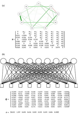
To see what such an equivalent common factor model could look like, we take as an example some network model with four nodes, in which some edge weights are constrained to zero. The model in Figure 1A represents a network model with four different edges (ω₃₁ and ω₄₁ are constrained to zero). This model thus has eight freely estimated parameters: four thresholds and four edge weights. The model in Figure 1B represents the equivalent common factor model, that results from the eigenvalue decomposition of $\mathbf{\Omega }$ in which the diagonal is set equal to −1 times the lowest eigenvalue of $\mathbf{\Omega }$ so that the lowest eigenvalue equals zero. Let Q represent the p × p eigenvector matrix in which each row is associated with an observed variable X_i and each column is associated with a latent variable η_k. Let r represent the vector of eigenvalues of the p × p covariance matrix, of which the last element equals zero such that the total number of latent variables equals p – 1. a_ik, the discrimination parameter for variable X_i on the latent variable η_k, is a function of q_ik, the eigenvector value of that variable that is associated with η_k and the eigenvalue r_k associated with η_k: $a_{ik}=-2\sqrt{r_k/2}\times q_{ik}.$ For a more extensive explanation of how to obtain A, the matrix of discrimination parameters, from $\mathbf{\Omega },$ we refer the reader to Epskamp, Maris, et al. (2018) and Marsman et al. (2015). Note that although the common factor model seems to be more complex in the number of parameters, the number of freely estimated parameters of the two models is exactly equal due to proportionality constraints on the discrimination parameters. That is, all discrimination parameters are a function of the smaller number of ω parameters.

Figure 1. The model in (1 A) represents the network model that is associated with the weight matrix $\mathbf{\Omega }.$ The model in (1B) represents the common factor model that is equivalent to the network model in (1 A). The discrimination parameters of this common factor model are presented in the matrix $\mathbf{A}.$

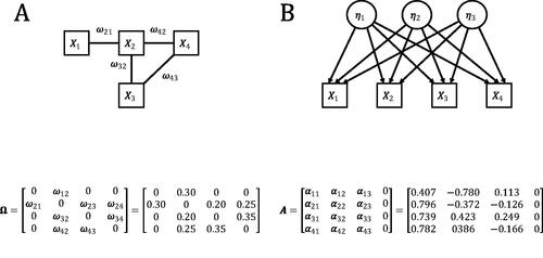
It is not clear in what cases one would consider the common factor model in Figure 1B as a plausible alternative data-generating mechanism. From a substantive point of view it is more sensible to compare the network model in Figure 1A to a common factor model with interpretable constraints, e.g. a rank constraint on the common factor model so that the number of common factors is limited. That is, in many cases the relevant comparison between two plausible explanations of the data is not a comparison between a model in the one framework and its equivalent representation in the other framework. Rather, a relevant comparison is between some specific model in the one framework that is interpretable within its framework (e.g. a common factor model with some rank constraint), and some specific model in the other framework that is also interpretable in its own framework (e.g. a network model in which some edges are constrained to zero). These models are unlikely to be equivalent, and hence can be compared empirically. In fact, in the next section we show that the group of common factor models with a single common factor and the group of network models in which some edge weights are zero, are mutually exclusive (i.e. none of the models in the one group are equivalent to any of the models in the other group). We use three diverging empirical implications of these models to make a start in statistically comparing network models and common factor models.

Distinguishing between specific models

The previous section has established that model equivalences, while important, should not be interpreted to mean that network models and latent variable models are the same. In this section, we identify divergent statistical predictions that can be derived from two important submodels that have often been proposed as candidate models in the psychological literature. First, the unidimensional factor model (UFM; Jöreskog, 1971); second, the sparse network model (SNM; Epskamp, Rhemtulla, et al., 2017). Because distributional representations become rather unwieldy for categorical variables, in this section we consider Gaussian variables.

There are two reasons for considering the group of UFMs. First, the UFM is relevant because many of the historically important psychometric models are unidimensional – examples include the models of Rasch (1960), Birnbaum (1968), Mokken (1971), and Jöreskog (1971). In fact, in several approaches the unidimensional model is used normatively in test construction; that is, violations of unidimensionality are sometimes considered a flaw of the test and can justify the removal of items (Bond & Fox, 2001). A second reason for considering UFMs is that the sets of UFMs and SNMs are mutually exclusive; there are no SNMs that are equivalent to a UFM or vice versa. Importantly, however, it is plausible to conjecture that the implications of the UFM that we use to distinguish them from SNMs also hold for other specific types of common factor models, such as correlated factor models and hierarchical factor models (van Bork, Grasman, & Waldorp, 2018); however, a proof of this conjecture falls beyond the scope of this article. If other groups of common factor models can be identified, for which these same implications hold, then these models can be distinguished from SNMs in a similar way as we show here for UFMs. Thus, establishing the procedure for the UFM provides an important starting point from which future generalizations to other models can be derived. Before we examine divergent implications that follow from these models, we briefly introduce them to the reader.

Unidimensional factor models and sparse network models

For factor models, just like for MIRT models, the observed variables are considered fallible indicators of a latent variable, which typically represents the construct of interest. Let $\Sigma$ denote the covariance matrix of y, in which y denotes a vector of p Gaussian observed variables that are mean-centered. Let η denote a Gaussian latent variable with unit variance. Let $\mathit{\lambda }$ denote the vector of factor loadings and $\Theta$ the residual covariance matrix. In a UFM all observed variables in y are a linear function of a single latent variable (η), and independent Gaussian residuals, ε: (1) $$y_i={\lambda }_i\eta +{\epsilon }_i.$$(1)

Note that because we assume normality, the UFM is a linear factor model. We let η have unit variance. The UFM implies that the covariance matrix of the indicators admits the following representation: (2) $$\Sigma =\mathit{\lambda \lambda }\prime +\Theta .$$(2)

Here, we assume that $\Theta$ is diagonal, that is, that the observed variables do not covary over and above what is explained by the latent factor. In other words, the principle of local independence holds (Bollen, 1989). Equation (2)(2) $$\Sigma =\mathit{\lambda \lambda }\prime +\Theta .$$(2) implies that the covariance among observed variables is a function of their factor loadings. 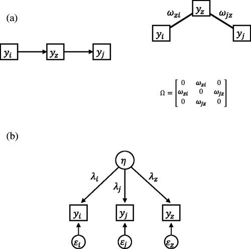More precisely, because $\Theta$ is a diagonal matrix, the covariance between two variables y_i and y_j equals ${\lambda }_i{\lambda }_j,$ in which λ_i and λ_j are elements of the vector $\mathit{\lambda }$ and denote the factor loadings of y_i and y_j on the factor η. Figure 2b depicts a factor model with three indicators.

Figure 2. (a) Direct relations underlying the correlations between $y_i,y_j\mathrm{\hspace{0.17em}\hspace{0.17em}a}\mathrm{n}\mathrm{d\hspace{0.17em}\hspace{0.17em}}{y}_z.$ The causal structure on the left implies the conditional independence structure on the right. (b) Single common cause underlying the correlations between $y_i,y_j$ and $y_z.$ Two different models that explain the correlational structure of three observed variables.

For Gaussian variables, as we consider here, the Ising network model discussed above translates into a partial correlation network. In a partial correlation network for Gaussian variables, edges have a particularly simple representation, namely as the partial correlation between two variables that results when all other variables in the network are partialled out. These partial correlations are computed by standardizing elements of the precision matrix, $\mathbf{P}={\Sigma }^{-1}:$ (3) $${\rho }_{ij·V\setminus \{i,j\}}=-\frac{p_{ij}}{\sqrt{p_{ii}{p}_{jj}}},$$(3) where $V=\{1,2,\dots ,p\}$ denotes an index set for the variables in y and $V\setminus \{i,j\}$ denotes this set minus i and j. This equation implies that off-diagonal elements of P that equal zero correspond to partial correlations of zero.

Whereas in the factor modeling approach the covariance matrix of y is a function of factor loadings and the residual covariance matrix, in the network approach the covariance matrix is defined by the following equation: (4) $$\Sigma =\Delta {(\mathbf{I}-\Omega )}^{-1}\Delta ,$$(4) where $\Omega$ is a weight matrix with zeros on the diagonal and off-diagonal elements ω_ij that reflect the edge weights between nodes, and $\Delta$ is a diagonal matrix in which the elements are functions of the diagonal elements of the precision matrix, ${\delta }_{jj}=p_{jj}^{-\frac{1}{2}}$ (Epskamp, Rhemtulla, et al., 2017).

When $\Omega$ is obtained by standardizing the inverse sample covariance matrix and multiplying the off-diagonal elements by −1, one obtains a saturated model, which perfectly reproduces the sample partial correlation matrix (Epskamp, Rhemtulla, et al., 2017). In this case, all nodes will be connected to all other nodes (with the rare exception of sample partial correlations that equal exactly zero). In practice, modelers gain degrees of freedom by assuming that the true network is sparse, that is, that relatively few direct interactions are necessary to fully explain the covariance between observed variables (Costantini et al., 2015; Deserno, Borsboom, Begeer, & Geurts, 2017; Epskamp, Rhemtulla, et al., 2017; Epskamp, Waldorp, Mõttus, & Borsboom, 2018; Isvoranu et al., 2017). Sparsity is modeled by constraining some elements of $\Omega$ to equal zero; these zeroes correspond to pairs of variables that are conditionally independent given all other variables in the network. In the following we refer to this model as a sparse network model (SNM). As such, the SNM, just like the Ising model, is a pairwise Markov Random Field (MRF; Koller & Friedman, 2009). More specifically, the SNM is a multivariate normal pairwise MRF, which is known as a Gaussian Graphical Model (GGM; Lauritzen, 1996). A pairwise MRF is an undirected network in which nodes represent observed random variables and any edge between two nodes represents the conditional dependence between these nodes given all other nodes in the network. Correspondingly, any missing edge represents a conditional independence between these nodes given all other nodes and as such a MRF encodes the conditional independence structure of a set of nodes.

Divergent implications

When considering two specific models, such as the UFM and SNM, rather than two general model classes (e.g. all factor models versus all network models), we can derive targeted comparisons of particular phenomena in the data for which the relevant models have divergent statistical predictions. We explicate one such implication in this section.

Partial correlations and zero-order correlations

For unidimensional factor models, each partial correlation lies between zero and the zero-order correlation (van Bork et al., 2018). This implication does not rely on properties of the normal distribution and thus extends to other unidimensional factor models than the linear factor model. This result includes three more specific implications of UFMs: (1) the UFM implies that partial correlations cannot equal zero, (2) the UFM implies that partial correlations cannot switch sign compared to the zero-order correlation and (3) the UFM implies that partial correlations cannot be greater in absolute value than the zero-order correlation. In the following we will explain these three implications. We consider standardized variables so that $\Sigma$ simplifies to a correlation matrix. The factor loadings are interpretable as standardized regression coefficients. We assume that the diagonal matrix $\Theta$ is positive definite, so that factor loadings are never exactly −1 or 1. We also assume that factor loadings are never 0. Note that the implications that we demonstrate extend to unstandardized variables because they rely on Equation (2)(2) $$\Sigma =\mathit{\lambda \lambda }\prime +\Theta .$$(2) , which also holds for an unstandardized $\Sigma$ and $\mathit{\lambda }$ and the status of the parameters in $\Theta$ is irrelevant.

Partial correlations of zero

Let y_i, y_j and y_z be elements of y, the vector of observed variables. The partial correlation between y_i and y_j given y_z is defined as follows (Chen & Pearl, 2014): (5) $${\rho }_{ij.z}=\frac{{\rho }_{ij}-{\rho }_{iz}{\rho }_{jz}}{\sqrt{(1-{\rho }_{iz}^2)(1-{\rho }_{jz}^2)}}$$(5)

Figure 2 shows two possible causal mechanisms that result in nonzero correlations between y_i, y_j and y_z. In Figure 2a, two direct relations (ω_zi and ω_jz) cause all three variables to be correlated. By plugging in the correlations that correspond to Figure 2a (${\rho }_{iz}={\omega }_{zi},{\rho }_{jz}={\omega }_{jz}$ and ${\rho }_{ij}={\omega }_{zi}{\omega }_{jz}$) in Equation (5)(5) $${\rho }_{ij.z}=\frac{{\rho }_{ij}-{\rho }_{iz}{\rho }_{jz}}{\sqrt{(1-{\rho }_{iz}^2)(1-{\rho }_{jz}^2)}}$$(5) , the numerator of Equation (5)(5) $${\rho }_{ij.z}=\frac{{\rho }_{ij}-{\rho }_{iz}{\rho }_{jz}}{\sqrt{(1-{\rho }_{iz}^2)(1-{\rho }_{jz}^2)}}$$(5) becomes zero. If a common factor underlies the covariance of y_i, y_j, and y_z (depicted in Figure 2b), however, ${\rho }_{ij.z}$ cannot equal zero. It follows from Equation (2)(2) $$\Sigma =\mathit{\lambda \lambda }\prime +\Theta .$$(2) that, if y_i, y_j and y_z are influenced by a single common factor like in Figure 2b, their correlations can be expressed as follows: (6) $$\begin{array}{c}{\rho }_{ij}={\lambda }_i{\lambda }_j\\ {\rho }_{iz}={\lambda }_i{\lambda }_z\\ {\rho }_{jz}={\lambda }_j{\lambda }_z\end{array}$$(6)

The partial correlation ${\rho }_{ij.z}$ equals zero when ${\rho }_{ij}={\rho }_{iz}{\rho }_{jz}.$ Using expression 6, in the case of a UFM, this equivalence holds if and only if ${\lambda }_i{\lambda }_j=({\lambda }_i{\lambda }_z)({\lambda }_j{\lambda }_z),$ which only holds if either λ_i or λ_j equals zero, or when ${\lambda }_z=1$ or ${\lambda }_z=-1.$ Put differently, partial correlations of zero in a UFM coincide with standardized factor loadings of zero, one or minus one. A standardized factor loading of zero implies that the corresponding variable does not load on the common factor and thus none of its correlations with other variables can be explained by the common factor. A variable with a standardized factor loading of 1 or −1 is perfectly correlated with the latent factor, which, as a result, is no longer latent. In this case, the common factor is observed, and conditioning on the variable with factor loading 1 or −1 would render all other variables statistically independent, due to the assumption of local independence (Bollen, 1989).

Holland and Rosenbaum (1986) proved that the simple example above with three observed variables applies to all UFMs; that is, UFMs imply that partial correlations between the observed variables can never be exactly zero. However, do note that, given a unidimensional factor model, as the set of observed variables increases (i.e. as y contains more elements), partial correlations may become very small, as the set of observed variables partialled out yields an increasingly better approximation to the latent factor (see also, Guttman, 1940, 1953). This suggests that, unless one has access to a very large sample so that one can distinguish between zero partial correlations and very small partial correlations, this divergent implication may be most efficiently utilized for relatively small sets of variables.

Sign switch in partial correlations

Holland and Rosenbaum (1986) also showed that UFMs imply that the partial correlation has to have the same sign as the zero-order correlation. Consider the earlier example with three variables y_i, y_j and y_z again. The denominator in Equation (5)(5) $${\rho }_{ij.z}=\frac{{\rho }_{ij}-{\rho }_{iz}{\rho }_{jz}}{\sqrt{(1-{\rho }_{iz}^2)(1-{\rho }_{jz}^2)}}$$(5) is positive. This means that if ρ_ij is positive, the partial correlation ${\rho }_{ij.z}$ only switches sign (i.e. is negative) when the numerator ${\rho }_{ij}-{\rho }_{iz}{\rho }_{jz}$ is negative. Suppose now that y_i, y_j and y_z are indicators in a UFM. If ρ_ij is positive, then ${\lambda }_i{\lambda }_j$ is positive. This means that the numerator in Equation (5)(5) $${\rho }_{ij.z}=\frac{{\rho }_{ij}-{\rho }_{iz}{\rho }_{jz}}{\sqrt{(1-{\rho }_{iz}^2)(1-{\rho }_{jz}^2)}}$$(5) cannot be negative since we established that for a UFM the numerator equals ${\lambda }_i{\lambda }_j-({\lambda }_i{\lambda }_z)({\lambda }_j{\lambda }_z)$ which equals ${\lambda }_i{\lambda }_j-{\lambda }_i{\lambda }_j{\lambda }_z^2.$ For this to be negative ${\lambda }_z^2$ has to be larger than one. In contrast, a network model does not imply that the partial correlation should have the same sign as the zero-order correlation. Collider structures in which two variables have a common effect, are a well known example in which the correlation between the causes can be (slightly) positive but the partial correlation between the causes conditioning on the common effect is negative (Lauritzen, 1996; Pearl, 2000). For example, when y_i and y_j have a weak positive correlation but both have a strong positive influence on y_z, then the partial correlation between y_i and y_j given y_z will be negative. This result suggests that the observation of partial correlations that have a different sign than the zero-order correlation indicate evidence in favor of an SNM over a UFM.

Increase in absolute partial correlations

The third implication of a UFM that diverges from an SNM, is that partial correlations between two indicators in a UFM cannot be stronger than the corresponding zero-order correlation between these indicators. That is, the absolute partial correlation between two variables can never be larger than the corresponding absolute zero-order correlation.

To get an intuitive sense for why this implication follows, consider again Equation (5)(5) $${\rho }_{ij.z}=\frac{{\rho }_{ij}-{\rho }_{iz}{\rho }_{jz}}{\sqrt{(1-{\rho }_{iz}^2)(1-{\rho }_{jz}^2)}}$$(5) . Suppose that ρ_ij is positive, then ${\rho }_{ij.z}$ is stronger than ρ_ij only if ${\rho }_{iz}{\rho }_{jz}$ is negative. For ${\rho }_{iz}{\rho }_{jz}$ to be negative, either ρ_iz or ρ_jz has to be negative, but not both. That is, exactly one of the three correlations must be negative. Suppose that ρ_ij is negative, then ${\rho }_{ij.z}$ is stronger than ρ_ij only if ${\rho }_{iz}{\rho }_{jz}$ is positive. For ${\rho }_{iz}{\rho }_{jz}$ to be positive both ρ_iz and ρ_jz have to be negative or both ρ_iz and ρ_jz have to be positive. As a result, for any three variables there are two correlational structures that result in partial correlations that are stronger than the corresponding zero-order correlations: (I) one negative correlation and two positive correlations or (II) three negative correlations.

Neither of these two correlational structures, however, can be explained by a UFM, as becomes clear from examining expression (6). Given any three variables, to arrive at a correlational structure with either one or three negative correlations at least one factor loading ought to be negative. However, both one and two negative factor loadings result in two negative correlations, while three negative factor loadings results in no negative correlations. In sum, there is no way to choose factor loadings such that the model results in a correlation structure that complies with partial correlations that are stronger than their corresponding zero-order correlations.

The above example extends to more than three variables. Let ${\widehat{y}}_{i;V\setminus \{i,j\}}$ and ${\widehat{y}}_{j;V\setminus \{i,j\}}$ denote the best linear approximation of respectively y_i and y_j in terms of the variables that are partialled out, $V\setminus \{i,j\}$ (i.e. the variation in y_i that is explained by $V\setminus \{i,j\}$). The residual of y_i is $y_i-{\widehat{y}}_{i;V\setminus \{i,j\}}$ and is denoted as ${\widehat{y}}_{i·V\setminus \{i,j\}}$ (because it represents the part of y_i that is not predicted by other variables in y). The partial correlation between y_i and y_j (denoted ${\widehat{\rho }}_{ij·V\setminus \{i,j\}}$) is the zero-order correlation between ${\widehat{y}}_{i·V\setminus \{i,j\}}$ and ${\widehat{y}}_{j·V\setminus \{i,j\}}$ (i.e. between the residuals² of y_i and y_j; Cramér, 1946).

In any UFM, each observed variable (y_i) is a function of the factor (η) and some random error (${\epsilon }_i$). The principle of local independence implies that the observed variables only share variance due to η. Thus, by subtracting a linear combination of the other observed variables from both y_i and y_j, variance related to η is pulled out, while none of the random error (${\epsilon }_i$ or ${\epsilon }_j$) is pulled out as this is not shared with the other observed variables. Because η is precisely what y_i and y_j share, the correlation between ${\widehat{y}}_{i·V\setminus \{i,j\}}$ and ${\widehat{y}}_{j·V\setminus \{i,j\}}$ (i.e. the partial correlation between y_i and y_j) must be smaller in absolute size than the zero-order correlation. Note that the partial correlation does not become zero because the observed variables that are partialled out also contain random error. However, if any of the partialled-out variables contained no measurement error, all of η would be subtracted from y_i and y_j, resulting in a partial correlation of zero. This is in correspondence with the previous section, in which we showed that partial correlations can only equal zero if at least one standardized factor loading equals one (i.e. there is no measurement error). For a complete proof of the general case with p variables see (van Bork et al., 2018).

The partial correlation likelihood test

In the previous section, we discussed three diverging predictions for empirical data: (1) UFMs imply that the population partial correlations cannot equal zero (2) UFMs imply that population partial correlations cannot have a different sign than the corresponding zero-order correlations and (3) UFMs imply that the population partial correlations cannot be stronger than the corresponding zero-order correlations. None of these three implications hold for SNMs. Considering these alternative hypotheses of SNMs versus UFMs, we can assess whether the proportion of partial correlations that have a different sign than the corresponding zero-order correlations in the data is more consistent with a UFM or with an SNM. We can also assess whether the proportion of partial correlations that are stronger than the corresponding zero-order correlations in the data is more consistent with a UFM or with an SNM. We cannot assess the number of partial correlations in the data that are exactly zero, since sample partial correlations will rarely be exactly zero even when the population partial correlation is zero. We could circumvent this problem by assessing the proportion of partial correlations that are significantly different from zero, but since the UFM implies very small partial correlations (especially with more indicators or stronger factor loadings) it is difficult to determine when the power is sufficient to detect partial correlations that are zero. We therefore use (2) and (3) to construct a likelihood test that compares UFMs with SNMs.

The proportion of partial correlations that are inconsistent with a UFM (either because they have a different sign than the zero-order correlation, or because they are greater in absolute value than the zero-order correlation) can be interpreted as a test statistic, and the value of this test statistic can be compared to the sampling distribution that would arise (a) under the hypothesis that the best-fitting UFM were true, and (b) under the hypothesis that the best-fitting SNM were true. The relevant sampling distributions, while analytically intractable, are not difficult to simulate. Appendix A provides code to get sampling distributions for the proportion of partial correlations that either have a different sign than the zero-order correlation or are greater in absolute value than the zero-order correlation, under the best-fitting UFM and SNM. The resulting test, which we will refer to as the Partial Correlation Likelihood (PCL) test, works as follows:

1. The sample covariance matrix is used to obtain a sample partial correlation matrix. The proportion of partial correlations that either have the opposite sign as the zero-order correlation or are greater in absolute value than the zero-order correlation, is calculated.

2. Both a UFM and an SNM are estimated from the sample covariance matrix using maximum likelihood estimation, resulting in ML(UFM) and ML(SNM).

3. The model implied covariance matrices of both models are obtained: ${\widehat{\Sigma }}_{\mathit{UFM}}$ and ${\widehat{\Sigma }}_{\mathit{SNM}}.$

4. ${\widehat{\Sigma }}_{\mathit{UFM}}$ and ${\widehat{\Sigma }}_{\mathit{SNM}}$ are each used to simulate 1000 datasets of size N.

5. For each dataset the proportion of partial correlations that either have the opposite sign as the zero-order correlation or are greater in absolute value than the zero-order correlation, is calculated. These proportions are used to create a probability mass function for each model.

6. The observed proportion in the sample is compared to the probability mass functions of ML(UFM) and ML(SNM). The results are combined in a decision procedure. For example, one can decide that the model that assigns the highest probability mass to the observed proportion ‘wins’ the test. Alternatively, one could calculate a likelihood ratio and make a decision when the likelihood ratio is larger than some specified value.

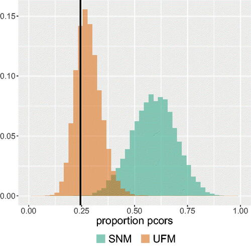
Figure 3 represents how the test works and Figure 4 shows an example of test results on data that were simulated under a UFM with 10 variables. The graph presents information about how much more probable the observed proportion is under the one model than under the other model.

Figure 3. A visual representation of how the test works. The numbers 1:6 correspond with the steps explained in the text. The sample covariance matrix results in two estimated models that both correspond to a probability mass function. The model with the highest probability mass for the observed proportion wins the test. See text for detail.

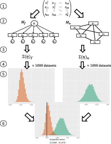
Figure 4. An example of possible output of the test. The black vertical line represents the observed proportion of partial correlations that switched sign or increased in absolute value. In this example the observed proportion in the data has a higher probability mass under the UFM than under the SNM.

The likelihood of the SNM is the probability of the observed proportion of partial correlations that switched signs under the best-fitting SNM (i.e. $P(x|\text{ML}(\text{SNM})),$ in which x denotes the observed proportion in the data). Similarly, $P(x|\text{ML}(\text{UFM}))$ is the likelihood of the UFM. These likelihoods can be used to calculate a ratio of likelihoods which yields a similar interpretation to other evidence ratios that are based on a ratio of likelihoods in combination with a function of the number of free parameters to account for model complexity. For example, the ratio of Akaike weights can be rewritten as $\frac{L_i}{L_j}\hspace{0.17em}\text{exp}\hspace{0.17em}(F_j-F_i)$ where L_i is the maximum likelihood for model M_i, and F_i the number of free parameters (Wagenmakers & Farrell, 2004). For the best-fitting SNM and best-fitting UFM, the number of free parameters is zero ($F_{\mathit{UFM}}=F_{\mathit{SNM}}=0$) and thus the ratio of Akaike weights equals the ratio of likelihoods. Other evidence ratios that compare the likelihoods of two models while accounting also for model complexity are the Bayes factor and the ratio of BIC weights. The ratio of BIC weights equals $\frac{L_i}{L_j}{n}^{\frac{1}{2}(F_j-F_i)}$ in which n is the number of observations (Wagenmakers & Farrell, 2004). With equal numbers of free parameters the ratio of BIC weights reduces to $\frac{L_i}{L_j}:$ the ratio of likelihoods. Similarly, the Bayes factor reduces to a likelihood ratio when the models that are compared have no free parameters (Kass & Raftery, 1995). For more information on likelihoods as measures of statistical evidence in the likelihoodist framework we refer the reader to Edwards (1972) and Royall (1997).

Simulation study

We conducted a Monte Carlo study in R (R Core Team, 2018) to examine the performance of the PCL test when the true model that underlies the data (SNM or UFM) is known. Test performance is evaluated using the proportion of replications in which the test chooses the true underlying model.

Simulation design

We generated sample covariance matrices for a set of 10 variables according to either a UFM or an SNM with edge density .5 (i.e. 50% of the possible edges were set to zero). To explore the influence of power on test performance, we generated data with sample sizes ranging from 100 to 2000, in steps of 100. For each combination of model and sample size, we generated 1000 sample covariance matrices on which the test was performed. As the number of variables in the model influences the strength of partial correlations in a UFM, we repeated this simulation for 5 and 15 variables. To consider a possible influence of the network density (i.e. the proportion of non-zero edges in a network), we also repeated the simulation for edge densities of .2 and .8 (with 10 variables only). Finally, we repeated the simulation for all conditions with cross-validation. In these simulations, one half of the data is used to estimate the UFM, SNM, and probability mass functions from these models. The other half of the data is used to obtain the observed proportion of partial correlations that either switched in sign or are greater in absolute value than the zero-order correlation. The observed proportion obtained in step two is then compared to the probability mass functions that are obtained in step one.

Generating data from SNMs and UFMs

An SNM was generated by constructing a precision matrix, $\mathbf{P}={\Sigma }^{-1},$ for which each element is specified to be either zero or sampled from a uniform distribution over the interval [−1, 1]. First, the diagonal was set to zero, and then the eigenvalues were computed. To make the matrix positive definite, the diagonal was set to the smallest eigenvalue plus an arbitrary small number (0.2). After this, the matrix was forced to be symmetric using the forceSymmetric() function of the R-package ‘Matrix’ (Bates & Maechler, 2014). The resulting precision matrix P is related to the network weight matrix $\Omega$ (i.e. the partial correlation matrix) as follows: (7) $$\begin{array}{c}\mathbf{P}={\Delta }^{-1}(\mathbf{I}-\Omega ){\Delta }^{-1}\\ \Omega =\mathbf{I}-\Delta \mathbf{P}\Delta \end{array}$$(7) where $\Delta$ is a diagonal matrix with ${\delta }_{jj}=p_{jj}^{-\frac{1}{2}}.$ To obtain the weight matrix $\Omega ,$ P is pre- and post-multiplied by $\Delta ,$ yielding a standardized precision matrix, which is subtracted from an identity matrix, to change the sign of all off-diagonal elements. Note that all elements that equal zero in the precision matrix will also equal zero in the weight matrix, that is, they correspond to missing edges in the network. The correlation matrix that corresponds to the obtained weight matrix was used to simulate data.

To construct covariance matrices consistent with a factor model, we sampled factor loadings from a uniform distribution over the interval [0.1, 0.9] and [−0.9,−0.1] to exclude factor loadings equal to zero, one or minus one. These factor loadings were combined in a vector $\mathit{\lambda }$ which we used to obtain a correlation matrix in the following way: (8) $$\Sigma =\mathit{\lambda \lambda }\prime +\Theta ,$$(8) in which $\Theta$ is a diagonal matrix with ${\theta }_{ii}=1-{\lambda }_i^2.$

We used the function mvrnorm() of the R-package ‘MASS’ (Venables & Ripley, 2002) to simulate data from the constructed covariance matrices.

Estimating models from generated data

The test was performed in R (R Core Team, 2018). The R-package ‘lavaan’ (Rosseel, 2012) was used to estimate a UFM from the sample covariance matrix and to retrieve a model implied covariance matrix for this estimated factor model. A network model was estimated from the sample covariance matrix with the function EBICglasso() from the R-package ‘qgraph’ (Epskamp, Cramer, Waldorp, Schmittmann, & Borsboom, 2012). This function estimates $\widehat{\mathbf{P}},$ the precision matrix, by introducing a lasso penalty on the sum of the elements in the lower triangle of $\widehat{\mathbf{P}}$ such that many of the elements in $\widehat{\mathbf{P}}$ are set to exactly zero (Friedman, Hastie, & Tibshirani, 2008). A regularization parameter determines the weight of the penalty in obtaining $\widehat{\mathbf{P}},$ such that higher values of the regularization parameter result in more elements in $\widehat{\mathbf{P}}$ being put to zero than lower values of the regularization parameter. This penalization parameter is determined by minimizing the Extended Bayesian Information Criterion (EBIC; Foygel & Drton, 2010). Note that because $\widehat{\mathbf{P}}$ will have elements that are exactly zero, $\Omega$ will have this as well (see Equation 7(7) $$\begin{array}{c}\mathbf{P}={\Delta }^{-1}(\mathbf{I}-\Omega ){\Delta }^{-1}\\ \Omega =\mathbf{I}-\Delta \mathbf{P}\Delta \end{array}$$(7) ), and thus the estimated network will be a sparse network. Note that the estimation procedures described in this paragraph refer to step (2) of the test, and that the likelihoods that are used in this step to obtain the best-fitting UFM and SPM are not the likelihoods on which the SPM and UFM are being compared in step (5) of the test.

Results simulation study

Table 1 presents the results of the simulation study for the PCL test for 5, 10 and 15 observed variables. The most important results are also included in the graph in Figure 5. The numbers in Table 1 represent the correct (c) and incorrect (i) decision rates in percentages of cases for both cases in which the true model is a UFM and cases in which the true model is an SNM, as well as for different numbers of variables and densities. The green line with crosses in Figure 5 corresponds to the correct decision rate. The blue (circles), orange (solid), and yellow (dashed) lines present the mean proportions of partial correlations that have the opposite sign as the zero-order correlation or are stronger than the zero-order correlation, that are present in the sample data and implied by the two estimated models (yellow (dashed) = implied by the SNM, orange (solid) = implied by the UFM). In cases where an SNM is the true model, the yellow (dashed) line should trace the blue (circles) line closer, and in cases where a UFM is the true model, the orange (solid) line should trace the blue (circles) line closer.

Figure 5. Performance of the test for 5, 10, and 15 variables with the number of observations on the horizontal axis. The green line with crosses represents the proportion of replications in which the test picked the correct model (for 5a, 5c and 5e this is an SNM and for 5 b, 5d and 5f this is a UFM). The blue line represents the mean proportion of partial correlations that have a different sign than the zero-order correlation or are greater in absolute value than the zero-order correlation in data sets that are generated from the true model. The dashed yellow line represents this mean proportion for the estimated SNM and the solid orange line represents this mean proportion for the estimated UFM.

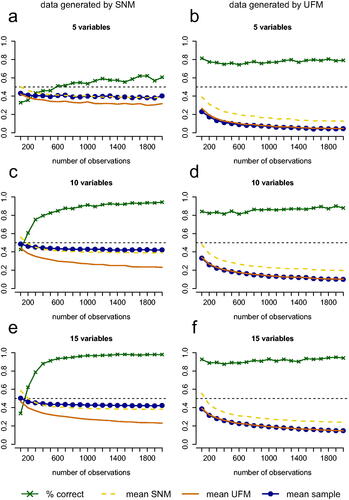
Table 1. Percentage of cases in which the PCL test made a correct (c) or incorrect (i) decision on whether a UFM or SNM underlies the data. The results in this table stem from simulations in which the test picked the model with the highest likelihood for the observed proportion significant partial correlations in the data. The percentages correct and incorrect decisions do not always add up to 100. The missing percentage is the percentage of cases in which the test did not decide because the SNM and UFM had the same likelihood.

N
Density	# Variables	Decision	100	200	300	400	500	600	700	800	900	1000	1100	1200	1300	1400	1500	1600	1700	1800	1900	2000
–	5	c	81.4	77.4	76.6	74.8	76.1	74.3	76.1	77.7	75.7	77.0	77.0	78.8	79.7	77.0	79.0	79.7	78.9	80.5	78.6	79.1
–	5	i	18.3	22.4	23.3	25.2	23.7	25.6	23.7	21.8	23.7	22.3	22.6	20.6	19.7	21.6	19.9	18.8	19.3	18.1	17.8	18.3
–	10	c	84.1	82.2	83.3	81.4	84.4	81.3	83.2	86.3	85.8	86.3	85.8	86.4	86.9	87.0	86.5	87.9	89.4	87.2	90.0	87.9
–	10	i	15.8	17.7	16.7	18.4	15.2	18.6	16.6	13.5	14.2	13.7	13.9	13.5	12.9	12.9	13.5	12.0	10.5	12.7	9.7	12.0
–	15	c	92.7	88.7	89.3	87.4	89.1	88.6	89.7	91.5	90.7	93.0	90.8	92.7	91.1	90.3	93.6	92.8	93.3	94.4	95.0	94.2
–	15	i	7.0	11.2	10.5	12.4	10.5	10.9	10.1	8.4	9.0	6.9	9.1	7.2	8.5	9.7	6.3	7.0	6.4	5.6	5.0	5.8
0.5	5	c	32.9	35.6	43.4	45.8	46.0	51.2	51.6	54.3	54.8	53.6	56.8	59.1	57.5	57.3	55.4	58.6	62.0	62.1	56.8	60.6
0.5	5	i	66.2	63.6	56.0	53.3	53.4	48.2	47.8	44.7	44.2	45.8	42.7	40.5	42.4	42.2	44.2	40.6	37.4	37.0	42.8	38.9
0.5	10	c	42.6	60.7	75.3	79.5	82.5	84.8	87.7	87.3	89.6	91.2	89.5	91.5	92.6	91.9	92.1	93.4	92.8	93.6	93.5	94.3
0.5	10	i	57.0	38.2	24.6	19.8	17.4	14.9	11.7	12.5	9.8	8.5	10.3	8.2	7.2	8.0	7.8	6.5	6.6	6.2	6.2	5.6
0.5	15	c	33.7	62.2	78.7	87.9	91.2	93.5	94.2	95.0	96.0	96.8	96.6	97.1	97.3	98.0	98.1	97.8	97.3	97.9	98.0	97.9
0.5	15	i	65.7	37.1	20.4	11.4	8.3	6.0	4.5	4.1	3.0	2.7	2.8	2.2	1.8	1.4	1.1	1.3	1.6	1.3	1.1	1.4
0.2	10	c	40.0	46.1	51.9	55.3	52.7	56.0	57.4	55.3	58.8	57.2	60.0	62.2	59.5	60.5	61.7	63.6	61.6	61.2	65.1	61.6
0.2	10	i	59.0	52.4	46.7	43.3	46.6	42.7	41.4	43.6	39.8	42.0	38.6	36.4	39.5	38.4	37.7	35.4	37.6	37.4	34.3	37.4
0.8	10	c	51.1	75.4	86.1	90.2	92.7	93.7	95.2	95.9	95.8	95.7	96.2	95.5	97.6	95.9	97.3	97.7	97.6	97.2	97.1	97.6
0.8	10	i	48.4	24.5	13.4	9.1	7.1	5.8	4.7	3.8	3.6	3.9	3.7	4.0	2.0	3.5	2.4	1.7	2.2	2.4	2.4	2.4

Number of observations

The performance of the test generally improves as the number of observations increases. When the true model is an SNM, the improvement in performance for increasing numbers of observations is particularly strong for small numbers of observations. For example, with 10 observed variables, the test correctly picks the SNM as the more likely model in only 43% of the cases with 200 observations (see Table 1 and Figure 5c) while this is already 83% with 500 observations and 94% with 2000 observations. When the true model is a UFM, the performance improves only very slightly with increasing numbers of observations. For example, with 10 observed variables, the test correctly picks the UFM as the more likely model in 80% to 90% of the cases for all numbers of observations that are considered (see Table 1 and Figure 5d).

Number of variables

As the number of variables increases, the performance of the test improves both when an SNM underlies the data and when a UFM underlies the data. The number of variables has a stronger impact on the performance of the test when an SNM underlies the data then when a UFM underlies the data. For example, with 5 variables, when an SNM underlies the data, the test only picks the right model in 61% of the cases with 2000 observations. It is therefore not recommended to use this test for such small numbers of variables.

Network density

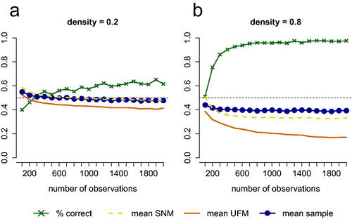
In the results presented so far, data were simulated from SNMs with a density of 0.5 (i.e. the probability of an edge in the network being present was 0.5). Figure 6 presents simulation results for 10 variables when the data-generating model is an SNM with density 0.2 (Figure 6a) or an SNM with density 0.8 (Figure 6b). The results indicate that when the true model is an SNM, a higher density results in a better test performance.

Figure 6. Performance of the test for 10 variables when (a) an SNM with density 0.2 or (b) an SNM with density 0.8 underlies the data. The green line with crosses represents the proportion of simulated cases in which the test picks the right model (for both (a) and (b) this is an SNM). The blue line represents the mean proportion of partial correlations that have a different sign than the zero-order correlation or are greater in absolute value than the zero-order correlation in data sets that are generated from the true model. The dashed yellow line represents this mean proportion for the estimated SNM and the solid orange line represents this mean proportion for the estimated UFM.

Cross-validation results

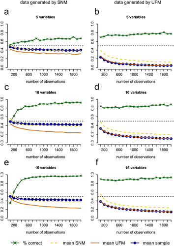
The results of the simulations with the cross-validation scheme suggest that the performance of the PCL test holds up under cross-validation (see Figure 7). In fact, for the condition with 5 variables and in which an SNM underlies the data, the results of the test were slightly better in the simulations with cross-validation than without cross-validation (see Figures 5a and 7a).

Figure 7. Performance of the test with cross-validation for conditions with 5, 10, and 15 variables with the number of observations on the horizontal axis. The green line with crosses represents the proportion of replications in which the test picked the correct model (for 5a, 5c and 5e this is an SNM and for 5 b, 5d and 5f this is a UFM). The blue line represents the mean proportion of partial correlations that have a different sign than the zero-order correlation or are greater in absolute value than the zero-order correlation in data sets that are generated from the true model. The dashed yellow line represents this mean proportion for the estimated SNM and the solid orange line represents this mean proportion for the estimated UFM.

Reasoning with equivalence and testability: a practical example

The above discussion of equivalence and testability suggests that, in practical research situations, model equivalences can sharpen and inform the way researchers approach their data. For instance, the equivalence proofs can be used to construct alternative hypotheses about the data-generating mechanism, by considering which latent variable model would be able to mimic data from a network or vice versa (see Epskamp, Kruis, & Marsman, 2017, for some examples). In addition, the divergent statistical predictions identified in this article can be used to gain insight into the relative likelihoods of particular models under investigation. To illustrate this, we examine a dataset containing items designed to assess procrastination. We consider the alternative hypotheses that the item responses arise from a UFM or from an SNM.

The dataset consists of 414 observations on items of the Irrational Procrastination Scale (IPS; Steel, 2010), and is part of an ongoing data collection program of the Allameh Tabataba’i University in Tehran. The IPS is a self-report measure of procrastination consisting of nine items that are scored on a 5-point Likert scale. The items and the polychoric correlation matrix of the data are included in Appendix B and Table 2 respectively. The internal consistency of the IPS is $\alpha =0.91$ in the validation sample (Steel, 2010), and $\alpha =0.81$ in the sample we use for our analyses. We used the polychoric correlation matrix of these 9 variables to estimate a UFM and SNM (see Table 2). Steel (2010) found that a single factor was sufficient to explain the data. These findings have been replicated in other samples which resulted in the same conclusion of a single dimension underlying the procrastination items (Rozental et al., 2014; Svartdal, 2017). Rozental et al. (2014) actually found a second factor for the reversed items but concluded that this is an artifact reflecting that participants missed the negation in these items.

Table 2. Polychoric correlation matrix of the 9 procrastination items. This correlation matrix is obtained with cor_auto() of the R-package qgraph (Epskamp et al. 2012).

	V1	V2	V3	V4	V5	V6	V7	V8	V9
V1	1.000	0.187	0.476	0.517	0.393	0.399	0.520	0.529	0.272
V2	0.187	1.000	−0.097	0.304	0.047	0.439	0.264	0.309	0.426
V3	0.476	−0.097	1.000	0.436	0.557	0.260	0.394	0.395	0.086
V4	0.517	0.304	0.436	1.000	0.476	0.351	0.576	0.520	0.320
V5	0.393	0.047	0.557	0.476	1.000	0.422	0.508	0.502	0.178
V6	0.399	0.439	0.260	0.351	0.422	1.000	0.492	0.531	0.449
V7	0.520	0.264	0.394	0.576	0.508	0.492	1.000	0.740	0.291
V8	0.529	0.309	0.395	0.520	0.502	0.531	0.740	1.000	0.368
V9	0.272	0.426	0.086	0.320	0.178	0.449	0.291	0.368	1.000

The best-fitting UFM is represented in Figure 8a. The equivalent network model is represented in Figure 8b. To get this network we let Σ in Equation (4)(4) $$\Sigma =\Delta {(\mathbf{I}-\Omega )}^{-1}\Delta ,$$(4) equal the covariance matrix that is implied by the UFM (i.e. all covariances in Σ are a function of the nine factor loadings). We then get Ω from Σ by taking the inverse of Σ and multiplying all off-diagonal elements with −1, and then standardizing the resulting matrix (i.e. using Equation (4)(4) $$\Sigma =\Delta {(\mathbf{I}-\Omega )}^{-1}\Delta ,$$(4) ). The elements in Ω correspond to partial correlations that are implied by the UFM. Note here that the number of parameters is not equal to the number of non-zero edges: the network is a complete graph but all edge weights are a function of the nine factor loadings. The best-fitting SNM is represented in Figure 9a. The covariance matrix of the estimated SNM is positive definite, so we can interpret the eigenvalue decomposition as a representation of a common factor model. The covariance matrix that is implied by the best-fitting SNM is of full rank and thus the eigenvalue decomposition results in as many factors as observed variables, i.e. all nine positive eigenvalues can be seen to represent a factor. This factor solution is represented in Figure 9b.

Figure 8. (a) The UFM that was estimated from the item responses in the procrastination dataset. The estimated factor loadings are standardized. (b) The network that is equivalent to the estimated UFM in Figure 8a. All weights are a function of the nine factor loadings, so that the weights conform to a rank one matrix. Note that the network is not an SNM; it is a complete graph.

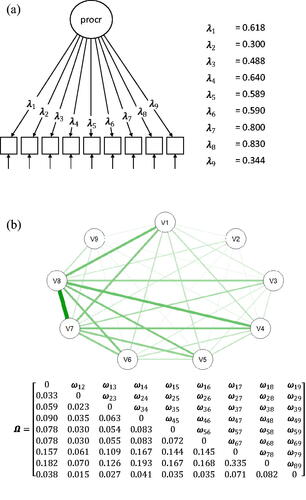
Figure 9. (a) The SNM that was estimated from the item responses in the procrastination dataset. (b) The eigenvalue decomposition of the correlation matrix implied by the SNM in Figure 9a. Q is a matrix of the eigenvectors and r is a vector of the eigenvalues. Estimated SNM and the equivalent common factor model.

The interesting comparison here is not between the UFM and its equivalent network model (the models in Figure 8a and b) or between the SNM and its equivalent latent variable model (the models in Figure 9a and b), but rather between the best-fitting SNM and best-fitting UFM, and these two classes of models (UFMs and SNMs) diverge in their predictions for empirical data, making them distinguishable.

We applied the PCL test to the data on the nine procrastination items. This analysis can be replicated with the polychoric correlation matrix of the procrastination data that is included in Table 2. Figure 10 shows the sampling distributions of the test statistic under the best-fitting UFM and the best-fitting SNM for the nine procrastination items. The vertical black line represents the observed proportion of partial correlations in the procrastination data that have a different sign than their corresponding zero-order correlation or are greater in absolute value than the zero-order correlation.

Figure 10. The probability mass functions of the best-fitting SNM and UFM for the proportion of partial correlations that either have the opposite sign as their corresponding zero-order correlations or are greater in absolute value than their corresponding zero-order correlations. The black vertical line represents the observed proportion in the data.

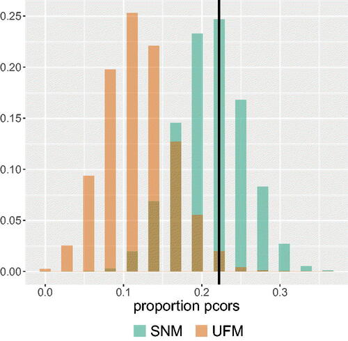
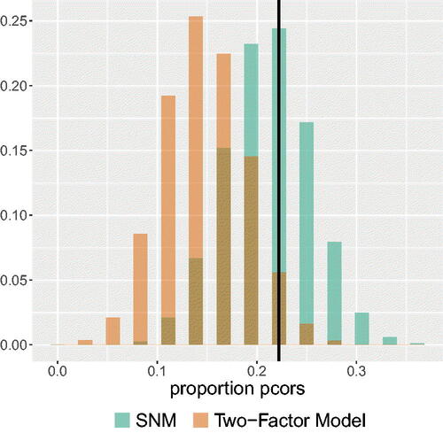
As we can see from Figure 10, the best-fitting SNM has a higher likelihood given the observed proportion of partial correlations that switched sign or are greater in absolute value than the zero-order correlation, than the best-fitting UFM. The best-fitting SNM assigns a probability of 0.246 to this observed proportion of partial correlations in the data. The best-fitting UFM assigns a probability of only 0.020 to the observed proportion in the data. So, the observed proportion of partial correlations that have the opposite sign or are greater in value than the zero-order correlation is more probable under the estimated SNM than under the estimated UFM. To investigate whether the lower likelihood of the UFM is not merely the result of a second factor that underlies the data on which the reversed items load, we repeated the analysis with the test comparing the best-fitting SNM to the best-fitting correlated two-factor model. An exploratory factor analysis on the data indicated that only the reversed items loaded higher on the second factor than on the first factor. We therefore estimated a factor model in which the items that were not reversed loaded on one factor and the reversed items loaded on a second factor. As shown in Figure 11, the results were similar, providing support for an SNM over a correlated two-factor model.

Figure 11. The probability mass functions of the best-fitting SNM and best-fitting correlated two-factor model for the proportion of partial correlations that either have the opposite sign as their corresponding zero-order correlations or are greater in absolute value than their corresponding zero-order correlations. The black vertical line represents the observed proportion in the data.

The results of this comparison suggest that a focus on the relation between the partial correlations and zero-order correlations in the data provides evidence for the estimated SNM over the estimated UFM. Given the observed proportion of partial correlations that have a different sign than the zero-order correlation or are stronger than the zero-order correlation, the SNM has a higher likelihood than the UFM.

Discussion

Psychology has a history of modeling theoretical constructs as latent factors that act as common determinants for a set of observed variables (e.g. Caspi et al., 2014; McCrae & Costa, 1987; Spearman, 1904). In the past decade, however, multiple studies have shown that networks offer reasonable alternative ways of understanding such constructs (e.g. Cramer et al., 2012; McNally et al., 2014; Van der Maas et al., 2006). At this point in time, it is possible to model the correlation structure in a dataset using either a factor model (explaining the correlations by a common cause) or a network model (explaining the correlations by relatively few direct interactions). In the past couple of years multiple authors have proved an equivalence between latent variable models and network models (Epskamp, Maris, et al., 2018; Kruis & Maris, 2016; Marsman et al., 2015). We argued in this article that the proven equivalence does not mean that the models are just alternative representations of the same model. If the models are interpreted as representations of possible data-generating mechanisms, network models and latent variable models have different substantive implications, so it is crucial to develop methods that compare these models in terms of their plausibility to have generated the data. While it is impossible to distinguish statistically equivalent models based on empirical data alone, we argued that the network models and latent variable models that are equivalent are typically not the models that are relevant to compare as data-generating mechanisms, and the network models that are relevant to compare are not equivalent. We illustrated this by proposing a test that compares the likelihoods of unidimensional factor models and sparse network models.

Our argument throughout this article was twofold. First, we showed how the models are equivalent only in the broadest sense; any positive semidefinite matrix can be represented as a network model and as a factor model. We argued that although the general group of latent variable models is equivalent to the general group of network models, it is important to consider what models exactly are equivalent because in many cases one of the equivalent models will not form a plausible candidate for the data. The equivalence between network models and latent variable models relies on the fact that any positive semidefinite covariance matrix results in an eigenvalue decomposition with nonnegative eigenvalues, which can be transformed into a latent variable model with as many latent variables as positive eigenvalues (Epskamp, Maris, et al., 2018; Kruis & Maris, 2016). Thus, any network model will also imply a positive semidefinite matrix that can be explained with as many latent variables as positive eigenvalues. The resulting factor models, however, are in many cases not plausible as a data-generating mechanism because they consist of as many latent variables as observed variables in the data and have uninterpretable constraints on the factor loadings or discrimination parameters that result from constraints in the network model (e.g. edges that are constrained to zero). The other way around, the constraints that form a sensible hypothesis in the latent variable framework (e.g. omitting latent variables) translate to constraints that are difficult to interpret substantively in the network framework (rank constraints).

Second, we shifted the focus from the broad classes of latent variable models and network models to more specific subsets of models within these broader classes that are theoretically interesting to compare. We showed that SNMs and UFMs diverge in their predictions for empirical data, and as such observations in the data can lend support for the one model over the other model. We intend this to be a first step towards a comprehensive research program that could be directed at the question of which sets of models from the different frameworks are empirically distinguishable.

In order to identify more subsets of models that diverge in their empirical predictions it is important to note that the group of SNMs and UFMs that are considered in this article are mutually exclusive; there are no UFMs that are statistically equivalent to a SNM and vice versa. The group of SNMs is a subset of the set of all possible network models, namely those that have missing edges, and the set of unidimensional factor models is a subset of the set of all factor models. Our results are important because they show that, although it might not be possible to distinguish a given network model from all possible factor models, there are groups of models within the class of factor models and network models that can be statistically compared, and further research might identify more such groups. However, it should be clearly kept in mind that such comparisons only pit specific models against each other. It is always possible that some other factor or network model has generated the data, so the conclusion that one specific model explains certain features of the data better than another does not license the conclusion that the model is correct. As is generally the case in model comparisons, the best-fitting model may still be entirely wrong.

Another route for future research may lie in including additional statistical signals that may distinguish the UFM and SNM in the test procedure to render it more powerful. To this end, additional statistical research regarding the different properties of the models is necessary.

Moreover, we believe it is important to explore to what kinds of factor models other than a UFM the implications discussed in this article may extend. The implications of UFMs in this test do not generalize to all factor models, as cross-loadings as well as orthogonal factors make it possible to arrive at, for example, partial correlations of zero. However, the implications of UFMs discussed in this article likely do generalize to some types of factor models other than unidimensional ones. Possible candidates are higher-order factor models with one factor at the apex and thus also the subset of correlated factor models that are equivalent to such higher-order factor models. Future research may be directed to evaluate alternative scenarios, and investigate which properties of the data are best suited to distinguish between networks and latent variable models in these scenarios.

Article information

Conflict of interest disclosures: Each author signed a form for disclosure of potential conflicts of interest. No authors reported any financial or other conflicts of interest in relation to the work described.

Ethical principles: The authors affirm having followed professional ethical guidelines in preparing this work. These guidelines include obtaining informed consent from human participants, maintaining ethical treatment and respect for the rights of human or animal participants, and ensuring the privacy of participants and their data, such as ensuring that individual participants cannot be identified in reported results or from publicly available original or archival data.

Funding: This work was supported by Grant No. 022.005.0 (JK) from the NWO (The Netherlands Organisation for Scientific Research), Career Integration Grant No. 631145 from the ERC (European Research Council), Consolidator Grant No. 647209 from the ERC.

Role of the funders/sponsors: None of the funders or sponsors of this research had any role in the design and conduct of the study; collection, management, analysis, and interpretation of data; preparation, review, or approval of the manuscript; or decision to submit the manuscript for publication.

Acknowledgements: The ideas and opinions expressed herein are those of the authors alone, and endorsement by the authors’ institutions or the funding agency is not intended and should not be inferred.

Notes

1 This is achieved by subtracting the lowest eigenvalue from the zero diagonal of Ω.

2 Note here that the term ‘residual’ refers to ${\widehat{y}}_{i·V\setminus \{i,j\}}$ rather than to ${\epsilon }_i$ (i.e. ${\widehat{y}}_{i·\eta }$ in a UFM).

Appendix A

library(qgraph)

library(lavaan)

MyData #this can be, for example, the procrastination dataset, rows refer to observations, and columns to variables. Note that the covariance matrix of the data is sufficient to perform the test.

#estimate ufm: ufm <-’procr = V1 + V2 + V3 + V4 + V5 + V6 + V7 + V8 + V9’ cfa_procr <– cfa(ufm, MyData)

#estimate network:

EBIC <– EBICglasso(cor_auto(MyData), n = nrow(MyData))diag(EBIC) <– 1 #model implied partial correlation matrixn <– 10000 #number of iterations

nobs <– nrow(MyData) #number of observations

nV <– ncol(MyData) #number of variables

cov_FA <– fitted(cfa_procr)$cov #implied covariance matrix UFM

cor_FA <– cov2cor(cov_FA)

cor_NW <– pcor2cor(EBIC)cor_data <– cor(MyData)

pcor_data <– cor2pcor(cor_data)

U_data_cor <– cor_data[lower.tri(cor_data, diag = F)] #unique elements in correlation matrix

U_data_pcor <– pcor_data[lower.tri(pcor_data, diag = F)] #unique elements in partial correlation matrix

signswitch_data <– which(U_data_pcor * U_data_cor < 0) #number of correlations that have different sign than pcor

stronger_data <– which((U_FA_pcor ̂ 2) >(U_FA_cor ̂ 2))

together_data <– union(signswitch_data, stronger_data)

total_data <– length(together_data)

propData <– total_data/length(U_data_cor) #proportion of correlations that have different sign than pcor

propFA <– rep(NA, n)

propNW <– rep(NA, n)

for(i in 1:n) {

DataNW <– data.frame(mvrnorm(n = nobs, mu = rep(0,nV), Sigma = cor_NW, empirical = F))

DataFA <– data.frame(mvrnorm(n = nobs, mu = rep(0,nV), Sigma = cor_FA, empirical = F))

corFA <– cor(DataFA)

pcorFA <– cor2pcor(corFA)

corNW <– cor(DataNW)

pcorNW <– cor2pcor(corNW)

U_FA_cor <– corFA[lower.tri(corFA, diag = F)]

U_FA_pcor <– pcorFA[lower.tri(pcorFA, diag = F)]

U_NW_cor <– corNW[lower.tri(corNW, diag = F)]

U_NW_pcor <– pcorNW[lower.tri(pcorNW, diag = F)]

signswitch_FA <– which(U_FA_pcor * U_FA_cor < 0)

signswitch_NW <– which(U_NW_pcor * U_NW_cor < 0)

stronger_FA <– which((U_FA_pcor ̂ 2) >(U_FA_cor ̂ 2))

stronger_NW <– which((U_NW_pcor ̂ 2) >(U_NW_cor ̂ 2))

together_FA <– union(signswitch_FA, stronger_FA)

together_NW <– union(signswitch_NW, stronger_NW)

total_FA <– length(together_FA)

total_NW <– length(together_NW)

propFA[i] <– total_FA/length(U_FA_cor)

propNW[i] <– total_NW/length(U_NW_cor)

}

propNW #proportions of partial correlations that have different sign than cor or are stronger than cor, implied by SNM

propFA #proportions of partial correlations that have different sign than cor or are stronger than cor, implied by UFM

propData #proportions of partial correlations that have different sign than cor or are stronger than cor, in data

Appendix B

Irrational procrastination scale (IPS; Steel, 2010)

1. I put things off so long that my well-being or efficiency unnecessarily suffers

2. If there is something I should do, I get to it before attending to lesser tasks (R)

3. My life would be better if I did some activities or tasks earlier

4. When I should be doing one thing, I will do another

5. At the end of the day, I know I could have spent the time better

6. I spend my time wisely (R)

7. I delay tasks beyond what is reasonable

8. I procrastinate

9. I do everything when I believe it needs to be done (R)

Note: Items designated with an (R) are reverse scored.

References

- Bates, D., & Maechler, M. (2014). Matrix: Sparse and dense matrix classes and methods [Computer software manual]. Retrieved from http://CRAN.R-project.org/package=Matrix (R package version 1.1-4).
- Birnbaum, A. (1968). Some latent trait models and their use in inferring an examinee’s ability. In F. M. Lord & M. R. Novick (Eds.), Statistical theories of mental test scores (pp. 397–479). Reading, MA: Addison-Wesley.
- Bollen, K. A. (1989). Structural equations with latent variables. New York, NY: John Wiley and Sons. doi:10.1002/9781118619179
- Bollen, K. A., & Lennox, R. (1991). Conventional wisdom on measurement: A structural equation perspective. Psychological Bulletin, 110(2), 305–314. doi:10.1037/0033-2909.110.2.305
- Bollen, K. A., & Pearl, J. (2013). Eight myths about causality and structural equation models. In. S. L. Morgan (Ed.), Handbook of causal analysis for social research (pp. 301–328). Dordrecht, The Netherlands: Springer. doi:10.1007/978-94-007-6094-3.
- Bond, T. G., & Fox, C. M. (2001). Applying the Rasch model: Fundamental measurement in the human sciences. Mahwah, NJ: Lawrence Erlbaum Associates.
- Borsboom, D. (2017). A network theory of mental disorders. World Psychiatry, 16(1), 5–13. doi:10.1002/wps.20375
- Borsboom, D., & Cramer, A. O. J. (2013). Network analysis: An integrative approach to the structure of psychopathology. Annual Review of Clinical Psychology, 9(1), 91–121. doi:10.1146/annurev-clinpsy-050212-185608
- Borsboom, D., Mellenbergh, G. J., & van Heerden, J. (2003). The theoretical status of latent variables. Psychological Review, 110(2), 203–219. doi:10.1037/0033-295X.110.2.203
- Borsboom, D., Mellenbergh, G. J., & van Heerden, J. (2004). The concept of validity. Psychological Review, 111(4), 1061–1071. doi:10.1037/0033-295X.111.4.1061
- Caspi, A., Houts, R. M., Belsky, D. W., Goldman-Mellor, S. J., Harrington, H., Israel, S., … Moffitt, T. E. (2014). The p factor: One general psychopathology factor in the structure of psychiatric disorders? Clinical Psychological Science, 2(2), 119–137. doi:10.1177/2167702613497473
- Chen, B., & Pearl, J. (2014). Graphical tools for linear structural equation modeling. Technical Report R-432, Department of Computer Science, University of California, Los Angeles, CA. Psychometrika, forthcoming. Retrieved from http://ftp.cs.ucla.edu/pub/stat ser/r432.pdf
- Costantini, G., Epskamp, S., Borsboom, D., Perugini, M., Mõttus, R., Waldorp, L. J., & Cramer, A. O. J. (2015). State of the aRt personality research: A tutorial on network analysis of personality data in R. Journal of Research in Personality, 54, 13–29. doi:10.1016/j.jrp.2014.07.003
- Cramer, A. O. J., Borkulo, C. D., van, Giltay, E. J., Maas, H. L. J., van der, Kendler, K. S., Scheffer, M., & Borsboom, D. (2016). Major depression as a complex dynamical system. PLoS One, 11(12). doi:10.1371/journal.pone.0167490
- Cramer, A. O. J., van der Sluis, S., Noordhof, A., Wichers, M., Geschwind, N., Aggen, S. H., … Borsboom, D. (2012). Dimensions of normal personality as networks in search of equilibrium: You can’t like parties if you don’t like people. European Journal of Personality, 26(4), 414–431. doi:10.1002/per.1866
- Cramer, A. O. J., Waldorp, L. J., van der Maas, H. L. J., & Borsboom, D. (2010). Comorbidity: A network perspective. Behavioral and Brain Sciences, 33(2-3), 137–150. doi:10.1017/S0140525X10000920
- Cramér, H. (1946). Mathematical methods of statistics (Vol. 9). Princeton, NJ: Princeton University Press. doi: 10.1515/9781400883868.
- Cronbach, L. J., & Meehl, P. E. (1955). Construct validity in psychological tests. Psychological Bulletin, 52(4), 281–302. doi:10.1037/h0040957
- Dalege, J., Borsboom, D., van Harreveld, F., van den Berg, H., Conner, M., & van der Maas, H. L. J. (2016). Toward a formalized account of attitudes: The causal attitude network (CAN) model. Psychological Review, 123(1), 2–22. doi:10.1037/a0039802
- Deserno, M. K., Borsboom, D., Begeer, S., & Geurts, H. (2017). Relating ASD symptoms to well-being: Moving across different construct levels. Psychological Medicine, 48, 1–14. doi:10.1017/S0033291717002616
- Edwards, A. W. F. (1972). Likelihood. London: Cambridge University Press.
- Edwards, J. R., & Bagozzi, R. P. (2000). On the nature and direction of relationships between constructs and measures. Psychological Methods, 5(2), 155–174. doi:10.1037//1082-989X.5.2.155
- Epskamp, S., Cramer, A. O. J., Waldorp, L. J., Schmittmann, V. D., & Borsboom, D. (2012). qgraph: Network visualizations of relationships in psychometric data. Journal of Statistical Software, 48(4), 1–18. doi:10.18637/jss.v048.i04
- Epskamp, S., Kruis, J., & Marsman, M. (2017). Estimating psychopathological networks: Be careful what you wish for. PloS One, 12(6), e0179891. doi:10.1371/journal.pone.0179891
- Epskamp, S., Maris, G., Waldorp, L. J., & Borsboom, D. (2018). Network psychometrics. In P. Irwing, T. Booth, & D. J. Hughes (Eds.), The Wiley Handbook of Psychometric Testing, 2 Volume Set: A Multidisciplinary Reference on Survey, Scale and Test Development (pp. 953–986). New York, NY: Wiley. doi:10.1002/9781118489772.ch30.
- Epskamp, S., Rhemtulla, M., & Borsboom, D. (2017). Generalized network pschometrics: Combining network and latent variable models. Psychometrika, 82(4), 904–927. doi:10.1007/s11336-017-9557-x
- Epskamp, S., Waldorp, L. J., Mõttus, R., & Borsboom, D. (2018). Discovering psychological dynamics: The Gaussian graphical model in cross-sectional and time-series data. Multivariate Behavioral Research, 0, 1–28. doi:10.1080/00273171.2018.1454823
- Foygel, R., & Drton, M. (2010). Extended Bayesian information criteria for Gaussian graphical models. Advances in Neural Information Processing Systems, 23, 2020–2028. arXiv:1011.6640v1.
- Friedman, J., Hastie, T., & Tibshirani, R. (2008). Sparse inverse covariance estimation with the graphical lasso. Biostatistics, 9(3), 432–441. doi:10.1093/biostatistics/kxm045
- Gignac, G. E. (2016). Residual group-level factor associations: Possibly negative implications for the mutualism theory of general intelligence. Intelligence, 55, 69–78. doi:10.1016/j.intell.2016.01.007
- Guttman, L. (1940). Multiple rectilinear prediction and the resolution into components. Psychometrika, 5(2), 75–99. doi:10.1007/BF02287866
- Guttman, L. (1953). Image theory for the structure of quantitative variates. Psychometrika, 18(4), 277–296. doi:10.1007/BF02289264
- Holland, P. W., & Rosenbaum, P. R. (1986). Conditional association and unidimensionality in monotone latent variable models. The Annals of Statistics, 14(4), 1523–1543. doi:10.1214/aos/1176350174
- Ising, E. (1925). Beitrag zur theorie des ferromagnetismus. Zeitschrift Für Physik, 31(1), 253–258. doi:10.1007/BF02980577
- Isvoranu, A.-M., Borkulo, C. D., van, Boyette, L.-L., Wigman, J. T., Vinkers, C. H., Borsboom, D., … Nvestigators, G. (2017). A network approach to psychosis: Pathways between childhood trauma and psychotic symptoms. Schizophrenia Bulletin, 43(1), 187–196. doi:10.1093/schbul/sbw055
- Jöreskog, K. G. (1971). Statistical analysis of sets of congeneric tests. Psychometrika, 36(2), 109–133. doi:10.1007/BF02291393
- Kac, M. (1968). Mathematical mechanisms of phase transitions. In M. Chrétien, E. P. Gross, and S. Deser (Eds.), Statistical physics: Phase transitions and superfluidity, Brandeis university summer institute in theoretical physics (Vol. 1, pp. 241–305). New York, NY: Gordon and Breach Science Publishers.
- Kass, R. E., & Raftery, A. E. (1995). Bayes factors. Journal of the American Statistical Association, 90(430), 773–795. doi:10.2307/2291091
- Koller, D., & Friedman, N. (2009). Probabilistic graphical models: Principles and techniques. Cambridge, MA: MIT Press.
- Krueger, R. F. (1999). The structure of common mental disorders. Archives of General Psychiatry, 56(10), 921–926. doi:10.1001/archpsyc.56.10.921
- Kruis, J., & Maris, G. (2016). Three representations of the ising model. Scientific Reports, 6(34175), 1–11. doi:10.1038/srep34175
- Lauritzen, S. L. (1996). Graphical models (Vol. 17). Oxford: Oxford University Press.
- MacCallum, R. C., Wegener, D. T., Uchino, B. N., & Fabrigar, L. R. (1993). The problem of equivalent models in applications of covariance structure analysis. Psychological Bulletin, 114(1), 185–199. doi:10.1037/0033-2909.114.1.185
- Markus, K. A. (2002). Statistical equivalence, semantic equivalence, eliminative induction, and the Raykov-Marcoulides proof of infinite equivalence. Structural Equation Modeling: A Multidisciplinary Journal, 9(4), 503–522. doi:10.1207/S15328007SEM0904_3
- Marsman, M., Borsboom, D., Kruis, J., Epskamp, S., van Bork, R., Waldorp, L. J., … Maris, G. (2018). A psychometric introduction to the relation between Ising network models and item response theory models. Multivariate Behavioral Research, 53(1), 15–35. doi:10.1080/00273171.2017.1379379
- Marsman, M., Maris, G., Bechger, T., & Glas, C. (2015). Bayesian inference for low-rank Ising networks. Scientific Reports, 5(9050), 1–7. doi:10.1038/srep09050
- McCrae, R. R., & Costa, P. T. (1987). Validation of the five-factor model of personality across instruments and observers. Journal of Personality and Social Psychology, 52(1), 81–90. doi:10.1037//0022-3514.52.1.81
- McNally, R. J., Robinaugh, D. J., Wu, G. W. Y., Wang, L., Deserno, M. K., & Borsboom, D. (2014). Mental disorders as causal systems: A network approach to posttraumatic stress disorder. Clinical Psychological Science, 3, 1–14. doi:10.1177/2167702614553230
- Mellenbergh, G. J. (1994). Generalized linear item response theory. Psychological Bulletin, 115(2), 300–300. doi:10.1037/0033-2909.115.2.300
- Mokken, R. J. (1971). A theory and procedure of scale analysis. The Hague, The Netherlands: De Gruyter.
- Pe, M. L., Kircanski, K., Thompson, R. J., Bringmann, L. F., Tuerlinckx, F., Mestdagh, M., … Gotlib, I. H. (2015). Emotion-network density in major depressive disorder. Clinical Psychological Science, 3(2), 292–300. doi:10.1177/2167702614540645
- Pearl, J. (2000). Causality: Models, reasoning and inference. New York, NY: Cambridge University Press.
- R Core Team. (2018). R: A language and environment for statistical computing [Computer software manual]. Vienna, Austria. Retrieved from https://www.R-project.org/
- Rasch, G. (1960). Probabilistic models for some intelligence and attainment tests. Copenhagen: The Danish Institute of Educational Research.
- Raykov, T., & Marcoulides, G. A. (2001). Can there be infinitely many models equivalent to a given covariance structure model? Structural Equation Modeling: A Multidisciplinary Journal, 8(1), 142–149. doi:10.1207/S15328007SEM0801_8
- Rosseel, Y. (2012). Lavaan: An R package for structural equation modeling. Journal of Statistical Software, 48(2), 1–36. doi:10.18637/jss.v048.i02
- Royall, R. M. (1997). Statistical evidence: A likelihood paradigm. London, England: Chapman & Hall.
- Rozental, A., Forsell, E., Svensson, A., Forsström, D., Andersson, G., & Carlbring, P. (2014). Psychometric evaluation of the Swedish version of the pure procrastination scale, the irrational procrastination scale, and the susceptibility to temptation scale in a clinical population. BMC Psychology, 2(1), 54. doi:10.1186/s40359-014-0054-z
- Siegler, R. S., & Alibali, M. W. (2005). Children’s thinking (4th ed.). Upper Saddle River, NJ: Prentice Hall.
- Spearman, C. (1904). General intelligence,” objectively determined and measured. The American Journal of Psychology, 15(2), 201–292. doi:10.2307/1412107
- Steel, P. (2010). Arousal, avoidant and decisional procrastinators: Do they exist? Personality and Individual Differences, 48(8), 926–934. doi:10.1016/j.paid.2010.02.025
- Svartdal, F. (2017). Measuring procrastination: Psychometric properties of the Norwegian versions of the Irrational Procrastination Scale (IPS) and the Pure Procrastination Scale (PPS). Scandinavian Journal of Educational Research, 61(1), 18–30. doi:10.1080/00313831.2015.1066439
- van Bork, R., Grasman, R. P. P. P., & Waldorp, L. J. (2018). Unidimensional factor models imply weaker partial correlations than zero-order correlations. Psychometrika, 83(2), 443–452. doi:10.1007/s11336-018-9607-z
- van Borkulo, C., Boschloo, L., Borsboom, D., Penninx, B. W. J. H., Waldorp, L. J., & Schoevers, R. A. (2015). Association of symptom network structure with the course of longitudinal depression. JAMA Psychiatry, 72(12), 1219–1226. doi:10.1001/jamapsychiatry.2015.2079
- Van der Maas, H. L. J., Dolan, C. V., Grasman, R. P. P. P., Wicherts, J. M., Huizenga, H. M., & Raijmakers, M. E. J. (2006). A dynamical model of general intelligence: The positive manifold of intelligence by mutualism. Psychological Review, 113, 842–861. doi:10.1037/0033-295X.113.4.842
- Van der Maas, H. L. J., & Kan, K. J. (2016). Comment on “Residual group-level factor associations: Possibly negative implications for the mutualism theory of general intelligence” by Gilles E. Gignac (2016). Intelligence, 57, 81–83. doi:10.1016/j.intell.2016.03.008
- Venables, W. N., & Ripley, B. D. (2002). Modern Applied Statistics with S (4th ed.). New York: Springer. Retrieved from http://www.stats.ox.ac.uk/pub/MASS4 (ISBN 0-387-95457-0)
- Wagenmakers, E. J., & Farrell, S. (2004). AIC model selection using Akaike weights. Psychonomic Bulletin & Review, 11, 192–196. doi:10.3758/BF03206482