Improving Fit Indices in Structural Equation Modeling with Categorical Data

Abstract

Current computations of commonly used fit indices in structural equation modeling (SEM), such as RMSEA and CFI, indicate much better fit when the data are categorical than if the same data had not been categorized. As a result, researchers may be led to accept poorly fitting models with greater frequency when data are categorical. In this article, I first explain why the current computations of categorical fit indices lead to this problematic behavior. I then propose and evaluate alternative ways to compute fit indices with categorical data. The proposed computations approximate what the fit index values would have been had the data not been categorized. The developments in this article are for the DWLS (diagonally weighted least squares) estimator, a popular limited information categorical estimation method. I report on the results of a simulation comparing existing and newly proposed categorical fit indices. The results confirmed the theoretical expectation that the new indices better match the corresponding values with continuous data. The new fit indices performed well across all studied conditions, with the exception of binary data at the smallest studied sample size (N = 200), when all categorical fit indices performed poorly.

Keywords:

• Categorical data analysis
• structural equation modeling
• RMSEA
• CFI

Introduction

Classic estimation methods in structural equation modeling (SEM), such as normal theory maximum likelihood (ML), assume continuous normally distributed variables (Bollen, 1989). On the other hand, the data researchers collect are often ordinal in nature. For example, items on many psychological scales are in the Likert format. When the number of categories is at least 5–7, continuous SEM methods can still be used to analyze such data (Rhemtulla, Brosseau-Liard, & Savalei, 2012). However, when the number of categories is small, continuous SEM methods may no longer perform as well as methods that correctly model the data as ordered categorical. This article focuses on the correct computation of SEM fit indices with the DWLS (diagonally weighted least squares) estimator, which is the default categorical estimator in the SEM software package Mplus (Muthén & Muthén, 2017) and the R library lavaan (R Core Team, 2019; Rosseel, 2012). The default implementation of this method in these software packages is known as “WLSMV.” DWLS and other limited information estimators, such as ULS (unweighed least squares, available as “ULSMV”), fit the model to the matrix of polychoric correlations estimated from the ordinal data. Table 1 provides the equations for the fit functions corresponding to four common limited information categorical SEM methods, including WLS (weighted least squares; this method is rarely used), DWLS, ULS, and cML, which is the normal theory ML fit function but with polychoric correlations as input. The cML fit function will be central to the developments in this article.

Table 1. Fit functions with categorical data (under a saturated threshold structure).

Estimator	Fit function
WLS	$F_{\Gamma }=(r-\rho (\theta ))\prime {\Gamma }^{-1}(r-\rho (\theta ))$
DWLS	$F_{\mathrm{D}}=(r-\rho (\theta ))\prime {\mathrm{D}}^{-1}(r-\rho (\theta ))$
ULS	$F_I=(r-\rho (\theta ))\prime (r-\rho (\theta ))$
cML	$F_{\text{cML}}=\text{tr}[R{P}^{-1}(\theta )]-\hspace{0.17em}\text{log}\hspace{0.17em}|R{P}^{-1}(\theta )|-p$

Note. R is the matrix of polychoric correlations; r is its vectorization columnwise including only the elements below the diagonal. Similarly, $P(\theta )$ and $\rho (\theta )$ are the hypothesized structures under the model, where θ is the vector of model parameters. Γ is an estimate of the asymptotic covariance matrix of $\sqrt{Nr},$ and $D=\text{diag}(\Gamma ).$

The problem of categorical fit indices

The focus of this article is on the computation of indices of approximate fit with categorical data following DWLS estimation. Structural equation models of reasonable complexity essentially never fit real data by the test of exact fit (i.e., the chi-square test). Consequently, indices of approximate fit, which provide an estimate of the amount of misfit, are widely used because they allow researchers to retain models that constitute a reasonable approximation to reality. Among the most widely used SEM fit indices (McDonald & Ho, 2002) are the root mean square error of approximation (RMSEA; Steiger, 1990) and the comparative fit index (CFI; Bentler, 1990). RMSEA and CFI were originally developed in the context of continuous normal data and ML estimation, where they are defined as follows: (1a) $${\text{RMSEA}}_{\text{ML}}=\sqrt{\frac{T_{\text{ML}}-df}{(N-1)df}}=\sqrt{\frac{{\widehat{F}}_{\text{ML}}}{df}-\frac{1}{N-1}}$$(1a) (1b) $${\text{CFI}}_{\text{ML}}=1-\frac{T_{\text{ML}}-df}{T_{\text{ML},\mathrm{B}}-d{f}_{\mathrm{B}}}=1-\frac{{\widehat{F}}_{\text{ML}}-df/(N-1)}{{\widehat{F}}_{\text{ML},\mathrm{B}}-d{f}_{\mathrm{B}}/(N-1)}$$(1b) where $T_{\text{ML}}=(N-1){\widehat{F}}_{\text{ML}}$ is the ML chi-square for the hypothesized model with df degrees of freedom, $T_{\text{ML},\mathrm{B}}=(N-1){\widehat{F}}_{\text{ML},\mathrm{B}}$ is the chi-square for the baseline (typically, independence) model with $d{f}_{\mathrm{B}}$ degrees of freedom; ${\widehat{F}}_{\text{ML}}$ and ${\widehat{F}}_{\text{ML},\mathrm{B}}$ are the minima of the ML fit function for the hypothesized and the baseline models, respectively; and N is sample size.¹ Many researchers rely on tentative cutoffs such as $\text{RMSEA}\le .06$ and $\text{CFI}\ge .95$ (Hu & Bentler, 1999) to determine whether the model has acceptable approximate fit. This practice is controversial because the behavior of the fit indices depends on many extraneous variables, such as the strength of the correlations among the variables, model size, and so on, making universal cutoffs difficult (e.g., Kenny & McCoach, 2003; McNeish, An, & Hancock, 2018; Miles & Shevlin, 2007; Saris, Satorra, & Veld, 2009; Savalei, 2012; Shi, Lee, & Maydeu-Olivares, 2019).

Little theoretical guidance has hitherto been available in the methodological literature as to what the appropriate generalization of Equations (1a)(1a) $${\text{RMSEA}}_{\text{ML}}=\sqrt{\frac{T_{\text{ML}}-df}{(N-1)df}}=\sqrt{\frac{{\widehat{F}}_{\text{ML}}}{df}-\frac{1}{N-1}}$$(1a) and (1b)(1b) $${\text{CFI}}_{\text{ML}}=1-\frac{T_{\text{ML}}-df}{T_{\text{ML},\mathrm{B}}-d{f}_{\mathrm{B}}}=1-\frac{{\widehat{F}}_{\text{ML}}-df/(N-1)}{{\widehat{F}}_{\text{ML},\mathrm{B}}-d{f}_{\mathrm{B}}/(N-1)}$$(1b) to categorical estimators such as DWLS or ULS should be. In the absence of such guidance, software programs have been computing RMSEA and CFI following DWLS or ULS estimation by replacing the test statistic $T_{\text{ML}}$ in Equations (1a)(1a) $${\text{RMSEA}}_{\text{ML}}=\sqrt{\frac{T_{\text{ML}}-df}{(N-1)df}}=\sqrt{\frac{{\widehat{F}}_{\text{ML}}}{df}-\frac{1}{N-1}}$$(1a) and (1b)(1b) $${\text{CFI}}_{\text{ML}}=1-\frac{T_{\text{ML}}-df}{T_{\text{ML},\mathrm{B}}-d{f}_{\mathrm{B}}}=1-\frac{{\widehat{F}}_{\text{ML}}-df/(N-1)}{{\widehat{F}}_{\text{ML},\mathrm{B}}-d{f}_{\mathrm{B}}/(N-1)}$$(1b) with a categorical test statistic. The default categorical test statistic in Mplus and lavaan when the DWLS estimator is used is the mean-and-variance adjusted (MV) chi-square (Asparouhov & Muthén, 2010). It is given by $T_{\mathrm{D},\text{MV}}=a(N-1){\widehat{F}}_{\mathrm{D}}+b,$ where ${\widehat{F}}_{\mathrm{D}}$ is the minimum of the DWLS fit function (see Table 1), and a and b are the scaling and shift constants (their equations are given in the Technical Details section). Similarly, $T_{\mathrm{D},\text{MV},\mathrm{B}}=a_{\mathrm{B}}(N-1){\widehat{F}}_{\mathrm{D},\mathrm{B}}+b_{\mathrm{B}},$ where ${\widehat{F}}_{\mathrm{D},\mathrm{B}},a_{\mathrm{B}},$ and $b_{\mathrm{B}}$ have parallel definitions for the baseline model. The categorical RMSEA and CFI are currently computed by these software packages as follows: (2a) $${\text{RMSEA}}_{\mathrm{D},\text{MV}}=\sqrt{\frac{T_{\mathrm{D},\text{MV}}-df}{(N-1)df}}=\sqrt{\frac{a{\widehat{F}}_{\mathrm{D}}}{df}+\frac{b/df-1}{N-1}}$$(2a) (2b) $${\text{CFI}}_{\mathrm{D},\text{MV}}=1-\frac{T_{\mathrm{D},\text{MV}}-df}{T_{\mathrm{D},\text{MV},\mathrm{B}}-d{f}_{\mathrm{B}}}=1-\frac{a{\widehat{F}}_{\mathrm{D}}+\frac{b-df}{N-1}}{a_{\mathrm{B}}{\widehat{F}}_{\mathrm{D},\mathrm{B}}+\frac{b_{\mathrm{B}}-d{f}_{\mathrm{B}}}{N-1}}$$(2b)

While this extension may at first glance appear reasonable and intuitive, the empirical performance of categorical fit indices constructed in this manner has been found to be unsatisfactory (Monroe & Cai, 2015; Xia & Yang, 2018, 2019). Specifically, when compared to ML fit indices computed on the underlying continuous data (i.e., prior to categorization) for the same misspecified model, ${\text{RMSEA}}_{\mathrm{D},\text{MV}}$ and ${\text{CFI}}_{\mathrm{D},\text{MV}}$ usually indicate much better model fit. It would be a desirable property of categorical fit indices if researchers could reach comparable conclusions about the degree of model misfit from categorical and continuous data, given the same underlying model misspecification. While categorization of continuous data necessarily implies a loss of information, this loss of information should affect the precision (variability) of the resulting fit indices, necessitating larger sample sizes, but it should not bias them in the direction of indicating better fit.

The reason for the poor performance of ${\text{RMSEA}}_{\mathrm{D},\text{MV}}$ and ${\text{CFI}}_{\mathrm{D},\text{MV}}$ and is that they have different population values than the ML fit indices. Taking the limit (allowing N to go to infinity) of Equations (1a)(1a) $${\text{RMSEA}}_{\text{ML}}=\sqrt{\frac{T_{\text{ML}}-df}{(N-1)df}}=\sqrt{\frac{{\widehat{F}}_{\text{ML}}}{df}-\frac{1}{N-1}}$$(1a) and (1b)(1b) $${\text{CFI}}_{\text{ML}}=1-\frac{T_{\text{ML}}-df}{T_{\text{ML},\mathrm{B}}-d{f}_{\mathrm{B}}}=1-\frac{{\widehat{F}}_{\text{ML}}-df/(N-1)}{{\widehat{F}}_{\text{ML},\mathrm{B}}-d{f}_{\mathrm{B}}/(N-1)}$$(1b) yields: (3a) $${\text{RMSEA}}_{\text{ML},0}=\sqrt{\frac{F_{\text{ML},0}}{df}}$$(3a) (3b) $${\text{CFI}}_{\text{ML},0}=1-\frac{F_{\text{ML},0}}{F_{ML,B,0}}$$(3b) where $F_{\text{ML},0}$ and $F_{ML,B,0}$ are the ML fit function minimum values in the population for the hypothesized and the baseline models, respectively. In contrast, Equations (2a)(2a) $${\text{RMSEA}}_{\mathrm{D},\text{MV}}=\sqrt{\frac{T_{\mathrm{D},\text{MV}}-df}{(N-1)df}}=\sqrt{\frac{a{\widehat{F}}_{\mathrm{D}}}{df}+\frac{b/df-1}{N-1}}$$(2a) and (2b)(2b) $${\text{CFI}}_{\mathrm{D},\text{MV}}=1-\frac{T_{\mathrm{D},\text{MV}}-df}{T_{\mathrm{D},\text{MV},\mathrm{B}}-d{f}_{\mathrm{B}}}=1-\frac{a{\widehat{F}}_{\mathrm{D}}+\frac{b-df}{N-1}}{a_{\mathrm{B}}{\widehat{F}}_{\mathrm{D},\mathrm{B}}+\frac{b_{\mathrm{B}}-d{f}_{\mathrm{B}}}{N-1}}$$(2b) converge to the following population values: (4a) $${\text{RMSEA}}_{D,MV,0}=\sqrt{\frac{a_0{F}_{\mathrm{D},0}}{df}}$$(4a) (4b) $${\text{CFI}}_{D,MV,0}=1-\frac{a_0{F}_{\mathrm{D},0}}{a_{\mathrm{B},0}{F}_{\mathrm{D},\mathrm{B},0}}$$(4b) where a₀ and $a_{\mathrm{B},0}$ are the population limits of the scaling constants for the hypothesized and the baseline models, respectively.² In the population, these two sets of equations are computed from the same “data”, that is, the same input correlation matrix, even though Equations (3a)(3a) $${\text{RMSEA}}_{\text{ML},0}=\sqrt{\frac{F_{\text{ML},0}}{df}}$$(3a) and (3b)(3b) $${\text{CFI}}_{\text{ML},0}=1-\frac{F_{\text{ML},0}}{F_{ML,B,0}}$$(3b) are computed from continuous data and Equations (4a)(4a) $${\text{RMSEA}}_{D,MV,0}=\sqrt{\frac{a_0{F}_{\mathrm{D},0}}{df}}$$(4a) and (4b)(4b) $${\text{CFI}}_{D,MV,0}=1-\frac{a_0{F}_{\mathrm{D},0}}{a_{\mathrm{B},0}{F}_{\mathrm{D},\mathrm{B},0}}$$(4b) are computed from categorical data. This is because the matrix of polychoric correlations computed from categorical data converges to the Pearson correlation matrix among the underlying continuous variables as N goes to infinity.³

The differences between the values produced by Equations (3a)(3a) $${\text{RMSEA}}_{\text{ML},0}=\sqrt{\frac{F_{\text{ML},0}}{df}}$$(3a) and (3b)(3b) $${\text{CFI}}_{\text{ML},0}=1-\frac{F_{\text{ML},0}}{F_{ML,B,0}}$$(3b) vs. Equations (4a)(4a) $${\text{RMSEA}}_{D,MV,0}=\sqrt{\frac{a_0{F}_{\mathrm{D},0}}{df}}$$(4a) and (4b)(4b) $${\text{CFI}}_{D,MV,0}=1-\frac{a_0{F}_{\mathrm{D},0}}{a_{\mathrm{B},0}{F}_{\mathrm{D},\mathrm{B},0}}$$(4b) are thus not due to the input data but to the form of these equations. First, the ML and DWLS fit functions define the distance between the model-implied and the observed correlation matrix differently (see Table 1), coinciding only when this distance is zero (i.e., the model is correct). When the model is wrong, which is arguably the only interesting case when examining the performance of approximate fit indices, $F_{\text{ML},0}\ne F_{\mathrm{D},0},$ in general.⁴ Second, the population limits of the currently used DWLS fit indices are additionally altered by the scaling constants a₀ and $a_{\mathrm{B},0}.$ One may speculate whether the product $a_0{F}_{\mathrm{D},0}$ approximates $F_{\text{ML},0}$ better than just $F_{\mathrm{D},0}$ would. While this often turns out to be the case in simulations, this behavior cannot be guaranteed (in fact, exceptions can be constructed), and there is no theoretical reason to expect it.

Because estimation methods such as DWLS fit the model to the matrix of polychoric correlations, they evaluate model fit not against the raw categorical data, but against the continuous data presumed to underlie the categorical variables. From this perspective, it would be desirable to construct versions of DWLS fit indices that have the same population values as the ML fit indices computed on continuous data, i.e., those given by Equations (3a)(3a) $${\text{RMSEA}}_{\text{ML},0}=\sqrt{\frac{F_{\text{ML},0}}{df}}$$(3a) and (3b)(3b) $${\text{CFI}}_{\text{ML},0}=1-\frac{F_{\text{ML},0}}{F_{ML,B,0}}$$(3b) . This article proposes to reconstruct DWLS versions of RMSEA and CFI so that they estimate what the ML RMSEA and CFI would have been had the data been continuous.

Proposed solutions

While some methodologists have expressed concerns about the problematic performance of categorical fit indices (e.g., Monroe & Cai, 2015; Xia & Yang, 2018, 2019), no solutions have been proposed except to urge researchers to exercise caution when evaluating approximate fit with categorical data. But this advice is difficult to apply in practice without a clear alternative. In this article, I propose two alternative computations of categorical fit indices for DWLS (and ULS as a special case). Both proposed solutions make use of the cML fit function (see Table 1) to produce fit indices that are more in line with the values that would have been obtained had the data been continuous. The first solution is exact, estimating the values of the ML RMSEA and CFI for the underlying continuous data, whereas the second solution is approximate, but it may be more practical.

The first solution is to abandon DWLS estimation in favor of cML, i.e., the usual ML estimator that is the default with continuous data, but with polychoric correlations as input. This estimation method is available in older software packages such as LISREL (Jöreskog & Sörbom, 1996) and EQS (Bentler, 2008), but it is not available in Mplus or lavaan.⁵ In a comprehensive evaluation of categorical SEM methods, Yang-Wallentin, Jöreskog, and Luo (2010) found that “the differences between the ULS, DWLS, and [c]ML methods are small over all conditions” (p. 420). I propose to obtain the categorical fit indices following cML by generalizing the rightmost expressions for ML fit indices in Equations (1a)(1a) $${\text{RMSEA}}_{\text{ML}}=\sqrt{\frac{T_{\text{ML}}-df}{(N-1)df}}=\sqrt{\frac{{\widehat{F}}_{\text{ML}}}{df}-\frac{1}{N-1}}$$(1a) and (1b)(1b) $${\text{CFI}}_{\text{ML}}=1-\frac{T_{\text{ML}}-df}{T_{\text{ML},\mathrm{B}}-d{f}_{\mathrm{B}}}=1-\frac{{\widehat{F}}_{\text{ML}}-df/(N-1)}{{\widehat{F}}_{\text{ML},\mathrm{B}}-d{f}_{\mathrm{B}}/(N-1)}$$(1b) as follows: (5a) $${\text{RMSEA}}_{\text{cML},\mathrm{s}}=\sqrt{\frac{{\widehat{F}}_{\text{cML}}}{df}-\frac{k_{\text{cML}}}{df(N-1)}}$$(5a) (5b) $${\text{CFI}}_{\text{cML},\mathrm{s}}=1-\frac{{\widehat{F}}_{\text{cML}}-k_{\text{cML}}/(N-1)}{{\widehat{F}}_{\text{cML},\mathrm{B}}-k_{\text{cML},\mathrm{B}}/(N-1)}.$$(5b)

The substitution of the cML rather than the DWLS fit function minimum into the continuous data equations ensures that the population values of these indices are given by Equations (3a)(3a) $${\text{RMSEA}}_{\text{ML},0}=\sqrt{\frac{F_{\text{ML},0}}{df}}$$(3a) and (3b)(3b) $${\text{CFI}}_{\text{ML},0}=1-\frac{F_{\text{ML},0}}{F_{ML,B,0}}$$(3b) . Equations (5a)(5a) $${\text{RMSEA}}_{\text{cML},\mathrm{s}}=\sqrt{\frac{{\widehat{F}}_{\text{cML}}}{df}-\frac{k_{\text{cML}}}{df(N-1)}}$$(5a) and (5b)(5b) $${\text{CFI}}_{\text{cML},\mathrm{s}}=1-\frac{{\widehat{F}}_{\text{cML}}-k_{\text{cML}}/(N-1)}{{\widehat{F}}_{\text{cML},\mathrm{B}}-k_{\text{cML},\mathrm{B}}/(N-1)}.$$(5b) contain an additional “robustification” in the form of the scaling constants $k_{\text{cML}}$ and $k_{\text{cML},\mathrm{B}}$ (see Technical Details). This robustification improves small sample performance but disappears asymptotically. In the context of continuous nonnormal data, this type of robustification for RMSEA and CFI was proposed by Brosseau-Liard, Savalei, and Li (2012) and Brosseau-Liard and Savalei (2014). It is worth noting that the fit indices in Equations (5a)(5a) $${\text{RMSEA}}_{\text{cML},\mathrm{s}}=\sqrt{\frac{{\widehat{F}}_{\text{cML}}}{df}-\frac{k_{\text{cML}}}{df(N-1)}}$$(5a) and (5b)(5b) $${\text{CFI}}_{\text{cML},\mathrm{s}}=1-\frac{{\widehat{F}}_{\text{cML}}-k_{\text{cML}}/(N-1)}{{\widehat{F}}_{\text{cML},\mathrm{B}}-k_{\text{cML},\mathrm{B}}/(N-1)}.$$(5b) are not currently implemented in any software, even if it has cML available as an estimation method for categorical data.

The second proposed solution also relies on the cML fit function to obtain fit index values with categorical data, but it assumes that the model was estimated using DWLS. In order to compute this solution, the cML fit function is evaluated at the DWLS parameter estimates. The resulting value, ${\widehat{F}}_{\text{cML}(\mathrm{D})},$ approximates what the cML fit function minimum ${\widehat{F}}_{\text{cML}}$ would have been without doing the actual minimization. This value is then used in the rightmost expressions in Equations (1a)(1a) $${\text{RMSEA}}_{\text{ML}}=\sqrt{\frac{T_{\text{ML}}-df}{(N-1)df}}=\sqrt{\frac{{\widehat{F}}_{\text{ML}}}{df}-\frac{1}{N-1}}$$(1a) and (1b)(1b) $${\text{CFI}}_{\text{ML}}=1-\frac{T_{\text{ML}}-df}{T_{\text{ML},\mathrm{B}}-d{f}_{\mathrm{B}}}=1-\frac{{\widehat{F}}_{\text{ML}}-df/(N-1)}{{\widehat{F}}_{\text{ML},\mathrm{B}}-d{f}_{\mathrm{B}}/(N-1)}$$(1b) . As with the first solution, additional robustification is necessary to improve small sample performance (see Technical Details). The proposed fit indices are as follows: (6a) $${\text{RMSEA}}_{\text{cML}(\mathrm{D}),\mathrm{s}}=\sqrt{\frac{(N-1){\widehat{F}}_{\text{cML}(\mathrm{D})}}{(N-1)df}-\frac{k_{\text{cML}(\mathrm{D})}}{df(N-1)}}$$(6a) (6b) $${\text{CFI}}_{\text{cML}(\mathrm{D}),\mathrm{s}}=1-\frac{{\widehat{F}}_{\text{cML}(\mathrm{D})}-k_{\text{cML}(\mathrm{D})}/(N-1)}{{\widehat{F}}_{\text{cML}(\mathrm{D}),\mathrm{B}}-k_{\text{cML}(\mathrm{D}),\mathrm{B}}/(N-1)},$$(6b) where $k_{\text{cML}(\mathrm{D})}$ and $k_{\text{cML}(\mathrm{D}),\mathrm{B}}$ are scaling constants (see Technical Details).

The population limits of Equations (6a)(6a) $${\text{RMSEA}}_{\text{cML}(\mathrm{D}),\mathrm{s}}=\sqrt{\frac{(N-1){\widehat{F}}_{\text{cML}(\mathrm{D})}}{(N-1)df}-\frac{k_{\text{cML}(\mathrm{D})}}{df(N-1)}}$$(6a) and (6b)(6b) $${\text{CFI}}_{\text{cML}(\mathrm{D}),\mathrm{s}}=1-\frac{{\widehat{F}}_{\text{cML}(\mathrm{D})}-k_{\text{cML}(\mathrm{D})}/(N-1)}{{\widehat{F}}_{\text{cML}(\mathrm{D}),\mathrm{B}}-k_{\text{cML}(\mathrm{D}),\mathrm{B}}/(N-1)},$$(6b) are given by: (7a) $${\text{RMSEA}}_{\text{ML}(\mathrm{D}),0}=\sqrt{\frac{F_{\text{ML}(\mathrm{D}),0}}{df}}$$(7a) (7b) $${\text{CFI}}_{\text{ML}(\mathrm{D}),0}=1-\frac{F_{\text{ML}(\mathrm{D}),0}}{F_{\text{ML}(\mathrm{D}),\mathrm{B},0}},$$(7b) where $F_{\text{ML}(\mathrm{D}),0}$ is the population ML fit function evaluated at the limiting values of the DWLS parameter estimates, and $F_{\text{ML}(\mathrm{D}),\mathrm{B},0}$ is similarly defined for the baseline model. The “cML” notation is replaced with “ML” in the population limits because in the population the polychoric correlations are equal to the Pearson correlations among the underlying continuous variables.⁶ While these limits are not equal to the population ML fit indices in Equations (3a)(3a) $${\text{RMSEA}}_{\text{ML},0}=\sqrt{\frac{F_{\text{ML},0}}{df}}$$(3a) and (3b)(3b) $${\text{CFI}}_{\text{ML},0}=1-\frac{F_{\text{ML},0}}{F_{ML,B,0}}$$(3b) , they are designed to approximate them. In contrast, the population values of the currently used categorical fit indices ${\text{RMSEA}}_{\mathrm{D},\text{MV}}$ and ${\text{CFI}}_{\mathrm{D},\text{MV}},$ given by Equations (4a)(4a) $${\text{RMSEA}}_{D,MV,0}=\sqrt{\frac{a_0{F}_{\mathrm{D},0}}{df}}$$(4a) and (4b)(4b) $${\text{CFI}}_{D,MV,0}=1-\frac{a_0{F}_{\mathrm{D},0}}{a_{\mathrm{B},0}{F}_{\mathrm{D},\mathrm{B},0}}$$(4b) , have no theoretical justification. The quality of the approximation in Equations (7a)(7a) $${\text{RMSEA}}_{\text{ML}(\mathrm{D}),0}=\sqrt{\frac{F_{\text{ML}(\mathrm{D}),0}}{df}}$$(7a) and (7b)(7b) $${\text{CFI}}_{\text{ML}(\mathrm{D}),0}=1-\frac{F_{\text{ML}(\mathrm{D}),0}}{F_{\text{ML}(\mathrm{D}),\mathrm{B},0}},$$(7b) is expected to deteriorate with increasing misfit, but the extent of the resulting bias is hard to predict and will be studied via simulation. The advantage of the second solution is that it does not require a change in the estimation method, as many researchers are used to DWLS.

Both proposed solutions have one notable disadvantage. The cML fit function cannot be evaluated if the input matrix is not positive definite (pd), whereas the polychoric correlation matrix, typically estimated bivariately, can fail to be positive definite in small samples, especially when the data have few categories and the threshold values are extreme. While the second proposed solution does not require conducting cML estimation, it is still necessary to evaluate the cML fit function in order to obtain the fit indices, and this computation will fail when the input matrix is non-pd. However, this limitation does not outweigh the benefits of producing interpretable fit indices with categorical data in the vast majority of categorical SEM analyses. I will return to this issue in the discussion.

The remainder of this article is organized as follows. In the next section, I provide the technical details for the two proposed solutions. Next, I report on the results of a simulation study designed to illustrate the theoretical superiority of the new categorical fit indices relative to the software-produced fit indices, and to provide a first evaluation of the performance of the proposed solutions in finite samples. I conclude with a discussion.

Technical details

Let y be a $p\times 1$ vector of categorical variables, each with m_i categories, $i=1,\dots ,p,$ and let $y^{*}$ be the $p\times 1$ vector of the underlying continuous normally distributed variables, each with mean 0 and variance 1. Let τ_i be the $(m_i-1)\times 1$ vector of thresholds used to categorize $y_i^{*}$ into y_i. Let P₀ be the matrix of correlations among the continuous variables $y^{*},$ and let ρ₀ be the $.5p(p-1)\times 1$ vector containing the lower diagonal elements of P₀, listed columnwise. This vector is hypothesized to be structured according to the model ${\rho }_0=\rho (\theta ),$ where θ is the $q\times 1$ vector of model parameters. Let $df=.5p(p-1)-q.$ Because the focus of this article is on indices of approximate fit, I do not assume that the hypothesized model is correct; that is, there does not necessarily exist a vector θ₀ such that ${\rho }_0=\rho ({\theta }_0).$

Let $\{Y_1,\dots ,Y_N\}$ be a random sample from the distribution of y. Let R be the matrix of polychoric correlations estimated from $\{Y_1,\dots ,Y_N\},$ and let r be its vectorization columnwise, containing only the lower diagonal elements. Define ${\Gamma }_0=\text{acov}(\sqrt{N}(r-{\rho }_0)),$ the asymptotic covariance matrix of polychoric correlations, and let $D_0=\text{diag}({\Gamma }_0).$ This diagonal matrix contains the reciprocals of the asymptotic variances of the polychoric correlations. Let Γ and D be sample estimates of ${\Gamma }_0$ and D₀, respectively. The DWLS parameter estimates are obtained by minimizing $F_{\mathrm{D}}$ (see Table 1). Let ${\widehat{\theta }}_{\mathrm{D}}$ and $F_{\mathrm{D}}({\widehat{\theta }}_{\mathrm{D}})$ be the minimizer and the minimum of this fit function, respectively. The uncorrected test statistic is given by $T_{\mathrm{D}}=(N-1){\widehat{F}}_{\mathrm{D}};$ this statistic is not asymptotically chi-square distributed. Older uncorrected versions of categorical fit indices, and their corresponding population values, are given by: (8a) $${\text{RMSEA}}_{\mathrm{D}}=\sqrt{\frac{T_{\mathrm{D}}-df}{(N-1)df}}=\sqrt{\frac{{\widehat{F}}_{\mathrm{D}}}{df}-\frac{1}{N-1}}\to {\text{RMSEA}}_{\mathrm{D},0}=\sqrt{\frac{F_{\mathrm{D},0}}{df}}$$(8a) (8b) $${\text{CFI}}_{\mathrm{D}}=1-\frac{T_{\mathrm{D}}-df}{T_{\mathrm{D},\mathrm{B}}-d{f}_{\mathrm{B}}}=\frac{{\widehat{F}}_{\mathrm{D}}-df/(N-1)}{{\widehat{F}}_{\mathrm{D},\mathrm{B}}-d{f}_{\mathrm{B}}/(N-1)}\to {\text{CFI}}_{\mathrm{D},0}=1-\frac{F_{\mathrm{D},0}}{F_{\mathrm{D},\mathrm{B},0}}$$(8b)

The population values of these fit indices are also different from the population values of the ML fit indices. Because some software programs may still compute them, I will include ${\text{RMSEA}}_{\mathrm{D}}$ and ${\text{CFI}}_{\mathrm{D}}$ in the simulation to illustrate their poor performance.

Two corrections to the test statistic $T_{\mathrm{D}}$ are commonly used: the mean-adjusted (M) chi-square $T_{D,M}$ and the MV chi-square, $T_{\mathrm{D},\text{MV}}.$ The equations for these corrected statistics are related to the robustification constants used in the definitions of the new fit indices, so details on their computations are provided. Let ${\Delta }_{\mathrm{D}}=\frac{\partial \rho (\theta )}{\partial \theta \prime }{|}_{{\widehat{\theta }}_{\mathrm{D}}}$ be the $.5(p-1)p\times q$ matrix of model derivatives evaluated at the DWLS parameter estimates, and let $U_{\mathrm{D}}=D^{-1}-D^{-1}{\Delta }_{\mathrm{D}}{(\Delta {\prime }_{\mathrm{D}}{D}^{-1}{\Delta }_{\mathrm{D}})}^{-1}\Delta {\prime }_{\mathrm{D}}{D}^{-1};$ let ${\Delta }_0$ and U₀ be the corresponding population limits of these matrices. The M chi-square is given by $T_{D,M}=\frac{df}{k_{\mathrm{D}}}{T}_{\mathrm{D}},$ where $k_{\mathrm{D}}=\text{tr}(U_{\mathrm{D}}\Gamma ).$ The MV chi-square is given by $T_{\mathrm{D},\text{MV}}=a{T}_{\mathrm{D}}+b,$ where the scaling and shift constants are $a=\sqrt{\frac{df}{\text{tr}(U_{\mathrm{D}}\Gamma U_{\mathrm{D}}\Gamma )}}$ and $b=df-a\times \text{tr}(U_{\mathrm{D}}\Gamma ).$ The scaling constants a and b are used in the definitions of ${\text{RMSEA}}_{\mathrm{D},\text{MV}}$ and ${\text{CFI}}_{\mathrm{D},\text{MV}}$ (Equations (2a)(2a) $${\text{RMSEA}}_{\mathrm{D},\text{MV}}=\sqrt{\frac{T_{\mathrm{D},\text{MV}}-df}{(N-1)df}}=\sqrt{\frac{a{\widehat{F}}_{\mathrm{D}}}{df}+\frac{b/df-1}{N-1}}$$(2a) and (2b)(2b) $${\text{CFI}}_{\mathrm{D},\text{MV}}=1-\frac{T_{\mathrm{D},\text{MV}}-df}{T_{\mathrm{D},\text{MV},\mathrm{B}}-d{f}_{\mathrm{B}}}=1-\frac{a{\widehat{F}}_{\mathrm{D}}+\frac{b-df}{N-1}}{a_{\mathrm{B}}{\widehat{F}}_{\mathrm{D},\mathrm{B}}+\frac{b_{\mathrm{B}}-d{f}_{\mathrm{B}}}{N-1}}$$(2b) ), and the population limit of a, denoted by a₀, is part of Equations (4a)(4a) $${\text{RMSEA}}_{D,MV,0}=\sqrt{\frac{a_0{F}_{\mathrm{D},0}}{df}}$$(4a) and (4b)(4b) $${\text{CFI}}_{D,MV,0}=1-\frac{a_0{F}_{\mathrm{D},0}}{a_{\mathrm{B},0}{F}_{\mathrm{D},\mathrm{B},0}}$$(4b) . For the relationship among a, b, and $k_{\mathrm{D}},$ see Savalei (2018).

Solution 1: cML estimation

I now provide details of the computations of Equations (5a)(5a) $${\text{RMSEA}}_{\text{cML},\mathrm{s}}=\sqrt{\frac{{\widehat{F}}_{\text{cML}}}{df}-\frac{k_{\text{cML}}}{df(N-1)}}$$(5a) and (5b)(5b) $${\text{CFI}}_{\text{cML},\mathrm{s}}=1-\frac{{\widehat{F}}_{\text{cML}}-k_{\text{cML}}/(N-1)}{{\widehat{F}}_{\text{cML},\mathrm{B}}-k_{\text{cML},\mathrm{B}}/(N-1)}.$$(5b) . Let ${\widehat{\theta }}_{\text{cML}}$ and ${\widehat{F}}_{\text{cML}}=F_{\text{cML}}({\widehat{\theta }}_{\text{cML}})$ be the minimizer and the minimum of the cML fit function, respectively (see Table 1). It may seem reasonable that the fit indices following cML estimation should be computed simply as follows: (9a) $${\text{RMSEA}}_{\text{cML}}=\sqrt{\frac{(N-1){\widehat{F}}_{\text{cML}}-df}{(N-1)df}}$$(9a) (9b) $${\text{CFI}}_{\text{cML}}=1-\frac{(N-1){\widehat{F}}_{\text{cML}}-df}{(N-1){\widehat{F}}_{\text{cML},\mathrm{B}}-d{f}_{\mathrm{B}}}$$(9b)

These are the uncorrected cML fit indices, and they do converge to the ML population values given by Equations (3a)(3a) $${\text{RMSEA}}_{\text{ML},0}=\sqrt{\frac{F_{\text{ML},0}}{df}}$$(3a) and (3b)(3b) $${\text{CFI}}_{\text{ML},0}=1-\frac{F_{\text{ML},0}}{F_{ML,B,0}}$$(3b) . Therefore, when cML estimation is used, even the uncorrected fit indices can be expected to perform well in large samples.

However, in realistic sample sizes, Equations (9a)(9a) $${\text{RMSEA}}_{\text{cML}}=\sqrt{\frac{(N-1){\widehat{F}}_{\text{cML}}-df}{(N-1)df}}$$(9a) and (9b)(9b) $${\text{CFI}}_{\text{cML}}=1-\frac{(N-1){\widehat{F}}_{\text{cML}}-df}{(N-1){\widehat{F}}_{\text{cML},\mathrm{B}}-d{f}_{\mathrm{B}}}$$(9b) can lead to biased estimates, and robustified versions that use constants $k_{\text{cML}}$ and $k_{\text{cML},\mathrm{B}},$ as in Equations (5a)(5a) $${\text{RMSEA}}_{\text{cML},\mathrm{s}}=\sqrt{\frac{{\widehat{F}}_{\text{cML}}}{df}-\frac{k_{\text{cML}}}{df(N-1)}}$$(5a) and (5b)(5b) $${\text{CFI}}_{\text{cML},\mathrm{s}}=1-\frac{{\widehat{F}}_{\text{cML}}-k_{\text{cML}}/(N-1)}{{\widehat{F}}_{\text{cML},\mathrm{B}}-k_{\text{cML},\mathrm{B}}/(N-1)}.$$(5b) , are recommended. The rationale for the robustification constants is that when the model is true, the expected value of the uncorrected test statistic, $T_{\text{cML}}=(N-1){\widehat{F}}_{\text{cML}},$ is given by $k_{\text{cML}}$ rather than df (and the same for the baseline model). This is because the fit function $F_{\text{cML}}$ is always misspecified: it treats the matrix of polychoric correlations as if it were the matrix of Pearson correlations (Muthén, 1993; Muthén, Toit, & Spisic, 1997; Savalei, 2014).⁷ Subtracting the correct expected values in the numerator of the RMSEA, and in the numerator and the denominator of CFI, will yield indices with better small sample performance. This type of robustification for the RMSEA and CFI was proposed by Brosseau-Liard et al. (2012) and Brosseau-Liard and Savalei (2014) in the context of continuous nonnormal data.

The definition of $k_{\text{cML}}$ parallels the definition of $k_{\mathrm{D}},$ but it is based on the cML weight matrix rather than the DWLS weight matrix (i.e., the diagonal matrix D). The cML weight matrix is defined as follows: $W_{\text{cML}}=.5\tilde{D}{\prime }_p({\widehat{P}}_{\text{cML}}^{-1}\otimes {\widehat{P}}_{\text{cML}}^{-1}){\tilde{D}}_p,$ where ${\widehat{P}}_{\text{cML}}$ is the model-implied correlation matrix, ${\tilde{D}}_p$ is a $p^2\times .5p(p-1)$ selection matrix obtained from the $p^2\times .5p(p+1)$ duplication matrix D_p (Magnus & Neudecker, 1999) by removing the columns of D_p corresponding to the diagonal elements of a p × p matrix.⁸ Note that $W_{\text{cML}}$ is the reduced version (with rows/columns corresponding to variances removed) of the normal theory weight matrix (Bentler, 2008), evaluated at the cML estimates. Then, $k_{\text{cML}}=\text{tr}(U_{\text{cML}}\Gamma ),$ where $U_{\text{cML}}=W_{\text{cML}}-W_{\text{cML}}{\Delta }_{\text{cML}}{(\Delta {\prime }_{\text{cML}}{W}_{\text{cML}}{\Delta }_{\text{cML}})}^{-1}\Delta {\prime }_{\text{cML}}{W}_{\text{cML}}$ and ${\Delta }_{\text{cML}}$ is the matrix of model derivatives evaluated at the cML estimates. Under the baseline (independence) model, the correlation structure has no free parameters so that ${\Delta }_{\text{cML},\mathrm{B}}$ is an empty matrix and $U_{\text{cML},\mathrm{B}}=W_{\text{cML},\mathrm{B}}.$ Further, the model-implied correlation matrix is ${\widehat{P}}_{\text{cML},\mathrm{B}}=I,$ and $W_{\text{cML},\mathrm{B}}=.5{\tilde{D}}_p\tilde{D}{\prime }_p=I.$ This leads to $k_{\text{cML},\mathrm{B}}=\text{tr}(U_{\text{cML},\mathrm{B}}\Gamma )=\text{tr}(\Gamma ).$

Solution 2: DWLS estimation

I now provide details for the computations in Equations (6a)(6a) $${\text{RMSEA}}_{\text{cML}(\mathrm{D}),\mathrm{s}}=\sqrt{\frac{(N-1){\widehat{F}}_{\text{cML}(\mathrm{D})}}{(N-1)df}-\frac{k_{\text{cML}(\mathrm{D})}}{df(N-1)}}$$(6a) and (6b)(6b) $${\text{CFI}}_{\text{cML}(\mathrm{D}),\mathrm{s}}=1-\frac{{\widehat{F}}_{\text{cML}(\mathrm{D})}-k_{\text{cML}(\mathrm{D})}/(N-1)}{{\widehat{F}}_{\text{cML}(\mathrm{D}),\mathrm{B}}-k_{\text{cML}(\mathrm{D}),\mathrm{B}}/(N-1)},$$(6b) . This solution requires evaluating the cML fit function at the DWLS parameter estimates to obtain ${\widehat{F}}_{\text{cML}(\mathrm{D})}=F_{\text{cML}}({\widehat{\theta }}_{\mathrm{D}}),$ which is used as an approximation of the cML fit function minimum. Because under the baseline model, the model-implied correlation matrix is ${\widehat{P}}_{\mathrm{D},\mathrm{B}}=I,$ it follows that ${\widehat{F}}_{\text{cML}(\mathrm{D}),\mathrm{B}}={\widehat{F}}_{\text{cML},\mathrm{B}}=\text{tr}(R)-\hspace{0.17em}\text{log}\hspace{0.17em}\left|R\right|-p=-\hspace{0.17em}\text{log}\hspace{0.17em}\left|R\right|$ (Ogasawara, 2001; Yuan & Chan, 2005), so the fit function minimum under the baseline model is the same for Solutions 1 and 2.

Parallel to Equations (9a)(9a) $${\text{RMSEA}}_{\text{cML}}=\sqrt{\frac{(N-1){\widehat{F}}_{\text{cML}}-df}{(N-1)df}}$$(9a) and (9b)(9b) $${\text{CFI}}_{\text{cML}}=1-\frac{(N-1){\widehat{F}}_{\text{cML}}-df}{(N-1){\widehat{F}}_{\text{cML},\mathrm{B}}-d{f}_{\mathrm{B}}}$$(9b) , the uncorrected fit indices based on the cML approximation with DWLS are given by: (10a) $${\text{RMSEA}}_{\text{cML}(\mathrm{D})}=\sqrt{\frac{(N-1){\widehat{F}}_{\text{cML}(\mathrm{D})}-df}{(N-1)df}}$$(10a) (10b) $${\text{CFI}}_{\text{cML}(\mathrm{D})}=1-\frac{(N-1){\widehat{F}}_{\text{cML}(\mathrm{D})}-df}{(N-1){\widehat{F}}_{\text{cML}(\mathrm{D}),\mathrm{B}}-d{f}_{\mathrm{B}}},$$(10b) and their population values are given by Equations (7a)(7a) $${\text{RMSEA}}_{\text{ML}(\mathrm{D}),0}=\sqrt{\frac{F_{\text{ML}(\mathrm{D}),0}}{df}}$$(7a) and (7b)(7b) $${\text{CFI}}_{\text{ML}(\mathrm{D}),0}=1-\frac{F_{\text{ML}(\mathrm{D}),0}}{F_{\text{ML}(\mathrm{D}),\mathrm{B},0}},$$(7b) . Equations (6a)(6a) $${\text{RMSEA}}_{\text{cML}(\mathrm{D}),\mathrm{s}}=\sqrt{\frac{(N-1){\widehat{F}}_{\text{cML}(\mathrm{D})}}{(N-1)df}-\frac{k_{\text{cML}(\mathrm{D})}}{df(N-1)}}$$(6a) and (6b)(6b) $${\text{CFI}}_{\text{cML}(\mathrm{D}),\mathrm{s}}=1-\frac{{\widehat{F}}_{\text{cML}(\mathrm{D})}-k_{\text{cML}(\mathrm{D})}/(N-1)}{{\widehat{F}}_{\text{cML}(\mathrm{D}),\mathrm{B}}-k_{\text{cML}(\mathrm{D}),\mathrm{B}}/(N-1)},$$(6b) provide the robustified versions of these fit indices. The scaling constants in Equations (6a)(6a) $${\text{RMSEA}}_{\text{cML}(\mathrm{D}),\mathrm{s}}=\sqrt{\frac{(N-1){\widehat{F}}_{\text{cML}(\mathrm{D})}}{(N-1)df}-\frac{k_{\text{cML}(\mathrm{D})}}{df(N-1)}}$$(6a) and (6b)(6b) $${\text{CFI}}_{\text{cML}(\mathrm{D}),\mathrm{s}}=1-\frac{{\widehat{F}}_{\text{cML}(\mathrm{D})}-k_{\text{cML}(\mathrm{D})}/(N-1)}{{\widehat{F}}_{\text{cML}(\mathrm{D}),\mathrm{B}}-k_{\text{cML}(\mathrm{D}),\mathrm{B}}/(N-1)},$$(6b) are such that $E[(N-1){\widehat{F}}_{\text{cML}(\mathrm{D})}]\approx k_{\text{cML}(\mathrm{D})}$ and $E[(N-1){\widehat{F}}_{\text{cML}(\mathrm{D}),\mathrm{B}}]\approx k_{\text{cML}(\mathrm{D}),\mathrm{B}}.$ Specifically, $k_{\text{cML}(\mathrm{D})}=\text{tr}(U_{\mathrm{D}}D{W}_{\text{cML}(\mathrm{D})}D{U}_{\mathrm{D}}\Gamma ),$ where D and $U_{\mathrm{D}}$ have already been defined as part of the M and MV chi-square corrections following DWLS estimation, and $W_{\text{cML}(\mathrm{D})}=.5\tilde{D}{\prime }_p({\widehat{P}}_{\mathrm{D}}^{-1}\otimes {\widehat{P}}_{\mathrm{D}}^{-1}){\tilde{D}}_p$ is the cML weight matrix evaluated at the DWLS parameter estimates. Similarly, for the baseline model, $k_{\text{cML}(\mathrm{D}),\mathrm{B}}=\text{tr}(U_{\mathrm{D},\mathrm{B}}D{W}_{\text{cML}(\mathrm{D}),\mathrm{B}}D{U}_{\mathrm{D},\mathrm{B}}\Gamma ),$ but ${\Delta }_{\mathrm{D},\mathrm{B}}$ is an empty matrix, $U_{\mathrm{D},\mathrm{B}}=D^{-1},{\widehat{P}}_{\mathrm{D}}=I,$ and $W_{\text{cML}(\mathrm{D}),\mathrm{B}}=I,$ and $k_{\text{cML}(\mathrm{D}),\mathrm{B}}=k_{\text{cML},\mathrm{B}}=tr(\Gamma ).$ See Appendix for an outline of the derivation of the scaling constants under Solution 2.

Simulation study

Overview

The simulation study had two goals. The first goal was to empirically demonstrate the superiority of the proposed categorical fit indices over the software-produced fit indices, supporting the theoretical arguments presented earlier. The second goal was to provide an initial evaluation of the finite sample properties of the two proposed solutions.

I considered twelve different population models (M1 through M12), which were either 1-factor models with correlated residuals (except for M1) or 2-factor models (see Table 2). The hypothesized model was always the 1-factor model. The population ML RMSEA varied from 0 to .193, and the population ML CFI varied from 1 to .459 across these twelve populations. Samples of size N = 200, 400, 600, and 1000 were drawn from a multivariate normal distribution that had the correlation structure corresponding to each of the twelve models. The resulting continuous datasets were then categorized into 2, 3, or 4 categories. One thousand samples per condition were drawn. In each condition, the 1-factor model was fit to each categorical dataset using DWLS and cML using lavaan 0.6–3 (Rosseel, 2012). Custom R computations were implemented to obtain the proposed fit indices. R syntax for this implementation is available on OSF at https://osf.io/9asg7/.

Table 2. Population ML fit index values when the 1-factor model is fit to population correlation matrices generated by M1–M12.

Population model	RMSEA	CFI	SRMR
M1	0.000	1.000	0.000
M2	0.031	0.989	0.018
M3	0.048	0.975	0.024
M4	0.057	0.966	0.029
M5	0.063	0.958	0.032
M6	0.073	0.946	0.034
M7	0.079	0.920	0.042
M8	0.106	0.854	0.064
M9	0.127	0.783	0.088
M10	0.144	0.713	0.114
M11	0.167	0.604	0.164
M12	0.178	0.541	0.193

Note. The factor loading values in all population models were the same and were set to .723, .293, .870, .837, .806, .421, .697, .652, .770, .513, .242, .780, and .655 for the 13 variables, respectively. M1 is a 1-factor model with no residual correlations. M2–M6 are 1-factor models with 1–5 residual correlations, respectively. Residual correlation sizes and locations were as follows (listed in the order in which they were added): .178 (variables 7 and 11), .166 (variables 10 and 12), .163 (variables 2 and 7), .139 (variables 6 and 7), and .124 (variables 1 and 5)). M7–M12 are 2-factor models with the factor correlation of .8, .7, .6, .5, .3, and 0, respectively, and no residual correlations.

I examined the performance of the following three classes of categorical fit indices: 1) currently used DWLS indices, ${\text{RMSEA}}_{\mathrm{D},\text{MV}}$ and ${\text{CFI}}_{\mathrm{D},\text{MV}},$ given by Equations (2a)(2a) $${\text{RMSEA}}_{\mathrm{D},\text{MV}}=\sqrt{\frac{T_{\mathrm{D},\text{MV}}-df}{(N-1)df}}=\sqrt{\frac{a{\widehat{F}}_{\mathrm{D}}}{df}+\frac{b/df-1}{N-1}}$$(2a) and (2b)(2b) $${\text{CFI}}_{\mathrm{D},\text{MV}}=1-\frac{T_{\mathrm{D},\text{MV}}-df}{T_{\mathrm{D},\text{MV},\mathrm{B}}-d{f}_{\mathrm{B}}}=1-\frac{a{\widehat{F}}_{\mathrm{D}}+\frac{b-df}{N-1}}{a_{\mathrm{B}}{\widehat{F}}_{\mathrm{D},\mathrm{B}}+\frac{b_{\mathrm{B}}-d{f}_{\mathrm{B}}}{N-1}}$$(2b) ; 2) the newly proposed cML fit indices with robustification, ${\text{RMSEA}}_{\text{cML},\mathrm{s}}$ and ${\text{CFI}}_{\text{cML},\mathrm{s}},$ given by Equations (5a)(5a) $${\text{RMSEA}}_{\text{cML},\mathrm{s}}=\sqrt{\frac{{\widehat{F}}_{\text{cML}}}{df}-\frac{k_{\text{cML}}}{df(N-1)}}$$(5a) and (5b)(5b) $${\text{CFI}}_{\text{cML},\mathrm{s}}=1-\frac{{\widehat{F}}_{\text{cML}}-k_{\text{cML}}/(N-1)}{{\widehat{F}}_{\text{cML},\mathrm{B}}-k_{\text{cML},\mathrm{B}}/(N-1)}.$$(5b) ; and 3) the newly proposed fit indices based on the DWLS approximation with robustification, ${\text{RMSEA}}_{\text{cML}(\mathrm{D}),\mathrm{s}}$ and ${\text{CFI}}_{\text{cML}(\mathrm{D}),\mathrm{s}},$ given by Equations (6a)(6a) $${\text{RMSEA}}_{\text{cML}(\mathrm{D}),\mathrm{s}}=\sqrt{\frac{(N-1){\widehat{F}}_{\text{cML}(\mathrm{D})}}{(N-1)df}-\frac{k_{\text{cML}(\mathrm{D})}}{df(N-1)}}$$(6a) and (6b)(6b) $${\text{CFI}}_{\text{cML}(\mathrm{D}),\mathrm{s}}=1-\frac{{\widehat{F}}_{\text{cML}(\mathrm{D})}-k_{\text{cML}(\mathrm{D})}/(N-1)}{{\widehat{F}}_{\text{cML}(\mathrm{D}),\mathrm{B}}-k_{\text{cML}(\mathrm{D}),\mathrm{B}}/(N-1)},$$(6b) . The uncorrected versions of these three classes of fit indices (given by Equations (8a)(8a) $${\text{RMSEA}}_{\mathrm{D}}=\sqrt{\frac{T_{\mathrm{D}}-df}{(N-1)df}}=\sqrt{\frac{{\widehat{F}}_{\mathrm{D}}}{df}-\frac{1}{N-1}}\to {\text{RMSEA}}_{\mathrm{D},0}=\sqrt{\frac{F_{\mathrm{D},0}}{df}}$$(8a) and (8b)(8b) $${\text{CFI}}_{\mathrm{D}}=1-\frac{T_{\mathrm{D}}-df}{T_{\mathrm{D},\mathrm{B}}-d{f}_{\mathrm{B}}}=\frac{{\widehat{F}}_{\mathrm{D}}-df/(N-1)}{{\widehat{F}}_{\mathrm{D},\mathrm{B}}-d{f}_{\mathrm{B}}/(N-1)}\to {\text{CFI}}_{\mathrm{D},0}=1-\frac{F_{\mathrm{D},0}}{F_{\mathrm{D},\mathrm{B},0}}$$(8b) , (9a)(9a) $${\text{RMSEA}}_{\text{cML}}=\sqrt{\frac{(N-1){\widehat{F}}_{\text{cML}}-df}{(N-1)df}}$$(9a) and (9b)(9b) $${\text{CFI}}_{\text{cML}}=1-\frac{(N-1){\widehat{F}}_{\text{cML}}-df}{(N-1){\widehat{F}}_{\text{cML},\mathrm{B}}-d{f}_{\mathrm{B}}}$$(9b) , and (10a)(10a) $${\text{RMSEA}}_{\text{cML}(\mathrm{D})}=\sqrt{\frac{(N-1){\widehat{F}}_{\text{cML}(\mathrm{D})}-df}{(N-1)df}}$$(10a) and (10b)(10b) $${\text{CFI}}_{\text{cML}(\mathrm{D})}=1-\frac{(N-1){\widehat{F}}_{\text{cML}(\mathrm{D})}-df}{(N-1){\widehat{F}}_{\text{cML}(\mathrm{D}),\mathrm{B}}-d{f}_{\mathrm{B}}},$$(10b) , respectively) were also computed, and limited results on them will be presented to provide empirical evidence of their inferior performance. Lastly, all computations were also repeated under ULS estimation. Complete results are available at https://osf.io/9asg7/.

Method

To create realistic simulation conditions, I used a real dataset to select parameter values. This dataset contained responses of 4000 individuals to a 13-item subscale of the MMPI Social Discomfort scale; this scale consists of binary items. Parameter estimates (factor loadings and threshold values) from DWLS estimation when the 1-factor model was fit to data were used as the true values in the simulation. The largest unexplained correlations in the matrix of model residuals were used to set the location and values of the correlated residual terms included in the population models M2–M6 (see Table 2).⁹

All population models contained p = 13 variables. The factor loading values were the same for all population models and ranged from .293 to .806, with an average of .635. M1 was a 1-factor model with no residual correlations. M2–M6 were 1-factor models that had 1–5 residual correlations (range: .124–.178), with one new residual correlation added to each consecutive model. M7–M12 were 2-factor models, with factor correlation decreasing from .8 (M7) to 0 (M12). See note to Table 2 for the exact values of all population parameters. This table also provides the population values of the ML RMSEA and CFI for all models when the 1-factor model was fit to data.

Continuous data were categorized into 2, 3, and 4 categories. I did not consider data with greater number of categories for two reasons. First, when there are 5–7 categories, data can often be safely treated as continuous (Rhemtulla et al., 2012). Second, the greatest impact of categorization on fit indices occurs with few categories. To create binary data from continuous data, I set the population threshold values to the estimated threshold values in the Social Discomfort dataset, which varied from −.632 to .743 across the variables, with an average of .219.¹⁰ To create three category data, an additional threshold of the opposite sign was added. For example, for the first variable, the threshold in the 2-category condition was .608, and the thresholds in the 3-category condition were −.608 and .608. To create four category data, an additional threshold of 1.2 was added. For example, for the first variable, the thresholds in the 4-category condition were −.608, .608, and 1.2.

Results

No convergence problems occurred for DWLS in any study condition. Convergence problems for cML occurred only at N = 200 with binary data, where the percentage of nonconverged replications ranged from 1.5% to 5.8% across the twelve population models. All convergence failures were due to non-pd sample polychoric correlation matrices. The new fit indices could not be computed for these replications, and the results for these conditions are based only on those replications where the input matrix was pd.

Figure 1 shows the average values of four versions of categorical RMSEA at the largest studied sample size, N = 1000. The population values of the ML RMSEA (shown in all figures as flat gray lines) serve as benchmarks. 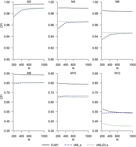The four indices shown are 1) the software-produced index ${\text{RMSEA}}_{\mathrm{D},\text{MV}};$ 2) the parallel uncorrected index ${\text{RMSEA}}_{\mathrm{D}};$ 3) the first proposed alternative, ${\text{RMSEA}}_{\text{cML},\mathrm{s}};$ and 4) the second proposed alternative, ${\text{RMSEA}}_{\text{cML}(\mathrm{D})}.$ Due to space limitations, results for even-numbered models only are shown. Figure 2 shows the parallel results for the CFI. These figures illustrate that existing DWLS indices tend to overestimate model fit. With the exception of the most mispecified model (M12), ${\text{RMSEA}}_{\mathrm{D}}$ and ${\text{RMSEA}}_{\mathrm{D},\text{MV}}$ are smaller than the ML RMSEA, and ${\text{CFI}}_{\mathrm{D}}$ and ${\text{CFI}}_{\mathrm{D},\text{MV}}$ are larger than the ML CFI. In the vast majority of conditions, ${\text{RMSEA}}_{\mathrm{D},\text{MV}}$ and ${\text{CFI}}_{\mathrm{D},\text{MV}}$ do better than the corresponding uncorrected DWLS indices ${\text{RMSEA}}_{\mathrm{D}}$ and ${\text{CFI}}_{\mathrm{D}},$ but they remain significantly biased. The underestimation of the ML RMSEA value by ${\text{RMSEA}}_{\mathrm{D},\text{MV}}$ is greatest when data are binary, and it becomes less pronounced with more categories, whereas the dependence on the number of categories is not as strong for ${\text{CFI}}_{\mathrm{D},\text{MV}}.$

Figure 1. Indices currently in use, ${\text{RMSEA}}_{\mathrm{D}}$ (Equation (8a)(8a) $${\text{RMSEA}}_{\mathrm{D}}=\sqrt{\frac{T_{\mathrm{D}}-df}{(N-1)df}}=\sqrt{\frac{{\widehat{F}}_{\mathrm{D}}}{df}-\frac{1}{N-1}}\to {\text{RMSEA}}_{\mathrm{D},0}=\sqrt{\frac{F_{\mathrm{D},0}}{df}}$$(8a) , black dot-dashed lines) and ${\text{RMSEA}}_{\mathrm{D},\text{MV}}$ (Equation (2a)(2a) $${\text{RMSEA}}_{\mathrm{D},\text{MV}}=\sqrt{\frac{T_{\mathrm{D},\text{MV}}-df}{(N-1)df}}=\sqrt{\frac{a{\widehat{F}}_{\mathrm{D}}}{df}+\frac{b/df-1}{N-1}}$$(2a) , black solid lines), as well as the two proposed solutions, ${\text{RMSEA}}_{\text{cML},\mathrm{s}}$ (Equation (5a)(5a) $${\text{RMSEA}}_{\text{cML},\mathrm{s}}=\sqrt{\frac{{\widehat{F}}_{\text{cML}}}{df}-\frac{k_{\text{cML}}}{df(N-1)}}$$(5a) , blue dashed lines) and ${\text{RMSEA}}_{\text{cML}(\mathrm{D}),\mathrm{s}}$ (Equation (6a)(6a) $${\text{RMSEA}}_{\text{cML}(\mathrm{D}),\mathrm{s}}=\sqrt{\frac{(N-1){\widehat{F}}_{\text{cML}(\mathrm{D})}}{(N-1)df}-\frac{k_{\text{cML}(\mathrm{D})}}{df(N-1)}}$$(6a) , green dotted lines). Where the green dotted lines are not visible, they overlap with the blue dashed lines. Sample size is N = 1000. Number of categories (2, 3, or 4) is on the x-axis. The y-axis range differs between the upper row and lower row. The flat gray line is the ML population RMSEA (see also Table 2).

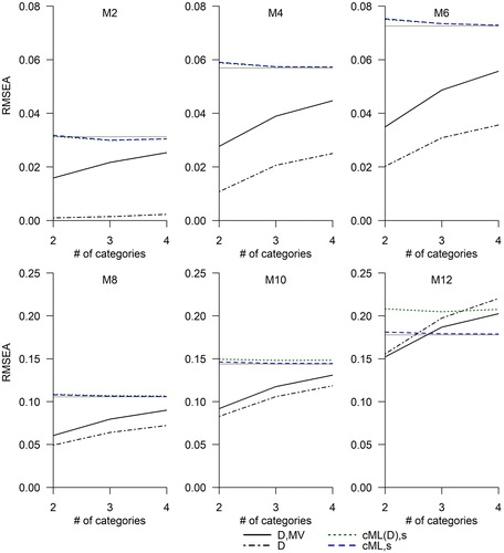
Figure 2. Indices currently in use, ${\text{CFI}}_{\mathrm{D}}$ (Equation (8b)(8b) $${\text{CFI}}_{\mathrm{D}}=1-\frac{T_{\mathrm{D}}-df}{T_{\mathrm{D},\mathrm{B}}-d{f}_{\mathrm{B}}}=\frac{{\widehat{F}}_{\mathrm{D}}-df/(N-1)}{{\widehat{F}}_{\mathrm{D},\mathrm{B}}-d{f}_{\mathrm{B}}/(N-1)}\to {\text{CFI}}_{\mathrm{D},0}=1-\frac{F_{\mathrm{D},0}}{F_{\mathrm{D},\mathrm{B},0}}$$(8b) , black dot-dashed lines) and ${\text{CFI}}_{\mathrm{D},\text{MV}}$ (Equation (2b)(2b) $${\text{CFI}}_{\mathrm{D},\text{MV}}=1-\frac{T_{\mathrm{D},\text{MV}}-df}{T_{\mathrm{D},\text{MV},\mathrm{B}}-d{f}_{\mathrm{B}}}=1-\frac{a{\widehat{F}}_{\mathrm{D}}+\frac{b-df}{N-1}}{a_{\mathrm{B}}{\widehat{F}}_{\mathrm{D},\mathrm{B}}+\frac{b_{\mathrm{B}}-d{f}_{\mathrm{B}}}{N-1}}$$(2b) , black solid lines), as well as two proposed solutions, ${\text{CFI}}_{\text{cML},\mathrm{s}}$ (Equation (5b)(5b) $${\text{CFI}}_{\text{cML},\mathrm{s}}=1-\frac{{\widehat{F}}_{\text{cML}}-k_{\text{cML}}/(N-1)}{{\widehat{F}}_{\text{cML},\mathrm{B}}-k_{\text{cML},\mathrm{B}}/(N-1)}.$$(5b) , blue dashed lines) and ${\text{CFI}}_{\text{cML}(\mathrm{D}),\mathrm{s}}$ (Equation (6b)(6b) $${\text{CFI}}_{\text{cML}(\mathrm{D}),\mathrm{s}}=1-\frac{{\widehat{F}}_{\text{cML}(\mathrm{D})}-k_{\text{cML}(\mathrm{D})}/(N-1)}{{\widehat{F}}_{\text{cML}(\mathrm{D}),\mathrm{B}}-k_{\text{cML}(\mathrm{D}),\mathrm{B}}/(N-1)},$$(6b) , green dotted lines). Where the green dotted lines are not visible, they overlap with the blue dashed lines. Sample size is N = 1000. Number of categories (2, 3, or 4) is on the x-axis. The y-axis range varies across the panels of the figure. The flat gray line is the ML population CFI (see also Table 2).

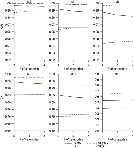
As a concrete example of how the use of existing DWLS fit indices may affect conclusions about the degree of misfit, consider the case when the population model is M8 and the data are binary. In this case, the ML values of RMSEA and CFI are .11 and .85, respectively (see Table 2). However, the average ${\text{RMSEA}}_{\mathrm{D},\text{MV}}$ is below .07 (see Figure 1) and the average ${\text{CFI}}_{\mathrm{D},\text{MV}}$ is almost .95 (see Figure 2). Applying the tentative cutoffs that many researchers use, the 1-factor model would likely be found well-fitting when using ${\text{RMSEA}}_{\mathrm{D},\text{MV}}$ and ${\text{CFI}}_{\mathrm{D},\text{MV}},$ whereas the ML fit index values suggest that the 1-factor model is actually quite a poor approximation to the structure of M8. On the other hand, ${\text{RMSEA}}_{\text{cML},\mathrm{s}}$ and ${\text{CFI}}_{\text{cML},\mathrm{s}},$ estimate the ML population values very well. This behavior is in line with theoretical expectations: These fit indices have the same population values as the ML fit indices. Any visible discrepancies, which are largest for binary data, are due to the remaining sampling fluctuations at N = 1000. Figures 1 and 2 also show that the average values of the DWLS approximations ${\text{RMSEA}}_{\text{cML}(\mathrm{D}),\mathrm{s}}$ and ${\text{CFI}}_{\text{cML}(\mathrm{D}),\mathrm{s}}$ are essentially identical to ${\text{RMSEA}}_{\text{cML},\mathrm{s}}$ and ${\text{CFI}}_{\text{cML},\mathrm{s}}$ for models that are not too misspecified (through M8). The approximation is worse but is still reasonable for M10 (for this model, the ML RMSEA and CFI are .144 and .713), but it fails for M12. However, when the misfit is as bad as it is for M12, the model is rejected using any fit index, existing or new.

Figures 3 and 4 illustrate the performance of fit indices in smaller samples. These figures only show the results for binary data. Figure 3 presents the average values of the currently used ${\text{RMSEA}}_{\mathrm{D},\text{MV}}$ and the proposed solutions ${\text{RMSEA}}_{\text{cML},\mathrm{s}}$ and ${\text{RMSEA}}_{\text{cML}(\mathrm{D}),\mathrm{s}}.$ The average value of ${\text{RMSEA}}_{\mathrm{D},\text{MV}}$ is much lower than the ML RMSEA and does not appear to vary much with sample size. On the other hand, ${\text{RMSEA}}_{\text{cML},\mathrm{s}}$ and ${\text{RMSEA}}_{\text{cML}(\mathrm{D}),\mathrm{s}}$ behave much more in line with how sample ML RMSEA estimates behave with continuous data (see, e.g., Brosseau-Liard et al., 2012), overestimating the population value in small samples, and approaching it from above as the sample size increases. The overestimation in small samples occurs partly because RMSEA is bounded below by zero, leading to bias in small samples, particularly when the true value is close to zero (i.e., for mildly misspecified models). At the smallest studied sample size (N = 200), this overestimation is quite severe, but it is greatly reduced by N = 400, and is negligible by N = 600. Overall, at N = 400 or greater, ${\text{RMSEA}}_{\text{cML},\mathrm{s}}$ and ${\text{RMSEA}}_{\text{cML}(\mathrm{D}),\mathrm{s}}$ produce less biased values than ${\text{RMSEA}}_{\mathrm{D},\text{MV}}.$ At N = 200, the degree of overestimation by ${\text{RMSEA}}_{\text{cML},\mathrm{s}}$ and ${\text{RMSEA}}_{\text{cML}(\mathrm{D}),\mathrm{s}}$ is similar, on average, to the degree of underestimation by ${\text{RMSEA}}_{\mathrm{D},\text{MV}},$ so that no index performs well. As was the case with N = 1000 (Figure 1), ${\text{RMSEA}}_{\text{cML}(\mathrm{D}),\mathrm{s}}$ is no longer a reasonable approximation to ${\text{RMSEA}}_{\text{cML},\mathrm{s}}$ for M12. For this population model, however, all fit indices would lead to the rejection of the 1-factor model: even ${\text{RMSEA}}_{\mathrm{D},\text{MV}}$ is above .14 in all samples.

Figure 3. Index currently in use, ${\text{RMSEA}}_{\mathrm{D},\text{MV}}$ (Equation (2a)(2a) $${\text{RMSEA}}_{\mathrm{D},\text{MV}}=\sqrt{\frac{T_{\mathrm{D},\text{MV}}-df}{(N-1)df}}=\sqrt{\frac{a{\widehat{F}}_{\mathrm{D}}}{df}+\frac{b/df-1}{N-1}}$$(2a) , black solid lines), as well as two proposed solutions, ${\text{RMSEA}}_{\text{cML},\mathrm{s}}$ (Equation (5a)(5a) $${\text{RMSEA}}_{\text{cML},\mathrm{s}}=\sqrt{\frac{{\widehat{F}}_{\text{cML}}}{df}-\frac{k_{\text{cML}}}{df(N-1)}}$$(5a) , blue dashed lines) and ${\text{RMSEA}}_{\text{cML}(\mathrm{D}),\mathrm{s}}$ (Equation (6a)(6a) $${\text{RMSEA}}_{\text{cML}(\mathrm{D}),\mathrm{s}}=\sqrt{\frac{(N-1){\widehat{F}}_{\text{cML}(\mathrm{D})}}{(N-1)df}-\frac{k_{\text{cML}(\mathrm{D})}}{df(N-1)}}$$(6a) , green dotted lines). Sample size is on the x-axis. Number of categories is 2. The y-axis range differs between the upper row and lower row. The flat gray line is the ML population RMSEA.

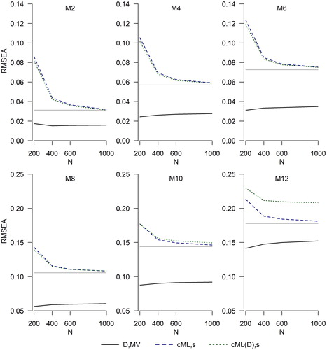
Figure 4. Index currently in use, ${\text{CFI}}_{\mathrm{D},\text{MV}}$ (Equation (2b)(2b) $${\text{CFI}}_{\mathrm{D},\text{MV}}=1-\frac{T_{\mathrm{D},\text{MV}}-df}{T_{\mathrm{D},\text{MV},\mathrm{B}}-d{f}_{\mathrm{B}}}=1-\frac{a{\widehat{F}}_{\mathrm{D}}+\frac{b-df}{N-1}}{a_{\mathrm{B}}{\widehat{F}}_{\mathrm{D},\mathrm{B}}+\frac{b_{\mathrm{B}}-d{f}_{\mathrm{B}}}{N-1}}$$(2b) , solid black lines), as well as two proposed solutions, ${\text{CFI}}_{\text{cML},\mathrm{s}}$ (Equation (5b)(5b) $${\text{CFI}}_{\text{cML},\mathrm{s}}=1-\frac{{\widehat{F}}_{\text{cML}}-k_{\text{cML}}/(N-1)}{{\widehat{F}}_{\text{cML},\mathrm{B}}-k_{\text{cML},\mathrm{B}}/(N-1)}.$$(5b) , blue dashed lines) and ${\text{CFI}}_{\text{cML}(\mathrm{D}),\mathrm{s}}$ (Equation (6b)(6b) $${\text{CFI}}_{\text{cML}(\mathrm{D}),\mathrm{s}}=1-\frac{{\widehat{F}}_{\text{cML}(\mathrm{D})}-k_{\text{cML}(\mathrm{D})}/(N-1)}{{\widehat{F}}_{\text{cML}(\mathrm{D}),\mathrm{B}}-k_{\text{cML}(\mathrm{D}),\mathrm{B}}/(N-1)},$$(6b) , green dotted lines). Sample size is on the x-axis. Number of categories is 2. The y-axis range differs between the upper row and lower row. The flat gray line is the ML population CFI.

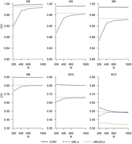
Figure 4 presents the parallel results for the CFI. The pattern here is very similar. ${\text{CFI}}_{\text{cML},\mathrm{s}}$ and ${\text{CFI}}_{\text{cML}(\mathrm{D}),\mathrm{s}}$ outperform ${\text{CFI}}_{\mathrm{D},\text{MV}}$ in nearly all conditions at N = 400 and N = 600. At N = 200, the results are mixed, with ${\text{CFI}}_{\mathrm{D},\text{MV}}$ severely overestimating the ML population value and the new fit indices severely underestimating it. The case of M12 is curious: here, ${\text{CFI}}_{\mathrm{D},\text{MV}}$ appears to estimate the ML population values more closely, but this is pure coincidence. Overall, Figures 3 and 4 reveal that no fit index is able to accurately evaluate model fit with binary data at N = 200. Larger samples are needed with such data to reliably gauge model fit.

Figures 5 and 6 present parallel results to Figures 3 and 4 for 3-category data. Figure 5 shows that for nearly all models and sample sizes, ${\text{RMSEA}}_{\text{cML},\mathrm{s}}$ and ${\text{RMSEA}}_{\text{cML}(\mathrm{D}),\mathrm{s}}$ outperform ${\text{RMSEA}}_{\mathrm{D},\text{MV}}.$ They also exhibit very little bias, even at N = 200. The only exception is the most misspecified model, M12, where the approximation ${\text{RMSEA}}_{\text{cML}(\mathrm{D}),\mathrm{s}}$ again fails. Figure 6 shows a similar pattern of results for the CFI. As with binary data, for M12, ${\text{CFI}}_{\mathrm{D},\text{MV}}$ happens to produce similar values to ML values. The results for 4 categories are similar and are omitted to save space. Overall, the new fit indices outperform the indices currently in use in samples of N = 400 and higher with binary data, and in all samples with 3- and 4-category data.

Figure 5. Index currently in use, ${\text{RMSEA}}_{\mathrm{D},\text{MV}}$ (Equation (2a)(2a) $${\text{RMSEA}}_{\mathrm{D},\text{MV}}=\sqrt{\frac{T_{\mathrm{D},\text{MV}}-df}{(N-1)df}}=\sqrt{\frac{a{\widehat{F}}_{\mathrm{D}}}{df}+\frac{b/df-1}{N-1}}$$(2a) , black solid lines), as well as two proposed solutions, ${\text{RMSEA}}_{\text{cML},\mathrm{s}}$ (Equation (5a)(5a) $${\text{RMSEA}}_{\text{cML},\mathrm{s}}=\sqrt{\frac{{\widehat{F}}_{\text{cML}}}{df}-\frac{k_{\text{cML}}}{df(N-1)}}$$(5a) , blue dashed lines) and ${\text{RMSEA}}_{\text{cML}(\mathrm{D}),\mathrm{s}}$ (Equation (6a)(6a) $${\text{RMSEA}}_{\text{cML}(\mathrm{D}),\mathrm{s}}=\sqrt{\frac{(N-1){\widehat{F}}_{\text{cML}(\mathrm{D})}}{(N-1)df}-\frac{k_{\text{cML}(\mathrm{D})}}{df(N-1)}}$$(6a) , green dotted lines). Sample size is on the x-axis. Number of categories is 3. The y-axis range differs between the upper row and lower row. The flat gray line is the ML population RMSEA.

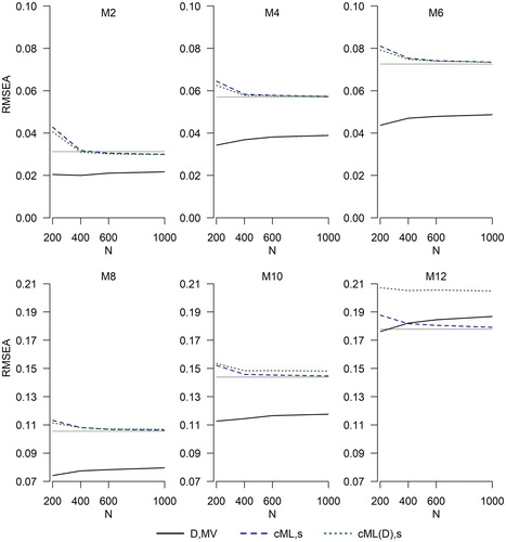
Figure 6. Index currently in use, ${\text{CFI}}_{\mathrm{D},\text{MV}}$ (Equation (2b)(2b) $${\text{CFI}}_{\mathrm{D},\text{MV}}=1-\frac{T_{\mathrm{D},\text{MV}}-df}{T_{\mathrm{D},\text{MV},\mathrm{B}}-d{f}_{\mathrm{B}}}=1-\frac{a{\widehat{F}}_{\mathrm{D}}+\frac{b-df}{N-1}}{a_{\mathrm{B}}{\widehat{F}}_{\mathrm{D},\mathrm{B}}+\frac{b_{\mathrm{B}}-d{f}_{\mathrm{B}}}{N-1}}$$(2b) , black solid lines), as well as two proposed solutions, ${\text{CFI}}_{\text{cML},\mathrm{s}}$ (Equation (5b)(5b) $${\text{CFI}}_{\text{cML},\mathrm{s}}=1-\frac{{\widehat{F}}_{\text{cML}}-k_{\text{cML}}/(N-1)}{{\widehat{F}}_{\text{cML},\mathrm{B}}-k_{\text{cML},\mathrm{B}}/(N-1)}.$$(5b) , blue dashed lines) and ${\text{CFI}}_{\text{cML}(\mathrm{D}),\mathrm{s}}$ (6b, green dotted lines). Sample size is on the x-axis. Number of categories is 3. The y-axis range differs between the upper row and lower row. The flat gray line is the ML population CFI.

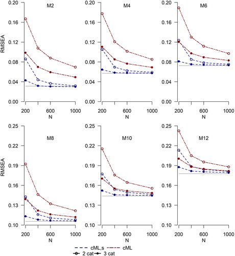
Figure 7 illustrates why small-sample robustification with scaling constants is necessary to produce better performance of the new fit indices. To save space, I focus on the cML RMSEA. The pattern of results for the DWLS approximation and for the CFI under both solutions is the same. In this figure, average values of ${\text{RMSEA}}_{\text{cML},\mathrm{s}}$ and ${\text{RMSEA}}_{\text{cML}}$ are shown for 2- and 3-category data. The bias in ${\text{RMSEA}}_{\text{cML}}$ is quite large relative to ${\text{RMSEA}}_{\text{cML},\mathrm{s}},$ and this bias is not negligible even at N = 1000. This finding is important because the uncorrected fit indices in Equations (9a)(9a) $${\text{RMSEA}}_{\text{cML}}=\sqrt{\frac{(N-1){\widehat{F}}_{\text{cML}}-df}{(N-1)df}}$$(9a) and (9b)(9b) $${\text{CFI}}_{\text{cML}}=1-\frac{(N-1){\widehat{F}}_{\text{cML}}-df}{(N-1){\widehat{F}}_{\text{cML},\mathrm{B}}-d{f}_{\mathrm{B}}}$$(9b) are easier to compute; all that is needed is the minimum (or approximate minimum) of the cML fit function. However, these uncorrected indices can be quite biased.

Figure 7. Average values of cML RMSEA with and without robustification: ${\text{RMSEA}}_{\text{cML},\mathrm{s}}$ (Equation (5a)(5a) $${\text{RMSEA}}_{\text{cML},\mathrm{s}}=\sqrt{\frac{{\widehat{F}}_{\text{cML}}}{df}-\frac{k_{\text{cML}}}{df(N-1)}}$$(5a) ; blue dashed lines) and ${\text{RMSEA}}_{\text{cML}}$ (Equation (9a)(9a) $${\text{RMSEA}}_{\text{cML}}=\sqrt{\frac{(N-1){\widehat{F}}_{\text{cML}}-df}{(N-1)df}}$$(9a) ; red dot-dashed lines). Sample size is on the x-axis. Number of categories is 2 (empty circles) or 3 (filled circles). The y-axis range differs between the upper row and lower row. The flat gray line is the ML population RMSEA.

Figures 1 to 7 presented only the average values of the fit indices across all replications. Supplementary files posted on OSF contain a host of other measures, such as empirical standard deviations, coverage of approximate 90% confidence intervals (CIs; see Appendix), average CI width, and so on. These results were examined to safeguard against any unusual possibilities (e.g., that the new fit indices are more variable while being on average relatively unbiased). However, none of these additional measures indicated any problems with the newly proposed solutions, so they are are not presented. The two solutions perform very similarly on the additional measures, and there is no unusual variability. Coverage results are sometimes poor (e.g., when N = 200 with binary data), as is common for RMSEA in small samples, but in most conditions where the new fit indices show little bias coverage results are also good. None of the additional measures reveal any advantages of the old fit indices over the new fit indices.

Lastly, a reviewer suggested the possibility that the quality of the DWLS approximation to cML may depend on the thresholds used for categorization. This is because the asymptotic values of the diagonals of the DWLS weight matrix (i.e., D) are dependent on the thresholds (Xia & Yang, 2018). When the model is wrong, the magnitude of the difference between DWLS and cML parameter estimates will be partly a function of the thresholds. To put this theory to a test, I included two additional threshold conditions for binary data: all thresholds set to 0 and all thresholds set to 1.5. The latter condition is very extreme: it means that each item on the scale is endorsed by fewer than 7% of participants. Because very little information is available about model parameters in such a case, N = 1000 was not sufficient to compare asymptotic values, and I increased the sample size to N = 5000. The results are shown in Table 3. The differences between the cML and the DWLS approximation fit indices do not vary very much across the three threshold conditions, except for M12, where in the extreme thresholds condition the differences are larger.

Table 3. Average values of the new fit indices across 1000 replications, with binary data and under three different choices of thresholds, N = 5000.

Thresholds	Model	${\text{RMSEA}}_{\text{cML}(\mathrm{D}),\mathrm{s}}$	${\text{RMSEA}}_{\text{cML},\mathrm{s}}$	${\text{CFI}}_{\text{cML}(\mathrm{D}),\mathrm{s}}$	${\text{CFI}}_{\text{cML},\mathrm{s}}$
Original	M2	0.031	0.031	0.989	0.989
All 0	M2	0.031	0.031	0.989	0.989
All 1.5	M2	0.031	0.031	0.988	0.988
Original	M4	0.057	0.057	0.966	0.966
All 0	M4	0.057	0.057	0.966	0.966
All 1.5	M4	0.058	0.058	0.965	0.965
Original	M6	0.073	0.073	0.946	0.946
All 0	M6	0.073	0.073	0.946	0.946
All 1.5	M6	0.075	0.075	0.943	0.943
Original	M8	0.107	0.106	0.851	0.853
All 0	M8	0.107	0.106	0.850	0.853
All 1.5	M8	0.109	0.108	0.848	0.850
Original	M10	0.148	0.144	0.697	0.713
All 0	M10	0.148	0.144	0.697	0.713
All 1.5	M10	0.150	0.146	0.694	0.711
Original	M12	0.208	0.179	0.375	0.540
All 0	M12	0.208	0.178	0.374	0.540
All 1.5	M12	0.221	0.182	0.316	0.538

Discussion

Summary and recommendations

Researchers who fit SEMs to categorical data rely on software defaults for the computations of indices of approximate fit, such as RMSEA and CFI. When data are categorical, the most frequently used limited information estimation method is DWLS. It is the default in Mplus and lavaan, and an option in other packages such as LISREL. However, these software programs compute categorical fit indices by simply replacing the chi-square statistic $T_{\text{ML}}$ with a DWLS categorical test statistic, such as $T_{\mathrm{D},\text{MV}},$ in the ML equations. Recently, methodologists have begun pointing out that the resulting fit indices have poor properties (Monroe & Cai, 2015; Xia & Yang, 2018, 2019). Specifically, indices obtained in this way tend to indicate much better model fit than what would have been the case had the data been continuous. Uncritical interpretation of these fit indices in the same way as would be done with continuous normal data can have serious consequences for the researchers’ ability to detect model misfit.

This article proposed two solutions, which involve replacing the DWLS fit function minimum with the cML fit function minimum (Solution 1) or with its approximation using DWLS parameter estimates (Solution 2). Additional robustification is applied to both solutions by replacing the degrees of freedom with the correct expected value of the uncorrected test statistic (Brosseau-Liard et al., 2012; Brosseau-Liard & Savalei, 2014). The population values of the resulting fit indices are equal to the population ML fit index values (Solution 1) or are approximations of it for models that are not seriously misspecified (Solution 2). Thus, the proposed solutions result in fit indices that mimic the values that would have been obtained had the data not been categorized. The impact of the loss of information due to discretization is on the precision of these estimates (relative to continuous data), not on their asymptotic expected values.

The results of the simulation study designed to demonstrate the superiority of the proposed solutions over the existing computations were in line with the theoretical expectations. The fit indices currently in use, ${\text{RMSEA}}_{\mathrm{D},\text{MV}}$ and ${\text{CFI}}_{\mathrm{D},\text{MV}},$ overestimated model fit in most conditions. This distortion was greatest for binary data. Theoretically, ${\text{RMSEA}}_{\mathrm{D},\text{MV}}$ and ${\text{CFI}}_{\mathrm{D},\text{MV}}$ will remain biased estimates of the ML fit indices even if the data have a very high number of categories, because the general form of the fit function remains misspecified. In contrast, both proposed solutions performed well across most population models with sample sizes of N = 400 or greater, essentially always outperforming indices currently in use. The proposed solutions also performed well at N = 200 with 3- and 4-category data. With N = 200 and binary data, all fit indices, existing and new, did poorly, suggesting that this may not be a sufficient sample size to estimate the degree of misfit when data are so severely categorized. Future research should also explore if better small-sample corrections for the proposed indices may exist.

The DWLS approximation (Solution 2) performed well for models with $\text{RMSEA}\le .14$ and $\text{CFI}\ge .71.$ For the population models where the misfit of the 1-factor model was worse than these values, the DWLS approximation began to diverge considerably from cML (Solution 1). However, in these cases, all fit indices indicated such bad fit that researchers’ conclusions would be unaffected by the choice of the fit index. Thus, I do not view the deterioration of the DWLS approximation in such cases as problematic, and I recommend the cML and the DWLS approximations equally. The advantage of the DWLS approximation is that it allows researchers to continue to use the familiar DWLS estimator with categorical data. The advantage of the cML solution is that even the uncorrected fit indices are always consistent for the ML population values (see Equations (9a)(9a) $${\text{RMSEA}}_{\text{cML}}=\sqrt{\frac{(N-1){\widehat{F}}_{\text{cML}}-df}{(N-1)df}}$$(9a) and (9b)(9b) $${\text{CFI}}_{\text{cML}}=1-\frac{(N-1){\widehat{F}}_{\text{cML}}-df}{(N-1){\widehat{F}}_{\text{cML},\mathrm{B}}-d{f}_{\mathrm{B}}}$$(9b) ), and the small-sample robustification corrections are more straight-forward to compute, because the formulae are identical to the scaling constants used to obtain the M chi-square.

Limitations and future directions

Both proposed solutions have a drawback, which is that the cML fit function cannot be evaluated when the input matrix is non-pd. The matrix of polychoric correlations is estimated bivariately in most software packages, which can lead to non-pd estimates in smaller samples, particularly for binary data with extreme thresholds. In their comprehensive simulations, Yang-Wallentin et al. (2010) found that non-pd matrices occurred only in 7–9% of replications at N = 100. In the simulation study reported here, non-pd matrices occurred in about 5% of the replications at N = 200 with binary data.¹¹ Smoothing algorithms for non-pd matrices may be considered in the situation where non-pd matrices occur (e.g., Bentler & Yuan, 2011; Yuan & Chan, 2011; Yuan & Chan, 2008), though empirical evidence that these methods produce quality estimates is mixed (Debelak & Tran, 2016; Kracht & Waller, 2018). However, it is worth noting that the non-pd matrices occurred in precisely the same conditions where all categorical fit indices (old and new) were significantly biased (N = 200, binary data). Thus, it can be argued that the occurrence of non-pd matrices can be interpreted as a sign that there is not enough information in the data about the model (see also Yang-Wallentin et al., 2010). Rules of thumb for SEM generally suggest at least 200 cases (Kline, 2016), but with certain types of categorical data minimal sample size requirements may need to be higher.

In this study I have focused on two commonly used fit indices: RMSEA and CFI. The extension of the ideas in this article to many other fit indices would follow the same logic. For example, another comparative fit index printed by both Mplus and lavaan is TLI, whose ML population value can be expressed in terms of the ML CFI population value as follows: ${\text{TLI}}_{\text{ML},0}=1-\frac{d{f}_{\mathrm{B}}}{df}(1-{\text{CFI}}_{\text{ML},0}).$ Substituting ${\text{CFI}}_{\text{cML}(\mathrm{D}),\mathrm{s}}$ or ${\text{CFI}}_{\text{cML},\mathrm{s}}$ into this equation would yield an estimate of the population ML TLI obtained from categorical data. This estimate changes the sample TLI definition to involve the subtraction of the expected values from the test statistics. At the same time, not all fit indices would require corrections of the type proposed in this article. The standardized root mean square residual (SRMR), which is the square-root of the average squared difference between the model-implied and the observed correlations, does not depend on the fit function minimum; thus, this index can be computed and interpreted in the same way with continuous and categorical data. Because the model-implied correlations will be different when estimated using DWLS versus cML, the population SRMR values will be different for DWLS versus cML estimation, but these differences are expected to be small unless the model is extremely misspecified (the magnitude of the differences should be similar to those of Solution 1 versus Solution 2).

A limitation of the simulation study presented in this article is that the same 1-factor model was always fit to data generated from 1- and 2-factor populations. Future research should expand these simulations to investigate the performance of the proposed fit indices under other population and fitted models. However, this limitation is not as serious as may appear at first glance because what matters for the study of the behavior of approximate fit indices is not the precise true model and the precise hypothesized model, but the resulting amount of misspecification on the RMSEA and CFI metric. In this study, the degree of misspecification varied considerably across the twelve population models (see Table 2). In addition, the proposed fit indices have theoretical advantages of approaching or approximating their continuous data ML counterparts, and the simulation study serves a more limited goal of providing an empirical illustration of these theoretical advantages.

In the simulation results reported in this article, I focused on the DWLS estimator because it is the default estimator in Mplus and lavaan. However, the ULS estimator is a special case of DWLS with D = I. All the simulation conditions were analyzed using ULS as well; the results are similar and are available on OSF. Future research should tackle how to extend the ideas in this article to other categorical data approaches. For methods based on the polychoric correlations, such as DWLS and ULS, constructing categorical fit indices to approximate the ML fit indices makes particular sense because polychoric correlations approach Pearson correlations among the underlying continuous variables as the sample size increases. But not all categorical SEM methods fit the model to the polychoric correlations. Some limited information categorical SEM methods directly model the m-way contingency tables of categorical data (Maydeu-Olivares & Joe, 2005; Monroe & Cai, 2015). Full information categorical estimation methods that are used in item response theory (IRT) model the entire multinomial distribution of the data. For these types of estimators, misfit measures such as the RMSEA can be defined on the metric of the ordinal data (rather than transforming to polychoric correlations), and it may be that they are more appropriate. However, if these indices are used with cutoffs, they would require the development of new guidelines. Currently, approximate fit indices in IRT applications are compared to benchmarks developed for fit indices in the context of continuous normal data, creating the same problem of interpretation (Monroe & Cai, 2015). It may be that there is room for fit indices as defined in this article to be used alongside existing versions of categorical fit indices with estimators that are not based on polychoric correlations; reference to a single common metric may be useful for applied researchers, and the indices proposed here can communicate additional useful information.

The counterargument to the proposals in this article is that categorical fit indices should not have to agree with their continuous counterparts. By this argument, categorical data contain less information about model misfit because of loss of information due to discretization, and thus the same misspecified model should fit better when data are categorical. Just like the test statistic loses power when the data become categorical or nonnormal, so should fit indices. However, while the MV chi-square regains power as the sample size increases, currently used fit indices ${\text{RMSEA}}_{\mathrm{D},\text{MV}}$ and ${\text{CFI}}_{\mathrm{D},\text{MV}}$ continue to measure misfit on a different metric and thus would require different benchmarks and extensive further study before their meaning can be calibrated. Further, their population values depend on variables such as the particular estimator used (DWLS vs. ULS), the number of categories in the data, and the values of the thresholds (Xia & Yang, 2018, 2019), complicating the provision of guidelines further. A similar problem occurs in the context of nonnormal data, where simply substituting M or MV test statistics to obtain fit indices creates the ironic situation whereby the model appears to fit better with increasing nonnormality; the proposed solutions are similar (Brosseau-Liard et al., 2012; Brosseau-Liard & Savalei, 2014). The same problem also occurs with incomplete data (Zhang & Savalei, 2019). Investigating the behavior of fit indices under these various situations and their intersections in order to provide guidelines for researchers may be prohibitive. In this article I argue that it may be more practical and useful for applied researchers to redefine fit index computations so that they estimate misfit assuming data are complete, continuous, and normally distributed.

In making the arguments in this article, I certainly do not intend to imply that fit indices have unambiguous interpretations even with continuous normal data, or that everyone agrees on what the cutoffs should be (or whether there should even be cutoffs). In fact, in the case of the RMSEA, I have contributed to the argument against firm cutoffs myself (Savalei, 2012). However, there is no denying that fit indices are at present the primary way in which researchers gauge model fit, and that many researchers rely on cutoffs. While methodological work can help researchers do so in a more justified and nuanced way, doing so is made more difficult if the population values of the fit indices change depending on the estimation method and type of data. Ultimately, the developments proposed in this article will lead to improved research practices by unifying decision-making using fit indices across different types of data.

Article information

Conflict of interest disclosures: Each author signed a form for disclosure of potential conflicts of interest. No authors reported any financial or other conflicts of interest in relation to the work described.

Ethical principles: The authors affirm having followed professional ethical guidelines in preparing this work. These guidelines include obtaining informed consent from human participants, maintaining ethical treatment and respect for the rights of human or animal participants, and ensuring the privacy of participants and their data, such as ensuring that individual participants cannot be identified in reported results or from publicly available original or archival data.

Funding: This work was not supported.

Role of the funders/sponsors: None of the funders or sponsors of this research had any role in the design and conduct of the study; collection, management, analysis, and interpretation of data; preparation, review, or approval of the manuscript; or decision to submit the manuscript for publication.

Acknowledgments: The ideas and opinions expressed herein are those of the authors alone, and endorsement by the author’s institution is not intended and should not be inferred.

Notes

1 In rare cases where $T_{\text{ML}}<df,$ the sample RMSEA is set to 0. Similarly, the value of the sample CFI is rounded to fall within the [0,1] interval. These bounds are omitted from Equations (1a) and (1b) and all future equations for readability.

2 The shift constants $b$ and $b_{\mathrm{B}}$ disappear asymptotically.

3 Of course, assumptions must be met, such as multivariate normality of the underlying continuous variables.

4 Parameter estimates will also slightly differ, unless the model is exactly true (for a theoretical analysis of this problem, see Olsson, Foss, Troye, & Howell, 2000; Yuan & Chan, 2005). However, as will be shown later in this article, the discrepancy in the parameter estimates has a much smaller effect on the fit indices than the discrepancy in the fit functions.

5 In lavaan, cML estimates can be obtained by specifying a custom weight matrix. However, this procedure does not produce correct standard errors or test statistics without additional special programming.

6 Some readers may question whether minimizing the ML fit function with the correlation matrix as input is the same as “ML”. However, the underlying continuous variables are unobserved and their variances can be arbitrarily set to 1. In other words, in the single-group context, we are only able to fit models to categorized data that do not place any constraints on the variances (Shapiro & Browne, 1990).

7 The only correctly specified fit function with polychoric correlations is “WLS” (see Table 1), which correctly takes the variability of polychoric correlations into account, but this estimation method does not perform well unless the sample size is very large (Muthén et al., 1997).

8 The following identity holds: ${\tilde{D}}_p=D_{p}D{\prime }_p\tilde{L}\prime ,$ where $\tilde{L}$ is a $.5p(p-1)\times p^2$ elimination matrix defined in Schott (2016).

9 I would like to thank Steve Reise for providing parameter estimates from this dataset.

10 The exact threshold values were .608, −.632, .261, .282, .434, −.123, .159, .305, .171, −.117, .524, .743, and .227.

11 To demonstrate the impact of extreme thresholds, I extended the condition in which all thresholds are 1.5 (introduced in Table 3 for N = 5000) to smaller sample sizes. For M3 (an arbitrary representative model), the number of replications in which the new fit indices could be computed was 1, 206, 736, and 996 for the sample sizes of N = 200, 400, 600, and 1000, respectively. However, this condition is unrealistic as it represents a 13-item scale where only 7% of the sample endorse each item.

Appendix:

Additional details for Equations 6a and 6b

From asymptotic theory (e.g., Shapiro, 2007), we have that $\sqrt{N}(r-{\widehat{\rho }}_{\mathrm{D}})\approx \sqrt{N}{D}_0{U}_0(r-r_0).$ Even though ${\widehat{\theta }}_{\mathrm{D}}$ does not minimize $F_{\text{cML}},$ when the model is correct we can approximate ${\widehat{F}}_{\text{cML}(\mathrm{D})}\approx (r-{\widehat{\rho }}_{\mathrm{D}})\prime W_0(r-{\widehat{\rho }}_{\mathrm{D}})\approx (r-r_0)\prime U_0{D}_0{W}_0{D}_0{U}_0(r-r_0),$ where W₀ is the population limit of $W_{\text{cML}(\mathrm{D})}.$ Using the output of DWLS estimation, the distribution of $T_{\text{cML}(\mathrm{D})}=(N-1)F_{\text{cML}}({\widehat{\theta }}_{\mathrm{D}})$ can be approximated by a mixture of independent 1 degree of freedom chi-squares with eigenvalues of $U_{\mathrm{D}}D{W}_{\text{cML}(\mathrm{D})}D{U}_{\mathrm{D}}\Gamma$ as the weights, and the approximate expected value of $T_{\text{cML}(\mathrm{D})}$ is given by $k_{\text{cML}(\mathrm{D})}=tr\left\{U_{\mathrm{D}}D{W}_{\text{cML}(\mathrm{D})}D{U}_{\mathrm{D}}\Gamma \right\}.$

An approximate CI for ${\text{RMSEA}}_{ML(D),s}$ can also be computed. We need an approximate chi-square test statistic. We will use the M chi-square $T_{\mathit{cML}(D),M}=\frac{df}{k_{\text{cML}(\mathrm{D})}}{T}_{\text{cML}(\mathrm{D})}.$ Then, following the procedure of Browne and Cudeck (1992), let ${\widehat{\lambda }}_{M,.05}$ and ${\widehat{\lambda }}_{M,.95}$ be such that $T_{\mathit{cML}(D),M}$ is the 5th percentile of ${\chi }^2(df,{\widehat{\lambda }}_{M,.05})$ and the 95th percentile of ${\chi }^2(df,{\widehat{\lambda }}_{M,.95}).$ Then, $L=\frac{k_{\text{cML}(\mathrm{D})}}{df}{\widehat{\lambda }}_{M,.05},U=\frac{k_{\text{cML}(\mathrm{D})}}{df}{\widehat{\lambda }}_{M,.95},$ and the approximate 90% CI is given by $$\sqrt{\max \left(0,\frac{L}{(N-1)df}\right)},\sqrt{\max \left(0,\frac{U}{(N-1)df}\right)}$$

See Savalei (2018) for how to compute approximate CIs based on the MV chi-square instead.

References

- Asparouhov, T., & Muthén, B. (2010). Simple second order chi-square correction. https://www.statmodel.com/download/WLSMV_new_chi21.pdf.
- Bentler, P. M. (1990). Comparative fit indexes in structural models. Psychological Bulletin, 107(2), 238–246. doi:10.1037/0033-2909.107.2.238
- Bentler, P. M. (2008). EQS structural equation modeling software. Encino, CA: Multivariate Software.
- Bentler, P. M., & Yuan, K.-H. (2011). Positive definiteness via off-diagonal scaling of a symmetric indefinite matrix. Psychometrika, 76(1), 119–123. doi:10.1007/s11336-010-9191-3
- Bollen, K. A. (1989). Structural equations with latent variables. New York, NY: Wiley.
- Brosseau-Liard, P., & Savalei, V. (2014). Adjusting relative fit indices for nonnormality. Multivariate Behavioral Research, 49(5), 460–470. doi:10.1080/00273171.2014.933697
- Brosseau-Liard, P., Savalei, V., & Li, L. (2012). An investigation of the sample performance of two non-normality corrections for RMSEA. Multivariate Behavioral Research, 47(6), 904–930. doi:10.1080/00273171.2012.715252
- Browne, M. W., & Cudeck, R. (1992). Alternative ways of assessing model fit. Sociological Methods & Research, 21, 230–258. doi:10.1177/0049124192021002005
- Debelak, R., & Tran, U. S. (2016). Comparing the effects of different smoothing algorithms on the assessment of dimensionality of ordered categorical items with parallel analysis. PLoS One, 11(2), e0148143. doi:10.1371/journal.pone.0148143
- Hu, L., & Bentler, P. M. (1999). Cutoff criteria for fit indexes in covariance structure analysis: Conventional criteria versus new alternatives. Structural Equation Modeling: A Multidisciplinary Journal, 6(1), 1–55. doi:10.1080/10705519909540118
- Jöreskog, K., & Sörbom, D. (1996). LISREL 8: User’s reference guide. Scientific Software International. Retrieved from https://books.google.ca/books?id=9AC-s50RjacC.
- Kenny, D. A., & McCoach, D. B. (2003). Effect of the number of variables on measures of fit in structural equation modeling. Structural Equation Modeling: A Multidisciplinary Journal, 10(3), 333–351. doi:10.1207/S15328007SEM1003_1
- Kline, R. B. (2016). Principles and practice of structural equation modeling (4th ed.). New York, NY: Guilford Press.
- Kracht, J., & Waller, N. G. (2018). A comparison of matrix smoothing algorithms. Multivariate Behavioral Research, 53(1), 136–137. doi:10.1080/00273171.2017.1404899
- Magnus, J. R., & Neudecker, H. (1999). Matrix differential calculus with applications in statistics and econometrics (2nd ed.). New York, NY: Wiley.
- Maydeu-Olivares, A., & Joe, H. (2005). Limited- and full-information estimation and goodness-of-fit testing in 2n contingency tables: A unified framework. Journal of the American Statistical Association, 100(471), 1009–1020. doi:10.1198/016214504000002069
- McDonald, R. P., & Ho, M.-H R. (2002). Principles and practice in reporting structural equation analyses. Psychological Methods, 7(1), 64–82. doi:10.1037/1082-989X.7.1.64
- McNeish, D., An, J., & Hancock, G. R. (2018). The thorny relation between measurement quality and fit index cutoffs in latent variable models. Journal of Personality Assessment, 100(1), 43–52. doi:10.1080/00223891.2017.1281286
- Miles, J., & Shevlin, M. (2007). A time and a place for incremental fit indices. Personality and Individual Differences, 42(5), 869–874. doi:10.1016/j.paid.2006.09.022
- Monroe, S., & Cai, L. (2015). Evaluating structural equation models for categorical outcomes: A new test statistic and a practical challenge of interpretation. Multivariate Behavioral Research, 50(6), 569–583. doi:10.1080/00273171.2015.1032398
- Muthén, B. (1993). Goodness of fit with categorical and other nonnormal variables. In K. A. Bollen & J. S. Long (Eds.), Testing structural equation models (pp. 205–234). Newbury Park, CA: Sage.
- Muthén, B., Toit, S. H. C. d., & Spisic, D. (1997). Robust inference using weighted least squares and quadratic estimating equations in latent variable modeling with categorical and continuous outcomes. Unpublished Manuscript. Retrieved from https://www.statmodel.com/download/Article_075.pdf.
- Muthén, L. K., & Muthén, B. O. (2017). Mplus user’s guide (8th ed.). Los Angeles, CA: Muthén and Muthén. Retrieved from https://www.statmodel.com/download/usersguide/MplusUserGuideVer_8.pdf.
- Ogasawara, H. (2001). Approximations to the distributions of fit indexes for misspecified structural equation models. Structural Equation Modeling: A Multidisciplinary Journal, 8(4), 556–574. doi:10.1207/S15328007SEM0804_03
- Olsson, U., Foss, T., Troye, S., & Howell, R. (2000). The performance of ML, GLS, and WLS estimation in structural equation modeling under conditions of misspecification and nonnormality. Structural Equation Modeling: A Multidisciplinary Journal, 7(4), 557–595. doi:10.1037/1082-989X.1.1.16
- R Core Team. (2019). R: A language and environment for statistical computing. Computer software manual. Vienna, Austria. Retrieved from https://www.R-project.org/.
- Rhemtulla, M., Brosseau-Liard, P., & Savalei, V. (2012). How many categories is enough to treat data as continuous? A comparison of robust continuous and categorical SEM estimation methods under a range of non-ideal situations. Psychological Methods, 17(3), 354–373. doi:10.1037/a0029315
- Rosseel, Y. (2012). lavaan: An R package for structural equation modeling. Journal of Statistical Software, 48(2), 1–36. doi:10.18637/jss.v048.i02
- Saris, W. E., Satorra, A., & Veld, W. M. V. d. (2009). Testing structural equation models or detection of misspecifications? Structural Equation Modeling: A Multidisciplinary Journal, 16(4), 561–582. doi:10.1080/10705510903203433
- Savalei, V. (2012). The relationship between root mean square error of approximation and model misspecification in confirmatory factor analysis models. Educational and Psychological Measurement, 72(6), 910–932. doi:10.1177/0013164412452564
- Savalei, V. (2014). Understanding robust corrections in structural equation modeling. Structural Equation Modeling: A Multidisciplinary Journal, 21(1), 149–160. doi:10.1080/10705511.2013.824793
- Savalei, V. (2018). On the computation of the RMSEA and CFI from the mean-and-variance corrected test statistic with nonnormal data in SEM. Multivariate Behavioral Research, 53(3), 419–429. doi:10.1080/00273171.2018.1455142
- Schott, J. R. (2016). Matrix analysis for statistics (3rd ed.). Hoboken, NJ: Wiley.
- Shapiro, A. (2007). Statistical inference of moment structures. In S.-Y. L. Lee (Ed.), Handbook of latent variable and related models (pp. 229–260). Amsterdam, Netherlands: Elsevier.
- Shapiro, A., & Browne, M. (1990). On the treatment of correlation structures as covariance structures. Linear Algebra and Its Applications, 127, 567–587. doi:10.1016/0024-3795(90)90362-G
- Shi, D., Lee, T., & Maydeu-Olivares, A. (2019). Understanding the model size effect on SEM fit indices. Educational and Psychological Measurement, 79(2), 310–334. doi:10.1177/0013164418783530
- Steiger, J. H. (1990). Structural model evaluation and modification: An interval estimation approach. Multivariate Behavioral Research, 25(2), 173–180. doi:10.1207/s15327906mbr2502_4
- Xia, Y., & Yang, Y. (2018). The influence of number of categories and threshold values on fit indices in structural equation modeling with ordered categorical data. Multivariate Behavioral Research, 53(5), 731–755. doi:10.1080//00273171.2018.1480346
- Xia, Y., & Yang, Y. (2019). RMSEA, CFI, and TLI in structural equation modeling with ordered categorical data: The story they tell depends on the estimation methods. Behavior Research Methods, 51(1), 409–428. doi:10.3758/s13428-018-1055-2
- Yang-Wallentin, F., Jöreskog, K. G., & Luo, H. (2010). Confirmatory factor analysis of ordinal variables with misspecified models. Structural Equation Modeling: A Multidisciplinary Journal, 17(3), 392–423. doi:10.1080/10705511.2010.489003
- Yuan, K.-H., & Chan, W. (2005). On nonequivalence of several procedures of structural equation modeling. Psychometrika, 70(4), 791–798. doi:10.1007/s11336-001-0930-9
- Yuan, K.-H., & Chan, W. (2008). Structural equation modeling with near singular covariance matrices. Computational Statistics & Data Analysis, 52(10), 4842–4858. doi:10.1016/j.csda.2008.03.030
- Zhang, X., & Savalei, V. (2019). Examining the effect of missing data on RMSEA and CFI under normal theory full-information maximum likelihood. Structural Equation Modeling: A Multidisciplinary Journal. doi:10.1080/10705511.2019.1642111