Bayesian Testing of Scientific Expectations under Multivariate Normal Linear Models

Abstract

The multivariate normal linear model is one of the most widely employed models for statistical inference in applied research. Special cases include (multivariate) t testing, (M)AN(C)OVA, (multivariate) multiple regression, and repeated measures analysis. Statistical criteria for a model selection problem where models may have equality as well as order constraints on the model parameters based on scientific expectations are limited however. This paper presents a default Bayes factor for this inference problem using fractional Bayes methodology. Group specific fractions are used to properly control prior information. Furthermore the fractional prior is centered on the boundary of the constrained space to properly evaluate order-constrained models. The criterion enjoys various important properties under a broad set of testing problems. The methodology is readily usable via the R package ‘BFpack’. Applications from the social and medical sciences are provided to illustrate the methodology.

KEYWORDS:

• Default Bayes factors
• fractional prior
• multivariate normal linear models
• multiple constrained hypothesis test
• missing data

Introduction

The multivariate normal linear model is one of the most widely used statistical models for applied research. Special cases include multivariate t testing, multivariate analysis of variance, multivariate multiple regression, and repeated measures analysis. In applied research scientific expectations are often formulated using competing equality and order constraints on the parameters under this model (Braeken et al., 2015; de Jong et al., 2017; Dogge et al., 2019; Flore et al., 2018; Kluytmans et al., 2012; van de Schoot et al., 2011; van Schie et al., 2016; Vrinten et al., 2016; Well et al., 2008; Zondervan-Zwijnenburg et al., 2020). In a repeated measures experiment it may be anticipated that the measurement means decrease over time; in an analysis of variance a specific order of the group means may be expected based on substantive arguments, or in regression analyses it may be expected that certain predictor variables have stronger effects on the dependent variables than other predictor variables. Given a set of constrained multivariate normal models based on competing scientific viewpoints, the goal is to quantify the relative evidence in the data between these models. Currently, statistical methods for this testing problem are limited however.

Classical significance tests are not particularly suitable for this problem as a single null model needs to be specified (which we would then reject or not given the observed data), while researchers often formulate multiple competing expectations which need to be tested simultaneously. Furthermore, classical p values are not available for testing nonnested models such as ${\mathcal{H}}_1:{\theta }_1<{\theta }_2={\theta }_3$ versus ${\mathcal{H}}_2:{\theta }_1={\theta }_2<{\theta }_3,$ which limits their applicability. Alternatively, multiple comparison tests can also be executed between all possible pairs of parameters. This may however result in conflicting conclusions (e.g., there is no evidence to reject ${\theta }_1={\theta }_2$ and ${\theta }_2={\theta }_3,$ but there is evidence to reject ${\theta }_1={\theta }_3$). Yet another approach would be to use information criteria such as the AIC, BIC, or DIC. These however suffer from an ill-defined definition for the complexity for order-constrained models as the number of free parameters (Mulder et al., 2009). Finally one might be tempted to simply eyeball the estimates to draw conclusions about the hypotheses. Drawing conclusions based on eyeballing can be highly subjective however. Moreover eyeballing the estimates would not result in a clear scale of the relative evidence in the data between the hypotheses, where fit and complexity are also balanced as an Occam’s razor. This scale is needed to quantify our (un)certainty when drawing inferences.

In this paper we propose a Bayes factor as criterion for hypothesis testing and model selection (Jeffreys, 1961; Kass & Raftery, 1995). The Bayes factor quantifies the relative evidence in the data between two competing hypotheses or models, where fit and complexity of hypotheses are balanced in a principled manner. So far the statistical literature on Bayes factors has mainly focused on univariate (regression) models (e.g. Berger & Pericchi, 1996; Casella & Moreno, 2006; Liang et al., 2008; Rouder & Morey, 2012), with an exception of the BIEMS method (Mulder et al., 2012). This method however is computationally very expensive, and therefore of limited use for general practice. The Bayes factor that is proposed in this paper is easy to compute and readily applicable using the R package BFpack (Mulder et al., 2020).

As Bayes factors can be sensitive to the choice of the prior, the proposed Bayes factor builds on fractional Bayes methodology (Böing-Messing et al., 2017; Conigliani & O’Hagan, 2000; Fox et al., 2017; O’Hagan, 1995, 1997). In the fractional Bayes factor (FBF), a fractional prior is implicitly constructed using a fraction of the information in the data while the remaining fraction is used for marginal likelihood computation (Gilks, 1995). When using a minimal fraction for prior specification, maximal information is used for model selection (Berger & Mortera, 1995). Fractional Bayes factors can therefore be used when prior information is weak or when researchers prefer not to include external information about the parameters via the prior distributions. Alternative but very similar approaches that have been considered in the literature include the intrinsic Bayes factor (Berger & Pericchi, 1996) and Bayes factors based on expected posterior priors (Pérez & Berger, 2002).

The proposed Bayes factor can be used in a broad set of testing scenarios. To ensure consistent selection behavior in the case of (extremely) unbalanced grouped data, different fractions are used from the different groups to properly tune the amount of prior information across the groups. To achieve this we extend the methodology of De Santis and Spezzaferri (2001) and Hoijtink et al. (2019) to the multivariate normal model. To incorporate the relative complexity of the underlying order constrained parameter space that is tested, the fractional prior is centered on the boundary of the constrained space. This was recommended in Mulder (2014b) for univariate testing problems. To be able to test hypotheses for incomplete data with missing observations, we show how to compute the Bayes factors by only sampling complete imputed data sets from the unconstrained posterior predictive distribution. It is also shown that the implied fractional prior is very similar to the popular g prior (Zellner, 1986). Unlike the Bayes factor based on the standard g prior however the proposed Bayes factor is information consistent when the evidence based on the observed estimates accumulates.

The paper is organized as follows. The second section presents a general formulation of the model and the multiple hypothesis test together with the default Bayes factor. In the third section, various properties of the Bayes factor is presented, such as its relation to Bayes factor based on Zellner’s g prior and the way model fit and complexity are properly balanced when testing order hypotheses. In the fourth section the method is applied to two empirical applications using the software package ‘BFpack’. We end the paper with a discussion.

Default Bayes factors for hypothesis testing under multivariate normal linear models

The model and multiple hypothesis testing problem

Under a P dimensional multivariate normal linear model with J groups and K predictor variables, the i-th observation of the p-th outcome variable is distributed as follows(1) $$y_{ip}={\mu }_{1p}{d}_{i1}+\dots +{\mu }_{Jp}{d}_{iJ}+{\beta }_{1p}{x}_{i1}+\dots +{\beta }_{Kp}{x}_{iK}+{ϵ}_{ip},$$(1) where ${\mathit{ϵ}}_i=({ϵ}_{i1},\dots ,{ϵ}_{iP})\prime \sim N(\mathbf{0},\mathbf{\Sigma }),$ where d_ij is a dummy group indicator which equals 1 if observation i belongs to group j and zero elsewhere, x_ik is the k-th predictor variable of observation i, μ_jp is the j (adjusted) mean for the p-th outcome variable, β_kp is the effect of the k-predictor variable on the p-th outcome variable, and $\mathbf{\Sigma }$ is a P × P unknown covariance matrix. In matrix notation the model can be written as$$\mathbf{Y}=\mathbf{X}\mathbf{\Theta }+\mathbf{E}$$where the i-th row of the N × P matrix Y is $(y_{i1},\dots ,y_{iP}),$ the i-th row of the N × K matrix X is $(d_{i1},\dots ,d_{iJ},x_{i1},\dots ,x_{iK}),$ L × P parameter matrix of (adjusted) group means and regression coefficients is given by$$\mathbf{\Theta }=\left[\begin{array}{ccc}{\mu }_{11}& \cdots & {\mu }_{1P}\\ ⋮& \ddots & ⋮\\ {\mu }_{J1}& \cdots & {\mu }_{JP}\\ {\beta }_{11}& \cdots & {\beta }_{1P}\\ ⋮& \ddots & ⋮\\ {\beta }_{L1}& \cdots & {\beta }_{LP}\end{array}\right],$$and the i-th row of the N × P error matrix is $({ϵ}_{i1},\dots ,{ϵ}_{iP}).$ Special cases of the model include (M)AN(C)OVA, multivariate multiple linear regression, or multivariate or univariate t testing.

In this paper we focus on confirmatory hypothesis testing where a limited set of T equality/order hypotheses are formulated based on prior scientific expectations. The T hypotheses have the following general form with equality and order constraints on the parameters of interest, i.e.,(2) $${\mathcal{H}}_t:{\mathbf{R}}_{t,E}\mathit{\theta }={\mathbf{r}}_{t,E} \& {\mathbf{R}}_{t,O}\mathit{\theta }>{\mathbf{r}}_{t,O},$$(2) where $\mathit{\theta }=\text{vec}(\mathbf{\Theta })$ is the vector of (adjusted) means and regression coefficients of interest, and $[{\mathbf{R}}_{t,E}|{\mathbf{r}}_{t,E}]$ and $[{\mathbf{R}}_{t,O}|{\mathbf{r}}_{t,O}]$ are augmented matrices containing the coefficients of the $r_{t,E}$ equality constraints and $r_{t,O}$ order constraints under ${\mathcal{H}}_t,$ respectively, for $t=1,\dots ,T.$ As none of the constrained hypotheses of interest may fit the data well it is recommended to also include the complement hypothesis in the analysis. The complement hypothesis covers the unconstrained parameter space excluding the constrained subspaces under ${\mathcal{H}}_1$ to ${\mathcal{H}}_T.$ The goal is to determine which model receives most evidence from the data at hand. Throughout the paper the constrained parameter space under ${\mathcal{H}}_t$ will be denoted by ${\mathbf{\Theta }}_t=\left\{\mathit{\theta }\right|{\mathbf{R}}_{t,E}\mathit{\theta }={\mathbf{r}}_{t,E} \& {\mathbf{R}}_{t,O}\mathit{\theta }>{\mathbf{r}}_{t,O}\}.$

Multiple hypothesis testing using competing equality and order constraints is useful in at least two types of situations (see also, Hoijtink, 2011; Mulder & Raftery, 2019). First, it may be that existing theories or substantive beliefs can be directly translated to hypotheses with order constraints on the key parameters. See for example Jong et al. (2017) who formulated hypotheses using social theories on psychological contracts, and Braeken et al. (2015) who used the Karasek (1979) theory of psychological strain to formulate order hypotheses. Second, order hypotheses follow naturally when a researcher has an expectation about the direction of an effect of a predictor variable with an ordinal measurement level. An example is provided in the order-constrained MANOVA section. In this application there is a grouping variable that corresponds to increasing serum dosages in a clinical trial. Because a positive effect is expected of the serum, it is anticipated that the effects increase across the dosage groups.

Finally note that the direction of the order constraints should not be chosen after inspecting the data. The motivation is similar as for simple one-sided testing. It is generally recommended that the equality and order hypotheses of interest are preregistered (see also Hoijtink et al., 2019; Wagenmakers et al., 2012, among others).

A default Bayes factor for testing constrained hypotheses

The marginal likelihood is the Bayesian predictive probability of the data under hypothesis ${\mathcal{H}}_t$. It is defined as the integral over the likelihood of the data, $p(\mathbf{Y}|\mathbf{X},\mathbf{\Theta },\mathbf{\Sigma }),$ and the proper prior, $p_t(\mathbf{\Theta },\mathbf{\Sigma }),$ under the constrained parameter space ${\mathbf{\Theta }}_t,$(3) $$p_t(\mathbf{Y})={\int }_{\mathbf{\Sigma }}{\int }_{{\mathbf{\Theta }}_t}p(\mathbf{Y}|\mathbf{X},\mathbf{\Theta },\mathbf{\Sigma })p_t(\mathbf{\Theta },\mathbf{\Sigma })d\mathbf{\Theta }d\mathbf{\Sigma }.$$(3)

Subsequently, the Bayes factor between two constrained hypotheses is defined by the ratio of the marginal likelihoods, i.e.,(4) $$B_{12}=\frac{p_1(\mathbf{Y})}{p_2(\mathbf{Y})}.$$(4)

The Bayes factor can be interpreted as the relative evidence in the data between the two hypotheses. If $B_{12}=10,$ this implies that the data was 10 times more likely under ${\mathcal{H}}_1$ than under ${\mathcal{H}}_2,$ and thus the first would receive 10 times more evidence from the data. If prior probabilities are specified for the hypotheses, the Bayes factor can update the prior odds to obtain the posterior odds for the hypotheses according to$$\frac{\text{Pr}({\mathcal{H}}_1|\mathbf{Y},\mathbf{X})}{\text{Pr}({\mathcal{H}}_2|\mathbf{Y},\mathbf{X})}=B_{12}\times \frac{\text{Pr}({\mathcal{H}}_1)}{\text{Pr}({\mathcal{H}}_2)}.$$

The posterior probability of a hypothesis has an intuitive interpretation as the probability that the hypothesis is true after observing the data under the assumption that one of the hypotheses under consideration is true.

As is well-known, the Bayes factor can be sensitive to the prior for testing equality constrained hypotheses (Jeffreys, 1961). To avoid ad hoc or arbitrary prior specification in the case of little prior information, we extend the adjusted fractional Bayes factor (Mulder, 2014b; Mulder & Olsson-Collentine, 2019) to the multivariate normal linear model. We start by using the (flat) noninformative improper Jeffrey prior, ${\pi }^N(\mathbf{\Theta },\mathbf{\Sigma })\propto |\mathbf{\Sigma }{|}^{-\frac{P+1}{2}}.$ As this prior is improper, we follow O’Hagan (1995) and divide the marginal likelihood by a marginal likelihood where the likelihood is raised to a fraction ‘b’, so that the unknown normalizing constant of the prior cancels out,(5) $$p_t(\mathbf{Y},b)\equiv \frac{{\int }_{\mathbf{\Sigma }}{\int }_{{\mathbf{\Theta }}_t}p(\mathbf{Y}|\mathbf{X},\mathbf{\Theta },\mathbf{\Sigma }){\pi }^N(\mathbf{\Theta },\mathbf{\Sigma })d\mathbf{\Theta }d\mathbf{\Sigma }}{{\int }_{\mathbf{\Sigma }}{\int }_{{\mathbf{\Theta }}_t}p{(\mathbf{Y}|\mathbf{X},\mathbf{\Theta },\mathbf{\Sigma })}^b{\pi }^N(\mathbf{\Theta },\mathbf{\Sigma })d\mathbf{\Theta }d\mathbf{\Sigma }}.$$(5)

Implicitly this results in a Bayes factor based on a fractional prior which contains the information of a fraction b of the complete data set while the remaining fraction, $1-b,$ is used for hypothesis testing.

The fractional Bayes factor however may not result in desirable selection behavior (i) for unbalanced grouped data (De Santis & Spezzaferri, 2001) and (ii) when testing order constrained hypotheses (Mulder, 2014b). To address the first issue, different fractions are used for the information in the observations across different groups according to, i.e.,$$p{(\mathbf{Y}|\mathbf{X},\mathbf{\Theta },\mathbf{\Sigma })}^{\mathbf{b}}\equiv \prod _{i=1}^{N}p{({\mathbf{y}}_i|{\mathbf{x}}_i,\mathbf{\Theta },\mathbf{\Sigma })}^{b_i},$$with a slight abuse of notation where the likelihood is raised to the vector b. The importance of this generalization is discussed in the section Group specific fractions for unbalanced data.

To address the second issue, the denominator is integrated over an adjusted integration region, ${\mathbf{\Theta }}_t^{*}=\left\{\mathit{\theta }\right|{\mathbf{R}}_{t,E}(\mathit{\theta }-\widehat{\mathit{\theta }})=\mathbf{0}, {\mathbf{R}}_{t,O}(\mathit{\theta }-\widehat{\mathit{\theta }})>\mathbf{0}\},$ so that the Bayes factor balances between fit and complexity of order-constrained hypotheses as an Occam’s razor. This is shown in Section 3.3. The final marginal likelihood is defined as follows(6) $$p_t^{*}(\mathbf{Y},\mathbf{b})\equiv \frac{{\int }_{\mathbf{\Sigma }}{\int }_{{\mathbf{\Theta }}_t}p(\mathbf{Y}|\mathbf{X},\mathbf{\Theta },\mathbf{\Sigma }){\pi }^N(\mathbf{\Theta },\mathbf{\Sigma })d\mathbf{\Theta }d\mathbf{\Sigma }}{{\int }_{\mathbf{\Sigma }}{\int }_{{\mathbf{\Theta }}_t^{*}}p{(\mathbf{Y}|\mathbf{X},\mathbf{\Theta },\mathbf{\Sigma })}^{\mathbf{b}}{\pi }^N(\mathbf{\Theta },\mathbf{\Sigma })d\mathbf{\Theta }d\mathbf{\Sigma }}.$$(6)

More details will be given in the prior adjustment for order-constrained testing section.

The computation of the resulting Bayes factor of a constrained hypothesis against an unconstrained hypothesis under the multivariate normal linear model is summarized in the following lemma.

Lemma 1.

The default Bayes factor for a constrained model ${\mathcal{H}}_t$ of the form (2) against an unconstrained alternative model ${\mathcal{H}}_u$ based on the marginal likelihood in (6) can be expressed as(7) $$\begin{array}{c}{B}_{tu}^{*}=\frac{f_t^E}{c_t^E}\times \frac{f_t^O}{c_t^O}\\ =\frac{{\pi }_u({\mathbf{R}}_{t,E}\mathit{\theta }={\mathbf{r}}_{t,E}|\mathbf{Y},\mathbf{X})}{{\pi }_u^{*}({\mathbf{R}}_{t,E}\mathit{\theta }={\mathbf{r}}_{t,E}|\mathbf{Y},\mathbf{X},\mathbf{b})}\times \frac{{\text{Pr}}_u({\mathbf{R}}_{t,O}\mathit{\theta }>{\mathbf{r}}_{t,O}|{\mathbf{R}}_{t,E}\mathit{\theta }={\mathbf{r}}_{t,E},\mathbf{Y},\mathbf{X})}{{\text{Pr}}_u^{*}({\mathbf{R}}_{t,O}\mathit{\theta }>{\mathbf{r}}_{t,O}|{\mathbf{R}}_{t,E}\mathit{\theta }={\mathbf{r}}_{t,E},\mathbf{Y},\mathbf{X},\mathbf{b})}\end{array}$$(7) where the marginal unconstrained posterior and fractional prior for $\mathbf{\Theta }$ under ${\mathcal{H}}_u$ follow a matrix Student t distribution and a matrix Cauchy distribution, respectively, given by(8) $${\pi }_u(\mathbf{\Theta }|\mathbf{Y},\mathbf{X})={\mathcal{T}}_{K\times P}(\widehat{\mathbf{\Theta }},{(\mathbf{X}\prime \mathbf{X})}^{-1},\mathbf{S},N-K-P+1)$$(8) (9) $${\pi }_u^{*}(\mathbf{\Theta }|\mathbf{Y},\mathbf{X},\mathbf{b})={\mathcal{C}}_{K\times P}({\mathbf{\Theta }}_0,{(\mathbf{X}{\prime }_{\mathbf{b}}{\mathbf{X}}_{\mathbf{b}})}^{-1},{\mathbf{S}}_{\mathbf{b}}),$$(9) from which the conditional and marginal distributions used for computing $f_t^E,f_t^O,c_t^E$, and $c_t^O$ naturally follow, and where ${\mathit{\theta }}_0=\text{vec}({\mathbf{\Theta }}_0)$ satisfies $[{\mathbf{R}}_{t,E}^{\prime } \mathbf{R}{\prime }_{t,O}]\prime {\mathit{\theta }}_0=[{\mathbf{r}}_{t,E}^{\prime } {\mathbf{r}}_{t,O}^{\prime }]\prime$, the OLS estimate equals $\widehat{\mathbf{\Theta }}={(\mathbf{X}\prime \mathbf{X})}^{-1}\mathbf{X}\prime \mathbf{Y}$, the sums of square matrix in the posterior equals $\mathbf{S}=(\mathbf{Y}-\mathbf{X}\widehat{\mathbf{\Theta }})\prime (\mathbf{Y}-\mathbf{X}\widehat{\mathbf{\Theta }})$, the sums of square matrix in the fractional prior equals ${\mathbf{S}}_{\mathbf{b}}=({\mathbf{Y}}_{\mathbf{b}}-{\mathbf{X}}_{\mathbf{b}}{\widehat{\mathbf{\Theta }}}_{\mathbf{b}})\prime ({\mathbf{Y}}_{\mathbf{b}}-{\mathbf{X}}_{\mathbf{b}}{\widehat{\mathbf{\Theta }}}_{\mathbf{b}})$, with ${\widehat{\mathbf{\Theta }}}_{\mathbf{b}}={(\mathbf{X}{\prime }_{\mathbf{b}}{\mathbf{X}}_{\mathbf{b}})}^{-1}{\mathbf{X}}_{\mathbf{b}}^{\prime }{\mathbf{Y}}_{\mathbf{b}}$, where ${\mathbf{Y}}_{\mathbf{b}}$ and ${\mathbf{X}}_{\mathbf{b}}$ are the stacked matrices of ${\mathbf{y}}_{i,b_i}\prime$ and ${\mathbf{x}}_{i,b_i}\prime$, with ${\mathbf{y}}_{i,b_i}=\sqrt{b_i}{\mathbf{y}}_i$ and ${\mathbf{x}}_{i,b_i}=\sqrt{b_i}{\mathbf{x}}_i$, and the i-th fraction is equal to the $\frac{K+P}{J{N}_j}$ if the i-th observation belongs to group j, where N_j is the sample size of group j.

Proof:

See Appendix A.

The four elements in (7) can be computed using a Monte Carlo estimate which does not require MCMC sampling, and is computationally cheap (Appendix B). Furthermore, the proposed fractional Bayes factor is based on a “fractional prior”, denoted by ${\pi }_u^{*}(\mathbf{\Theta }|\mathbf{Y},\mathbf{X},\mathbf{b})$ in (9), which contains the information of a minimal sample size and which is centered on the boundary of the constrained parameter space (having prior location ${\mathbf{\Theta }}_0$ which satisfies ${\mathbf{R}}_{t,E}{\mathit{\theta }}_0={\mathbf{r}}_{t,E}$ and ${\mathbf{R}}_{t,O}{\mathit{\theta }}_0={\mathbf{r}}_{t,O};$ see Appendix A).

For the multiple hypothesis test of T hypotheses with competing equality and order constraints under a multivariate normal linear model in (2), the default Bayes factor defined in (7) with group specific minimal fractions is consistent. Consistency is a crucial property in statistics which implies that the evidence goes to infinity for the true constrained hypothesis relative to the other (false) hypotheses, as the sample size grows. A sketch of the proof for consistency can be found in Appendix C.

In the following section we compare the behavior of the proposed Bayes factor with alternatives and highlight various attractive properties for the multiple hypothesis testing problem in (2).

Properties of the proposed methodology

In this section several properties of the proposed default Bayes factor under multivariate normal linear models are highlighted. For illustrative purposes we use a running example under a bivariate normal model with two groups, and the following multiple hypothesis test,$$\begin{array}{c}{\mathcal{H}}_1:{\mu }_{11}={\mu }_{21}, {\mu }_{12}={\mu }_{22}\\ {\mathcal{H}}_2:{\mu }_{11}<{\mu }_{21}, {\mu }_{12}<{\mu }_{22}\\ {\mathcal{H}}_3:\text{complement},\end{array}$$where ${\mathcal{H}}_1$ assumes that the group means are equal across the two outcome variables, ${\mathcal{H}}_2$ assumes that the means in group 2 are larger on both outcome variables, and the complement hypothesis ${\mathcal{H}}_3$ assumes that neither the constraints of ${\mathcal{H}}_1$ hold, nor the constraints of ${\mathcal{H}}_2.$

Relation to Zellner’s g prior

Zellner’s (1986) g prior is a popular prior for the regression coefficients in a linear regression model. Under a multivariate normal linear model, the g prior is given by$$\pi (\mathit{\theta }|\mathbf{\Sigma })=N({\mathit{\theta }}_0,g\mathbf{\Sigma }\otimes {(\mathbf{X}\prime \mathbf{X})}^{-1}),$$where the tuning parameter g controls the amount of prior information, and ⊗ denotes the Kronecker product. The prior mean ${\mathit{\theta }}_0$ is a “prior guess”. When testing, say, ${\mathcal{H}}_0:\mathit{\theta }=\mathbf{0},$ the default choice is ${\mathit{\theta }}_0=\mathbf{0},$ so that the prior for $\mathit{\theta }$ under the unconstrained alternative is centered around the test value (Liang et al., 2008). A unit information prior is obtained by setting g = N (Kass & Wasserman, 1996).

The conditional fractional prior for the proposed default Bayes factor under the multivariate normal linear model follows a K × P matrix normal distribution (Appendix A), which is given by$${\pi }_u^{*}(\mathbf{\Theta }|\mathbf{\Sigma },\mathbf{Y},\mathbf{X},\mathbf{b})=N_{K\times P}({\mathbf{\Theta }}_0,{({\mathbf{X}}_{\mathbf{b}}^{\prime }{\mathbf{X}}_{\mathbf{b}})}^{-1},\mathbf{\Sigma }),$$where ${\mathbf{X}}_{\mathbf{b}}$ is the stacked matrix of rows $b_i(d_{i1},\dots ,d_{iJ},x_{i1},\dots ,x_{iK}),$ and prior mean ${\mathit{\theta }}_0=[{\mathbf{R}}_{t,E}^{-1} {\mathbf{R}}_{t,O}^{-1}]({\mathbf{r}}_{t,E}^{\prime },{\mathbf{r}}_{t,E}^{\prime })\prime$ (Appendix A). The fraction b_i can be viewed as the relative amount of information in the i-th observation that is used for specifying the fractional prior (De Santis & Spezzaferri, 2001; Gilks, 1995; Hoijtink et al., 2019; O’Hagan, 1995). Now assume we use the same fraction for all observations, i.e., b_i = b, for all i, so that ${\mathbf{X}}_{\mathbf{b}}=b\mathbf{X}.$ As a matrix normal distribution is equivalent to a multivariate normal prior on its vectorization, the fractional prior can be written as$${\pi }_u^{*}(\mathit{\theta }|\mathbf{\Sigma },\mathbf{Y},\mathbf{X},\mathbf{b})=N({\mathit{\theta }}_0,b^{-1}\mathbf{\Sigma }\otimes {(\mathbf{X}\prime \mathbf{X})}^{-1}),$$where ${\mathit{\theta }}_0=\text{vec}({\mathbf{\Theta }}_0).$ Thus, if we set $b=g^{-1}$ we obtain a multivariate generalization of the g prior. Further note that when testing, say, ${\mathcal{H}}_0:\mathit{\theta }=\mathbf{0},$ the fractional prior mean is also set to $\mathbf{0},$ similar as the g prior. This illustrates the similarity between our approach and Bayes factors based on g priors.

On the other hand the two priors are different in the sense that the fractional prior is constructed by updating a noninformative Jeffreys prior with a fraction of the information in the data, while the g prior is a proper prior that is “manually” specified. Another difference is that for the nuisance covariance matrix the g prior uses the improper Jeffreys prior, i.e., $|\mathbf{\Sigma }{|}^{-\frac{P+1}{2}},$ while the proposed method uses a proper inverse Wishart prior containing minimal information.

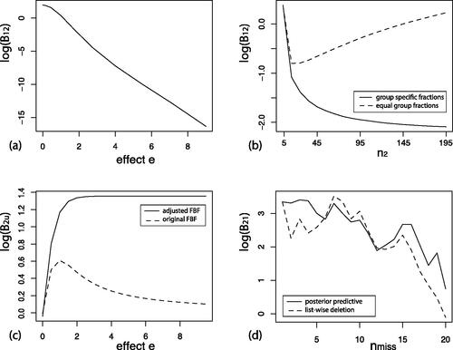
A final important difference is that the proposed adjusted fractional Bayes factor is information consistent while the Bayes factor based on the standard g prior is not information consistent (Liang et al., 2008). Information consistency implies that the evidence against an equality constrained hypothesis diverges as the observed effect goes to infinity. To obtain an information consistent Bayes factor based on the g prior, a common solution is to mix g with a prior distribution (Liang et al., 2008; Mulder et al., 2020). To see that the proposed default Bayes factor is information consistent, observe that the posterior in the numerators in (7) are centered around the OLS estimate of $\mathbf{\Theta }.$ Thus, as the evidence against an equality constraint based on the observed effects accumulates in the sense that ${\mathbf{R}}_{t,E}\widehat{\mathit{\theta }}-{\mathbf{r}}_{t,E}\to \infty ,$ then $B_{tu}^{*}$ goes to 0. To see this in our running example test of ${\mathcal{H}}_1$ against ${\mathcal{H}}_2,$ we consider data with OLS estimates of $({\widehat{\mu }}_{11},{\widehat{\mu }}_{21},{\widehat{\mu }}_{12},{\widehat{\mu }}_{22})=e(-1,0,1,2),$ while increasing e from 0 to 9, while keeping the sample sizes fixed at $N_1=N_2=5$ (the exact choice of the sample size does not qualitatively affect the result). Thus, a larger value for e implies more evidence against ${\mathcal{H}}_1$ in favor of ${\mathcal{H}}_2.$ As can be seen in Figure 1a, the evidence against ${\mathcal{H}}_1$ accumulates in accordance with the evidence based on the observed estimates while e increases.

Figure 1. (a) Illustration of information consistent behavior for the proposed Bayes factor when the observed effect e increases. (b) Illustration of the effect of different fractions across groups when the sample in group 1 is fixed at $N_1=5$ and the sample in group 2 increases. (c) Illustration of the difference between the adjusted prior mean and the unadjusted (OLS) prior mean. (d) Illustration of the change in evidence when increasing the number of random missing observations using list-wise deletion and sampling missings from the posterior predictive distribution.

Group specific fractions for unbalanced group data

A key difference between the original fractional Bayes factor and the proposed method is that different fractions are used across observations from different groups. As described in Lemma 1 a fraction of $b_i=\frac{K+P}{J{N}_j}$ is used of the i-th observation if it belongs to group j. Thus, as there are N_j observations in group j, the information of $\frac{K+P}{J}$ observations is used from group j, and as there are J groups, in total the fractional prior contains the information of K + P observations. This is exactly equal to the minimal sample size to obtain a proper posterior under the unconstrained model when using the Jefferys priors (also called minimal training sample size in the objective Bayes factor literature; see Berger and Pericchi (2004), for example).

The use of group specific fractions is important to properly control the amount of information from every group that is used to construct the fractional prior. For the running example with two groups, straightforward calculation reveals that the scale matrix in the fractional prior equals ${({\mathbf{X}}_{\mathbf{b}}^{\prime }{\mathbf{X}}_{\mathbf{b}})}^{-1}=\text{diag}(\frac{J}{K+P},\frac{J}{K+P}),$ which is independent of the sample sizes N₁ and N₂ across groups. Instead when equal fractions would be used, i.e., b_i = b, then ${({\mathbf{X}}_{\mathbf{b}}^{\prime }{\mathbf{X}}_{\mathbf{b}})}^{-1}=\text{diag}(b^{-1}{N}_1^{-1},b^{-1}{N}_2^{-1}),$ then the prior scale would be unequal for both group means in the case of unbalanced data. It has been noted in the literature that using the same fraction across different groups results in inconsistent selection behavior (De Santis & Spezzaferri, 2001; Hoijtink et al., 2019).

To see that the proposed fractional Bayes factor results in consistent behavior for unbalanced data under the multivariate normal model, we investigate the Bayes factor in our running example for a sample size of $N_1=5$ for group 1 while the sample size of group N₂ increases from $N_2=5$ to 195 when the estimates remain fixed at $({\widehat{\mu }}_{11},{\widehat{\mu }}_{21},{\widehat{\mu }}_{12},{\widehat{\mu }}_{22})=(-1,0,1,2).$ In this case we expect that the evidence for ${\mathcal{H}}_1$ against ${\mathcal{H}}_2$ decreases as the estimates are in agreement with the constraints of ${\mathcal{H}}_2$ and we increase the sample size for group 2. Figure 1b shows that this is only the case for the proposed Bayes factor with group specific fractions. When using the sample fraction on the other hand we see that the evidence for the equality hypothesis increases when the sample size for group 2 increases. This is caused by the fractional prior for group 1 which becomes more vague when the sample size of group 2 increases. This is essentially an illustration of the Bartlett-Lindley-Jeffreys paradox (Bartlett, 1957; Jeffreys, 1961; Lindley, 1957).

Prior adjustment for order-constrained testing

Due to the adjusted parameter space ${\mathbf{\Theta }}_t^{*}$ in the numerator in (5), the implied fractional prior is centered on the boundary of the constrained space because ${\mathbf{R}}_{t,E}{\mathit{\theta }}_0={\mathbf{r}}_{t,E}$ and ${\mathbf{R}}_{t,O}{\mathit{\theta }}_0={\mathbf{r}}_{t,O}$ hold, where ${\mathit{\theta }}_0$ is the vectorization of the prior location ${\mathbf{\Theta }}_0.$ As the prior probability that the order constraints hold serves as a measure of relative complexity of order-constrained parameter spaces (Klugkist et al., 2005; Mulder et al., 2010), centering the prior on the boundary results in a Bayes factor that properly incorporates the relative complexity of order-constrained hypotheses (Mulder, 2014a).

When using the original fractional Bayes factor, the fractional prior is centered around the OLS estimate, and therefore when the order constraints are supported by the data (in the sense that the OLS estimate is located in the constrained parameter space) the fractional Bayes factor may not properly balance model fit and complexity as an “Occam’s razor”. To see this in our running example we consider data where the estimates are $({\widehat{\mu }}_{11},{\widehat{\mu }}_{21},{\widehat{\mu }}_{12},{\widehat{\mu }}_{22})=e(-1,0,1,2),$ and we let e go from 0 (no effect) to 9 (in the direction of ${\mathcal{H}}_2$). Figure 1c shows the adjusted fractional Bayes factor and the original (unadjusted) fractional Bayes factor for the order hypothesis ${\mathcal{H}}_2$ against an unconstrained hypothesis where $({\widehat{\mu }}_{11},{\widehat{\mu }}_{21},{\widehat{\mu }}_{12},{\widehat{\mu }}_{22})\in {\mathbb{R}}^4$ as a function of the effect e. As the effect increases, the order hypothesis and the unconstrained hypothesis gradually receive the same amount of evidence from the data by the original fractional Bayes factor even though the constraints of the order hypothesis has a good fit and the order constrained subspace only covers a proportion of the complete unconstrained parameter space ${\mathbb{R}}^4.$ The adjusted FBF on the other hand converges to $\text{log}\hspace{0.17em}(4)$ because the posterior probability that the constraints hold goes to 1 and the prior probability remains fixed at $\frac{1}{4}$ due to the prior adjustment.

Hypothesis testing with missing observations

Missing data are ubiquitous in statistical practice. In a Bayesian framework the natural solution to missing data is to sample the data that are missing at random using the posterior predictive distribution given the observed data. Thereby, the uncertainty induced by the missing observations is properly incorporated when making inferences given the observed data (Rubin, 1987, 1996).

In hypothesis testing and model selection problems this would imply that we would need to use the posterior predictive distribution under every separate model when computing the marginal likelihoods. This can be computationally intensive when the number of models is large and when the models under investigation also contain order constraints. The advantage of the proposed method however is that direct computation of the marginal likelihoods under the models is avoided, and instead all the necessary components to compute the Bayes factors using (7) are carried out under the unconstrained model. This implies that we only need to estimate the components for all constrained hypotheses using the same posterior predictive distribution under an unconstrained model (see also Hoijtink et al., 2019). Thereby we build on the multiple imputation framework where missing observations are imputed from a posterior predictive distribution assuming a properly specified missing data model (Rubin, 1996). As such, a proper quantification of the relative evidence between the hypotheses given the observed data is only obtained when the missing observations are missing at random (MAR), assuming a well-specified model for the missing observations, possibly with additional auxiliary variables, and assuming there is enough information in the observed data.

We illustrate how this works for the posterior probability that the order constraints of ${\mathcal{H}}_2$ hold given the observed data, i.e., the numerator in the second factor in (7), when certain observations are missing at random. The computation is a direct application of the law of total probability:$$\begin{array}{c}{\text{Pr}}_u({\mu }_{11}<{\mu }_{21}, {\mu }_{12}<{\mu }_{22}|{\mathbf{Y}}_{\mathit{obs}},{\mathbf{X}}_{\mathit{obs}})=\iint {\text{Pr}}_u({\mu }_{11}<{\mu }_{21}, {\mu }_{12}<{\mu }_{22}|{\mathbf{Y}}_{\mathit{obs}},{\mathbf{X}}_{\mathit{obs}},{\mathbf{Y}}_{\mathit{miss}},{\mathbf{X}}_{\mathit{miss}})\\ p_u({\mathbf{Y}}_{\mathit{miss}},{\mathbf{X}}_{\mathit{miss}}|{\mathbf{Y}}_{\mathit{obs}},{\mathbf{X}}_{\mathit{obs}})d{\mathbf{Y}}_{\mathit{miss}}d{\mathbf{X}}_{\mathit{miss}}\\ \approx M^{-1}\sum _{m=1}^M{\text{Pr}}_u({\mu }_{11}<{\mu }_{21}, {\mu }_{12}<{\mu }_{22}|{\mathbf{Y}}_{\mathit{obs}},{\mathbf{X}}_{\mathit{obs}},{\mathbf{Y}}_{\mathit{miss}}^{(m)},{\mathbf{X}}_{\mathit{miss}}^{(m)})\end{array}$$where $p_u({\mathbf{Y}}_{\mathit{miss}},{\mathbf{X}}_{\mathit{miss}}|{\mathbf{Y}}_{\mathit{obs}},{\mathbf{X}}_{\mathit{obs}})$ denotes the posterior predictive distribution of the missings under the unconstrained model, and $({\mathbf{Y}}_{\mathit{miss}}^{(m)},{\mathbf{X}}_{\mathit{miss}}^{(m)})$ denotes the m-th draw from the posterior predictive distribution. Thus, the posterior probability based on the observed data can simply be computed as the arithmetic average of the probabilities based on the M complete data where the missings were sampled from the unconstrained posterior predictive distribution. This holds for all the four quantities in (7) for all constrained hypotheses of interest. The R package mice can easily be used for imputing random draws from the posterior predictive distribution (van Buuren, 2018; van Buuren & Groothuis-Oudshoorn, 2011).

As an illustration, we evaluate the evidence for ${\mathcal{H}}_2$ versus ${\mathcal{H}}_1$ while increasing the number of random missings in a given dataset of size $N_1=N_2=15$ and $({\widehat{\mu }}_{11},{\widehat{\mu }}_{21},{\widehat{\mu }}_{12},{\widehat{\mu }}_{22})=(-1,0,1,2).$ Over 19 steps, a random dependent variable of a random complete case was generated consecutively between the two groups. We compare the result when using list-wise deletion which is known to bias the results in estimation problems. The result is displayed in Figure 1d. As we can see using the posterior predictive distribution the evidence decreases more gradually (but still noisy due to the random selection of missings) than when using list-wise deletion. Further observe that in the last step when 19 cases have one missing observation we still see there is some evidence in the direction of ${\mathcal{H}}_2$ when using the posterior predictive distribution but the evidence is essentially zero when only using the complete cases.

Empirical applications

In this section we consider two applications of the proposed Bayesian hypothesis testing procedure. The R code can be found in Appendix D.

Order-constrained MANOVA

Silvapulle and Sen (2004) described an application where four groups of 10 male Fischer-344 rats received different dosages of vinylidene fluoride. Of each rat three serum enzymes were measured: SDH, SGOT, and SGPT. It was expected that these serum levels were affected by vinylidene fluoride. As groups 1 to 4 received increasing dosage, it is was expected that the mean serum levels increased over the groups, i.e.,$$\begin{array}{c}{\mathcal{H}}_1:{\mathit{\mu }}_1={\mathit{\mu }}_2={\mathit{\mu }}_3={\mathit{\mu }}_4\\ {\mathcal{H}}_2:{\mathit{\mu }}_1<{\mathit{\mu }}_2<{\mathit{\mu }}_3<{\mathit{\mu }}_4\\ {\mathcal{H}}_3:\text{neither}\mathrm{ }{\mathcal{H}}_1,\mathrm{ }\text{nor}\mathrm{ }{\mathcal{H}}_2,\end{array}$$where ${\mathit{\mu }}_j=({\mu }_{j1},{\mu }_{j2},{\mu }_{j3})$ denotes the serum means of SDH, SGOT, and SGPT in group j, for $j=1,\dots ,4.$ Equal prior probabilities are assumed for the three hypotheses, i.e., $P({\mathcal{H}}_1)=P({\mathcal{H}}_2)=P({\mathcal{H}}_3)=\frac{1}{3}.$ The data are part of the goric package (Gerhard & Kuiper, 2020). The descriptives of the data are given in Table 1.

Table 1. Unconstrained estimates and properties of the rats data with levels of enzyme type SDH (y₁), enzyme type SGOT (y₂), and enzyme type SGPT (y₃). Note. SDH = sorbitol dehydrogenase. SGOT = serum glutamic oxaloacetic transaminase. SGPT = serum gtutamic-pyruvic transaminase.

group	parameter			estimate ± standard error			sample size	fraction
	SDH	SGOT	SGPT	SDH	SGOT	SGPT
1	μ 11	μ12	μ13	22.7 ± 1.1	99.3 ± 5.0	61.9 ± 1.7	10	.175
2	μ21	μ22	μ23	22.8 ± 1.1	108.4 ± 5.0	63.8 ± 1.7	10	.175
3	μ31	μ32	μ33	23.7 ± 1.1	100.9 ± 5.0	60.2 ± 1.7	10	.175
4	μ41	μ42	μ43	27.3 ± 1.1	112.9 ± 5.0	52.9 ± 1.7	10	.175

To compute the Bayes factor, first the multivariate model needs to be fit using the standard lm function.

install.packages("BFpack")

install.packages("goric")

library(BFpack)

mlm1 <- lm(cbind(SDH,SGOT,SGPT) ∼ -1 + dose, data = goric::vinylidene)

The constrained hypotheses are formulated using character strings on the named parameters (where x1_on_y1 denotes the effect of named predictor variable x1 on the named outcome variable y1, different constraints within the same hypothesis are separated with a ampersand (‘&’), and hypotheses are separated with a semi-colon “;”). To see the possible named parameters on which constraints can be formulated, the function get_estimates can be used via get_estimates(mlm1).¹ For example dosed1_on_SDH is the mean of the serum enzym SDH for group with dose 1. Bayes factors and posterior probabilities can be obtained by plugging in the object mlm1 and the string with hypotheses in the BF function from BFpack:

hypothesis <- "dosed1_on_SDH = dosed2_on_ SDH = dosed3_on_SDH =

dosed4_on_SDH & dosed1_on_SGOT = dosed2_on_ SGOT = dosed3_on_SGOT =

dosed4_on_SGOT & dosed1_on_SGPT = dosed2_on_ SGPT = dosed3_on_SGPT =

dosed4_on_SGPT; dosed1_on_SDH < dosed2_on_ SDH < dosed3_on_SDH <

dosed4_on_SDH & dosed1_on_SGOT < dosed2_on_ SGOT < dosed3_on_SGOT <

dosed4_on_SGOT & dosed1_on_SGPT < dosed2_on_ SGPT < dosed3_on_SGPT <

dosed4_on_SGPT" set.seed(12) BF1 <- BF(mlm1, hypothesis) print(BF1)

round(BF1$BFtable_confirmatory,3)

Table 2 shows the four quantities $f_t^E,c_t^E,f_t^O,$ and $c_t^O$ from (7), the posterior probabilities of the three models, and the Bayes factors. By default BFpack uses equal prior probabilities, so that the posterior odds between pairs of hypotheses correspond with the respective Bayes factors. Based on these results we obtain very strong evidence for the complement hypothesis ${\mathcal{H}}_3.$ Note that eyeballing the estimates also showed no evidence in the direction of the order hypothesis. The Bayesian analysis confirms this result and provides an exact quantification of the relative of evidence in the data between the three hypotheses.

Table 2. Bayesian model selection for the rats application. In the second, third, fourth, fifth, sixth and seventh column, the relative measures of fit of the equality constraints, complexity of the equality constraints, fit of the order constraints, complexity of the order constraints, the Bayes factors against an unconstrained alternative (Equation (7)(7) $$\begin{array}{c}{B}_{tu}^{*}=\frac{f_t^E}{c_t^E}\times \frac{f_t^O}{c_t^O}\\ =\frac{{\pi }_u({\mathbf{R}}_{t,E}\mathit{\theta }={\mathbf{r}}_{t,E}|\mathbf{Y},\mathbf{X})}{{\pi }_u^{*}({\mathbf{R}}_{t,E}\mathit{\theta }={\mathbf{r}}_{t,E}|\mathbf{Y},\mathbf{X},\mathbf{b})}\times \frac{{\text{Pr}}_u({\mathbf{R}}_{t,O}\mathit{\theta }>{\mathbf{r}}_{t,O}|{\mathbf{R}}_{t,E}\mathit{\theta }={\mathbf{r}}_{t,E},\mathbf{Y},\mathbf{X})}{{\text{Pr}}_u^{*}({\mathbf{R}}_{t,O}\mathit{\theta }>{\mathbf{r}}_{t,O}|{\mathbf{R}}_{t,E}\mathit{\theta }={\mathbf{r}}_{t,E},\mathbf{Y},\mathbf{X},\mathbf{b})}\end{array}$$(7) ), and the posterior probability are presented, respectively.

Model	$f_t^E$	$c_t^E$	$f_t^O$	$c_t^O$	Btu	$B_{t1}$	$B_{t2}$	$B_{t3}$	$P({\mathcal{H}}_t|\mathbf{y})$
${\mathcal{H}}_1$	1.62e–15	1.86e–13			.009	1.000	1795.995	0.009	.009
${\mathcal{H}}_2$			1.40e–08	2.36e–3	.000	0.001	1.000	0.000	.000
${\mathcal{H}}_3$			1.000	0.998	1.002	106.057	190478.668	1.000	.991

Constrained multivariate multiple regression

Stevens (1996) presented a study concerning the effect of the first year of watching the Sesame street series on the knowledge of 240 children in the age range 34 to 69 months. To illustrate the Bayesian hypothesis test in the context of a multivariate multiple regression model, the outcome variables $y_1\mathrm{ }\text{and}\mathrm{ }{y}_2,$ which are the knowledge of body parts and the knowledge of numbers of children after watching Sesame Street, respectively, are regressed on $x_1\mathrm{ }\text{and}\mathrm{ }{x}_2,$ which are the knowledge of body parts and the knowledge of numbers of children before watching Sesame Street for a year. To facilitate replicability of this application, the data are taken from the R package bain (Gu et al., 2019; 2020). First we perform an analysis on the complete data. Second, we randomly generate 20% missing observations and perform the analysis on the list-wise deleted data, and perform the analysis using on imputed data with the posterior predictive distribution (using the mice package van Buuren & Groothuis-Oudshoorn, 2011).

The following multivariate multiple regression model will be used for $i=1,..,N,\mathrm{ }\text{where}\mathrm{ }N=240$ denotes the sample size:(10) $$\begin{array}{c}{y}_{i1}={\mu }_{11}+{\beta }_{11}{x}_{i1}+{\beta }_{21}{x}_{i2}+e_{i1}\\ y_{i2}={\mu }_{12}+{\beta }_{12}{x}_{i1}+{\beta }_{22}{x}_{i2}+e_{i2}\\ \left[\begin{array}{c}{e}_{i1}\\ e_{i2}\end{array}\right]\sim \mathcal{N}\left(\left[\begin{array}{c}0\\ 0\end{array}\right],\left[\begin{array}{cc}{\sigma }_1^2& {\sigma }_{12}\\ {\sigma }_{21}& {\sigma }_2^2\end{array}\right]\right).\end{array}$$(10)

Note that this is a cross lagged panel model with two measurement occasions. Note that, in order to ensure comparability of the regression coefficients, in this application each imputed data matrix (see below) is standardized.

The goal is to test whether the knowledge of numbers and letters before watching Sesame Street can predict the knowledge of numbers and letters after watching. Given the two different skills, it was expected that the knowledge of letters after watching Sesame Street can better be predicted by the knowledge of letters before watching Sesame Street than by the knowledge of numbers before watching Sesame Street. In the same line of reasoning, the knowledge of numbers after watching Sesame Street can better be predicted by the knowledge of numbers before watching Sesame Street than the knowledge of letters before watching Sesame Street. Furthermore, as these types of abilities are very often positively correlated, it was expected that all effects were positive. This results in the following order (or ‘informative’) hypothesis ${\mathcal{H}}_1,$ which will be tested against a traditional null hypothesis (here denoted by ${\mathcal{H}}_2$) and a complement hypothesis, denoted by ${\mathcal{H}}_3:$$$\begin{array}{c}{\mathcal{H}}_1:{\beta }_{11}>{\beta }_{21}>0 {\beta }_{22}>{\beta }_{12}>0\\ {\mathcal{H}}_2:{\beta }_{11}={\beta }_{21}=0 {\beta }_{22}={\beta }_{12}=0\\ {\mathcal{H}}_3:\mathrm{ }\text{neither}\mathrm{ }{\mathcal{H}}_1,\mathrm{ }\text{nor}\mathrm{ }{\mathcal{H}}_2.\end{array}$$

Note that it would also be possible to test constraints across dimensions (e.g., ${\beta }_{11}\mathrm{ }\text{against}\mathrm{ }{\beta }_{12}$). For illustrative purposes we limit ourselves to only testing constraints within the same dimension.

First, we perform an analysis on the complete data set. The descriptive statistics can be found in Table 3. The multivariate regression model is fit using the ‘lm’ function, and the hypotheses are formulated on the named parameters:

Table 3. Unconstrained estimates for the Sesame Street application.

parameter	estimate	standard error	correlation matrix
β11	.505	.066	1.00
β21	.188	.066	−.664 1.00
β12	.327	.062	.375 −.249 1.00
β22	.441	.062	−.249.375 −.664 1.00

library(BFpack)

# standardize data

sesamesim_st <- as.data.frame(scale(bain::sesamesim))[,c(10,13,16,19)]

# fit model

mlm2 <- lm(cbind(Ab, An) ∼ 1 + Bb + Bn, data = sesamesim_st)

# formulate hypotheses

hypothesis <-

"Bn_on_An > Bb_on_An > 0 & Bb_on_Ab > Bn_on_Ab > 0;

Bn_on_An = Bb_on_An = 0 & Bb_on_Ab = Bn_on_Ab = 0"

# perform Bayesian hypothesis test

set.seed(123)

BF2 <- BF(mlm2, hypothesis = hypothesis)

In the formulation of the hypothesis, the named parameter Bb_on_An denotes the effect of knowledge on body parts before watching Sesame Street (‘Bb’) on knowledge of numbers after watching Sesame Street (‘An’), i.e., ${\beta }_{21}.$ Table 4 shows the resulting Bayes factors and posterior probabilities, together with their building blocks in (7). The results indicate that the null hypothesis ${\mathcal{H}}_2$ can be safely ruled out. Moreover, there is approximately 700 times more evidence for the order hypothesis ${\mathcal{H}}_1$ against the complement ${\mathcal{H}}_3$ as can be seen from the Bayes factor $B_{13}=699.11.$

Table 4. Bayesian Hypothesis Evaluation for the Sesame Street application. In the second, third, fourth, fifth, sixth and seventh column, the relative measures of fit of the equality constraints, complexity of the equality constraints, fit of the order constraints, complexity of the order constraints, the Bayes factors against an unconstrained alternative (Equation (7)(7) $$\begin{array}{c}{B}_{tu}^{*}=\frac{f_t^E}{c_t^E}\times \frac{f_t^O}{c_t^O}\\ =\frac{{\pi }_u({\mathbf{R}}_{t,E}\mathit{\theta }={\mathbf{r}}_{t,E}|\mathbf{Y},\mathbf{X})}{{\pi }_u^{*}({\mathbf{R}}_{t,E}\mathit{\theta }={\mathbf{r}}_{t,E}|\mathbf{Y},\mathbf{X},\mathbf{b})}\times \frac{{\text{Pr}}_u({\mathbf{R}}_{t,O}\mathit{\theta }>{\mathbf{r}}_{t,O}|{\mathbf{R}}_{t,E}\mathit{\theta }={\mathbf{r}}_{t,E},\mathbf{Y},\mathbf{X})}{{\text{Pr}}_u^{*}({\mathbf{R}}_{t,O}\mathit{\theta }>{\mathbf{r}}_{t,O}|{\mathbf{R}}_{t,E}\mathit{\theta }={\mathbf{r}}_{t,E},\mathbf{Y},\mathbf{X},\mathbf{b})}\end{array}$$(7) ), and the posterior probability are presented, respectively.

Model	$f_t^E$	$c_t^E$	$f_t^O$	$c_t^O$	Btu	$B_{t1}$	$B_{t2}$	$B_{t3}$	$P({\mathcal{H}}_t|\mathbf{y})$
${\mathcal{H}}_1$			0.836	0.007	115.409	1.000	2.8e44	699.11	0.999
${\mathcal{H}}_2$	0.000	0.107			0.000	0.000	1.000	0.000	0.000
${\mathcal{H}}_3$			0.164	0.993	0.165	0.001	4.0e41	1.000	0.001

Next we perform an analysis after creating 20% of random missing observations in the data. The complete R code can be found in Appendix D. After list-wise deletion only have 94 complete cases left. Computing the Bayes factors for ${\mathcal{H}}_1\mathrm{ }\text{against}\mathrm{ }{\mathcal{H}}_2\mathrm{ }\text{and}\mathrm{ }{\mathcal{H}}_3\mathrm{ }\text{yields}\mathrm{ }{B}_{12}=4.6\mathrm{e}12\mathrm{ }\text{and}\mathrm{ }{B}_{13}=19.05,$ respectively. This illustrates a clear loss of the evidence in favor of the most supported hypothesis, ${\mathcal{H}}_1.$

Now we compute the Bayes factors by first estimating the four different ingredients $f_t^E,c_t^E,f_t^O,$ and $c_t^O$ using the posterior predictive distribution of the observed data (hypothesis testing with missing observations section). This was done using the mice package (van Buuren & Groothuis-Oudshoorn, 2011) (Appendix D). This results in Bayes factors of $B_{12}=1.0\mathrm{e}36\mathrm{ }\text{and}\mathrm{ }{B}_{13}=362.76.$ As can be seen, the evidence for ${\mathcal{H}}_1$ is considerably larger in comparison to the analysis after list-wise deletion. This can be explained from the fact that this analysis uses all the available information in the observed data while the analysis after list-wise deletion only uses the information from the complete cases in the data.

Discussion

A default Bayes factor was proposed for evaluating multivariate normal linear models with competing sets of equality and order constraints on the parameters of interest. The methodology has the following attractive features. First the method can be used for evaluating statistics models with equality as well as order constraints on the parameters of interest. The possibility of order constrained testing is particularly useful in the applied sciences where researchers often formulate their scientific expectations using order constraints. Second, the method is fully automatic and therefore can be applied when prior information is weak or completely unavailable. The fractional prior is based on a minimal fraction of the information in the observed data of every group so that maximal information is used for model selection. Third, the Bayes factor is relatively simple to compute via Monte Carlo estimation that can be done in parallel. The Bayes factor has analytic expressions for special cases. Fourth the criterion is consistent which implies that the true constrained model will always be selected it the sample is large enough. Fifth, in the presence of missing data that are missing at random, the Bayes factor can be computed relatively easily using a multiple imputation method only under the unconstrained model. In sum, the method gives substantive researchers a simple tool for quantifying the evidence between competing scientific expectations while also correcting for missing data that are missing at random (MAR) for many popular models including (multivariate) linear regression, (M)AN(C)OVA, repeated measures.

The methodology is implemented in the R-package BFpack (cran.r-project.org/web/packages/BFpack/index.html) which allows the applied statistical community to use the methodology in a relatively easy manner. We recommend the proposed methodology and software for default testing of multiple equality/order hypotheses when clear prior information about the magnitude of the parameters is absent or if researchers prefer to refrain from using informative priors. The hypotheses need to have been formulated before inspecting the data. Ideally, the hypotheses of interest have been preregistered to avoid possible bias on the reported evidence between the hypotheses (Hoijtink et al., 2019; Wagenmakers et al., 2012). Researchers can choose to either report the posterior probabilities of the formulated hypotheses or to report the Bayes factors between all pairs of hypotheses. Both are directly available using BFpack. One may prefer to report Bayes factors when clear prior beliefs about the hypotheses are absent.

The proposed methodology was specifically designed under the multivariate normal model which assumes normally distributed errors. Therefore a reasonable question is how robust our approach is to violations of this assumption. Answering this question falls outside of the scope of the current paper. This may be interesting for future work. We expect that the robustness of our approach is comparable to other (Bayesian and non Bayesian) approaches as the unconstrained posterior (which is the main building block for the proposed Bayes factor) becomes approximately normal for moderate to large samples (abiding large sample theory). Furthermore the robustness of Bayes factors to violations of normality reported in van Wesel et al. (2011) and Böing-Messing and Mulder (2018) was not alarming.

The proposed adjusted fractional Bayes methodology can also be extended to generalized linear models for non-normal data. This would yet be another interesting direction for future research. Until an exact Bayes factor test is available, we recommend using the approximate Bayes factor (Gu et al., 2018) as implemented in the R packages BFpack (Mulder et al., 2020) and bain (Gu et al., 2020, 2019).

As the goal of Bayesian hypothesis testing is not to control unconditional type I and type II error probabilities, but to quantify the relative evidence between hypotheses and to quantify conditional error probabilities given the observed data (via the posterior probabilities), no numerical simulations were presented to explore specificity and sensitivity. Moreover, due to the generality of the proposed method (allowing a very broad class of equality/order hypotheses under many different designs, such as (multivariate) $t$ tests, (M)AN(C)OVA, and (multivariate) regression), such simulations would only give a narrow view under very controlled settings. Further note that due to the consistency of the proposed Bayes factor, the type I and type II error probabilities will go to 0 by definition as the sample size grows. It may be interesting however to explore specificity and sensitivity under certain common designs. We leave this for future work.

In this paper the Bayes factor was used as a confirmatory tool for model selection among a specific set of models with equality and/or order constraints. Equal model prior model probabilities were considered under the assumption that all models were (approximately) equally plausible based on substantive justifications before observing the data. In a more exploratory setting other choices may be preferable, (e.g., see Scott & Berger, 2006, who considered a model selection problem of many competing equality constrained models). It will be interesting to investigate how prior model probabilities should be specified in such exploratory settings when models may contain equality as well as order constraints on the parameters of interest.

Article information

Conflict of interest disclosures: Each author signed a form for disclosure of potential conflicts of interest. No authors reported any financial or other conflicts of interest in relation to the work described.

Ethical principles: The authors affirm having followed professional ethical guidelines in preparing this work. These guidelines include obtaining informed consent from human participants, maintaining ethical treatment and respect for the rights of human or animal participants, and ensuring the privacy of participants and their data, such as ensuring that individual participants cannot be identified in reported results or from publicly available original or archival data.

Funding: The first author was supported by Grant Vidi 452-17-006 from The Netherlands Organization for Scientific Research. The second author was supported by Grant 2020PJC034 from Shanghai Pujiang Talent Program and Grant 2019ECNU-XFZH015 from the East China Normal University.

Role of the funders/sponsors: None of the funders or sponsors of this research had any role in the design and conduct of the study; collection, management, analysis, and interpretation of data; preparation, review, or approval of the manuscript; or decision to submit the manuscript for publication.

Acknowledgments: The authors would like to thank Herbert Hoijtink, two anonymous reviewers, the AE and, the editor for their comments on prior versions of this manuscript. The ideas and opinions expressed herein are those of the authors alone, and endorsement by the authors’ institutions is not intended and should not be inferred.

Notes

For more information about testing hypotheses using the R package ‘BFpack’ we refer the interested to Mulder et al. (in press).

A Derivation of the Bayes factor

The constrained hypothesis, ${\mathcal{H}}_t:{\mathbf{R}}_{t,E}\mathit{\theta }={\mathbf{r}}_{t,E} \& {\mathbf{R}}_{t,O}\mathit{\theta }>{\mathbf{r}}_{t,O}$ in (2), can equivalently be written on the transformed parameter vector$${\mathit{\zeta }}_t=\left[\begin{array}{c}{\mathit{\zeta }}_{t,E}\\ {\mathit{\zeta }}_{t,O}\\ {\mathit{\zeta }}_{t,D}\end{array}\right]=\left[\begin{array}{c}{\mathbf{R}}_{t,E}\\ {\mathbf{R}}_{t,O}\\ {\mathbf{D}}_t\end{array}\right]\mathit{\theta }={\mathbf{R}}_t\mathit{\theta },$$

so that ${\mathcal{H}}_t:{\mathit{\zeta }}_{t,E}={\mathbf{r}}_{t,E} \& {\mathit{\zeta }}_{t,O}>{\mathbf{r}}_{t,O},$ where ${\mathbf{D}}_t$ is a dummy matrix with independent rows that are permutations of $(1,0,\dots ,0),$ so that the transformation is one-to-one. In this parameterization, the (unconstrained) nuisance parameters are ${\mathit{\zeta }}_{t,D}\mathrm{ }\text{and}\mathrm{ }\mathbf{\Sigma }.$ The adjusted parameter space, ${\mathbf{\Theta }}_t^{*}=\left\{\mathit{\theta }\right|{\mathbf{R}}_{t,E}(\mathit{\theta }-\widehat{\mathit{\theta }})=\mathbf{0}, {\mathbf{R}}_{t,O}(\mathit{\theta }-\widehat{\mathit{\theta }})>\mathbf{0}\},$ then becomes ${\mathbf{Z}}_t^{*}=\left\{{\mathit{\zeta }}_t\right|{\mathit{\zeta }}_{t,E}-{\widehat{\mathit{\zeta }}}_{t,E}=\mathbf{0}, {\mathit{\zeta }}_{t,O}-{\widehat{\mathit{\zeta }}}_{t,O}>\mathbf{0}\},$ where ${\widehat{\mathit{\zeta }}}_{t,E}={\mathbf{R}}_{t,E}\widehat{\mathit{\theta }}\mathrm{ }\text{and}\mathrm{ }{\widehat{\mathit{\zeta }}}_{t,O}={\mathbf{R}}_{t,O}\widehat{\mathit{\theta }}.$

The marginal likelihood under ${\mathcal{H}}_t$ in (5) can then equivalently be written as$$p_t^{*}(\mathbf{Y},\mathbf{b})=\frac{{\int \int \int }_{{\mathit{\zeta }}_{t,O}>{\mathbf{r}}_{t,O}}p(\mathbf{Y}|\mathbf{X},{\mathit{\zeta }}_{t,E}={\mathbf{r}}_{t,E},{\mathit{\zeta }}_{t,O},{\mathit{\zeta }}_{t,D},\mathbf{\Sigma })|\mathbf{\Sigma }{|}^{-\frac{P+1}{2}}d{\mathit{\zeta }}_{t,O}d{\mathit{\zeta }}_{t,D}d\mathbf{\Sigma }}{{\int \int \int }_{{\mathit{\zeta }}_{t,O}>{\widehat{\mathit{\zeta }}}_{t,O}}p{(\mathbf{Y}|\mathbf{X},{\mathit{\zeta }}_{t,E}={\widehat{\mathit{\zeta }}}_{t,E},{\mathit{\zeta }}_{t,O},{\mathit{\zeta }}_{t,D},\mathbf{\Sigma })}^{\mathbf{b}}|\mathbf{\Sigma }{|}^{-\frac{P+1}{2}}d{\mathit{\zeta }}_{t,O}d{\mathit{\zeta }}_{t,D}d\mathbf{\Sigma }},$$

and the marginal likelihood under an unconstrained alternative, ${\mathcal{H}}_u,$ equals$$p_u(\mathbf{Y},\mathbf{b})=\frac{\int \mathrm{}\int \mathrm{}\int \mathrm{}\int p(\mathbf{Y}|\mathbf{X},{\mathit{\zeta }}_{t,E},{\mathit{\zeta }}_{t,O},{\mathit{\zeta }}_{t,D},\mathbf{\Sigma })|\mathbf{\Sigma }{|}^{-\frac{P+1}{2}}d{\mathit{\zeta }}_{t,E}d{\mathit{\zeta }}_{t,O}d{\mathit{\zeta }}_{t,D}d\mathbf{\Sigma }}{\int \mathrm{}\int \mathrm{}\int \mathrm{}\int p{(\mathbf{Y}|\mathbf{X},{\mathit{\zeta }}_{t,E},{\mathit{\zeta }}_{t,O},{\mathit{\zeta }}_{t,D},\mathbf{\Sigma })}^{\mathbf{b}}|\mathbf{\Sigma }{|}^{-\frac{P+1}{2}}d{\mathit{\zeta }}_{t,E}d{\mathit{\zeta }}_{t,O}d{\mathit{\zeta }}_{t,D}d\mathbf{\Sigma }}.$$

Thus, the Bayes factor can be written as(11) $$\begin{array}{c}{B}_{tu}=\frac{p_t^{*}(\mathbf{Y},\mathbf{b})}{p_u(\mathbf{Y},\mathbf{b})}=\frac{{\int \int \int }_{{\mathit{\zeta }}_{t,O}>{\mathbf{r}}_{t,O}}p(\mathbf{Y}|\mathbf{X},{\mathit{\zeta }}_{t,E}={\mathbf{r}}_{t,E},{\mathit{\zeta }}_{t,O},{\mathit{\zeta }}_{t,D},\mathbf{\Sigma })|\mathbf{\Sigma }{|}^{-\frac{P+1}{2}}d{\mathit{\zeta }}_{t,O}d,{\mathit{\zeta }}_{t,D}d\mathbf{\Sigma }}{{\int \int \int }_{{\mathit{\zeta }}_{t,O}>{\widehat{\mathit{\zeta }}}_{t,O}}p{(\mathbf{Y}|\mathbf{X},{\mathit{\zeta }}_{t,E}={\widehat{\mathit{\zeta }}}_{t,E},{\mathit{\zeta }}_{t,O},{\mathit{\zeta }}_{t,D},\mathbf{\Sigma })}^{\mathbf{b}}|\mathbf{\Sigma }{|}^{-\frac{P+1}{2}}d{\mathit{\zeta }}_{t,O}d,{\mathit{\zeta }}_{t,D}d\mathbf{\Sigma }}/\\ \frac{\int \mathrm{}\int \mathrm{}\int \mathrm{}\int p(\mathbf{Y}|\mathbf{X},{\mathit{\zeta }}_{t,E},{\mathit{\zeta }}_{t,O},{\mathit{\zeta }}_{t,D},\mathbf{\Sigma })|\mathbf{\Sigma }{|}^{-\frac{P+1}{2}}d{\mathit{\zeta }}_{t,E}d{\mathit{\zeta }}_{t,O}d{\mathit{\zeta }}_{t,D}d\mathbf{\Sigma }}{\int \mathrm{}\int \mathrm{}\int \mathrm{}\int p{(\mathbf{Y}|\mathbf{X},{\mathit{\zeta }}_{t,E},{\mathit{\zeta }}_{t,O},{\mathit{\zeta }}_{t,D},\mathbf{\Sigma })}^{\mathbf{b}}|\mathbf{\Sigma }{|}^{-\frac{P+1}{2}}d{\mathit{\zeta }}_{t,E}d{\mathit{\zeta }}_{t,O}d{\mathit{\zeta }}_{t,D}d\mathbf{\Sigma }}\\ ={\int \int \int }_{{\mathit{\zeta }}_{t,O}>{\mathbf{r}}_{t,O}}\frac{p(\mathbf{Y}|\mathbf{X},{\mathit{\zeta }}_{t,E}={\mathbf{r}}_{t,E},{\mathit{\zeta }}_{t,O},{\mathit{\zeta }}_{t,D},\mathbf{\Sigma })|\mathbf{\Sigma }{|}^{-\frac{P+1}{2}}}{\int \mathrm{}\int \mathrm{}\int \mathrm{}\int p(\mathbf{Y}|\mathbf{X},{\mathit{\zeta }}_{t,E},{\mathit{\zeta }}_{t,O},{\mathit{\zeta }}_{t,D},\mathbf{\Sigma })|\mathbf{\Sigma }{|}^{-\frac{P+1}{2}}d{\mathit{\zeta }}_{t,E}d{\mathit{\zeta }}_{t,O}d{\mathit{\zeta }}_{t,D}d\mathbf{\Sigma }}d{\mathit{\zeta }}_{t,O}d{\mathit{\zeta }}_{t,D}d\mathbf{\Sigma }/\\ {\int \int \int }_{{\mathit{\zeta }}_{t,O}>{\widehat{\mathit{\zeta }}}_{t,O}}\frac{p{(\mathbf{Y}|\mathbf{X},{\mathit{\zeta }}_{t,E}={\widehat{\mathit{\zeta }}}_{t,E},{\mathit{\zeta }}_{t,O},{\mathit{\zeta }}_{t,D},\mathbf{\Sigma })}^{\mathbf{b}}|\mathbf{\Sigma }{|}^{-\frac{P+1}{2}}}{\int \mathrm{}\int \mathrm{}\int \mathrm{}\int p{(\mathbf{Y}|\mathbf{X},{\mathit{\zeta }}_{t,E},{\mathit{\zeta }}_{t,O},{\mathit{\zeta }}_{t,D},\mathbf{\Sigma })}^{\mathbf{b}}|\mathbf{\Sigma }{|}^{-\frac{P+1}{2}}d{\mathit{\zeta }}_{t,E}d{\mathit{\zeta }}_{t,O}d{\mathit{\zeta }}_{t,D}d\mathbf{\Sigma }}d{\mathit{\zeta }}_{t}d\mathbf{\Sigma }\\ ={\int \int \int }_{{\mathit{\zeta }}_{t,O}>{\mathbf{r}}_{t,O}}{\pi }_u({\mathit{\zeta }}_{t,E}={\mathbf{r}}_{t,E},{\mathit{\zeta }}_{t,O},{\mathit{\zeta }}_{t,D},\mathbf{\Sigma }|\mathbf{Y},\mathbf{X})d{\mathit{\zeta }}_{t,O}d{\mathit{\zeta }}_{t,D}d\mathbf{\Sigma }/\\ {\int \int \int }_{{\mathit{\zeta }}_{t,O}>{\widehat{\mathit{\zeta }}}_{t,O}}{\pi }_u({\mathit{\zeta }}_{t,E}={\widehat{\mathit{\zeta }}}_{t,E},{\mathit{\zeta }}_{t,O},{\mathit{\zeta }}_{t,D},\mathbf{\Sigma }|\mathbf{Y},\mathbf{X},\mathbf{b})d{\mathit{\zeta }}_{t,O}d{\mathit{\zeta }}_{t,D}d\mathbf{\Sigma }\\ =\frac{{\int }_{{\mathit{\zeta }}_{t,O}>{\mathbf{r}}_{t,O}}{\pi }_u({\mathit{\zeta }}_{t,E}={\mathbf{r}}_{t,E},{\mathit{\zeta }}_{t,O}|\mathbf{Y},\mathbf{X})d{\mathit{\zeta }}_{t,O}}{{\int }_{{\mathit{\zeta }}_{t,O}>{\widehat{\mathit{\zeta }}}_{t,O}}{\pi }_u({\mathit{\zeta }}_{t,E}={\mathbf{r}}_{t,E},{\mathit{\zeta }}_{t,O}|\mathbf{Y},\mathbf{X},\mathbf{b})d{\mathit{\zeta }}_{t,O}}\\ =\frac{{\pi }_u({\mathit{\zeta }}_{t,E}={\mathbf{r}}_{t,E}|\mathbf{Y},\mathbf{X})}{{\pi }_u({\mathit{\zeta }}_{t,E}={\widehat{\mathit{\zeta }}}_{t,E}|\mathbf{Y},\mathbf{X},\mathbf{b})}\times \frac{{\text{Pr}}_u({\mathit{\zeta }}_{t,O}>{\mathbf{r}}_{t,O}|{\mathit{\zeta }}_{t,E}={\mathbf{r}}_{t,E},\mathbf{Y},\mathbf{X})}{{\text{Pr}}_u({\mathit{\zeta }}_{t,O}>{\widehat{\mathit{\zeta }}}_{t,O}|{\mathit{\zeta }}_{t,E}={\mathbf{r}}_{t,E},\mathbf{Y},\mathbf{X},\mathbf{b})}\\ =\frac{{\pi }_u({\mathit{\zeta }}_{t,E}={\mathbf{r}}_{t,E}|\mathbf{Y},\mathbf{X})}{{\pi }_u^{*}({\mathit{\zeta }}_{t,E}={\mathbf{r}}_{t,E}|\mathbf{Y},\mathbf{X},\mathbf{b})}\times \frac{{\text{Pr}}_u({\mathit{\zeta }}_{t,O}>{\mathbf{r}}_{t,O}|{\mathit{\zeta }}_{t,E}={\mathbf{r}}_{t,E},\mathbf{Y},\mathbf{X})}{{\text{Pr}}_u^{*}({\mathit{\zeta }}_{t,O}>{\mathbf{r}}_{t,O}|{\mathit{\zeta }}_{t,E}={\mathbf{r}}_{t,E},\mathbf{Y},\mathbf{X},\mathbf{b})}\\ =\frac{{\pi }_u({\mathbf{R}}_{t,E}\mathit{\theta }={\mathbf{r}}_{t,E}|\mathbf{Y},\mathbf{X})}{{\pi }_u^{*}({\mathbf{R}}_{t,E}\mathit{\theta }={\mathbf{r}}_{t,E}|\mathbf{Y},\mathbf{X},\mathbf{b})}\times \frac{{\text{Pr}}_u({\mathbf{R}}_{t,O}\mathit{\theta }>{\mathbf{r}}_{t,O}|{\mathbf{R}}_{t,E}\mathit{\theta }={\mathbf{r}}_{t,E},\mathbf{Y},\mathbf{X})}{{\text{Pr}}_u^{*}({\mathbf{R}}_{t,O}\mathit{\theta }>{\mathbf{r}}_{t,O}|{\mathbf{R}}_{t,E}\mathit{\theta },\mathbf{Y},\mathbf{X},\mathbf{b})},\end{array}$$(11)

where the adjusted default prior in the second last step is given by$${\pi }_u^{*}({\mathit{\zeta }}_{t,E},{\mathit{\zeta }}_{t,O}|\mathbf{Y},\mathbf{X},\mathbf{b})={\pi }_u({\mathit{\zeta }}_{t,E}+{\widehat{\mathit{\zeta }}}_{t,E}-{\mathbf{r}}_{t,E},{\mathit{\zeta }}_{t,O}+{\widehat{\mathit{\zeta }}}_{t,O}-{\mathbf{r}}_{t,O}|\mathbf{Y},\mathbf{X},\mathbf{b}),$$

which is centered at $({\mathbf{r}}_{t,E},{\mathbf{r}}_{t,O}),$ so that is located on the boundary of the constrained space, unlike the underlying default prior based on the original fractional Bayes factor which is centered at the ML estimates $({\widehat{\mathit{\zeta }}}_{t,E},{\widehat{\mathit{\zeta }}}_{t,O}).$

Next we derive the unconstrained marginal and conditional posteriors by applying Bayes’ theorem under ${\mathcal{H}}_u,$(12) $$\begin{array}{c}{\pi }_u(\mathit{\theta },\mathbf{\Sigma }|\mathbf{Y},\mathbf{X})\propto |\mathbf{\Sigma }{|}^{-\frac{P+1}{2}}p(\mathbf{Y}|\mathbf{X},\mathbf{\Theta },\mathbf{\Sigma })\\ \propto |\mathbf{\Sigma }{|}^{-\frac{N+P+1}{2}}\hspace{0.17em}\text{exp}\hspace{0.17em}\{-\frac{1}{2}\text{tr} {\mathbf{\Sigma }}^{-1}(\mathbf{Y}-\mathbf{X}\mathbf{\Theta })\prime (\mathbf{Y}-\mathbf{X}\mathbf{\Theta })\}\\ \propto {\pi }_u(\mathbf{\Theta }|\mathbf{Y},\mathbf{X},\mathbf{\Sigma }){\pi }_u(\mathbf{\Sigma }|\mathbf{Y},\mathbf{X}),\\ \text{with}\mathrm{ }\pi (\mathbf{\Theta }|\mathbf{Y},\mathbf{X},\mathbf{\Sigma })={\mathcal{N}}_{K,P}(\widehat{\mathbf{\Theta }},{(\mathbf{X}\prime \mathbf{X})}^{-1},\mathbf{\Sigma })\end{array}$$(12) (13) $$\pi (\mathbf{\Sigma }|\mathbf{Y},\mathbf{X})=\mathcal{I}\mathcal{W}(N-K,\mathbf{S})$$(13)

where the least squares estimate is given by $\widehat{\mathbf{\Theta }}={(\mathbf{X}\prime \mathbf{X})}^{-1}\mathbf{X}\prime \mathbf{Y}$ and the sums of square matrix equals $\mathbf{S}=(\mathbf{Y}-\mathbf{X}\widehat{\mathbf{\Theta }})\prime (\mathbf{Y}-\mathbf{X}\widehat{\mathbf{\Theta }}).$ Furthermore, ${\mathcal{N}}_{K,P}\mathrm{ }\text{and}\mathrm{ }\mathcal{I}\mathcal{W}$ denote a matrix normal distribution for a $K\times P$ matrix and an inverse Wishart distribution, respectively. Note that the conditional posterior distribution for $\mathbf{\Theta }$ is equivalent to a multivariate normal on the vectorization, $\pi (\mathit{\theta }|\mathbf{Y},\mathbf{X},\mathbf{\Sigma })=\mathcal{N}(\widehat{\mathit{\theta }},\mathbf{\Sigma }\otimes {(\mathbf{X}\prime \mathbf{X})}^{-1}).$ Integrating the covariance matrix out results in a marginal posterior for $\mathbf{\Theta }$ having a $K\times P$ matrix Student $t$ distribution,$$\pi (\mathbf{\Theta }|\mathbf{Y},\mathbf{X})={\mathcal{T}}_{K,P}(\widehat{\mathbf{\Theta }},{(\mathbf{X}\prime \mathbf{X})}^{-1},\mathbf{S},N-K-P+1).$$

The unconstrained fractional prior is obtained by first raising the likelihood of the $i$-th observation to a fraction $b_i,$ i.e.,$$\begin{array}{c}p{({\mathbf{y}}_i|{\tilde{\mathbf{x}}}_i,\mathbf{\Theta },\mathbf{\Sigma })}^{b_i}\propto |\mathbf{\Sigma }{|}^{-\frac{b_i}{2}}\hspace{0.17em}\text{exp}\hspace{0.17em}\{-\frac{b_i}{2}({\mathbf{y}}_i-\mathbf{\Theta }\prime {\tilde{\mathbf{x}}}_i)\prime {\mathbf{\Sigma }}^{-1}({\mathbf{y}}_i-\mathbf{\Theta }\prime {\tilde{\mathbf{x}}}_i)\}\\ =|\mathbf{\Sigma }{|}^{-\frac{b_i}{2}}\hspace{0.17em}\text{exp}\hspace{0.17em}\{-\frac{1}{2}({\mathbf{y}}_{i,b_i}-\mathbf{\Theta }\prime {\tilde{\mathbf{x}}}_{i,b_i})\prime {\mathbf{\Sigma }}^{-1}({\mathbf{y}}_{i,b_i}-\mathbf{\Theta }\prime {\tilde{\mathbf{x}}}_{i,b_i})\},\end{array}$$

where ${\mathbf{y}}_{i,b_i}=\sqrt{b_i}{\mathbf{y}}_i\mathrm{ }\text{and}\mathrm{ }{\tilde{\mathbf{x}}}_{i,b_i}=\sqrt{b_i}{\tilde{\mathbf{x}}}_i,$ with ${\tilde{\mathbf{x}}}_i^{\prime }=({\mathbf{d}}_i,{\mathbf{x}}_i^{\prime }).$ The likelihood raised to observation specific fractions is then defined as$$\begin{array}{c}p{(\mathbf{Y}|\mathbf{X},\mathbf{\Theta },\mathbf{\Sigma })}^{\mathbf{b}}\equiv \prod _{i=1}^{n}p{({\mathbf{y}}_i|{\tilde{\mathbf{x}}}_i,\mathbf{\Theta },\mathbf{\Sigma })}^{b_i}\\ \propto |\mathbf{\Sigma }{|}^{-\frac{1}{2}\sum _{i=1}^n{b}_i}\hspace{0.17em}\text{exp}\hspace{0.17em}\{-\frac{1}{2}\text{tr} {\mathbf{\Sigma }}^{-1}({\mathbf{Y}}_{\mathbf{b}}-{\mathbf{X}}_{\mathbf{b}}\mathbf{\Theta })\prime ({\mathbf{Y}}_{\mathbf{b}}-{\mathbf{X}}_{\mathbf{b}}\mathbf{\Theta })\}\\ =|\mathbf{\Sigma }{|}^{-\frac{1}{2}\sum _{i=1}^n{b}_i}\hspace{0.17em}\text{exp}\hspace{0.17em}\{-\frac{1}{2}\text{tr} {\mathbf{\Sigma }}^{-1}{\mathbf{S}}_{\mathbf{b}}\}\\ \hspace{0.17em}\text{exp}\hspace{0.17em}\{-\frac{1}{2}\text{tr} {\mathbf{\Sigma }}^{-1}(\mathbf{\Theta }-{\widehat{\mathbf{\Theta }}}_{\mathbf{b}})\prime \mathbf{X}{\prime }_{\mathbf{b}}{\mathbf{X}}_{\mathbf{b}}(\mathbf{\Theta }-{\widehat{\mathbf{\Theta }}}_{\mathbf{b}})\},\end{array}$$

where the least squares estimate is given by ${\widehat{\mathbf{\Theta }}}_{\mathbf{b}}={(\mathbf{X}{\prime }_{\mathbf{b}}{\mathbf{X}}_{\mathbf{b}})}^{-1}{\mathbf{X}}_{\mathbf{b}}^{\prime }{\mathbf{Y}}_{\mathbf{b}}$ and the sums of square matrix equals ${\mathbf{S}}_{\mathbf{b}}=({\mathbf{Y}}_{\mathbf{b}}-{\mathbf{X}}_{\mathbf{b}}{\widehat{\mathbf{\Theta }}}_{\mathbf{b}})\prime ({\mathbf{Y}}_{\mathbf{b}}-{\mathbf{X}}_{\mathbf{b}}{\widehat{\mathbf{\Theta }}}_{\mathbf{b}}),$ and ${\mathbf{Y}}_{\mathbf{b}}\mathrm{ }\text{and}\mathrm{ }{\mathbf{X}}_{\mathbf{b}}$ are the stacked matrices of ${\mathbf{y}}_{i,b_i}\prime \mathrm{ }\text{and}\mathrm{ }{\tilde{\mathbf{x}}}_{i,b_i}\prime ,$ respectively. In combination with the improper noninformative independence Jeffreys’ prior, the fractional prior based on generalized fractional Bayes methodology can then be written as$$\begin{array}{c}{\pi }_u(\mathbf{\Theta },\mathbf{\Sigma }|\mathbf{Y},\mathbf{X},\mathbf{b})\propto |\mathbf{\Sigma }{|}^{-\frac{P+1}{2}}p{(\mathbf{Y}|\mathbf{X},\mathbf{\Theta },\mathbf{\Sigma })}^{\mathbf{b}}\\ \propto \pi (\mathbf{\Theta }|\mathbf{\Sigma },\mathbf{Y},\mathbf{X},\mathbf{b}){\pi }_u(\mathbf{\Sigma }|\mathbf{Y},\mathbf{X},\mathbf{b}),\\ \text{with}\mathrm{ }{\pi }_u(\mathbf{\Theta }|\mathbf{\Sigma },\mathbf{Y},\mathbf{X},\mathbf{b})={\mathcal{N}}_{K,P}({\widehat{\mathbf{\Theta }}}_{\mathbf{b}},{(\mathbf{X}{\prime }_{\mathbf{b}}{\mathbf{X}}_{\mathbf{b}})}^{-1},\mathbf{\Sigma }),\\ {\pi }_u(\mathbf{\Sigma }|\mathbf{Y},\mathbf{X},\mathbf{b})=\mathcal{I}\mathcal{W}(\sum _{i=1}^n{b}_i-K,{\mathbf{S}}_{\mathbf{b}}),\end{array}$$

so that$${\pi }_u(\mathbf{\Theta }|\mathbf{Y},\mathbf{X},\mathbf{b})={\mathcal{T}}_{K,P}({\widehat{\mathbf{\Theta }}}_{\mathbf{b}},{\mathbf{S}}_{\mathbf{b}},{(\mathbf{X}{\prime }_{\mathbf{b}}{\mathbf{X}}_{\mathbf{b}})}^{-1},\sum _{i=1}^N{b}_i-K-P+1).$$

The adjusted fractional prior is obtained by shifting the fractional prior to the location ${\mathbf{\Theta }}_0,$ such that ${\mathbf{R}}_{t,E}{\mathit{\theta }}_0={\mathbf{r}}_{t,E}\mathrm{ }\text{and}\mathrm{ }{\mathbf{R}}_{t,O}{\mathit{\theta }}_0={\mathbf{r}}_{t,O}$ holds, i.e., ${\mathit{\theta }}_0=[{\mathbf{R}}_{t,E}^{-1} {\mathbf{R}}_{t,O}^{-1}][{\mathbf{r}}_{t,E}^{\prime } \mathbf{r}{\prime }_{t,O}]\prime ,$ where we use the generalized Moore-Penrose matrix inverse. This yields$$\begin{array}{c}{\pi }_u^{*}(\mathbf{\Theta }|\mathbf{Y},\mathbf{X},\mathbf{b})={\pi }_u(\mathbf{\Theta }+{\widehat{\mathbf{\Theta }}}_{\mathbf{b}}-{\mathbf{\Theta }}_0|\mathbf{Y},\mathbf{X},\mathbf{b})\\ ={\mathcal{T}}_{K,P}({\mathbf{\Theta }}_0,{\mathbf{S}}_{\mathbf{b}},{(\mathbf{X}{\prime }_{\mathbf{b}}{\mathbf{X}}_{\mathbf{b}})}^{-1},\sum _{i=1}^N{b}_i-K-P+1),\end{array}$$

which is equivalent to$$\begin{array}{c}{\pi }_u^{*}(\mathbf{\Theta }|\mathbf{\Sigma },\mathbf{Y},\mathbf{X},\mathbf{b})={\mathcal{N}}_{K,P}({\mathbf{\Theta }}_0,{(\mathbf{X}{\prime }_{\mathbf{b}}{\mathbf{X}}_{\mathbf{b}})}^{-1},\mathbf{\Sigma })\\ {\pi }_u^{*}(\mathbf{\Sigma }|\mathbf{Y},\mathbf{X},\mathbf{b})=\mathcal{I}\mathcal{W}(\sum _{i=1}^N{b}_i-K,{\mathbf{S}}_{\mathbf{b}}).\end{array}$$

B Bayes factor computation

B.1 General case

If the marginal posterior for the parameter matrix $\mathbf{\Theta }$ has a matrix-variate Student $t$ distribution, the marginal posterior of the vectorization $\mathit{\theta }=\text{vec}(\mathbf{\Theta })$ does not follow a multivariate Student $t$ distribution; only the marginal distributions of the separate columns or rows of $\mathbf{\Theta }$ have multivariate $t$ distributions (Box & Tiao, 1973, p. 443). Consequently, a linear combination of the elements in $\mathit{\theta },$ say, ${\mathit{\zeta }}_{t,E}={\mathbf{R}}_{t,E}\mathit{\theta },$ does not have a multivariate student $t$ distribution or other known distributional form for a coefficient matrix ${\mathbf{R}}_{t,E}$ in general. Therefore, the posterior density in the numerator in the first term in (7) does not have an analytic form. A Monte Carlo estimate can be obtained relatively easy however. First we define the one-to-one transformation as in Appendix A, i.e., ${\mathit{\zeta }}_t=({\mathit{\zeta }}_{t,E}^{\prime },{\mathit{\zeta }}_{t,O}^{\prime },{\mathit{\zeta }}_{t,D}^{\prime })\prime =\left[{\mathbf{R}}_{t,E}^{\prime },{\mathbf{R}}_{t,O}^{\prime },{\mathbf{D}}_t^{\prime }\right]\mathit{\theta }={\mathbf{R}}_t\mathit{\theta }.$ Conditionally on $\mathbf{\Sigma },$ the transformed parameters, ${\mathit{\zeta }}_t,$ have a multivariate normal conditional posterior, $\mathcal{N}({\mathit{\mu }}_{{\mathit{\zeta }}_t},{\mathbf{\Psi }}_{{\mathit{\zeta }}_t}),$ with ${\mathit{\mu }}_{{\mathit{\zeta }}_t}={\mathbf{R}}_t\widehat{\mathit{\theta }}\mathrm{ }\text{and}\mathrm{ }{\mathbf{\Psi }}_{{\mathit{\zeta }}_t}={\mathbf{R}}_t[\mathbf{\Sigma }\otimes {(\mathbf{X}\prime \mathbf{X})}^{-1}]{\mathbf{R}}_t^{\prime }.$ Then,(14) $$\begin{array}{c}{\pi }_u({\mathbf{R}}_{t,E}\mathit{\theta }={\mathbf{r}}_{t,E}|\mathbf{Y},\mathbf{X})=\iint {\pi }_u({\mathit{\zeta }}_{t,E}={\mathbf{r}}_{t,E},{\mathit{\zeta }}_{t,O},{\mathit{\zeta }}_{t,D}|\mathbf{Y},\mathbf{X})d{\mathit{\zeta }}_{t,O}d{\mathit{\zeta }}_{t,D}\\ =\int \int \int {\pi }_u({\mathit{\zeta }}_{t,E}={\mathbf{r}}_{t,E},{\mathit{\zeta }}_{t,O},{\mathit{\zeta }}_{t,D}|\mathbf{Y},\mathbf{X},\mathbf{\Sigma }){\pi }_u(\mathbf{\Sigma }|\mathbf{Y},\mathbf{X})d\mathbf{\Sigma }d{\mathit{\zeta }}_{t,O}d{\mathit{\zeta }}_{t,D}\\ \approx S^{-1}\sum _{s=1}^S{\mathcal{N}}_{r_{t,E}}({\mathbf{r}}_{t,E};{\mathbf{R}}_{t,E}\widehat{\mathit{\theta }},{\mathbf{R}}_{t,E}[{\mathbf{\Sigma }}^{(s)}\otimes {(\mathbf{X}\prime \mathbf{X})}^{-1}]{\mathbf{R}}_{t,E}^{\prime }),\end{array}$$(14)

where ${\mathbf{\Sigma }}^{(s)}\sim \mathcal{I}\mathcal{W}(N-K,\mathbf{S}),$ for $s=1,\dots ,S,$ and ${\mathcal{N}}_{r_{t,E}}(\mathbf{r};\mathit{\mu },\mathbf{\Psi })$ denotes a $r_{t,E}$-variate normal density with mean vector $\mathit{\mu }$ and covariance matrix $\mathbf{\Psi }$ evaluated at $\mathbf{r},$ which has an analytic expression (in R, for instance, it can be computed using the dmvnorm function from the mvtnorm package). This Monte Carlo estimate can be obtained via parallelized computation, and it is therefore computationally cheap.

The conditional posterior probability in the numerator in the second term can be obtained in a similar manner. First note that the order constraints ${\mathbf{R}}_{t,O}\mathit{\theta }>{\mathbf{r}}_{t,O}$ for the transformed parameter vector are equivalent to ${\mathit{\zeta }}_{t,O}>{\mathbf{r}}_{t,O}.$ Furthermore, a property of the multivariate normal distribution is that the conditional posterior of $({\mathit{\zeta }}_{t,O},{\mathit{\zeta }}_{t,D})\mathrm{ }\text{given}\mathrm{ }{\mathit{\zeta }}_{t,E}={\mathbf{r}}_{t,E}$ has a multivariate normal distribution, and the respective marginal (conditional) posterior of ${\mathit{\zeta }}_{t,O}$ also has a multivariate normal distribution where we denote the mean and covariance matrix by ${\mathit{\mu }}_{{\mathit{\zeta }}_t,O|E}\mathrm{ }\text{and}\mathrm{ }{\mathbf{\Psi }}_{{\mathit{\zeta }}_t,O|E},$ respectively.$$\begin{array}{c}{\text{Pr}}_u({\mathbf{R}}_{t,O}\mathit{\theta }>{\mathbf{r}}_{t,O}|{\mathbf{R}}_{t,E}\mathit{\theta }={\mathbf{r}}_{t,E},\mathbf{Y},\mathbf{X})={\text{Pr}}_u({\mathit{\zeta }}_{t,O}>{\mathbf{r}}_{t,O}|{\mathit{\zeta }}_{t,E}={\mathbf{r}}_{t,E},\mathbf{Y},\mathbf{X})\\ \approx S^{-1}\sum _{s=1}^S{\Phi }_{\mathcal{N}}(-{\mathbf{r}}_{t,O};-{\mathit{\mu }}_{{\mathit{\zeta }}_t,O|E},{\mathbf{\Psi }}_{{\mathit{\zeta }}_t,O|E}^{(s)}),\end{array}$$

where ${\mathbf{\Psi }}_{{\mathit{\zeta }}_t,O|E}^{(s)}$ is computed using the $s$-th posterior draw of the error covariance matrix, ${\mathbf{\Sigma }}^{(s)}\sim \mathcal{I}\mathcal{W}(N-K,\mathbf{S}),$ for $s=1,\dots ,S,$ and ${\Phi }_{\mathcal{N}}$ denotes the multivariate normal cdf. Note that the cdf can be computed using standard statistical software (e.g., using the pmvnorm function from the mvtnorm package in R).

Note that if the sample size is sufficiently large, the matrix $t$ can be well approximated using a matrix normal distribution, ${\mathcal{N}}_{K\times P}(\widehat{\mathbf{\Theta }},{(\mathbf{X}\prime \mathbf{X})}^{-1},{(N-K-P+1)}^{-1}\mathbf{S})$ (Box & Tiao, 1973, p. 447). In this case no Monte Carlo estimate would be needed as the posterior density and the posterior probability could directly be computed using the approximated matrix (or multivariate) normal distribution of $\mathbf{\Theta }$ (or $\mathit{\theta }$).

B.2 Special cases with analytic expressions

The marginal distribution of a column (or row) of a matrix random variable with a matrix Student $t$ distribution has a multivariate Student $t$ distribution (Box & Tiao, 1973, p. 442-443). This implies that the unconstrained marginal prior and posterior of the $p$-th column of $\mathbf{\Theta },$ denoted by ${\mathit{\theta }}_p,$ are distributed as$$\begin{array}{c}{\pi }_u({\mathit{\theta }}_p|\mathbf{Y},\mathbf{X})={\mathcal{T}}_K({\widehat{\mathit{\theta }}}_p,{(N-K-P+1)}^{-1}{s}_{pp}{(\mathbf{X}\prime \mathbf{X})}^{-1},N-K-P+1)\\ {\pi }_u^{*}({\mathit{\theta }}_p|\mathbf{Y},\mathbf{X},\mathbf{b})={\mathcal{C}}_K({\mathit{\theta }}_{0,p},s_{\mathbf{b},pp}{(\mathbf{X}{\prime }_{\mathbf{b}}{\mathbf{X}}_{\mathbf{b}})}^{-1}),\end{array}$$

where $s_{\mathbf{b},pp}\mathrm{ }\text{and}\mathrm{ }{s}_{pp}$ denote the $(p,p)$-th element of ${\mathbf{S}}_{\mathbf{b}}\mathrm{ }\text{and}\mathrm{ }\mathbf{S},$ respectively. Thus, using standard calculus, it can be shown that for a constrained model with only constraints on the elements in column $p,$ i.e., ${\mathcal{H}}_t:{\mathbf{R}}_{t,E}{\mathit{\theta }}_p={\mathbf{r}}_{t,E} \& {\mathbf{R}}_{t,O}{\mathit{\theta }}_p>{\mathbf{r}}_{t,O},$ the posterior and prior quantities in (7) are equal to$$\begin{array}{c}{f}_t^E(\mathbf{Y},\mathbf{X})=\mathcal{T}({\mathbf{r}}_{t,E};{\mathbf{R}}_{t,E}{\widehat{\mathit{\theta }}}_p,{(N-K-P+1)}^{-1}{s}_{pp}{\mathbf{R}}_{t,E}{(\mathbf{X}\prime \mathbf{X})}^{-1}{\mathbf{R}}_{t,E}^{\prime },\\ N-K-P+1)\\ c_t^E(\mathbf{Y},\mathbf{X},\mathbf{b})=\mathcal{C}({\mathbf{r}}_{t,E};{\mathbf{R}}_{t,E}{\mathit{\theta }}_{0,p},s_{\mathbf{b},pp}{\mathbf{R}}_{t,E}{(\mathbf{X}{\prime }_{\mathbf{b}}{\mathbf{X}}_{\mathbf{b}})}^{-1}{\mathbf{R}}_{t,E}^{\prime })\\ f_t^O(\mathbf{Y},\mathbf{X})={\Psi }_{\mathcal{T}}(-{\mathbf{r}}_{t,O};-{\mathit{\mu }}_{{\mathit{\eta }}_t,O}^f,{\mathbf{\Psi }}_{{\mathit{\eta }}_t,O}^f,N-K-P+1)\\ c_t^O(\mathbf{Y},\mathbf{X},\mathbf{b})={\Psi }_{\mathcal{C}}(\mathbf{0};\mathbf{0},{\mathbf{\Psi }}_{{\mathit{\eta }}_t,O}^c)\end{array}$$

where ${\Psi }_{\mathcal{T}}(\mathbf{x};\mathit{\mu },\mathbf{\Psi },\nu )$ is the cdf of a multivariate Student $t$ distribution at $\mathbf{x}$ with location $\mathit{\mu },$ scale matrix $\mathbf{\Psi },$ and $\nu$ degrees of freedom, ${\Psi }_{\mathcal{C}}(\mathbf{x};\mathit{\mu },\mathbf{\Psi })$ is the cdf of a multivariate Cauchy distribution at $\mathbf{x}$ with location $\mathit{\mu }$ and scale matrix $\mathbf{\Psi },$ and$$\begin{array}{c}{\mathit{\mu }}_{{\mathit{\eta }}_t,O}^f={\mathbf{R}}_{t,O}{\widehat{\mathit{\theta }}}_p+{\mathbf{R}}_{t,O}{(\mathbf{X}\prime \mathbf{X})}^{-1}{\mathbf{R}}_{t,E}^{\prime }{({\mathbf{R}}_{t,E}{(\mathbf{X}\prime \mathbf{X})}^{-1}{\mathbf{R}}_{t,E}^{\prime })}^{-1}({\mathbf{r}}_{t,E}-{\mathbf{R}}_{t,E}{\widehat{\mathit{\theta }}}_p)\\ {\mathbf{\Psi }}_{{\mathit{\eta }}_t,O}^f=\frac{s_{pp}+({\mathbf{r}}_{t,E}-{\mathbf{R}}_{t,E}{\widehat{\mathit{\theta }}}_p)\prime {({\mathbf{R}}_{t,E}{(\mathbf{X}\prime \mathbf{X})}^{-1}{\mathbf{R}}_{t,E}^{\prime })}^{-1}({\mathbf{r}}_{t,E}-{\mathbf{R}}_{t,E}{\widehat{\mathit{\theta }}}_p)}{N-K-P+1+r_{t,E}}\\ {\mathbf{R}}_{t,O}{(\mathbf{X}\prime \mathbf{X})}^{-1}\left({\mathbf{I}}_{K-r_{t,E}}-{\mathbf{R}}_{t,E}^{\prime }{({\mathbf{R}}_{t,E}{(\mathbf{X}\prime \mathbf{X})}^{-1}{\mathbf{R}}_{t,E}^{\prime })}^{-1}{\mathbf{R}}_{t,E}{(\mathbf{X}\prime \mathbf{X})}^{-1}\right){\mathbf{R}}_{t,O}^{\prime }\\ {\mathbf{\Psi }}_{{\mathit{\eta }}_t,O}^c=\frac{s_{\mathbf{b},pp}}{1+r_{t,E}}{\mathbf{R}}_{t,O}{(\mathbf{X}{\prime }_{\mathbf{b}}{\mathbf{X}}_{\mathbf{b}})}^{-1}({\mathbf{I}}_{K-r_{t,E}}-{(\mathbf{X}{\prime }_{\mathbf{b}}{\mathbf{X}}_{\mathbf{b}})}^{-1}{\mathbf{R}}_{t,E}^{\prime }{({\mathbf{R}}_{t,E}{(\mathbf{X}{\prime }_{\mathbf{b}}{\mathbf{X}}_{\mathbf{b}})}^{-1}{\mathbf{R}}_{t,E}^{\prime })}^{-1}\\ {\mathbf{R}}_{t,E}{({\mathbf{X}}_{\mathbf{b}}^{\prime }{\mathbf{X}}_{\mathbf{b}})}^{-1}){\mathbf{R}}_{t,O}^{\prime },\end{array}$$

where $r_{t,E}$ is the number of rows of ${\mathbf{R}}_{t,E}.$ Note that the cdf’s can be computed using standard functions in statistical software (e.g., using pmvt in the mvtnorm-package (Genz et al., 2016))

Hence, the proposed default Bayes factor has an analytic expression for univariate testing problems (e.g., AN(C)OVA or linear regression), for multivariate/univariate $t$ tests, or in other testing problems where the constraints are formulated solely on the elements of one specific column or row of $\mathbf{\Theta }.$

C Sketch of the proof for consistency

First note that the unconstrained posterior density in the numerator in the first term in (7) goes to infinity if the equality constraints hold, and to zero if they do not hold. Second, the conditional posterior probability in the numerator in the second term goes to 1 if the constraints hold and to 0 if they do not hold. The quantities in the denominators depend on the unconstrained matrix-variate Cauchy prior with scale matrices ${(\mathbf{X}{\prime }_{\mathbf{b}}{\mathbf{X}}_{\mathbf{b}})}^{-1}\mathrm{ }\text{and}\mathrm{ }{\mathbf{S}}_{\mathbf{b}}.$ As the sample sizes, $n_j$ for all groups go to infinity, these scale matrices converge to finite scale matrices which depend on the population distributions of the observed variables. Note that $\mathbf{X}{\prime }_{\mathbf{b}}{\mathbf{X}}_{\mathbf{b}}=\frac{P+K}{J}{\sum }_{j=1}^J{N}_j^{-1}{\mathbf{X}}_j^{\prime }{\mathbf{X}}_j,$ where ${\mathbf{X}}_j$ is the design matrix based on group $j.$ Here, ${\sum }_{j=1}^J{N}_j^{-1}{\mathbf{X}}_j^{\prime }{\mathbf{X}}_j$ converges to$$\left[\begin{array}{cccc}1& 0& 0& E\left\{\mathbf{x}{\prime }_1\right\}\\ 0& \ddots & 0& ⋮\\ 0& 0& 1& E\left\{\mathbf{x}{\prime }_J\right\}\\ E\left\{{\mathbf{x}}_1\right\}& \cdots & E\left\{{\mathbf{x}}_J\right\}& \sum _{j}E\left\{{\mathbf{x}}_j{\mathbf{x}}_j^{\prime }\right\}\end{array}\right],$$

as $N_j\to \infty$ with the same rate, for all $j=1,\dots ,J.$ Similar results hold for the matrices ${\sum }_{j=1}^J{N}_j^{-1}{\mathbf{X}}_j^{\prime }{\mathbf{Y}}_j\mathrm{ }\text{and}\mathrm{ }{\sum }_{j=1}^J{N}_j^{-1}{\mathbf{Y}}_j^{\prime }{\mathbf{Y}}_j$ in$$\begin{array}{c}{\mathbf{S}}_{\mathbf{b}}=\mathbf{Y}{\prime }_{\mathbf{b}}{\mathbf{Y}}_{\mathbf{b}}-\mathbf{Y}{\prime }_{\mathbf{b}}{\mathbf{X}}_{\mathbf{b}}{(\mathbf{X}{\prime }_{\mathbf{b}}{\mathbf{X}}_{\mathbf{b}})}^{-1}\mathbf{X}{\prime }_{\mathbf{b}}{\mathbf{Y}}_{\mathbf{b}}\\ =\frac{P+K}{J}\left(\sum _{j=1}^J{N}_j^{-1}{\mathbf{X}}_j^{\prime }{\mathbf{Y}}_j-(\sum _{j=1}^J{N}_j^{-1}{\mathbf{Y}}_j^{\prime }{\mathbf{X}}_j){(\sum _{j=1}^J{N}_j^{-1}{\mathbf{X}}_j^{\prime }{\mathbf{X}}_j)}^{-1}(\sum _{j=1}^J{N}_j^{-1}{\mathbf{X}}_j^{\prime }{\mathbf{Y}}_j)\right)\end{array}$$

in the limit. The unconstrained default prior distribution therefore converges to some fixed matrix Cauchy distribution. This implies that the value of the prior density in the denominator in the first term in (7) converges to some positive constant as well as the conditional prior probability in the numerator in the second term for all constrained models under consideration. Consequently the Bayes factor $B_{tu}$ for a true constrained model $M_t$ goes to infinity, and $B_{tu}$ converges to zero for an incorrect model. The proposed default Bayes factor is therefore consistent.

D R code for second empirical application with missing data

set.seed(123) #create 20 missings missings <-.2 n <- nrow(sesamesim_st)

#create data frame with incomplete observations

sesamesim_st_incomplete <- sesamesim_st # create random missings

for(r in 1:nrow(sesamesim_st_incomplete)) { miss_row <- runif(4)<missings sesamesim_st_incomplete[r,miss_row] <- NA }

# Perform Bayesian hypothesis test after list-wise deletion

sesamesim_st_LD <- sesamesim_st_incomplete[!is.na(

apply(sesamesim_st_incomplete,1,sum)),] mlm2_LD <- lm(cbind(An,Ab) ∼

1 + Bn + Bb, data = sesamesim_st_LD) BF2_LD <-

BF(mlm2_LD,hypothesis = hypothesis) summary(BF2_LD) # Perform Bayesian

hypothesis test using the posterior predictive # distribution using

MICE package library(mice) # create 100 imputed data sets M <- 100

sesamesim_st_mice <- mice(data = sesamesim_ st_incomplete, m = M,

seed = 999, meth = c("norm","norm","norm","norm"), diagnostics = FALSE,

printFlag = FALSE) BFtable_complete <- lapply(1:M,function(m){

mlm2_MI <- lm(cbind(An,Ab) ∼ 1 + Bn + Bb, data = complete(sesamesim_st_mice, m)) BF2_MI <- BF(mlm2_MI, hypothesis

= hypothesis) return(BF2_MI$BFtable_confirmatory) }) comp_E <-apply(matrix(unlist(lapply(1:M, function(m){

BFtable_complete[[m]][,1]})), ncol = M),1,mean) comp_O <-apply(matrix(unlist(lapply(1:M,function(m){

BFtable_complete[[m]][,2] })), ncol = M),1,mean) fit_E <-apply(matrix(unlist(lapply(1:M, function(m){

BFtable_complete[[m]][,3]})), ncol = M),1,mean) fit_O <-apply(matrix(unlist(lapply(1:M,function(m){

BFtable_complete[[m]][,4] })),ncol = M),1,mean) BFmatrix <-matrix(c(fit_E, comp_E,fit_O, comp_O), ncol = 4) BFmatrix <-cbind(BFmatrix, fit_O*fit_E/(comp_O*comp_E)) BFmatrix <-cbind(BFmatrix,BFmatrix[,5]/sum(BFmatrix[,5])) row.names(BFmatrix) <- c("H1","H2","H3") colnames(BFmatrix) <-c("f_E","c_E","f_O","c_O","BF","PMP") # Bayes factors of H1 against

H1, H2, and H3 BFmatrix[1,5]/BFmatrix[,5]

References

- Bartlett, M. (1957). A comment on D. V. Lindley’s statistical paradox. Biometrika, 44(3–4), 533–534. https://doi.org/10.1093/biomet/44.3-4.533
- Berger, J. O., & Mortera, J. (1995). Discussion to fractional bayes factors for model comparison (by O’Hagan). Journal of the Royal Statistical Society Series B, 56, 130.
- Berger, J. O., & Pericchi, L. R. (1996). The intrinsic Bayes factor for model selection and prediction. Journal of the American Statistical Association, 91(433), 109–122. Retrieved from https://doi.org/10.1080/01621459.1996.10476668
- Berger, J. O., & Pericchi, L. R. (2004). Training samples in objective Bayesian model selection. The Annals of Statistics, 32(3), 841–869. Retrieved from https://doi.org/10.1214/009053604000000229
- Böing-Messing, F., & Mulder, J. (2018). Automatic bayes factors for testing equality- and inequality-constrained hypotheses on variances. Psychometrika, 83(3), 586–617. Retrieved from 10.1007/s11336-018-9615-z https://doi.org/10.1007/s11336-018-9615-z
- Böing-Messing, F., van Assen, M. A. L. M., Hofman, A. D., Hoijtink, H., & Mulder, J. (2017). Bayesian evaluation of constrained hypotheses on variances of multiple independent groups. Psychological Methods, 22(2), 262–287. Retrieved from https://doi.org/10.1037/met0000116
- Box, G. E. P., & Tiao, G. C. (1973). Bayesian Inference in Statistical Snalysis. Addison-Wesley.
- Braeken, J., Mulder, J., & Wood, S. (2015). Relative effects at work: Bayes factors for order hypotheses. Journal of Management, 41(2), 544–573. Retrieved from https://doi.org/10.1177/0149206314525206
- Casella, G., & Moreno, E. (2006). Objective Bayesian variable selection. Journal of the American Statistical Association, 101(473), 157–167. Retrieved from https://doi.org/10.1198/016214505000000646
- Conigliani, C., & O'Hagan, A. (2000). Sensitivity of the fractional Bayes factor to prior distributions. Canadian Journal of Statistics, 28(2), 343–352. Retrieved from https://doi.org/10.2307/3315983
- De Santis, F., & Spezzaferri, F. (2001). Consistent fractional bayes factor for nested normal linear models. Journal of Statistical Planning and Inference, 97(2), 305–321. Retrieved from https://doi.org/10.1016/S0378-3758(00)00240-8
- Dogge, M., Gayet, S., Custers, R., Hoijtink, H., & Aarts, H. (2019). Perception of action-outcomes is shaped by life-long and contextual expectations. Scientific Reports, 9(1), 5225. Retrieved from https://doi.org/10.1038/s41598-019-41090-8
- Flore, P. C., Mulder, J., & Wicherts, J. M. (2018). The influence of gender stereotype threat on mathematics test scores of dutch high school students: a registered report. Comprehensive Results in Social Psychology, 3(2), 140–174. Retrieved from https://doi.org/10.1080/23743603.2018.1559647
- Fox, J.-P., Mulder, J., & Sinharay, J. (2017). Bayes factor covariance testing in item response models. Psychometrika, 82(4), 979–1006. Retrieved from https://doi.org/10.1007/s11336-017-9577-6
- Genz, A., Bretz, F., Miwa, T., Mi, X., Leisch, F., & Scheipl, F. (2016). R-package ‘mvtnorm’ [Computer software manual]. (R package version 1.14.4 — For new features, see the ’Changelog’ file (in the package source))
- Gerhard, D., & Kuiper, R. M. (2020). goric: Generalized order-restricted information criterion [Computer software manual]. Retrieved from https://cran.r-project.org/web/packages/goric/index.html (R package version 1.1.1)
- Gilks, W. R. (1995). Discussion to fractional bayes factors for model comparison (by O’Hagan). Journal of the Royal Statistical Society Series B, 56, 118–120. Retrieved from https://doi.org/10.1111/j.2517-6161.1995.tb02017.x
- Gu, X., Hoijtink, H., Mulder, J., & Rosseel, Y. (2019). Bain: A program for Bayesian testing of order constrained hypotheses in structural equation models. Journal of Statistical Computation and Simulation, 89(8), 1526–1553. Retrieved from https://doi.org/10.1080/00949655.2019.1590574
- Gu, X., Mulder, J., & Hoijtink, H. (2018). Approximated adjusted fractional bayes factors: A general method for testing informative hypotheses. Br J Math Stat Psychol, 71(2), 229–261. Retrieved from https://doi.org/10.1111/bmsp.12110
- Gu, X., Hoijtink, H., Mulder, J., van Lissa, C. J., Jones, J., Waller, N. (2020). bain: Bayes factors for informative hypotheses [Computer software manual]. Retrieved from https://cran.r-project.org/web/packages/bain/index.html (R package version 0.2.4)
- Hoijtink, H. (2011). Informative Hypotheses: Theory and Practice for Behavioral and Social Scientists. Chapman & Hall/CRC.
- Hoijtink, H., Gu, X., & Mulder, J. (2019). Bayesian evaluation of informative hypotheses for multiple populations. The British Journal of Mathematical and Statistical Psychology, 72(2), 219–243. Retrieved from https://doi.org/10.1111/bmsp.12145
- Hoijtink, H., Gu, X., Mulder, J., & Rosseel, Y. (2019). Computing Bayes factors from data with missing values. Psychological Methods, 24(2), 253–268. Retrieved from https://doi.org/10.1037/met0000187
- Hoijtink, H., Mulder, J., Lissa, C., van., & Gu, X. (2019). A tutorial on testing hypotheses using the Bayes factor. Psychological Methods, 24(5), 539–556. Retrieved from https://doi.org/10.1037/met0000201
- Jeffreys, H. (1961). Theory of Probability. -3rd ed. Oxford University Press.
- Jong, J., de, Rigotti, T., & Mulder, J. (2017). One after the other: Effects of sequence patterns of breached and overfulfilled obligations. European Journal of Work and Organizational Psychology, 26(3), 337–355. Retrieved from https://doi.org/10.1080/1359432X.2017.1287074
- Karasek, R. (1979). Job demands, job decision latitude and mental strain: Implications for job redesign. Administrative Science Quarterly, 24(2), 285–308. Retrieved from 10.1080/01621459.1996.10477003 https://doi.org/10.2307/2392498
- Kass, R. E., & Raftery, A. E. (1995). Bayes factors. Journal of the American Statistical Association, 90(430), 773–795. Retrieved from https://doi.org/10.1080/01621459.1995.10476572
- Kass, R. E., & Wasserman, L. (1996). The selection of prior distributions by formal rules. Journal of the American Statistical Association, 91(435), 1343–1370. Retrieved from https://doi.org/10.1080/01621459.1996.10477003
- Klugkist, I., Laudy, O., & Hoijtink, H. (2005). Inequality constrained analysis of variance: A Bayesian approach. Psychological Methods, 10(4), 477–493. Retrieved from https://doi.org/10.1037/1082-989X.10.4.477
- Kluytmans, A., van de Schoot, R., Mulder, J., & Hoijtink, H. (2012). Illustrating Bayesian evaluation of informative hypotheses for regression models. Frontiers in Psychology, 3, 2–11. Retrieved from https://doi.org/10.3389/fpsyg.2012.00002
- Liang, F., Paulo, R., Molina, G., Clyde, M. A., & Berger, J. O. (2008). Mixtures of g priors for Bayesian variable selection. Journal of American Statistical Association, 103(481), 410–423. Retrieved from 10.1198/016214507000001337
- Lindley, D. V. (1957). A statistical paradox. Biometrika, 44(1-2), 187–192. https://doi.org/10.1093/biomet/44.1-2.187
- Mulder, J. (2014a). Bayes factors for testing inequality constrained hypotheses: Issues with prior specification. The British Journal of Mathematical and Statistical Psychology, 67(1), 153–171. Retrieved from https://doi.org/10.1111/bmsp.12013
- Mulder, J. (2014b). Prior adjusted default Bayes factors for testing (in)equality constrained hypotheses. Computational Statistics & Data Analysis, 71, 448–463. Retrieved from https://doi.org/10.1016/j.csda.2013.07.017
- Mulder, J., Berger, J. O., Peña, V., & Bayarri, M. (2020). On the prevalence of information inconsistency in normal linear models. Test, 1–30. Retrieved from https://doi.org/10.1007/s11749-020-00704-4
- Mulder, J., Hoijtink, H., & Klugkist, I. (2010). Equality and inequality constrained multivariate linear models: Objective model selection using constrained posterior priors. Journal of Statistical Planning and Inference, 140(4), 887–906. https://doi.org/10.1016/j.jspi.2009.09.022
- Mulder, J., Hoijtink, H., & Leeuw, C. d. (2012). Biems: A Fortran 90 program for calculating Bayes factors for inequality and equality constrained model. Journal of Statistical Software, 46(2), 1–39. Retrieved from https://doi.org/10.18637/jss.v046.i02
- Mulder, J., Klugkist, I., Schoot, A., van de, Meeus, W., Selfhout, M., & Hoijtink, H. (2009). Bayesian model selection of informative hypotheses for repeated measurements. Journal of Mathematical Psychology, 53(6), 530–546. Retrieved from https://doi.org/10.1016/j.jmp.2009.09.003
- Mulder, J., & Olsson-Collentine, A. (2019). Simple Bayesian testing of scientific expectations in linear regression models. Behavior Research Methods, 51(3), 1117–1130. Retrieved from https://doi.org/10.3758/s13428-018-01196-9
- Mulder, J., & Raftery, A. E. (2019). BIC extensions for order-constrained model selection. Sociological Methods & Research, 1–28. Retrieved from https://doi.org/10.1177/0049124119882459
- Mulder, J., Williams, D., Gu, X., Tomarken, A., Boeing-Messing, F., Olsson-Collentine, A. (2020). BFpack: Flexible Bayes factor testing of scientific expectations [Computer software manual]. Retrieved from https://cran.r-project.org/web/packages/BFpack/index.html (R package version 0.3.1)
- Mulder, J., Williams, D. R., Gu, X., Tomarken, A., Böing-Messing, F., Olsson-Collentine, A., Meijerink, M., Menke, J., van Aert, R., Fox, J.-P., Hoijtink, H., Rosseel, Y., Wagenmakers, E.-J., & van Lissa, C. J. (in press). BFpack: Flexible Bayes factor testing of scientific theories in R. Journal of Statistical Software.
- O’Hagan, A. (1995). Fractional Bayes factors for model comparison (with discussion). Journal of the Royal Statistical Society Series B, 57, 99–138. Retrieved from https://doi.org/10.1111/j.2517-6161.1995.tb02017.x
- O’Hagan, A. (1997). Properties of intrinsic and fractional Bayes factors. Test, 6(1), 101–118. Retrieved from https://doi.org/10.1007/BF02564428
- Pérez, J. M., & Berger, J. O. (2002). Expected-posterior prior distributions for model selection. Biometrika, 89(3), 491–512. Retrieved from https://doi.org/10.1093/biomet/89.3.491
- Rouder, J. N., & Morey, R. D. (2012). Default Bayes factors for model selection in regression. Multivariate Behavioral Research, 47(6), 877–903. Retrieved from 10.1080/00273171734737 https://doi.org/10.1080/00273171.2012.734737
- Rubin, D. B. (1987). Multiple imputation for nonresponse in surveys. John Wiley.
- Rubin, D. B. (1996). Multiple imputation after 18+ years. Journal of the American Statistical Association, 91(434), 473–489. Retrieved from https://doi.org/10.1080/01621459.1996.10476908
- Scott, J. G., & Berger, J. O. (2006). An exploration of aspects of bayesian multiple testing. Journal of Statistical Planning and Inference, 136(7), 2144–2162. Retrieved from https://doi.org/10.1016/j.jspi.2005.08.031
- Silvapulle, M. J., & Sen, P. K. (2004). Constrained statistical inference: Inequality. Order, and Shape Restrictions. (Second ed.). John Wiley.
- Stevens, J. (1996). Applied multivariate statistics for the social sciences. Lawrence Erlbaum.
- van Buuren, S., & Groothuis-Oudshoorn, C. G. M. (2011). Mice: Multivariate imputation by chained equations in r. Journal of Statistical Software, 45(3), 1–67. Retrieved from https://doi.org/10.18637/jss.v045.i03
- van Buuren, S. (2018). Flexible Imputation of Missing Data. CRC Press LLC. Retrieved from https://www.crcpress.com/Flexible-Imputation-of-Missing-Data-Second-Edition/Buuren/p/book/9781138588318
- van de Schoot, R., Hoijtink, H., Mulder, J., Van Aken, M. A. G., de Castro, B. O., Meeus, W., & Romeijn, J.-W. (2011). Evaluating expectations about negative emotional states of aggressive boys using Bayesian model selection. Developmental Psychology, 47(1), 203–212. Retrieved from https://doi.org/10.1037/a0020957
- van Schie, K., Van Veen, S., Engelhard, I., Klugkist, I., & Van den Hout, M. (2016). Blurring emotional memories using eye movements: Individual differences and speed of eye movements. European Journal of Psychotraumatology, 7, 29476. Retrieved from 10.3402/ejpt.v7. https://doi.org/10.3402/ejpt.v7.29476
- van Wesel, F., Hoijtink, H., & Klugkist, I. (2011). Choosing priors for constrained analysis of variance: Methods based on training data. Scandinavian Journal of Statistics, 38(4), 666–690. Retrieved from https://doi.org/10.1111/j.1467-9469.2010.00719.x
- Vrinten, C., Gu, X., Weinreich, S. S., Schipper, M. H., Wessels, J., Ferrari, M. D., Hoijtink, H., & Verschuuren, J. J. G. M. (2016). An n-of-one rct for intravenous immunoglobulin g for inflammation in hereditary neuropathy with liability to pressure palsy (hnpp). Journal of neurology, neurosurgery, and psychiatry, 87(7), 790–791. Retrieved from 10.1136/jnnp-2014-309427 https://doi.org/10.1136/jnnp-2014-309427
- Wagenmakers, E.-J., Wetzels, R., Borsboom, D., Maas, H. L. J., van der., & Kievit, R. A. (2012). An agenda for purely confirmatory research. Perspectives on Psychological Science : a Journal of the Association for Psychological Science, 7(6), 632–638. Retrieved from https://doi.org/10.1177/1745691612463078
- Well, S. V., Kolk, A., & Klugkist, I. (2008). Effects of sex, gender role identification, and gender relevance of two types of stressors on cardiovascular and subjective responses: Sex and gender match and mismatch effects. Behavior Modification, 32(4), 427–449. Retrieved from https://doi.org/10.1177/0145445507309030
- Zondervan‐Zwijnenburg, M. A. J., Veldkamp, S. A. M., Neumann, A., Barzeva, S. A., Nelemans, S. A., Beijsterveldt, C. E. M., Branje, S. J. T., Hillegers, M. H. J., Meeus, W. H. J., Tiemeier, H., Hoijtink, H. J. A., Oldehinkel, A. J., & Boomsma, D. I. (2020). Parental age and offspring childhood mental health: A multi-cohort, population-based investigation. Child Development, 91(3), 964–982. https://doi.org/10.1111/cdev.13267