A Latent Auto-Regressive Approach for Bayesian Structural Equation Modeling of Spatially or Socially Dependent Data

Abstract

Spatial analytic approaches are classic models in econometric literature, but relatively new in social sciences. Spatial analysis models are synonymous with social network auto-regressive models which are also gaining popularity in the behavioral sciences. These models have two major benefits. First, dependent data, either socially or spatially, must be accounted for to acquire unbiased results. Second, analysis of the dependence provides rich additional information such as spillover effects. Structural Equation Models (SEM) are widely used in psychological research for measuring and testing multi-faceted constructs. So far, SEM that allow for spatial or social dependency are limited with regard to their flexibility, for example, when estimating nonlinear effects. Here, we provide a cohesive framework which can simultaneously estimate latent interaction/polynomial effects and account for spatial effects with both exogenous and endogenous latent variables, the Bayesian Spatial Auto-Regressive Structural Equation Model (BARDSEM). First, we briefly outline classic auto-regressive models. Next, we present the BARDSEM and introduce simulation results to exemplify its performance. Finally, we provide an empirical example using the spatially dependent extended US southern homicide data to show the rich interpretations that are possible using the BARDSEM. Finally, we discuss implications, limitations, and future research.

Keywords:

• Latent variable
• structural equation models
• spatial
• network auto-regressive
• nonlinear

Behavioral research involving spatially dependent data has recently received increasing attention. Spatial dependence occurs when cases have reciprocal affects on one another leading to unaccounted for correlations in space (Dehling & Philipp, 2002). In contrast to temporal dependence in which a case’s scores exhibit auto-correlation and thus earlier measurements affect later measurements, spatial dependence can exhibit reciprocal effects. This reciprocal impact refers to a scenario where cases measurement affects nearby cases, who then affect the original case. For example, crime rates in neighboring counties are spatially dependent because crime spills over between nearer counties and less to further counties (Andresen, 2006; Willis, 1983). Similarly a university’s tuition both affects and is affected by the tuition of neighbor universities (McMillen, Singell, & Waddell, 2007).

These scenarios are different from unidirectional spatial effect which can be accounted for with more traditional approaches like random effects. For example, a nearby airport can negatively affect housing prices, but the housing prices will not affect the airport. This effect can be represented by a simple vector of distances each house has to the airport. However, spatial effects between cases are not as simple and require a more complicated approach, which we will discuss further.

In behavioral situations, dependence can occur as a function of social groups and interactions between people. For example, in a study on contraceptive opinions (Valente et al., 1997) participants were socially engaged with one another thus they directly impact each others opinions of contraceptive use. In another example Barnett et al. (2014) investigated peer network influence of substance abuse and physical exercise in a residence hall setting. Mercken, Snijders, Steglich, and de Vries (2009) measured the magnitude of peer influence on smoking behaviors in a network of adolescents. This form of dependence is commonly referred to as social dependence, or social network dependence.

In order to arrive at valid interpretations in each of these examples, whether spatial or social, a statistical model needs to take this dependency into account. Models that ignore the spatial or social dependence violate underlying assumptions of independence resulting in inaccurate predictions.

Application of spatial auto-regressive models in behavioral sciences

Spatial models have the potential to play a strong role in the behavioral sciences. They allow for methodological designs which would not be advised under traditional statistical approaches. Further they grant the ability to hypothesize unique research questions related to different forms of spatial/social dependence.

The behavioral sciences frequently aim to explain the role of cognition and behavior on relevant personal and societal outcomes. To accomplish this behavioral researchers are constrained to randomly sample cases from a population. This is done to accommodate the strict assumption of independence which is present in traditional statistical models. In short, independence is achieved if cases do not impact one each other’s measurements, or, share unmeasured relationships with one another.

In some scenarios the independence assumption makes study of the phenomena impossible. For example, in longitudinal research cases scores across time are not independent. For example, my weight today will influence my weight at future measurements. Ignoring this temporal dependence will yield biased statistical estimates. Longitudinal approaches are utilized to take this auto-correlation into account resulting in conditional independence. This has two major benefits, first, due to the conditional independence, unbiased estimates are achieved. Second, additional information is gained from the model regarding the magnitude and direction of dependence. This is a major benefit as it provides researchers the ability to establish unique hypothesis regarding the dependence in time.

In economics researchers are frequently unable to randomly sample cases. Researchers commonly use existing geographic units as cases. In this scenario independence can never be achieved. For example consider an investigation of the cost of living where all European countries are cases. It is reasonable to assume that nearer countries will have factors which influence their neighbors costs of living. For example, trade, culture and policy are likely more similar in nearer countries. This form of dependence is unique in that country A has an impact on country B and vice versa. To account for these factors, econometricians utilize spatial regression approaches to account for the dependence present in spatially oriented cases. An added benefit is the addition of estimates of the dependence within space. Similar to longitudinal models, this provides econometricians the ability to establish hypothesis related to the spatial dependence itself.

Dependence can manifest itself in different forms depending on the phenomena, spatial models have been developed to account for these varying forms. A common situation occurs when the dependent variable is spatially dependent, in this scenario the Spatial Auto-Regressive (SAR) model is appropriate (We discuss this model in detail in the next section). It could also be the case that dependence is only measurable after accounting for the effect of predictor variables, in this case a Spatial Error Model is appropriate (SEM, not to be confused with Structural Equation Modeling [SEM]). It could be the case that both are present simultaneously in which case the Spatial Autoregressive Combined (SAC) model would be appropriate. For more details on the different spatial specifications see LeSage (2008), we will focus on the SAR specification moving forward.

Spatial modeling has great potential for application in the behavioral sciences. First, the study of societal level effects such as culture can be explored in a spatial context. Hypothesis can be established regarding the magnitude of the impact geographic units have on each other. The second benefit, which may have greater application in behavioral sciences substitutes physical distance for other forms, such as social distances. Consider the earlier mentioned example which investigated social influence on contraceptive opinions (Mercken et al., 2009). In opinion formation it is a reasonable process to anticipate person A will impact the opinion of person B, and vice versa. Scaling this up to a larger network of people, the influence of person A to B, my indirectly impact person C through B. In this work, physical distance is substituted for social influence. This allows researchers to hypothesize about the reciprocal influences across the network of related persons. Finding a high level of dependence would suggest that the phenomena is susceptible to social influence, whereas a low level would indicate the phenomena is largely independent of social influence, and thus personal factors influence the opinion more.

Spatial regression approaches

In the econometric and behavioral sciences, two very similar approaches were developed to accommodate dependency. In econometric literature, the Spatial Auto-Regressive (SAR) model (LeSage & Pace, 2009) is a classic approach. In the behavioral sciences the Social Network Auto-Regressive (SNAR) model (Kincaid, 2000) has received increased attention. While these approaches have different names, they both incorporate the same statistical principals. Both models account for the dependence using an N × N weight matrix W that contains information about the distances (either physical or social) between the $i=1\dots N$ cases. The closer case A is to B the larger the respective element of W. This provides the magnitude of dependence between cases. The standard SAR model is given by (1) $$y=\rho \mathbf{W}y+\mathit{\beta }\mathbf{X}+ϵ$$(1) where y is a dependent variable, X is a design matrix for the predictors summarized by a vector of regression coefficients $\mathit{\beta },$ $ϵ$ is the assumed normally distributed residual, and the parameter ρ is a spatial coefficient that provides information about the strength of the dependence present in y after accounting for the effects of the predictors (LeSage, 1999; LeSage & Pace, 2009).

The difference between SAR and SNAR is how the dependence between cases is operationalized. In spatial settings, dependence is measured by physical space; in social network models, measures for the social influence between persons is frequently used. In social settings, many options exist depending on the phenomena of interest. For example, frequency of interaction, trust, or a composite of influence measurements can be used (for a detailed discussion of production of W in network settings, see Leenders, 2002).

Additional specifications of similar spatial models were developed, such as error lag and predictor lag models. These are useful extensions of the SAR model for specific circumstances. For example, the predictor lag model exchanges the lag of the dependent variable for (for more details see LeSage, 2014; LeSage & Pace, 2009; Pace & LeSage, 2008).

A few limitations of spatial regression models regard the approaches reliance on observed variables. First, measurement error, of the predictors is not taken into account. In behavioral sciences, this is often problematic because tests or questionnaires might have a low reliability. As a consequence regression coefficients could then be underestimated. Further, models applied to psychological measurements, constructs are often complex and need a measurement model that accounts for this complexity (e.g., by modeling situation or method effects) (McDonald & Mulaik, 1979).

Spatial latent variable approaches

Latent variable approaches such as Structural Equation Model(s) (SEM) are commonly used in the social sciences when measurement error needs to be addressed or constructs are more complex (Bollen, 1989). SEM allows for a cohesive and flexible framework for behavioral scientists to operationalize latent factors, account for measurement error, and make predictions with latent constructs. Further, SEM have provided a means of incorporating nonlinear effects like polynomial effects (e.g., Wall & Amemiya, 2000), latent interaction effects (e.g., Lee, Song, & Tang, 2007; Kelava & Brandt, 2014; Klein & Moosbrugger, 2000), or nonparametric splines (e.g., Guo, Zhu, Chow, & Ibrahim, 2012; Song, Lu, Cai, & Ip, 2013), all of which increase the utility of SEM in modeling complex behavioral phenomena.

However, limitations of the framework remain. In particular, the traditional framework assumes independent data and cannot directly accommodate dependent data scenarios. While the analysis of spatial data has received a lot of attention in observed variable models, only few developments were introduced for SEM. and Wang (2003) developed an extension of exploratory factor analysis (EFA) to control for spatial dependence effects. They provide a method of estimating factor covariance matrices in the presence of spatial dependence measured via distance. However, this approach does not allow predictions to be made regarding endogenous latent variables (structural equations), such as SEM provides.

Stakhovych, Bijmolt, and Wedel (2012) developed a confirmatory factor analysis (CFA) approach to modeling dependent data with factor scores. They extracted factor scores to estimate a secondary model to measure spatial auto-correlation across higher order groups (e.g. country level data with auto-correlation estimates within each country).

Oud and Folmer (2008) developed a class of SEM which includes latent spatial effects. They provide a frequentist implementation and derive a modified likelihood function. This class of models is limited as it includes latent endogenous variables but not latent exogenous variables, only observed endogenous indicators. Further, due to the frequentist estimation, the spatial lag is an additional latent variable estimated from lagged observed indicators which is less parsimonious than a directly lagged latent variable.

None of these spatial SEM implementations are able to estimate a complete SEM including latent exogenous and endogenous variables. In addition, none of the methods account for more complex models that include, for example, latent interaction or polynomial effects. The derivation of such models with factor score methods or maximum likelihood based approaches is not straightforward and needs special attention (see such approaches for nonlinear, non-spatial SEM; e.g., Klein & Moosbrugger, 2000; Wall & Amemiya, 2000). Bayesian methods have become a very powerful statistical approach to a wide range of complex methods, including multilevel modeling (Asparouhov & Muthén, 2016), longitudinal data analyses (Asparouhov, Hamaker, & Muthén, 2017; Schultzberg & Muthén, 2018), and latent variable modeling in general (e.g., Arminger & Muthén, 1998; Fox, 2010; Fujimoto & Neugebauer, 2020; Lee, 2007). Bayesian SEM have been introduced some time ago, and their application has recently become more feasible with new user-friendly statistical packages (e.g., Asparouhov & Muthén, 2010; Merkle & Rosseel, 2018). They have become a standard tool for complex models, because they produce computationally feasible alternatives to frequentist methods. Bayesian latent variable methods that can account, for example, nonlinear effects have not been extended to spatially dependent data with latent effects (e.g., Brandt, Cambria, & Kelava, 2018; Kelava & Nagengast, 2012). In addition Bayesian methods provide a more parsimonious approach to that of Oud and Folmer (2008), in that the latent factor can be directly lagged as factor scores are directly sampled.

Scope and outline

Behavioral and econometric approaches to spatial modeling can benefit from a combined approach of spatial effects and SEM. Current methods are unable to accommodate both simultaneously. The aim of this paper is to present a Bayesian Auto-Regressive Dependence Structural Equation Model (BARDSEM) which can accommodate spatial and network dependence. The new framework combines the advantages of SAR models and nonlinear latent variable models. It extends the possibilities to model spatially or socially dependent data in complex data situation with latent variables.

In the next section, we will present the BARDSEM. We will discuss its underlying assumptions and interpretation. We will provide details on its implementation in the Bayesian framework. Then we investigate its performance in a Monte-Carlo study. We will illustrate the framework with an empirical analysis of the popular US southern homicide data (Land et al., 1990; Messner et al., 1999). Finally, we will provide guidelines and recommendations for its application as well as discuss limitations and future research.

Bayesian auto-regressive dependence structural equation model

We now present the BARDSEM, a novel framework for fitting Bayesian auto-regressive dependent SEM. The model expands the framework by Stakhovych et al. (2012) and Oud and Folmer (2008) to include a latent variable equation which can include exogenous latent predictors in the presence of spatial or social dependence effects. In addition, it allows researchers to include flexible auto-regressive dependence effects in the structural level with a lag of either observed or latent endogenous variables.

Model specification

The BARDSEM accommodates auto-regressive dependence effects with an observed weight matrix W and latent exogenous and endogenous variables. The auto-regressive effect is specified as a lag of the endogenous variable in the structural level equation. We will focus on a single latent endogenous variable η to keep model presentation simple. The extension to more than a single endogenous latent variable is straightforward and follows that of traditional SEM. The measurement model for $j=1,\dots J$ indicators for the endogenous variable η and $k=1\dots K$ indicators for the $m=1\dots P$ exogenous latent variables $\mathit{\xi }=({\xi }_1,\dots ,{\xi }_P)\prime$ is given by (2) $$\begin{array}{ccc}{y}_j\hfill & ={\tau }_{yj}+{\lambda }_{yj}\eta +{ϵ}_j,\hfill & \hspace{1em}{ϵ}_j\sim N(0,{\sigma }_{ϵ}^2)\hfill \\ x_k\hfill & ={\tau }_{xk}+{\mathit{\lambda }}_{xk}\mathit{\xi }+{\delta }_k,\hfill & \hspace{1em}{\delta }_k\sim N(0,{\sigma }_{\delta }^2)\hfill \end{array}$$(2) where τ_yj and τ_xk are intercepts for the j-th and k-th indicator, respectively, λ_yj is a factor loading for indicator y_j and ${\mathit{\lambda }}_{xk}$ is a P-dimensional vector of factor loadings of x_k on the P exogenous variables. ${ϵ}_j$ and δ_k are normally distributed residuals with finite variances ${\sigma }_{ϵ}^2$ and ${\sigma }_{\delta }^2,$ respectively. Standard identification rules for the measurement model apply.

The BARDSEM latent variable model with interaction and quadratic effects for one endogenous latent variable η and P latent exogenous variables is specified by (3) $$\eta =\alpha +\rho \mathbf{W}\eta +\gamma \mathit{\xi }+\mathit{\xi }\prime \Omega \mathit{\xi }+\zeta ,\hspace{1em}\zeta \sim N(0,{\sigma }_{\zeta }^2)$$(3) where α is an intercept and ζ is a normally distributed residual with variance ${\sigma }_{\zeta }^2.$ $\mathit{\xi }$ is a $P\times 1$ matrix of exogenous latent variables and γ is the $1\times P$ matrix of regression coefficients summarizing the effects of $\mathit{\xi }$ on η. $\mathbf{\Omega }$ is a $P\times P$ upper triangle coefficient matrix summarizing the specified product terms relationships with η (Klein & Moosbrugger, 2000). For example, ω₁₂ is the effect of the product term of ξ₁ and ξ₂, ω₁₁ is the effect of the term ${\xi }_1^2$ that represents a quadratic relationship between ξ₁ and η. A latent endogenous spatial lag is introduced by the term $\rho \mathbf{W}\eta .$ ρ is a scalar summary which indicates the strength of the auto-regressive dependence present in η. W is the N × N exogenous weight matrix of dependence between cases.

Bayesian estimation

The BARDSEM was designed to be estimated with Bayesian Markov Chain Monte-Carlo (MCMC) techniques. The exogenous latent variables $\mathit{\xi }$ are assumed to be multivariate normal distributed with (4) $$\mathit{\xi }\sim \mathit{MVN}({\mathit{\mu }}_{\xi },\Sigma )$$(4) where ${\mu }_{\xi }$ is the mean vector and $\Sigma$ represents a covariance matrix.

Prior distributions are specified in line with recommendations by Gelman et al. (2013) for SEM parameters and Lee et al. (2007) for ρ. Priors are given by (5) $$\begin{array}{cc}{\gamma }_m\sim \hfill & N({\mu }_{\gamma m},{\sigma }_{\gamma m}^2),\hspace{1em}\text{for}\mathrm{ }m=1\dots P\hfill \\ {\omega }_{mm\prime }\sim \hfill & N({\mu }_{\omega mm\prime },{\sigma }_{\omega mm\prime }^2),\hspace{1em}\text{for}\mathrm{ }m=1\dots P,\hfill \\ \hspace{0.17em}\hfill & m\prime =1\dots P,m\le m\prime \hfill \\ \rho \sim \hfill & U[-1,1]\hfill \\ \alpha \sim \hfill & N({\mu }_{\alpha },{\sigma }_{\alpha }^2)\hfill \\ \mathbf{\Phi }\sim \hfill & \mathit{LKJ}({\rho }_0)\hfill \\ {\lambda }_{yj}\sim \hfill & N({\mu }_{\lambda yj},{\sigma }_{\lambda yj}^2),\hspace{1em}\text{for}\mathrm{ }j=1\dots J\hfill \\ {\lambda }_{\mathit{xkp}}\sim \hfill & N({\mu }_{\lambda \mathit{xkp}},{\sigma }_{\lambda \mathit{xkp}}^2),\hspace{1em}\text{for}\mathrm{ }k=1\dots K,p=1\dots P\hfill \\ {\tau }_{yj}\sim \hfill & N({\mu }_{\tau yj},{\sigma }_{\tau yj}^2),\hspace{1em}\text{for}\mathrm{ }j=1\dots J\hfill \\ {\tau }_{xk}\sim \hfill & N({\mu }_{\tau xk},{\sigma }_{\tau xk}^2),\hspace{1em}\text{for}\mathrm{ }k=1\dots K\hfill \\ {\sigma }_{\xi p}\sim \hfill & C{(0,{\beta }_{\xi m}^{*})}^{+},\hspace{1em}\text{for}\mathrm{ }p=1\dots P\hfill \\ {\sigma }_{\zeta }\sim \hfill & C{(0,{\beta }_{\zeta }^{*})}^{+}\hfill \\ {\sigma }_{ϵj}\sim \hfill & C{(0,{\beta }_{ϵj}^{*})}^{+},\hspace{1em}\text{for}\mathrm{ }j=1\dots J\hfill \\ {\sigma }_{\delta k}\sim \hfill & C{(0,{\beta }_{\delta k}^{*})}^{+},\hspace{1em}\text{for}\mathrm{ }k=1\dots K\hfill \end{array}$$(5) where LKJ is a prior for correlation matrices (Lewandowski, Kurowicka, & Joe, 2009) and $C{(0,a)}^{+}$ is the half-Cauchy distribution. The covariance matrix $\Sigma$ is calculated based on the correlation matrix $\Phi$ and the standard deviations ${\sigma }_{\xi p}.$ The following define the hyperparameters for the selected prior distributions: ρ₀ is the LKJ shape parameter, ${\beta }_{·}^{*}$ are the half-Cauchy scale parameters, ${\mu }_{·}$ and ${\sigma }_{·}^2$ are normal distribution means and standard deviations respectively. Depending on the actual model specification some of the parameters are fixed to 0 or 1 (e.g., factor loadings in order to identify the latent variables). For the auto-regressive parameter ρ a uniform distributions bound between −1 and 1 ($\rho \sim U[-1,1]$) is used in conjunction with row normalized W (Stakhovych et al., 2012). A common approach to improve interpretation of the ρ parameter is to row normalize W (divide each value by the row sum) which in turn bounds ρ estimates between −1 and 1 (LeSage & Pace, 2009). Researchers who have strong prior information suggesting the spatial effect is positive may choose to specify a lower bound of 0 in the prior specification of ρ. In addition, a convenient Bayesian alternative to normalization of W is to use a prior distribution of $\rho \sim U[1/\mathit{min}({\lambda }_{\mathbf{W}}),1/\mathit{max}({\lambda }_{\mathbf{W}})],$ where $\mathit{max}({\lambda }_{\mathbf{W}})$ is the maximum and $\mathit{min}({\lambda }_{\mathbf{W}})$ is the minimum eigenvalues of W (LeSage & Pace, 2009).

Specification of W

The matrix W is an N by N weight matrix which defines the dependent relationships between cases. Element ${\mathbf{W}}_{ij}$ is a numerical value which represents the dependence between case i and j. Higher values of ${\mathbf{W}}_{ij}$ represent more dependence. In a spatial setting, a higher value indicates cases are closer. In behavioral settings, higher values in W represent stronger observed social influence, as is the case in the earlier example by Valente et al. (1997).

Two general approaches to W are common, contiguity (${\mathbf{W}}_c$) and inverse distance (${\mathbf{W}}_d$). The contiguity representation is dichotomous, two cases are neighbors if they share a border and thus have a non zero value W. Depending on the phenomena and theory, ${\mathbf{W}}_c$ representations may also specify higher order neighbors (i.e., neighbors of neighbors) (LeSage & Pace, 2009). In the inverse distance representation of W, physical distance is used between the center point of each case to each other case, then inverted to represent higher values for nearer cases. In social network applications W will typically resemble an inverse distance representation because cases will have some continuous amount of influence over other cases.

Model assumptions

Assumptions of the BARDSEM include those typically associated with linear models and SEM, as well as additional auto-regressive assumptions.

As with traditional SEM modeling, model identification needs to be achieved. This can be accomplished by the use of simple structure for factor loadings as well as choosing an adequate scaling variable for the latent factors (Bollen, 1989). Measurement invariance is also assumed as is standard with latent variable models (Milfont & Fischer, 2010).

Conditionally independent observations are assumed, as is the case in spatial regression (LeSage, 1999). Cases are assumed independent after accounting for their spatial dependence. In traditional linear modeling, conditional independence can be violated in situations of low internal validity. For example, the relationship between testosterone and body composition could be obscured by omitting or failing to accurately measure relevant variables like gender or age. Similarly, in spatial models this assumption could be violated by poorly representing the spatial units, such as utilizing states in the United States, as opposed to smaller sub regions. The spatial effect does not represent the actual spatial process, thus conditional independence is not met. Residuals are assumed homoscedastic and normally distributed with finite variances. The independence of some of the error terms $ϵ$ and δ between indicator variables can be relaxed by specifying respective covariances among them.

Two additional standard assumptions concerning spatial modeling are the No Island and the Isotropy assumptions. The No Island assumption states that there is no row in the weight matrix W that sums to zero. In other words, no cases are considered outside of the geographic region (island) or not connected to the social network (e.g., Alaska in a network of US states would be considered an island). The Isotropy assumption states that the summary of the auto-regressive effect given by ρ is expressed as an average across the cases. This means that ρ summarizes the auto-regressive effect for the entire set of cases as an average process. If a researcher has evidence to suggest that the auto-regressive effect is strong in a subset of cases or branch of a network but weaker in the rest, the resulting spatial estimate will not capture this, but will reflect the average spatial process (e.g., if a spatial process only occurs on the west coast of the US, an auto-regressive effect for all US states would be invalid).

Interpretation and spillover effects

Interpretation of the BARDSEM parameters is different than traditional SEM. The presence of the endogenous dependence lag introduces complexity to parameter interpretation. In traditional SEM each element of the cross partial derivatives matrices (CPDM) are identical, this implies that all cases are expected to have the same relationship with the exogenous variables related to the outcome. The addition of an endogenous dependence lag implies the predicted values of cases vary as a function of their relationships with other cases. To interpret structural parameter estimates in the BARDSEM in the presence of an interaction term we must summarize the N by N CPDM associated with q selected marginal values (i.e., simple slopes; Karaca-Mandic, Norton, & Dowd, 2012; LeSage & Pace, 2009). The CPDM formula for models with a single interaction effect between two predictor variables is given by (6) $${\partial }_{\eta }/{\partial }_{\xi }^{q\prime }={({\mathbf{I}}_N-\widehat{\rho }\mathbf{W})}^{-1}{\mathit{I}}_N({\widehat{\gamma }}_m+{\widehat{\omega }}_{12}{S}_q)$$(6) where ${\partial }_{\eta }/{\partial }_{\xi }^{q\prime }$ is the CPDM associated with the q marginal slope values (commonly used values are −2,-1,0,1,2 $\times SD(\xi )$) of S_q.¹ as they reflect a diverse range of scores of the moderating standardized variable. For a more in depth conversation on simple slopes and interaction effects see Karaca-Mandic et al. (2012). ${\widehat{\gamma }}_m$ (m = 1, 2) is estimate of the main effect of interest and ${\widehat{\omega }}_{12}$ is the estimated interaction effect. This provides CPDM of the effect of interest at marginal values of the moderator variable. Extrapolation to multiple interaction effects is straightforward, there will be $q·R$ CPDM associated with the R product terms. When no interaction terms are specified S_q = 0, and thus there will be P total CPDM.

In the case of no interaction terms the CPDM summarizes the spillover effect in which a change in a predictor value for case A affects the endogenous variable value for case B, then the endogenous variable change in case B impacts its neighbors endogenous variable value, including case A through a feedback loop. The effect of the endogenous dependence lag can be expressed as a near infinite process ${\mathit{I}}_N+\widehat{\rho }\mathbf{W}+{\widehat{\rho }}^2{\mathbf{W}}^2+{\widehat{\rho }}^3{\mathbf{W}}^3+\dots$ through higher order relationships. ${\mathbf{W}}^2$ is the second order relationship between cases, and ${\mathbf{W}}^3$ is the third order. ${\mathbf{W}}^{>1}$ has non-zero diagonals and thus a feedback loop is present (LeSage & Pace, 2014b). This means a case will impact a nearby case which in turn effects the original case. In social network analysis this is akin to affecting a peers opinion directly which in turn reinforces the original cases opinion. In the presence of an interaction effect the CPDM provides the anticipated impact of cases at the selected marginal values S_q of the moderator.²

Researchers commonly summarize the matrices by computing three summaries of spillover effects: indirect spillover; direct spillover; and total spillover (i.e.,” impacts”) (LeSage & Pace, 2006). Indirect spillover is computed using the mean of the off-diagonal of the CPDM and represents the expected mean change of case i for a one unit increase in predictor p at the selected marginal value S_q in all other cases. The direct spillover of variable p is the mean of the diagonal elements and is the expected mean change in the outcome across all cases $\ne i$ for a one unit increase in predictor p at the selected marginal value S_q of case i. Finally, the total spillover is the sum of the direct and indirect spillover of predictor m. The total spillover is the expected change in the outcome of case i for a one unit increase in predictor m at the selected marginal value S_q in all cases (Golgher & Voss, 2016). The magnitude of spillover is controlled by the overall estimate of the spatial effect $\widehat{\rho },$ the mth slope, the interaction term ${\widehat{\omega }}_{12},$ and selected marginal value S_q.

Researchers may desire to directly interpret the CPDM associated with cases of interest. For example, in a regional economic study using countries it may be interesting to examine the effect of an increase in economic strength for country i on the cost of living in country j. In the presence of an interaction effect this requires a modified CPDM formula from that presented in Eq. 6(6) $${\partial }_{\eta }/{\partial }_{\xi }^{q\prime }={({\mathbf{I}}_N-\widehat{\rho }\mathbf{W})}^{-1}{\mathit{I}}_N({\widehat{\gamma }}_m+{\widehat{\omega }}_{12}{S}_q)$$(6) . The modified formula is given by (7) $${\partial }_{\eta }/{\partial }_{\xi }^{\prime }={({\mathbf{I}}_N-\widehat{\rho }\mathbf{W})}^{-1}{\mathit{I}}_N({\widehat{\gamma }}_m+{\widehat{\omega }}_{12}{\widehat{\xi }}_{im})$$(7) where ξ_im is the estimated factor scores of the moderator variable for country i. In the case of a single interaction this will result in one cross product derivatives matrix. Using the above example, we would now inspect the ij-th element of the CPDM. This element tells us the anticipated change in the endogenous variable for country j for a 1 unit increase in the exogenous factor of interest in country i.

The consequence for ignoring endogenous dependence is biased prediction and inference. Prior research in regression contexts show that ignoring endogenous spatial dependence results in biased predictions, however, slope estimates remain unbiased (LeSage & Pace, 2009; Pace & LeSage, 2008). The bias is induced in the interpretation process provided by computation of the CPDM. This is a reflection of the assumption of independence in traditional regression models meaning $\widehat{\rho }=0$ is assumed; thus, the CPDM values are assumed constant.

Monte-Carlo study

In this section, we describe the methods and results of a Monte-Carlo study which aimed to measure the BARDSEM model performance under empirically relevant conditions.

Research questions

Some characteristics must be explored to understand the boundaries of BARDSEM performance. We must understand the ability of the BARDSEM to accurately recover parameter estimates under different magnitudes of auto-regressive dependence and specifications of W.

Prior work has shown the need for higher sample sizes under distance representations of W (LeSage & Pace, 2014a). Therefore, it is important to understand how the BARDSEM performs under each specification of W. Further, spatial settings utilizing neighborhood representations may utilize higher order neighbor specifications, which include additional connections between cases. Prior work has shown that higher connectedness in W was found to induce bias at lower sample sizes (Anselin & Florax, 1995). Therefore, we explore the impact that distance specifications and higher order neighborhood specifications have on BARDSEM model performance.

To investigate these empirically relevant boundaries of performance two research questions were devised:

1. Does the BARDSEM estimate parameters accurately under different magnitudes of auto-regressive dependence and sample sizes?

2. Does the BARDSEM accurately recover parameter estimates under different degrees of connectivity in ${\mathbf{W}}_c$? Does it accurately estimate parameters with a ${\mathbf{W}}_d$ representation?

In the next subsection, we describe the study then provide the methods and results of the Monte-Carlo investigation.

Data generation

The general latent variable model for data generation was specified as (8) $$\eta =\rho {({\mathbf{I}}_N-\rho \mathbf{W})}^{-1}(0.3·{\xi }_1+0.3·{\xi }_2+0.15·{\xi }_1·{\xi }_2+\zeta )+0.3·{\xi }_1+0.3·{\xi }_2+0.15·{\xi }_1·{\xi }_2+\zeta$$(8) with multivariate normal distributed uncorrelated latent factors ${\xi }_1,{\xi }_2$ (i.e., with means 0 and variances 1). The intercept α was set to 0. The linear effects ${\gamma }_1,{\gamma }_2$ were set to 0.3 for both exogenous factors, the interaction effect ω₁₂ was set to 0.15. These values were chosen in line with typical effect sizes in psychology and past literature which establishes these values as realistic linear and interaction effects (Chaplin, 1991; Kelava & Nagengast, 2012).

The measurement model for the data generation was given by (9) $$\begin{array}{cc}\left(\begin{array}{c}{y}_1\\ y_2\\ y_3\end{array}\right)=\hfill & \left(\begin{array}{c}1\\ 1\\ 1\end{array}\right)·\eta +\left(\begin{array}{c}{ϵ}_1\\ {ϵ}_2\\ {ϵ}_3\end{array}\right)\hfill \end{array}$$(9) and (10) $$\begin{array}{cc}\left(\begin{array}{c}{x}_1\\ x_2\\ x_3\\ x_4\\ x_5\\ x_6\end{array}\right)=\hfill & \left(\begin{array}{cc}1& 0\\ 1& 0\\ 1& 0\\ 0& 1\\ 0& 1\\ 0& 1\end{array}\right)\left(\begin{array}{c}{\xi }_1\\ {\xi }_2\end{array}\right)+\left(\begin{array}{c}{\delta }_1\\ {\delta }_2\\ {\delta }_3\\ {\delta }_4\\ {\delta }_5\\ {\delta }_6\end{array}\right)\hfill \end{array}$$(10)

Without loss of generality, all intercepts were set to zero. The residuals $ϵ$_j and δ_k were mutually uncorrelated and normally distributed with mean 0 and variance 0.25. This implied reliability of 0.80 for all observed items. This reliability coincides with commonly utilized values in SEM Monte-Carlo work and typically observed behavioral science reliabilities (Brandt, Umbach, Kelava, & Bollen, 2019; Kelava & Nagengast, 2012).

Data generating conditions

Population level ρ was varied at levels 0.0, 0.3 and 0.6 to reflect with no, small, and medium spatial effects commonly observed in econometric literature (Golgher & Voss, 2016).

Specifications of W were generated by producing evenly dispersed center points on a square coordinate grid. Euclidean distance $d_{p,q}=\sqrt{{\sum }_{i=1}^n{(q_i-p_i)}^2}$ is calculated between each case (q and p) and then inverted $\left(\frac{1}{d_{p,q}}\right)$ to produce ${\mathbf{W}}_d^{*}.$ A cutoff threshold was used to produce ${\mathbf{W}}_c$ from ${\mathbf{W}}_d.$ ${\mathit{W}}_{\mathit{c}}$ was included for typical econometric applications, and ${\mathbf{W}}_d^{*}$ to represent typical social network applications. Three specifications of ${\mathbf{W}}_c$ were designated, ${\mathbf{W}}_c^{\mathit{Low}}$ with the fewest connections, ${\mathbf{W}}_c^{\mathit{Mid}}$ with more connections, and ${\mathbf{W}}_c^{\mathit{High}}$ with the most connections. Table 1 provides the average number of connections under each specification of ${\mathbf{W}}_c,$ and Figure 1 provides a visual representation of the space in which each simulated case was generated. Triangles represent the neighbors to case A in the low condition ${\mathbf{W}}_c^{\mathit{Low}},$ diamonds were added as neighbors in the medium condition ${\mathbf{W}}_c^{\mathit{Mid}},$ and all black shapes were neighbors to A in the high condition ${\mathbf{W}}_c^{\mathit{High}}.$ W reflects a two dimensional space and the size of W is directly linked to sample size. Two sample size conditions were utilized: n = 196 and n = 400. Sample sizes were chosen as squared values to coincide with a consistent square spatial representation. A square representation was used to control for potentially confounding effects of irregularly shaped geographic regions in spatial analysis (Duczmal, Kulldorff, & Huang, 2006) and to avoid the near infinite number of network scenarios. All W conditions were row normalized prior to data generation to constrain ρ estimates between −1 and 1.

Figure 1. Visual representation of connection conditions of ${\mathbf{W}}_c^{*}$ matrix representing the neighbors to case A. Note that this is a reduced size matrix for easier visualization, only 49 cases are shown here. The low condition is comprised of black circles; medium condition is comprised of black circles and triangles; high condition is comprised of black circles, triangles, and diamonds.

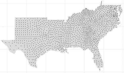
Table 1. Average number of connections by sample size and connection conditions.

	Sample Size
Connection Condition	196	400
${\mathbf{W}}_c^{\mathit{Low}}$	3.71	3.80
${\mathbf{W}}_c^{\mathit{Mid}}$	7.16	7.41
${\mathbf{W}}_c^{\mathit{High}}$	10.59	11.01
${\mathit{W}}_{\mathit{d}}^{\mathit{*}}$^1	37.91	55.71

1 The ${\mathit{W}}_{\mathit{d}}^{\mathit{*}}$ condition does not have neighbors. Every case is specified as a distance to every other case. Instead the mean row sum is displayed.

All simulation conditions were fully crossed. Under each simulation condition 500 data sets were generated (Muthén & Asparouhov, 2012). R version 3.5.4 (R Core Team, 2019) was used for the implementation of the study. The R package mvtnorm version 1.0-11 (Genz et al., 2019) was used for all multivariate data generation.

Analysis models for all studies

The general BARDSEM to analyze the data was specified as follows. The latent variable model was given by (11) $$\begin{array}{cc}\eta \hfill & =\rho \mathbf{W}\eta +{\gamma }_1{\xi }_1+{\gamma }_2{\xi }_2+{\omega }_{12}{\xi }_1{\xi }_2+\zeta \hfill \end{array}$$(11) and the measurement model by (12) $$\begin{array}{cc}\left(\begin{array}{c}{y}_1\\ y_2\\ y_3\end{array}\right)=\hfill & \left(\begin{array}{c}1\\ {\lambda }_{y2}\\ {\lambda }_{y3}\end{array}\right)·\eta +\left(\begin{array}{c}{ϵ}_1\\ {ϵ}_2\\ {ϵ}_3\end{array}\right)\hfill \end{array}$$(12) and (13) $$\begin{array}{cc}\left(\begin{array}{c}{x}_1\\ x_2\\ x_3\\ x_4\\ x_5\\ x_6\end{array}\right)=\hfill & \left(\begin{array}{cc}1& 0\\ {\lambda }_{x1}& 0\\ {\lambda }_{x2}& 0\\ 0& 1\\ 0& {\lambda }_{x3}\\ 0& {\lambda }_{x4}\end{array}\right)\left(\begin{array}{c}{\xi }_1\\ {\xi }_2\end{array}\right)+\left(\begin{array}{c}{\delta }_1\\ {\delta }_2\\ {\delta }_3\\ {\delta }_4\\ {\delta }_5\\ {\delta }_6\end{array}\right)\hfill \end{array}$$(13) where the first factor loading on each factor is set to one for identification. Prior specifications for the analysis models were given by (14) $$\begin{array}{cc}\mathit{\xi }\sim \hfill & \text{MVN}(\mathbf{0},\mathbf{\Phi })\hfill \\ {\gamma }_m\sim \hfill & N(0,1),\hspace{1em}\text{for}\mathrm{ }m=1\dots 2\hfill \\ {\omega }_{12}\sim \hfill & N(0,1)\hfill \\ \rho \sim \hfill & U[-1,1]\hfill \\ \alpha \sim \hfill & N(0,1)\hfill \\ \mathbf{\Phi }\sim \hfill & \text{LKJ}(2)\hfill \\ {\lambda }_{yj}\sim \hfill & N(0,1),\hspace{1em}\text{for}\mathrm{ }j=1\dots 2\hfill \\ {\lambda }_{xk}\sim \hfill & N(0,1),\hspace{1em}\text{for}\mathrm{ }k=1\dots 4\hfill \\ {\sigma }_{\xi p}\sim \hfill & C{(0,2.5)}^{+},\hspace{1em}\text{for}\mathrm{ }p=1\dots 2\hfill \\ {\sigma }_{\zeta }\sim \hfill & C{(0,2.5)}^{+}\hfill \\ {\sigma }_{ϵj}\sim \hfill & C{(0,2.5)}^{+},\hspace{1em}\text{for}\mathrm{ }j=1\dots 3\hfill \\ {\sigma }_{\delta k}\sim \hfill & C{(0,2.5)}^{+},\hspace{1em}\text{for}\mathrm{ }k=1\dots 6\hfill \end{array}$$(14) which follows the recommendations of LeSage and Parent (2007), Gelman et al. (2013), and Lee et al. (2007).

R version 3.5.4 (R Core Team, 2019), Stan version 2.18.0 (Stan Development Team, 2018), and Rstan version 2.19.2 (Stan Development Team, 2019) were used to conduct all analysis. All analysis models were designated to have four independent chains and 4,000 iterations, half of which was designated burn-in.

Outcomes

Performance of the analysis models was operationalized through convergence rates, parameter bias, and coverage. Convergence was considered acceptable when the $\widehat{R}$ estimate of a parameter was less than 1.05 (Gelman et al., 2013) and ESS > 400 (Vehtari et al., 2020)³. Bias was computed as the percent deviation of the population value from the mean posterior estimate as in $100\left(\frac{\text{Mean}\mathrm{ }\text{Posterior}\mathrm{ }\text{Estimate}-\text{Population}\mathrm{ }\text{Value}}{\text{Population}\mathrm{ }\text{Value}}\right).$ Population parameters that were 0 cannot be expressed as percent deviations; instead, they were computed as absolute bias: $\text{Mean}\mathrm{ }\text{Posterior}\mathrm{ }\text{Estimate}-\text{Population}\mathrm{ }\text{Value}.$ Coverage was calculated as the proportion of parameter values that fell within their respective 95% credible interval.

Results

The unabridged results for all parameters are provided in Appendix A. Figure 2 provides a graphical representation of the bias of the parameters of interest.

Figure 2. Bias plot of parameters of interest.

Model convergence rates were acceptable. Across simulation conditions and parameters convergence was consistently acceptable, the lowest observed convergence rate was observed in the ${\mathbf{W}}_d,$ ρ = 0, N = 400, conditions with 99.3% achieving $\widehat{R}>1.05$ and ESS ¿ 400.

Non-spatial parameters were consistently unbiased across all W conditions. Regarding ρ estimates, bias slightly increased as the number of connections in W increased. The most biased results were obtained in the fully saturated ${\mathbf{W}}_d$ condition in which estimates were consistently highly biased. In the ${\mathbf{W}}_d$ condition estimates of ρ were nearly always approximately 0, hence the negative direction of bias in the $\rho =0.3$ and 0.6 conditions. Regarding ${\mathbf{W}}_{\mathbf{c}}^{*}$ conditions, ${\mathbf{W}}_c^{\mathit{High}}$ exhibited the most biased estimates of ρ, under N = 196, ρ = 0 observed absolute bias is 6.76%, under population $\rho =0.3$ observed bias is 4.33%, under population $\rho =0.6$ observed bias is −5.09%. In the ${\mathbf{W}}_c^{\mathit{Mid}}$ condition observed bias is less. Under N = 196, ρ = 0 observed bias is 3.82%, under population $\rho =0.3$ observed bias is 0.91%, under population $\rho =0.6$ observed bias is −2.32%. Bias of ρ is lowest in the ${\mathbf{W}}_c^{\mathit{Low}}$ condition. Under ρ = 0 and sample size 196 the absolute bias of $\rho =2.11\%,$ under $\rho =0.3$ observed bias is 2.09%, and under $\rho =0.3$ observed bias is −1.63%. Bias decreased with sample size in all conditions.

Coverage rates were nearly identical across the ${\mathbf{W}}_c$ conditions. Coverage was consistently high for non-spatial parameters. Coverage of ρ was within the acceptable range under all conditions but lowest in the population ρ = 0 condition. Under ${\mathbf{W}}_c^{\mathit{Low}},$ N = 196, and a population parameter of ρ = 0, the coverage of ρ was 93%, rising to 95% when $\rho =0.6.$ Under ${\mathbf{W}}_c^{\mathit{High}},$ N = 196, and a population parameter ρ = 0, coverage rates lay at ρ is 92.2%, rising to 96.6% under $\rho =0.6.$ Coverage rates of ρ was higher in the N = 400 condition compared to N = 196.

Empirical example

The following example explores crime rate data obtained from the southern region of the United States (US) to demonstrate an applied use of the BARDSEM.

The US southern homicide data provides rates of crime for 1,412 counties in the southern US region in the year 1990. Aggregated by Land et al. (1990), the southern US homicide data has been frequently used as a typifying example in econometric and behavioral science literature (e.g. Kubrin & Weitzer, 2003; Morenoff, Sampson, & Raudenbush, 2001; Goodchild, Anselin, Appelbaum, & Harthorn, 2000). In the original data set, the variables of interest are homicide rate, Gini coefficient, and poverty rate. Additional variables were obtained by the Universal Crime Reporting (UCR) agency data tool website (Federal Bureau of Investigation, 2020). These variables are rates of aggravated assault, officer assault, burglary, theft (non vehicular), vehicle theft, and robbery. All rates are expressed as occurrences per 1,000 people within each county.⁴

Predicting violent crime

Identifying risk factors for violent crime rates at the societal level provides valuable information for behavioral scientists and policy makers. Research has established a link between financial inaccessibility and violent crime. As financial inaccessibility rises, violent crime rates increase (Deller & Deller, 2010).

Research has also noted a distinction in types of criminal acts. For example, violent crime and property crime are distinct constructs (Schreck, McGloin, & Kirk, 2009). A unified analysis which accounts for the latent multidimensional nature between these variables and the inherent spatial dependence is not available yet.

Research questions

Regions which have higher income inequality experience greater property and violent crime rates (Patterson, 1991). As a result, we find it reasonable to hypothesize an interaction effect between property crime and financial inaccessibility in the prediction of violent crime. Specifically, we anticipate that financial inaccessibility will moderate the relationship between property crime in its prediction of violent crime.

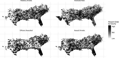
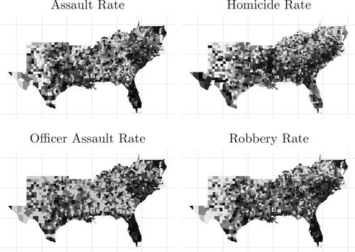
Prior research suggests nearer regions have more similar violent crime rates compared to further regions (Bernasco & Elffers, 2010). Thus, it is also reasonable to hypothesize the endogenous latent variable violent crime is spatially dependent. To illustrate this we present choropleth plots of the observed endogenous violent crime variables in Figure 3. If a variable is spatially dependent, the choropleth plot will yield observable patterns. In this example we see pockets of similar scores. Therefore, we hypothesize estimates of the spatial effect will be positive.

Figure 3. Choropleth plots of the observed endogenous variables. Darker shaded counties indicate higher values and lighter shaded counties have lower values relative to the mean of the sample.

Methods

Definitions and descriptive statistics

The variable homicide is the rate of murder and non-negligible manslaughter. Officer assault rate is the rate of aggravated assaults recorded against police. Assault is defined as violent physical assault with or without a weapon. Robbery rate is defined as the rate of nonviolent theft without the use of physical force or threats of force. Burglary is defined as illegal entry and theft. Theft is defined as nonviolent theft of personal property excluding motor vehicles. Motor vehicle theft rate is defined as theft or attempted theft of a vehicle. Unemployment rate is expressed as the percent of residents in a county who are unemployed despite looking for work. Poverty is the percent of families which are below the poverty threshold. The Gini coefficient is a measure of income inequality, where 0 indicates perfect income equality, and 1 represents perfect inequality (Dorfman, 1979).

Schreck et a. (2009) provide evidence suggesting violent and property crime are distinct factors. Evidence also suggests income inequality is a distinct factor (Deller & Deller, 2010; Rosenfeld, Baumer, & Messner, 2001). Therefore, we assume three distinct latent factors within the observed variables of interest: violent crime (VC); property crime (PC); and financial inaccessibility (FI). VC is comprised of homicide, officers assaulted, assault, and robbery rates. PC is comprised of burglary, theft, and vehicle theft rates. FI is comprised of unemployment rate, poverty rate, and Gini coefficient.⁵

Table 2 provides the sample means ($\overline{x}$), standard deviations (σ), minimum (Min.), and maximum (Max.) observed values for each variable.

Table 2. Extended US southern homicide data descriptive statistics for all counties.

Factor	Observed Variable	$\overline{x}$	σ	Min.	Max.
Violent Crime
	Homicide	0.09	0.07	0.00	0.64
	Officers Assault	0.21	0.31	0.00	3.52
	Assault	7.61	6.39	0.00	42.17
	Robbery	0.59	1.03	0.00	12.90
Property Crime
	Burglary	9.32	5.69	0.00	53.88
	Theft	18.97	13.64	0.00	92.69
	Vehicle Theft	2.00	2.11	0.00	24.43
Financial Inequality
	Unemployment	7.23	3.07	0.28	25.49
	Poverty	16.12	7.55	0.13	56.49
	Gini	0.39	0.03	0.26	0.53

$\overline{x}$ is the sample mean. σ is the sample standard deviation. Min. is the sample minimum. Max. is the sample maximum. All rates are expressed in occurrences by 1,000 people within each county.

Model and prior specification

The measurement model was specified using a simple structure for the items as described in Eqs. (12)(12) $$\begin{array}{cc}\left(\begin{array}{c}{y}_1\\ y_2\\ y_3\end{array}\right)=\hfill & \left(\begin{array}{c}1\\ {\lambda }_{y2}\\ {\lambda }_{y3}\end{array}\right)·\eta +\left(\begin{array}{c}{ϵ}_1\\ {ϵ}_2\\ {ϵ}_3\end{array}\right)\hfill \end{array}$$(12) and (13)(13) $$\begin{array}{cc}\left(\begin{array}{c}{x}_1\\ x_2\\ x_3\\ x_4\\ x_5\\ x_6\end{array}\right)=\hfill & \left(\begin{array}{cc}1& 0\\ {\lambda }_{x1}& 0\\ {\lambda }_{x2}& 0\\ 0& 1\\ 0& {\lambda }_{x3}\\ 0& {\lambda }_{x4}\end{array}\right)\left(\begin{array}{c}{\xi }_1\\ {\xi }_2\end{array}\right)+\left(\begin{array}{c}{\delta }_1\\ {\delta }_2\\ {\delta }_3\\ {\delta }_4\\ {\delta }_5\\ {\delta }_6\end{array}\right)\hfill \end{array}$$(13) . The latent variable model equation is given by: (15) $$\begin{array}{cc}VC\hfill & =\alpha +{\rho }_{VC}\mathbf{W}·VC+{\gamma }_{PC}·PC+{\gamma }_{FI}·FI+{\omega }_{PC·FI}·PC·FI+\zeta \hfill \end{array}$$(15)

We specified an endogenous spatial lag on the latent level, as the observed variable plots and prior research (Bernasco & Elffers, 2010) suggest spatial dependency in the observed items which transfers to the latent level. Prior choices follow the specifications from the Monte-Carlo study and are provided in Eq. 14(14) $$\begin{array}{cc}\mathit{\xi }\sim \hfill & \text{MVN}(\mathbf{0},\mathbf{\Phi })\hfill \\ {\gamma }_m\sim \hfill & N(0,1),\hspace{1em}\text{for}\mathrm{ }m=1\dots 2\hfill \\ {\omega }_{12}\sim \hfill & N(0,1)\hfill \\ \rho \sim \hfill & U[-1,1]\hfill \\ \alpha \sim \hfill & N(0,1)\hfill \\ \mathbf{\Phi }\sim \hfill & \text{LKJ}(2)\hfill \\ {\lambda }_{yj}\sim \hfill & N(0,1),\hspace{1em}\text{for}\mathrm{ }j=1\dots 2\hfill \\ {\lambda }_{xk}\sim \hfill & N(0,1),\hspace{1em}\text{for}\mathrm{ }k=1\dots 4\hfill \\ {\sigma }_{\xi p}\sim \hfill & C{(0,2.5)}^{+},\hspace{1em}\text{for}\mathrm{ }p=1\dots 2\hfill \\ {\sigma }_{\zeta }\sim \hfill & C{(0,2.5)}^{+}\hfill \\ {\sigma }_{ϵj}\sim \hfill & C{(0,2.5)}^{+},\hspace{1em}\text{for}\mathrm{ }j=1\dots 3\hfill \\ {\sigma }_{\delta k}\sim \hfill & C{(0,2.5)}^{+},\hspace{1em}\text{for}\mathrm{ }k=1\dots 6\hfill \end{array}$$(14) (weakly informative priors).

We used a contiguity W. Cases were considered neighbors if they shared a common border. This was done to align with the concept that crime was more likely to spillover to neighboring counties with shared borders. Figure 4 provides a visual representation of the connections representing the W utilized.

Figure 4. Connection visualization of W representation. Cases with lines connecting their center-points were considered neighbors.

The analysis was conducted using R version 3.5.4 (R Core Team, 2019), Stan version 2.18.0 (Stan Development Team, 2018), and Rstan version 2.19.2 (Stan Development Team, 2019). Four independent chains were specified. Chains ran for 4,000 iterations each, half of which were designated burn-in. All variables were standardized prior to analysis.

Results

Results for the BARDSEM are given in Table 3. All parameters of interest met the convergence criteria of $\widehat{R}<1.01$ and ESS ¿ 400. All results are presented as 95% credible intervals. Factor loadings were all high and positive. The spatial effect ${\widehat{\rho }}_{VC}$ fell in a credible interval of (0.68, 0.98). The latent structural coefficients were non-zero with ${\widehat{\gamma }}_{FI}$ within (0.05, 0.09), ${\widehat{\gamma }}_{PC}$ within (0.39,0.51), and the latent interaction effect ${\widehat{\omega }}_{FI·PC}$ in (0.00,0.05). The covariance between the latent factors was within (−0.11, −0.04), and reflected a small negative correlation.

Table 3. Results table for the BARDSEM analysis of the US southern homicide data set.

	$\overline{\widehat{\theta }}$	2.5%	97.5%	ESS	$\widehat{R}$
ρV C	0.87	0.68	0.98	4585	1.00
α	0.00	−0.05	0.05	1623	1.00
γ FI	0.07	0.05	0.09	2026	1.00
γ PC	0.45	0.39	0.51	812	1.01
${\omega }_{PC·FI}$	0.02	0.00	0.05	2563	1.00
${\lambda }_{\text{Robbery}}$	2.07	1.83	2.35	686	1.01
${\lambda }_{\text{Officers}\mathrm{ }\text{Assaulted}}$	1.21	1.02	1.43	963	1.01
${\lambda }_{\text{Assault}}$	2.03	1.79	2.32	731	1.01
${\lambda }_{\text{Gini}}$	1.24	1.17	1.30	2768	1.00
${\lambda }_{\text{Poverty}}$	1.28	1.22	1.35	3017	1.00
${\lambda }_{\text{Theft}}$	1.06	1.01	1.11	5112	1.00
${\lambda }_{\text{Motor}\mathrm{ }\text{Vehicle}\mathrm{ }\text{Theft}}$	0.95	0.90	1.01	4301	1.00
${\varphi }_{PC,FI}$	−0.07	−0.11	−0.04	668	1.01
${\varphi }_{PC}$	0.72	0.65	0.80	1523	1.00
${\varphi }_{FI}$	0.56	0.50	0.63	964	1.00

$\overline{\widehat{\theta }}$ are the means, and 2.5% and 95.5% are the respective percentiles of the posterior distribution. ESS is the effective sample size. $\widehat{R}$ the coefficients estimated $\widehat{R}$ value for assessing convergence,values of 1.01 are rounded and at 3 decimal places are < 1.01. $\text{Fin}.\text{Accessibility}·\text{Prop}.\text{Crime}$ provides the interaction term of Property Crime and Financial Accessibility.

Model interpretation

To interpret the structural effects, marginal direct, indirect, and total spillover were calculated using in Eq. 6(6) $${\partial }_{\eta }/{\partial }_{\xi }^{q\prime }={({\mathbf{I}}_N-\widehat{\rho }\mathbf{W})}^{-1}{\mathit{I}}_N({\widehat{\gamma }}_m+{\widehat{\omega }}_{12}{S}_q)$$(6) . A convenient means of calculating these effects in the Bayesian framework is the ability to include spillover calculations in the model and thus provide posterior distributions for inference. Table 4 provides the means and 95% credible intervals for the marginal direct, indirect, and total spillover of PC at marginal values of $FI=(-2,-1,0,1,2).$

Table 4. Marginal direct, indirect, and total spillover effects and their 95% credible intervals (in brackets) for γ_PC conditional on different values for FI.

FI	Direct	Indirect	Total
–2	0.28 (0.25, 0.32)	1.25 (1.11, 1.43)	1.38 (1.31, 1.52)
–1	0.30 (0.24, 0.33)	1.30 (1.15, 1.51)	1.58 (1.41, 1.81)
0	0.28 (0.26, 0.34)	1.42 (1.18, 1.52)	1.69 (1.51, 1.76)
+1	0.31 (0.23, 0.36)	1.51 (1.27, 1.63)	1.80 (1.57, 2.03)
+2	0.32 (0.22, 0.37)	1.59 (1.31, 1.69)	1.91 (1.63, 2.18)

The spillover effects provide us with a means of interpreting the spatial estimate ${\widehat{\rho }}_{VC}$ (0.68, 0.98) in the context of the variables in space.

Direct spillover

The mean posterior estimate of the direct spillover of PC given low FI = − 2 was 0.28. This means that when county i sees an increase of one SD on PC and given FI = − 2, all $\ne i$ counties see an average increase of 0.28 SD in VC. If FI was high ($FI=+2$), the spillover effect for PC was 0.32. This means the model expected a greater spatial spillover of VC from increases in PC when the original county has more FI.

Indirect spillover

The mean posterior estimate of the indirect spillover of PC given FI = − 2 was 1.25. This means a one SD increase in all counties $\ne i$ and given FI = − 2 would result in an expected 1.25 standard deviation increase in VC on average in county i. Again, we see that if FI was higher ($FI=+2$), the indirect spillover was higher with an estimate of 1.59.

Total spillover

The mean posterior estimate of the total spillover of PC given FI = − 2 was 1.38. This means the model expects a 1.38 SD increase in VC on average in all counties when all counties see a one SD increase in PC and given FI = − 2. The spillover increased to 1.91 when the marginal value of FI was high ($FI=+2$).

Interpretation of region of interest

To provide an example of interpretations for specific regions of interest, we picked an arbitrary county: Mills County, Texas. We computed the CPDM (see Eq. 7(7) $${\partial }_{\eta }/{\partial }_{\xi }^{\prime }={({\mathbf{I}}_N-\widehat{\rho }\mathbf{W})}^{-1}{\mathit{I}}_N({\widehat{\gamma }}_m+{\widehat{\omega }}_{12}{\widehat{\xi }}_{im})$$(7) ) using the estimated main and interaction effects (${\widehat{\gamma }}_{PC},{\widehat{\omega }}_{PC·FI}$) as well as the estimate for Mills County’s factor score $\widehat{FI}.$ By taking the off-diagonal element associated with Mills County from the CPDM we see that when all counties included in the analysis except Mills see an increase in the PC factor of one SD, Mills County itself is expected to see a 0.31 SD increase in VC. Mills County has six first order neighbors: Comanche, Brown, Hamilton, San Saba, and Lampasas County. Looking at the associated elements of the CPDM we see that a one SD increase in PC in Mills County is associated with expected increases of 0.098 SD for Comanche, 0.076 SD for Brown, 0.075 SD for San Saba, 0.085 SD for Lampasas, and 0.089 SD for Hamilton. Figure 5 provides a visualization of this spillover to higher order neighbors of Mills County.

Figure 5. Visualization of spillover for an increase in PC of 1 SD in Mills County Texas, denoted as a triangle. Expected increases less than 0.005 are suppressed.

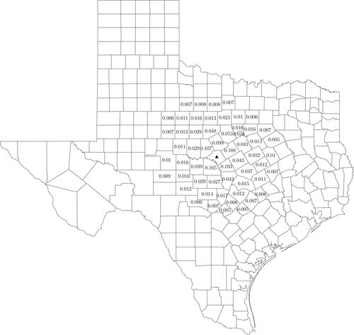
Visual inspection of the spillover plot shows how the impact of Mills County diminishes in space. The average expected increase in first order neighbors to Mills County is 0.1 SD, at the second order neighbor level the average expected increase is reduced to 0.033 SD. By the third order neighbors the spatial spillover approaches zero, with an average expected increase in VC of 0.01 SD.

Summary

In the example we showed that VC is spatially dependent, this implies changes in PC and FI in nearby counties spills over to one another. The non-zero latent interaction effect between PC and FI suggested a a nonlinear relationship with VC. Investigating the effects together revealed that counties with higher FI were expected to have more spatial spillover of VC if PC increases.

Discussion

The BARDSEM provides a framework for estimating SEM with spatially or socially dependent data. These models allow researchers to estimate latent variables from sets of observed indicators while simultaneously providing a means to estimate spatial or social dependence effects. In spatial settings (as shown with the violent crime example), the addition of latent variables provides an extension to account for multi-dimensional societal constructs. In social network contexts, the BARDSEM can model the complex intricacies of networks of agents and lends itself well to the psychological tradition of measuring person level constructs as latent variables. Instead of making predictions on and with univariate variables, the BARDSEM framework allows network scientists to predict complex unobserved features. This is a major advantage over potential dimension reduction alternatives like sum-scores (Bollen, 1989; DiStefano, Zhu, & Mindrila, 2009).

Monte Carlo study

The goal of the Monte-Carlo study was to assess the BARDSEM performance under different spatial effect magnitudes, sample sizes, and W specifications. The primary finding is that the BARDSEM accurately estimates both spatial and non-spatial parameters under non-fully saturated W specifications. This supports existing research in regression contexts that high connectivity W specifications negatively bias spatial effects (Smith, 2009) and may require higher sample sizes to maintain accuracy (Stakhovych & Bijmolt, 2009).

Empirical example

The empirical example was intended to provide an example of the rich interpretations of coefficients provided by the BARDSEM. The combination of the measurement model, latent interaction, and spatial effect, provide a unique understanding of violent crime. We showed that the anticipated spatial spillover in violent crime due to an increase in property crime was higher in counties with higher financial inaccessibility. In addition the results suggest a strong spatial effect of violent crime. This effect was explored by using spillover estimates to depict the interaction of space and the exogenous latent predictors. Recall that our indirect spillover estimates provide us with evidence that increases in property crime in neighboring counties is associated with increases in violent crime in the original county. This increase is stronger when financial inequality is higher. Further information is obtained when we extrapolate impact calculations to a region of interest, as we did with Mills County. Recall that an increase of 1 SD in property crime in Mills County coincided with an expected 0.31 SD increase in violent crime in Mills County. This was because the model suggests Mills County’s increase in property crime led to an expected increased violent crime in its neighbors, which in turn spilled back to Mills County.

Practical recommendations

The BARDSEM exhibits unbiased estimation properties in the sample sizes tested when parsimonious representations of W were used. Here we provide brief recommendations for its application.

Sample size requirements appear similar to general recommendations in latent variable modeling (Westland, 2010) but is connected to W choice. Following the advice of Stakhovych and Bijmolt (2009) in situations with lower than optimal sample size, select a parsimonious weight matrix specification. In spatial settings this may mean simply opting to determine cutoff rules for determining neighbors (e.g. shared borders, but not shared corners). In network settings a cutoff threshold can be specified to trim weak connections between cases. This advice reinforces that of Griffith (1996) in regression settings.

Regarding priors, if researchers aim to directly interpret or compare ${\rho }_{\eta }$ estimates we recommend a row normalized W in conjunction with ${\rho }_{\eta }\sim$ Uniform(-1,1). In studies with high sample sizes and strong evidence suggesting a positive spatial relationship, setting a lower bound of 0 can substantially save computation time.

Limitations

The Monte-Carlo BARDSEM we investigated had a limited amount of complexity. Additional complexity can be induced by including more spatial effects, more latent variables, or more complex model specifications. For simplicity we used parallel items during Monte-Carlo data generation (uniform reliabilities) which is not achievable for many psychological constructs⁶. Theoretically, different priors could have been investigated. Here we used weakly informative priors. With the given sample sizes 196 and 400, the actual choice of priors should not have much of an impact, but might be more crucial for smaller effect sizes.

Regarding the empirical example, only one W specification was implemented. To align with the concept that crime is likely to spillover to neighboring counties and not directly to distant ones a contiguity W was used. The choice to not explore other potential specifications of W assumes the spatial process follows this logic. Further, we show a parsimonious representation to be the most accurate at recovering the spatial parameter and was thus chosen for the example.

Regarding the BARDSEM itself, the use of fully saturated W specifications is problematic. Theory may suggest that each case directly impacts all other cases and indirectly impacts all other cases through spillover. To accommodate this in theoretically a distance W could be used. A fully saturated ${\mathbf{W}}_D^{*}$ reflected this in the Monte-Carlo study. This representation was biased under the sample sizes tested in the and thus should not be used.

Regarding the BARDSEM assumptions, most notably conditional independence is worth mentioning. The BARDSEM can be broadly applied, thus, in some situations this assumption is more plausible than others. It may be the case that un-modelded spatial dependence may remain and bias results. The granularity of the spatial information may not fully account for the dependence. For example, measurement of cultural variables using countries in Europe as spatial units (as compared to finer spatial sub-regions) will likely not capture the finer details of the spatial relationship. This situation is akin to a poor measurement tool in that the spatial units do not accurately capture the spatial process, thus masking the effect of interest. An alternative way of thinking about this problem is with repeated measures situations. If a researcher aims to measure the trajectories of human weight fluctuations and seasonality, measuring twice per year will not provide granular enough measurements to detect the intended effect.

Next, in the models explored we assumed that W is observable and known, which may not always be true. Folmer and Oud (2008) discussed a method for predicting W which can theoretically provide an alternative to exogenous specifications of W.

Finally, spatial or other forms of dependence may exhibit themselves not only in the endogenous variable but also in the predictors or error terms of models. In econometric literature with observed variables this is addressed in different ways. Instrumental variables or additional spatial lags provide solutions to these issues. The BARDSEM can accommodate instrumental variables approach, but not additional spatial lags.

Future research

The BARDSEM shows promising performance and should be explored further. Specifically, The BARDSEM should be generalized to more situations than described in this paper. First, to address the issues with the fully saturated ${\mathit{W}}_{\mathit{D}}^{\mathit{*}},$ it is possible that a vastly higher sample size is necessary to determine if ρ can be accurately estimated. The boundaries of this scenario should be explored further.

Next, in some situations it may be unrealistic to assume that a single scalar summary accurately measures the population level spatial process. The BARDSEM could be extended to include a random effect of ${\rho }_{\eta }$ at the structural level (Rabe-Hesketh, Skrondal, & Zheng, 2007), which allows variation in the magnitude of the effect of ${\rho }_{\eta }$ across different clusters of spatial units (e.g., counties in states). Alternatively, multi-group latent variable models (like the MIMIC model (Jöreskog, 1971)) could be applied to account for variations in ρ by a known grouping factor.

Next, it could be reasonable to assume that spatial dependence varies across several known or unknown groups (e.g., rural vs metropolitan areas). Latent class analysis provides a means to extend the BARDSEM to account for such heterogeneity in spatial dependency.

Finally, modern data collection methods (e.g.,such as mobile phone apps) allow researchers to collect dynamic psychologically relevant data (e.g., attitudes, feelings, and cognitive performances) in field experiments with high external validity. Further, dynamic spatial information can be collected where the participants respond to the questions or tasks. Extensions of the BARDSEM to account for dynamic changes in spatial or social dependency are necessary to model such data (e.g., using dynamic latent class structural equation models as in: Asparouhov et al., 2017; Asparouhov, Hamaker, & Muthén, 2018; Kelava & Brandt, 2019).

Conclusion

The BARDSEM is a promising addition to the set of methods for analyzing multivariate spatial or network dependent data. As network science grows, interest in dependent methodology has increased. Current approaches restrict the types of data that can be analyzed as methods are typically constrained to observed variables. The BARDSEM provides a solution to this problem. Researchers in the social sciences frequently investigate complex relationships between three or more variables. The ability to simultaneously accommodate latent interaction effects with dependent spillover effects provides a means to match methodological approaches and rich interpretations to complex theory.

Article information

Conflict of interest disclosures: Each author signed a form for disclosure of potential conflicts of interest. No authors reported any financial or other conflicts of interest in relation to the work described.

Ethical principles: The authors affirm having followed professional ethical guidelines in preparing this work. These guidelines include obtaining informed consent from human participants, maintaining ethical treatment and respect for the rights of human or animal participants, and ensuring the privacy of participants and their data, such as ensuring that individual participants cannot be identified in reported results or from publicly available original or archival data.

Funding: No funding provided.

Role of the funders/sponsors: None of the funders or sponsors of this research had any role in the design.

Acknowledgments: The authors would like to thank the Multivariate Behavioral Research associate editor Dr. Sarah Depaoli and the review team for their comments on prior versions of this manuscript. The ideas and opinions expressed herein are those of the authors alone, and endorsement by the authors' institution is not intended and should not be inferred.

Data availability statement

The arrest data that support the findings of this study are openly available in the” ICPSR” database at” https://doi.org/10.3886/ICPSR09785.v1”, reference code” ICPSR09785”.

The homicide data that support the findings of this study are openly available in the” GeoDa Data” repository at” https://geodacenter.github.io/data-and-lab/south/”, reference code” south”.

Notes

1 Due to the continuous latent variables, marginal slope values are used as a means to explain the effect of a latent variable of interest dependent on different levels of the moderating latent variable. One term for this process is” probing interaction effects”. We suggest -2, -1, 0, 1, and 2 $\times SD(\xi )$

2 See Appendix B.1 for more details about CPDM.

3 $\widehat{R}$ was computed using the metric described by Vehtari, Gelman, Simpson, Carpenter, and Bürkner (2020)

4 Due to some incongruities in the county cataloguing system (FIPS codes), 2 counties were omitted from the analysis resulting in a total N of 1,410.

5 Note that these (statistical) factors can be seen as composites. For the sake of simplicity and due to the illustrative character of this example, standard reflective measurement models were used and not formative factor models (additionally see the discussion and recommendation to use reflective measurement models in Howell, Breivik, & Wilcox, 2007).

6 We conducted a small scale Monte-Carlo study to test if non-parallel items impacted model performance. Our results suggest there is not a systematic relationship between item reliabilities and the bias, or coverage of the BARDSEM parameter estimates.

Appendix A

Results from the simulation study

Table A1. Results table for Monte-Carlo study.

				ρ = 0			$\rho =0.3$			$\rho =0.6$
${\mathbf{W}}^{*}$	N		θ	$\overline{\widehat{\theta }}$	$\mathit{Bias}(\theta )\%$	Coverage	$\overline{\widehat{\theta }}$	$\mathit{Bias}(\theta )\%$	Coverage	$\overline{\widehat{\theta }}$	$\mathit{Bias}(\theta )\%$	Coverage
${\mathbf{W}}_C^{\mathit{low}}$
196
		ρ	0.00	0.02	2.11	93.00	0.31	2.09	95.20	0.59	−1.63	95.00
		α	0.00	0.00	−0.28	95.60	0.00	−0.07	94.80	0.01	1.02	94.80
		γ 1	0.30	0.30	−0.78	96.00	0.30	0.48	96.20	0.29	−1.76	93.80
		γ 2	0.30	0.30	1.55	95.20	0.30	−0.23	95.20	0.30	0.89	96.00
		ω 12	0.15	0.16	4.97	96.00	0.16	4.42	94.60	0.15	−1.49	94.40
		${\sigma }_{\delta 1}$	0.50	0.50	0.57	94.20	0.50	0.94	94.80	0.50	0.06	96.40
		${\sigma }_{\delta 2}$	0.50	0.50	0.00	94.60	0.50	0.16	95.40	0.50	0.48	94.00
		${\sigma }_{\delta 3}$	0.50	0.50	0.43	95.20	0.50	0.39	94.80	0.50	0.20	94.40
		${\sigma }_{\delta 4}$	0.50	0.50	0.38	93.80	0.50	0.73	93.40	0.50	0.39	94.60
		${\sigma }_{\delta 5}$	0.50	0.50	0.80	95.00	0.50	0.07	95.40	0.50	0.87	94.00
		${\sigma }_{\delta 6}$	0.50	0.50	0.84	94.60	0.50	0.81	94.60	0.50	0.61	94.20
		${\sigma }_{ϵ1}$	0.50	0.50	0.59	94.60	0.50	0.98	94.40	0.50	0.02	96.80
		${\sigma }_{ϵ2}$	0.50	0.50	0.23	96.80	0.50	0.00	95.60	0.50	0.22	94.60
		${\sigma }_{ϵ3}$	0.50	0.50	0.28	95.20	0.50	0.08	94.80	0.50	0.93	95.00
		${\sigma }_{\zeta }$	1.00	1.01	1.73	82.80	1.01	−0.89	78.80	1.00	−6.23	66.40
		${\varphi }_{1,1}$	1.00	1.00	−0.34	94.20	1.00	0.43	94.80	1.00	0.02	93.60
		${\varphi }_{2,2}$	1.00	1.00	0.08	94.20	1.00	0.30	94.00	1.00	0.30	94.20
		${\tau }_{x_1}$	0.00	0.00	−0.12	96.00	0.00	−0.22	94.40	0.00	−0.40	96.40
		${\tau }_{x_2}$	0.00	0.00	0.15	95.80	0.00	−0.48	95.20	0.00	0.07	96.60
		${\tau }_{x_3}$	0.00	0.00	−0.04	96.00	0.00	−0.15	94.80	0.00	−0.01	96.00
		${\tau }_{x_4}$	0.00	0.00	−0.19	95.40	0.00	−0.23	94.40	0.00	0.02	92.80
		${\tau }_{x_5}$	0.00	0.00	−0.31	96.20	0.00	−0.04	96.00	0.00	0.28	93.80
		${\tau }_{x_6}$	0.00	−0.01	−0.54	96.00	0.00	−0.01	96.20	0.00	0.17	94.20
		${\tau }_{y_2}$	0.00	0.00	0.03	94.80	0.00	0.21	96.40	0.00	−0.05	95.40
		${\tau }_{y_3}$	0.00	0.00	0.08	94.80	0.00	−0.09	96.80	0.00	0.04	95.60
		${\lambda }_{x_2}$	1.00	1.01	1.04	95.20	1.01	0.73	94.00	1.00	0.35	94.20
		${\lambda }_{x_3}$	1.00	1.01	0.98	95.00	1.01	0.70	94.40	1.01	0.94	94.00
		${\lambda }_{x_4}$	1.00	1.00	0.45	94.00	1.00	0.40	94.60	1.01	0.75	94.40
		${\lambda }_{x_5}$	1.00	1.00	0.34	94.80	1.00	0.41	94.60	1.01	0.75	95.80
		${\lambda }_{y_2}$	1.00	1.00	−0.15	96.40	1.00	−0.42	94.80	1.00	−0.31	95.00
		${\lambda }_{y_3}$	1.00	1.00	−0.17	95.60	1.00	−0.24	95.80	1.00	−0.18	97.00
400
		ρ	0.00	0.02	2.08	95.60	0.30	0.47	94.40	0.60	−0.67	95.00
		α	0.00	0.00	−0.10	95.00	0.00	−0.35	94.60	0.00	0.04	95.20
		γ 1	0.30	0.30	1.06	96.60	0.30	1.08	95.60	0.30	−0.29	95.40
		γ 2	0.30	0.30	0.31	94.80	0.30	0.94	95.20	0.30	0.04	96.60
		ω 12	0.15	0.15	−0.26	95.60	0.16	4.72	94.60	0.15	0.43	94.80
		${\sigma }_{\delta 1}$	0.50	0.50	0.35	95.80	0.50	0.19	95.20	0.50	0.10	95.80
		${\sigma }_{\delta 2}$	0.50	0.50	0.32	94.40	0.50	0.79	96.20	0.50	0.48	95.20
		${\sigma }_{\delta 3}$	0.50	0.50	0.30	96.60	0.50	0.12	95.80	0.50	0.43	94.40
		${\sigma }_{\delta 4}$	0.50	0.50	0.83	93.80	0.50	0.34	95.80	0.50	0.17	96.20
		${\sigma }_{\delta 5}$	0.50	0.50	0.13	96.00	0.50	0.10	94.00	0.50	0.18	92.60
		${\sigma }_{\delta 6}$	0.50	0.50	0.02	93.80	0.50	0.03	93.80	0.50	0.43	94.60
		${\sigma }_{ϵ1}$	0.50	0.50	0.20	95.60	0.50	−0.06	94.20	0.50	0.09	93.80
		${\sigma }_{ϵ2}$	0.50	0.50	0.45	94.60	0.50	0.53	94.00	0.50	0.38	94.20
		${\sigma }_{ϵ3}$	0.50	0.50	−0.15	94.80	0.50	0.15	95.20	0.50	0.69	95.60
		${\sigma }_{\zeta }$	1.00	1.01	0.09	81.20	1.00	−1.93	80.60	1.00	−7.69	51.80
		${\varphi }_{1,1}$	1.00	1.01	0.64	96.00	1.00	0.30	95.20	1.00	0.35	94.60
		${\varphi }_{2,2}$	1.00	1.00	0.26	95.00	1.00	0.02	95.40	1.00	−0.22	93.80
		${\tau }_{x_1}$	0.00	0.00	0.21	95.40	0.00	−0.16	94.40	0.00	0.14	95.60
		${\tau }_{x_2}$	0.00	0.00	0.11	95.00	0.00	−0.27	94.80	0.00	−0.04	95.40
		${\tau }_{x_3}$	0.00	0.00	0.23	94.60	0.00	−0.19	94.60	0.00	0.26	95.80
		${\tau }_{x_4}$	0.00	0.00	−0.01	96.60	0.00	0.43	94.20	0.00	−0.27	95.00
		${\tau }_{x_5}$	0.00	0.00	−0.09	95.20	0.00	0.31	93.40	0.00	−0.26	96.60
		${\tau }_{x_6}$	0.00	0.00	0.00	94.00	0.00	0.24	95.20	0.00	−0.28	95.60
		${\tau }_{y_2}$	0.00	0.00	−0.23	94.80	0.00	0.27	96.00	0.00	−0.26	96.00
		${\tau }_{y_3}$	0.00	0.00	−0.08	96.20	0.00	0.40	93.80	0.00	−0.13	94.60
		${\lambda }_{x_2}$	1.00	1.00	0.11	96.00	1.00	0.10	95.60	1.00	0.36	96.20
		${\lambda }_{x_3}$	1.00	1.00	0.12	95.20	1.00	0.23	96.60	1.00	−0.07	95.80
		${\lambda }_{x_4}$	1.00	1.00	0.07	96.40	1.00	0.25	94.40	1.00	0.34	92.60
		${\lambda }_{x_5}$	1.00	1.00	0.31	95.00	1.00	0.29	94.20	1.00	−0.10	95.20
		${\lambda }_{y_2}$	1.00	1.00	−0.43	93.40	1.00	−0.17	95.20	1.00	−0.16	96.40
		${\lambda }_{y_3}$	1.00	1.00	−0.20	95.20	1.00	−0.29	94.40	1.00	−0.35	95.00
${\mathbf{W}}_C^{\mathit{mid}}$
196
		ρ	0.00	0.04	3.82	92.60	0.30	0.91	95.00	0.59	−2.32	97.00
		α	0.00	0.00	0.20	96.20	0.00	0.13	94.00	0.00	0.35	95.40
		γ 1	0.30	0.30	0.89	95.00	0.30	1.52	96.60	0.29	−1.82	95.00
		γ 2	0.30	0.30	0.37	95.40	0.30	−0.45	96.00	0.30	−0.78	94.80
		ω 12	0.15	0.16	3.64	96.20	0.15	2.47	95.20	0.15	0.10	95.20
		${\sigma }_{\delta 1}$	0.50	0.50	0.53	95.20	0.50	0.78	94.80	0.50	−0.08	94.00
		${\sigma }_{\delta 2}$	0.50	0.50	0.74	94.20	0.50	0.70	93.60	0.51	1.07	94.60
		${\sigma }_{\delta 3}$	0.50	0.50	0.42	95.60	0.50	0.20	95.40	0.50	0.46	94.80
		${\sigma }_{\delta 4}$	0.50	0.50	0.27	94.20	0.50	0.06	94.60	0.50	0.10	93.40
		${\sigma }_{\delta 5}$	0.50	0.50	0.24	95.00	0.50	0.11	96.00	0.50	−0.10	94.60
		${\sigma }_{\delta 6}$	0.50	0.50	−0.10	95.60	0.50	0.58	94.80	0.50	0.79	95.20
		${\sigma }_{ϵ1}$	0.50	0.50	0.23	94.80	0.50	0.00	94.80	0.50	0.28	95.40
		${\sigma }_{ϵ2}$	0.50	0.51	1.73	95.20	0.50	0.66	94.20	0.50	0.02	94.80
		${\sigma }_{ϵ3}$	0.50	0.50	0.81	93.20	0.50	0.70	95.40	0.50	0.88	95.20
		${\sigma }_{\zeta }$	1.00	1.01	1.62	82.40	1.01	0.70	83.00	1.00	−2.71	78.60
		${\varphi }_{1,1}$	1.00	0.99	−0.52	95.80	1.00	0.15	93.60	1.00	0.43	94.60
		${\varphi }_{2,2}$	1.00	1.00	0.40	93.80	1.01	1.02	95.20	1.00	0.39	93.80
		${\tau }_{x_1}$	0.00	0.00	−0.10	92.20	0.00	−0.11	94.80	0.00	−0.13	95.00
		${\tau }_{x_2}$	0.00	0.00	0.14	94.80	0.00	0.03	96.00	0.00	−0.47	96.00
		${\tau }_{x_3}$	0.00	−0.01	−0.58	93.40	0.00	0.10	96.60	0.00	0.12	95.40
		${\tau }_{x_4}$	0.00	0.00	−0.16	94.80	0.00	−0.26	96.20	0.01	0.69	95.40
		${\tau }_{x_5}$	0.00	0.00	−0.33	96.20	0.00	−0.17	93.80	0.01	0.70	95.20
		${\tau }_{x_6}$	0.00	0.00	−0.30	94.00	0.00	−0.20	95.20	0.01	0.68	93.40
		${\tau }_{y_2}$	0.00	0.00	0.27	95.20	0.00	−0.01	96.40	0.00	−0.03	96.20
		${\tau }_{y_3}$	0.00	0.00	0.07	96.00	0.00	0.12	95.40	0.00	−0.01	94.60
		${\lambda }_{x_2}$	1.00	1.01	0.59	94.80	1.01	0.81	95.40	1.01	0.68	93.80
		${\lambda }_{x_3}$	1.00	1.00	0.49	95.00	1.01	1.21	95.60	1.01	0.54	95.60
		${\lambda }_{x_4}$	1.00	1.00	0.44	95.60	1.00	0.30	95.60	1.00	0.11	94.60
		${\lambda }_{x_5}$	1.00	1.01	0.52	96.40	1.00	0.21	93.80	1.00	−0.11	96.00
		${\lambda }_{y_2}$	1.00	0.99	−0.54	93.80	0.99	−0.74	94.80	1.00	0.28	95.80
		${\lambda }_{y_3}$	1.00	0.99	−0.60	95.80	0.99	−0.68	92.80	1.00	−0.33	94.60
400
		ρ	0.00	0.03	2.61	94.60	0.31	3.45	94.00	0.60	0.60	95.00
		α	0.00	0.00	−0.11	92.60	0.00	0.30	94.20	0.00	−0.02	94.60
		γ 1	0.30	0.30	−0.98	95.20	0.30	−0.73	97.80	0.30	0.76	95.20
		γ 2	0.30	0.30	0.12	96.40	0.30	0.72	95.00	0.30	0.05	96.20
		ω 12	0.15	0.15	−0.16	94.20	0.15	0.56	92.80	0.14	−5.55	95.00
		${\sigma }_{\delta 1}$	0.50	0.50	0.09	96.00	0.50	0.11	95.20	0.50	0.40	93.20
		${\sigma }_{\delta 2}$	0.50	0.50	0.11	92.80	0.50	0.45	95.40	0.50	0.01	94.80
		${\sigma }_{\delta 3}$	0.50	0.50	0.46	95.00	0.50	−0.06	95.00	0.50	0.20	93.60
		${\sigma }_{\delta 4}$	0.50	0.50	0.10	95.40	0.50	0.20	94.20	0.50	0.75	94.00
		${\sigma }_{\delta 5}$	0.50	0.50	0.11	96.80	0.50	−0.34	94.40	0.50	0.12	95.00
		${\sigma }_{\delta 6}$	0.50	0.50	0.25	94.80	0.50	0.48	94.00	0.50	−0.10	94.00
		${\sigma }_{ϵ1}$	0.50	0.50	−0.08	95.20	0.50	−0.24	94.80	0.50	−0.14	94.20
		${\sigma }_{ϵ2}$	0.50	0.50	0.35	94.80	0.50	0.07	94.00	0.50	0.37	95.40
		${\sigma }_{ϵ3}$	0.50	0.50	0.21	93.40	0.50	0.43	95.60	0.50	0.32	93.20
		${\sigma }_{\zeta }$	1.00	1.00	0.71	78.60	1.00	−0.40	79.80	1.01	−4.17	71.60
		${\varphi }_{1,1}$	1.00	1.00	−0.06	93.80	1.00	0.17	95.00	1.00	−0.12	95.60
		${\varphi }_{2,2}$	1.00	1.00	0.13	95.60	1.00	0.11	94.40	1.00	0.28	93.80
		${\tau }_{x_1}$	0.00	0.00	0.33	94.20	0.00	−0.05	95.20	0.00	−0.09	95.60
		${\tau }_{x_2}$	0.00	0.00	0.25	93.40	0.00	−0.10	94.40	0.00	−0.14	93.20
		${\tau }_{x_3}$	0.00	0.00	0.22	94.80	0.00	0.26	95.40	0.00	−0.17	94.60
		${\tau }_{x_4}$	0.00	0.00	−0.20	94.00	0.00	−0.08	95.00	0.00	0.00	95.80
		${\tau }_{x_5}$	0.00	0.00	−0.48	94.20	0.00	−0.12	96.00	0.00	0.02	96.40
		${\tau }_{x_6}$	0.00	−0.01	−0.63	92.60	0.00	0.03	95.40	0.00	0.13	95.20
		${\tau }_{y_2}$	0.00	0.00	−0.01	94.80	0.00	0.06	96.00	0.00	0.00	95.00
		${\tau }_{y_3}$	0.00	0.00	0.12	95.40	0.00	−0.01	94.40	0.00	−0.35	94.60
		${\lambda }_{x_2}$	1.00	1.00	0.24	94.80	1.00	0.15	94.20	1.00	0.49	97.00
		${\lambda }_{x_3}$	1.00	1.00	0.24	95.20	1.00	0.13	95.60	1.00	0.44	96.20
		${\lambda }_{x_4}$	1.00	1.00	0.04	93.80	1.00	0.02	95.40	1.00	0.39	93.80
		${\lambda }_{x_5}$	1.00	1.00	0.08	94.00	1.00	−0.06	97.00	1.00	0.47	93.40
		${\lambda }_{y_2}$	1.00	1.00	−0.05	95.60	1.00	−0.21	97.80	1.00	−0.38	95.00
		${\lambda }_{y_3}$	1.00	1.00	0.09	96.20	1.00	−0.12	95.60	1.00	−0.32	94.40
${\mathbf{W}}_C^{\mathit{high}}$
196
		ρ	0.00	0.07	6.76	92.20	0.31	4.33	94.40	0.57	−5.09	96.60
		α	0.00	0.01	0.62	95.00	0.00	−0.26	96.20	0.01	0.65	94.80
		γ1	0.30	0.30	0.81	95.00	0.30	0.48	96.00	0.30	0.55	95.00
		γ2	0.30	0.31	2.35	95.60	0.30	1.25	95.20	0.30	−0.30	94.40
		ω12	0.15	0.15	0.19	93.80	0.15	2.47	94.60	0.15	1.96	95.40
		${\sigma }_{\delta 1}$	0.50	0.50	0.34	94.80	0.50	−0.03	94.80	0.50	0.72	94.60
		${\sigma }_{\delta 2}$	0.50	0.50	0.32	92.80	0.50	0.04	95.20	0.50	0.29	95.80
		${\sigma }_{\delta 3}$	0.50	0.50	0.54	93.80	0.51	1.13	94.60	0.50	0.58	95.80
		${\sigma }_{\delta 4}$	0.50	0.50	0.42	95.20	0.50	0.45	96.00	0.50	0.23	95.60
		${\sigma }_{\delta 5}$	0.50	0.50	−0.19	95.20	0.50	0.67	95.60	0.50	0.76	95.40
		${\sigma }_{\delta 6}$	0.50	0.50	0.21	92.60	0.50	0.31	94.80	0.50	0.44	94.20
		${\sigma }_{ϵ1}$	0.50	0.51	1.42	94.60	0.50	−0.10	96.80	0.50	0.42	94.40
		${\sigma }_{ϵ2}$	0.50	0.50	0.38	95.40	0.50	0.39	95.80	0.50	0.42	94.60
		${\sigma }_{ϵ3}$	0.50	0.50	0.13	94.00	0.50	0.99	96.40	0.50	0.36	93.60
		${\sigma }_{\zeta }$	1.00	1.02	1.08	85.00	1.00	0.84	84.00	1.01	−1.34	78.40
		${\varphi }_{1,1}$	1.00	1.00	0.05	95.40	1.00	0.18	94.20	1.00	0.20	96.20
		${\varphi }_{2,2}$	1.00	1.00	−0.49	95.40	1.00	0.16	94.80	1.00	0.42	95.40
		${\tau }_{x_1}$	0.00	0.00	0.48	94.80	0.00	0.10	95.60	0.00	0.24	95.40
		${\tau }_{x_2}$	0.00	0.00	0.17	94.80	0.00	0.12	95.00	0.00	−0.05	94.20
		${\tau }_{x_3}$	0.00	0.00	0.44	95.20	0.00	0.29	94.60	0.00	−0.09	95.80
		${\tau }_{x_4}$	0.00	0.00	−0.03	96.60	0.00	−0.02	94.60	−0.01	−0.64	93.60
		${\tau }_{x_5}$	0.00	0.00	0.33	94.60	0.00	−0.13	95.00	−0.01	−0.51	95.20
		${\tau }_{x_6}$	0.00	0.00	0.37	95.80	0.00	−0.02	93.80	−0.01	−0.61	95.00
		${\tau }_{y_2}$	0.00	0.00	0.18	94.60	0.00	0.18	94.80	0.00	−0.12	95.20
		${\tau }_{y_3}$	0.00	0.00	0.11	95.60	0.00	−0.08	96.20	0.00	−0.22	95.80
		${\lambda }_{x_2}$	1.00	1.01	0.85	94.40	1.01	0.56	95.80	1.01	0.75	95.40
		${\lambda }_{x_3}$	1.00	1.01	0.62	95.00	1.00	0.37	96.20	1.01	0.53	94.00
		${\lambda }_{x_4}$	1.00	1.01	0.88	94.80	1.01	0.80	95.60	1.00	0.39	96.40
		${\lambda }_{x_5}$	1.00	1.01	0.78	96.00	1.00	0.46	94.40	1.00	0.29	95.60
		${\lambda }_{y_2}$	1.00	1.00	−0.43	95.40	1.00	−0.41	95.80	1.00	−0.41	95.60
		${\lambda }_{y_3}$	1.00	0.99	−0.70	94.60	1.00	−0.45	95.40	1.00	−0.36	95.20
400
		ρ	0.00	0.04	4.05	93.80	0.30	−1.05	95.20	0.59	−1.90	96.00
		α	0.00	0.00	0.05	95.80	0.00	−0.06	96.00	−0.01	−0.75	94.20
		γ1	0.30	0.30	0.03	93.00	0.30	0.94	94.40	0.30	−1.04	96.00
		γ2	0.30	0.30	0.10	94.00	0.30	−0.81	94.60	0.30	0.30	95.60
		ω12	0.15	0.15	−1.12	94.80	0.16	3.66	95.00	0.15	0.12	95.40
		${\sigma }_{\delta 1}$	0.50	0.50	0.11	95.40	0.50	0.64	96.40	0.50	−0.07	96.00
		${\sigma }_{\delta 2}$	0.50	0.50	−0.09	95.40	0.50	−0.12	94.60	0.50	−0.10	94.60
		${\sigma }_{\delta 3}$	0.50	0.50	0.67	93.60	0.50	−0.10	96.00	0.50	0.45	95.20
		${\sigma }_{\delta 4}$	0.50	0.50	0.49	94.20	0.50	0.46	92.80	0.50	0.38	95.80
		${\sigma }_{\delta 5}$	0.50	0.50	0.16	94.80	0.50	−0.25	94.60	0.50	0.00	95.60
		${\sigma }_{\delta 6}$	0.50	0.50	−0.09	95.20	0.50	0.43	93.60	0.50	0.05	94.60
		${\sigma }_{ϵ1}$	0.50	0.50	−0.29	95.40	0.50	−0.58	95.80	0.50	0.33	95.20
		${\sigma }_{ϵ2}$	0.50	0.50	0.38	93.60	0.50	0.45	94.20	0.50	−0.41	93.40
		${\sigma }_{ϵ3}$	0.50	0.50	0.60	94.80	0.50	0.46	95.20	0.50	0.65	94.20
		${\sigma }_{\zeta }$	1.00	1.01	0.97	80.00	1.01	0.10	81.40	1.00	−2.03	76.80
		${\varphi }_{1,1}$	1.00	1.00	0.04	96.00	1.00	0.32	94.80	1.00	−0.03	94.60
		${\varphi }_{2,2}$	1.00	1.00	0.08	94.20	1.00	−0.15	94.80	1.00	0.29	94.80
		${\tau }_{x_1}$	0.00	0.00	0.48	94.60	0.00	0.19	95.40	0.00	−0.13	96.80
		${\tau }_{x_2}$	0.00	0.00	0.42	96.60	0.00	0.06	95.20	0.00	−0.47	95.20
		${\tau }_{x_3}$	0.00	0.01	0.51	95.40	0.00	0.19	95.40	0.00	−0.09	95.40
		${\tau }_{x_4}$	0.00	0.00	0.10	94.60	0.00	−0.43	94.00	0.00	0.03	97.00
		${\tau }_{x_5}$	0.00	0.00	−0.06	94.00	0.00	−0.15	94.60	0.00	0.27	95.40
		${\tau }_{x_6}$	0.00	0.00	0.06	95.00	0.00	−0.33	94.80	0.00	0.05	96.60
		${\tau }_{y_2}$	0.00	0.00	−0.01	95.80	0.00	−0.15	94.80	0.00	0.23	96.40
		${\tau }_{y_3}$	0.00	0.00	−0.15	95.20	0.00	−0.08	95.60	0.00	0.06	94.80
		${\lambda }_{x_2}$	1.00	1.00	0.24	95.00	1.00	0.47	95.00	1.00	0.17	94.60
		${\lambda }_{x_3}$	1.00	1.00	0.01	94.40	1.01	0.72	94.20	1.00	0.27	96.40
		${\lambda }_{x_4}$	1.00	1.00	0.17	94.00	1.01	0.51	94.40	1.00	0.30	94.80
		${\lambda }_{x_5}$	1.00	1.00	0.38	93.20	1.00	0.39	95.20	1.00	0.50	94.80
		${\lambda }_{y_2}$	1.00	1.00	−0.22	95.80	1.00	−0.33	94.40	1.00	0.00	95.00
		${\lambda }_{y_3}$	1.00	1.00	−0.37	95.80	1.00	−0.45	96.00	1.00	−0.23	93.60
${\mathbf{W}}_D^{*}$
196
		ρ	0.00	0.09	8.89	93.93	0.15	−49.49	100.00	0.22	−62.62	99.87
		α	0.00	0.00	−0.11	97.33	0.00	−0.33	94.60	0.00	−0.21	90.80
		γ1	0.30	0.30	0.26	94.00	0.30	1.39	95.27	0.30	−0.33	96.13
		γ2	0.30	0.30	−1.01	95.00	0.30	0.63	95.07	0.30	0.89	95.07
		ω12	0.15	0.15	2.05	94.60	0.15	2.19	95.20	0.15	2.70	94.53
		${\sigma }_{\delta 1}$	0.50	0.50	0.25	95.53	0.50	0.78	95.60	0.50	0.39	94.07
		${\sigma }_{\delta 2}$	0.50	0.50	0.54	95.80	0.50	0.22	95.53	0.50	0.20	94.40
		${\sigma }_{\delta 3}$	0.50	0.50	0.38	94.87	0.50	0.31	95.40	0.50	0.47	94.00
		${\sigma }_{\delta 4}$	0.50	0.50	0.39	96.00	0.50	0.95	94.87	0.50	0.58	94.80
		${\sigma }_{\delta 5}$	0.50	0.50	0.38	94.53	0.50	0.28	94.53	0.50	0.29	95.40
		${\sigma }_{\delta 6}$	0.50	0.50	0.39	94.80	0.50	0.24	93.93	0.50	0.68	95.27
		${\sigma }_{ϵ1}$	0.50	0.50	0.30	95.07	0.50	0.02	95.20	0.50	0.05	94.20
		${\sigma }_{ϵ2}$	0.50	0.50	0.40	94.00	0.50	0.68	94.33	0.50	0.09	95.80
		${\sigma }_{ϵ3}$	0.50	0.50	0.70	95.67	0.50	0.63	93.87	0.50	0.70	93.60
		${\sigma }_{\zeta }$	1.00	1.00	1.59	82.40	1.01	1.03	82.27	1.00	1.22	81.47
		${\varphi }_{1,1}$	1.00	1.00	0.45	95.53	1.00	0.32	96.00	1.00	0.36	94.80
		${\varphi }_{2,2}$	1.00	1.00	0.13	95.33	1.00	0.26	93.93	1.00	0.39	94.53
		${\tau }_{x_1}$	0.00	0.00	−0.20	94.73	0.00	0.11	95.00	0.00	0.00	95.27
		${\tau }_{x_2}$	0.00	0.00	−0.30	94.47	0.00	0.06	94.87	0.00	−0.15	95.33
		${\tau }_{x_3}$	0.00	0.00	−0.26	94.47	0.00	0.04	94.93	0.00	−0.05	96.13
		${\tau }_{x_4}$	0.00	0.00	0.16	95.07	0.00	−0.22	95.47	−0.01	−0.55	95.87
		${\tau }_{x_5}$	0.00	0.00	0.26	95.40	0.00	−0.25	96.67	0.00	−0.36	95.00
		${\tau }_{x_6}$	0.00	0.00	0.22	95.93	0.00	−0.02	95.60	0.00	−0.47	94.33
		${\tau }_{y_2}$	0.00	0.00	0.08	95.27	0.00	0.09	95.67	0.00	−0.06	94.20
		${\tau }_{y_3}$	0.00	0.00	0.17	94.47	0.00	0.02	95.33	0.00	0.11	95.33
		${\lambda }_{x_2}$	1.00	1.00	0.43	95.87	1.01	0.63	95.33	1.01	0.53	95.00
		${\lambda }_{x_3}$	1.00	1.00	0.49	94.60	1.00	0.34	95.40	1.00	0.40	95.33
		${\lambda }_{x_4}$	1.00	1.00	0.48	95.40	1.01	0.53	94.93	1.00	0.36	94.07
		${\lambda }_{x_5}$	1.00	1.00	0.38	95.07	1.01	0.62	94.27	1.00	0.43	95.20
		${\lambda }_{y_2}$	1.00	1.00	−0.39	95.73	1.00	−0.48	94.47	1.00	−0.04	94.60
		${\lambda }_{y_3}$	1.00	1.00	−0.44	95.40	1.00	−0.42	95.20	1.00	−0.30	95.00
400
		ρ	0.00	0.08	8.46	95.60	0.16	−45.28	99.93	0.27	−54.87	99.20
		α	0.00	0.00	0.03	96.87	0.00	0.13	94.00	0.00	−0.45	92.20
		γ1	0.30	0.30	−0.07	94.47	0.30	−0.14	94.60	0.30	0.87	95.27
		γ2	0.30	0.30	−0.75	95.60	0.30	0.37	95.33	0.30	0.84	95.00
		ω12	0.15	0.15	2.20	95.20	0.15	−0.60	95.20	0.15	1.25	94.73
		${\sigma }_{\delta 1}$	0.50	0.50	−0.01	95.07	0.50	0.29	94.40	0.50	0.27	95.33
		${\sigma }_{\delta 2}$	0.50	0.50	0.38	94.67	0.50	0.08	94.53	0.50	0.31	94.13
		${\sigma }_{\delta 3}$	0.50	0.50	0.28	94.60	0.50	0.37	95.60	0.50	0.26	95.33
		${\sigma }_{\delta 4}$	0.50	0.50	0.37	94.27	0.50	0.32	95.40	0.50	0.22	95.13
		${\sigma }_{\delta 5}$	0.50	0.50	0.16	94.60	0.50	0.16	95.07	0.50	0.20	95.67
		${\sigma }_{\delta 6}$	0.50	0.50	−0.03	94.80	0.50	0.30	95.60	0.50	0.16	95.67
		${\sigma }_{ϵ1}$	0.50	0.50	0.17	94.20	0.50	0.00	94.13	0.50	0.05	95.80
		${\sigma }_{ϵ2}$	0.50	0.50	0.23	93.60	0.50	0.21	95.07	0.50	0.46	95.80
		${\sigma }_{ϵ3}$	0.50	0.50	0.29	94.40	0.50	0.35	93.87	0.50	0.10	94.60
		${\sigma }_{\zeta }$	1.00	1.00	0.55	81.67	1.00	0.63	81.27	1.00	0.43	79.93
		${\varphi }_{1,1}$	1.00	1.00	0.12	95.07	1.00	0.21	95.33	1.00	0.18	95.13
		${\varphi }_{2,2}$	1.00	1.00	0.04	95.27	1.00	0.19	94.47	1.00	0.10	94.27
		${\tau }_{x_1}$	0.00	0.00	−0.07	95.20	0.00	0.11	95.33	0.00	0.06	95.20
		${\tau }_{x_2}$	0.00	0.00	0.04	94.40	0.00	0.06	95.40	0.00	−0.05	95.60
		${\tau }_{x_3}$	0.00	0.00	0.06	94.67	0.00	0.06	95.80	0.00	0.00	96.20
		${\tau }_{x_4}$	0.00	0.00	−0.07	93.93	0.00	0.27	94.87	0.00	0.05	94.60
		${\tau }_{x_5}$	0.00	0.00	−0.15	95.00	0.00	0.08	96.07	0.00	0.08	95.67
		${\tau }_{x_6}$	0.00	0.00	−0.08	94.87	0.00	0.19	94.73	0.00	0.03	94.27
		${\tau }_{y_2}$	0.00	0.00	−0.07	95.87	0.00	0.02	94.80	0.00	0.02	94.40
		${\tau }_{y_3}$	0.00	0.00	0.07	95.93	0.00	0.09	95.13	0.00	0.00	94.87
		${\lambda }_{x_2}$	1.00	1.00	0.18	96.20	1.00	0.19	95.60	1.00	0.14	94.47
		${\lambda }_{x_3}$	1.00	1.00	0.19	94.53	1.00	0.29	95.73	1.00	0.21	95.00
		${\lambda }_{x_4}$	1.00	1.00	0.31	93.80	1.00	0.17	95.00	1.00	0.25	96.40
		${\lambda }_{x_5}$	1.00	1.00	0.23	94.80	1.00	0.18	94.80	1.00	0.36	96.07
		${\lambda }_{y_2}$	1.00	1.00	0.04	95.73	1.00	−0.10	95.60	1.00	−0.36	94.33
		${\lambda }_{y_3}$	1.00	1.00	0.04	95.07	1.00	−0.24	94.87	1.00	−0.24	94.87

${\mathbf{W}}^{*}$ is the population W condition. N is the simulated sample size. θ is the simulated population value of each parameter. $\rho =\dots$ is the simulated spatial autocorrelation of the endogenous lag. $\overline{\widehat{\theta }}$ is the obtained average posterior mean across simulated replications. $\mathit{Bias}(\overline{\widehat{\theta }})\%$ is the average percent bias across simulation replications (Note that when θ = 0 absolute bias is presented instead). Coverage for each parameter is the proportion of simulation iterations in which the population value falls within the central 95% density of the posterior estimate.

Table

Factor	Observed Variable	Standardized Loading
Violent Crime
	${\lambda }_{\text{Homicide}}^{*}$	0.75
	${\lambda }_{\text{Officers}\mathrm{ }\text{Assaulted}}$	0.92
	${\lambda }_{\text{Assault}}$	0.94
	${\lambda }_{\text{Robbery}}$	0.95
Property Crime
	${\lambda }_{\text{Burglary}}^{*}$	0.84
	${\lambda }_{\text{Theft}}$	0.88
	${\lambda }_{\text{Vehicle}\mathrm{ }\text{Theft}}$	0.82
Financial Inequality
	${\lambda }_{\text{Unemployment}}^{*}$	0.39
	${\lambda }_{\text{Poverty}}$	0.83
	${\lambda }_{\text{Gini}}$	0.46

* Scaling variables in the non-standardized solution.

Appendix B

Additional details for CPDM formula

CPDM details(16) $${\partial }_y/{\partial }_x^{\prime }={({\mathbf{I}}_N-\widehat{\rho }\mathbf{W})}^{-1}{\mathit{I}}_N{\widehat{\beta }}_x$$(16)

The CPDM Eq. 16(16) $${\partial }_y/{\partial }_x^{\prime }={({\mathbf{I}}_N-\widehat{\rho }\mathbf{W})}^{-1}{\mathit{I}}_N{\widehat{\beta }}_x$$(16) provides the equation as described in (LeSage & Pace, 2014b) for an observed spatial regression model $y=\widehat{\rho }\mathit{W}y+{\beta }_{x}x+ϵ.$ Where dependent variable y lag and single predictor variable x and error term $ϵ.$ Where $\widehat{\rho }$ is the estimated spatial auto-regressive estimate, W is the N by N matrix defining the spatial relationships between cases, ${\mathbf{I}}_N$ is an N by N identity matrix, and β_x is the slope of x. The outcome ${\partial }_y/{\partial }_x^{q\prime }$ provides the anticipated effect each case have on one another for a 1 unit increase in the predictor x.

Expanding this to the BARDSEM model with a single latent variable ξ and single endogenous latent variable η, Eq. 17(17) $${\partial }_{\eta }/{\partial }_{\xi }^{q\prime }={({\mathbf{I}}_N-\widehat{\rho }\mathbf{W})}^{-1}{\mathit{I}}_N\widehat{\gamma }$$(17) provides the CPDM equation (17) $${\partial }_{\eta }/{\partial }_{\xi }^{q\prime }={({\mathbf{I}}_N-\widehat{\rho }\mathbf{W})}^{-1}{\mathit{I}}_N\widehat{\gamma }$$(17) where $\widehat{\gamma }$ provides the slope of ξ on η. When an interaction is present in the model, this CPDM formula needs to be expanded to account for the moderator. A method of accomplishing this is to include marginal slope values in the CPDM formula. In this case starting at Eq. 17(17) $${\partial }_{\eta }/{\partial }_{\xi }^{q\prime }={({\mathbf{I}}_N-\widehat{\rho }\mathbf{W})}^{-1}{\mathit{I}}_N\widehat{\gamma }$$(17) to arrive at the CPDM formula presented in the main text (Eq. 6(6) $${\partial }_{\eta }/{\partial }_{\xi }^{q\prime }={({\mathbf{I}}_N-\widehat{\rho }\mathbf{W})}^{-1}{\mathit{I}}_N({\widehat{\gamma }}_m+{\widehat{\omega }}_{12}{S}_q)$$(6) ), we replace $\widehat{\gamma }$ with $({\widehat{\gamma }}_m+{\widehat{\omega }}_{12}{S}_q).$ Where ${\widehat{\gamma }}_m$ is the predictor of interest, ${\widehat{\omega }}_{12}$ is the slope of the interaction effect, and S_q is the selected q marginal slope values. We now have q CPDMS to summarize. Each reflects the anticipated effect the cases have on one another for a one-unit increase in the ξ of interest at the marginal levels of the moderator.

Appendix C

Homicide example standardized factor loadings

Appendix D

Stan code for example

data {int < lower = 0> N; // number of casesint < lower = 0> Kx; // number of observed exogenous predictorsint < lower = 0> Ky; // number of observed endogenous predictorsmatrix [N, Kx] x; // observed exogenous variablesmatrix [N, Ky] y; // observed endogenous variablesmatrix < lower = 0, upper = 1 > [N, N] W; // weight matrixmatrix < lower = 0, upper = 1 > [N, N] I; // Identity matrixvector[5] Sq; // vector of marginal slopes for impacts (-2,-1,0,1,2 in the example)int < lower =0 > KSq; // number of elements of Sq} parameters {vector [4] b1; // structural slopesvector < lower = 0 > [Kx] sigmax; // residual variancesvector < lower = 0 > [Ky] sigmay;real < lower = 0> sigmaeta;vector < lower = 0 > [2] sigmaxi;cholesky_factor_corr[2] L1;vector[N] etaz;matrix[N,2] zi;vector[Kx] tx; // exogenous item interceptsvector[Ky-1] ty; // endogenous item interceptsvector < lower = 0 > [Kx-2] lx; // exogenous item Loadingsvector < lower = 0 > [Ky-1] ly; // endogenous item loadingsreal < lower = -1, upper = 1> rho; // spatial effect} model {matrix [N, Kx] mux; // E [x | xi]matrix [N, Ky] muy; // E [y | eta]vector [N] eta; // E [eta | xi]matrix [N,2] xi; // Xixi = zi * diag_pre_multiply(sigmaxi,L1)’;// structural modeleta = b1[1] +b1[2]*xi[,1] +b1[3]*xi[,2] +b1[4]*(xi[,2].*xi[,1]) +etaz + rho*(W*etaz);// measurement modelmux [,1] = tx[1] + xi[,1]; // marker variable for xi[,1]mux [,2] = tx[2] + lx[1]*xi[,1];mux [,3] = tx[3] + lx[2]*xi[,1];mux [,4] = tx[4] + xi[,2]; // marker variable for xi[,2]mux [,5] = tx[5] + lx[3]*xi[,2];mux [,6] = tx[6] + lx[4]*xi[,2];muy [,1] = eta; // marker variable for etafor(i in 2:Ky){muy[,i] = ty[i-1] + ly[i-1]*eta;}// priorsfor(z in 1:Kx){x[,z] ∼ normal(mux[,z], sigmax [z]);}for(z in 1:Ky){y[,z] ∼ normal(muy[,z], sigmay [z]);}etaz ∼ normal(0, sigmaeta);to_vector(zi) ∼ normal(0,1); // Choleskyb1 ∼ normal(0,1);sigmax ∼ cauchy(0,2.5);sigmay ∼ cauchy(0,2.5);sigmaxi ∼ cauchy(0,2.5);sigmaeta ∼ cauchy(0,2.5);L1 ∼ lkj_corr_cholesky(2);tx ∼ normal(0,1);ty ∼ normal(0,1);lx ∼ normal(0,1);ly ∼ normal(0,1);rho ∼ uniform(0,1); // speeds up sampling// rho ∼ uniform(-1,1) // considers negative spatial effect, slower sampling}generated quantities {matrix[2,2] phi; // covariance matrixmatrix[N,N] CPDM[KSq]; // array of CPDMsvector[KSq] direct;vector[KSq] indirect;vector[KSq] total;// covariance matrix of latent exogenous variablesphi = diag_pre_multiply(sigmaxi,L1)*diag_pre_multiply(sigmaxi,L1)’;// spatial spillover (impact) calculations// b1[3] is effect of xi[,2] and is the effect of interest// xi[,1] is the moderator// b[4] is the interaction effect of xi[,1] and xi[,2]for(i in 1:KSq){\\ Sq[i]*sigmaxi[2] to standardizeCPDM[i] = inverse(I - rho*W) * I *(b1[3] + b1[4] * Sq[i]*sigmaxi[2]);direct[i] = mean(diagonal(CPDM[i])); // mean diagonal of CPDMindirect[i] = sum(add_diag(CPDM[i],0))/(N * (N - 1)); // mean off-diagonal of CPDMtotal[i] = indirect[i] + direct[i];}}

References

- Andresen, M. A. (2006). Crime measures and the spatial analysis of criminal activity. The British Journal of Criminology, 46(2), 258–285. https://doi.org/10.1093/bjc/azi054
- Anselin, L., & Florax, R. J. G. M. (1995). Small sample properties of tests for spatial dependence in regression models: Some further results. In L. Anselin & R. J. G. M. Florax (Eds.), New directions in spatial econometrics (pp. 21–74). Springer.
- Arminger, G., & Muthén, B. O. (1998). A Bayesian approach to nonlinear latent variable models using the Gibbs sampler and the Metropolis-Hastings algorithm. Psychometrika, 63(3), 271–300. https://doi.org/10.1007/BF02294856
- Asparouhov, T., & Muthén, B. O. (2010). Bayesian analysis using mplus. Muthén & Muthén.
- Asparouhov, T., & Muthén, B. O. (2016). Structural equation models and mixture models with continuous nonnormal skewed distributions. Structural Equation Modeling: A Multidisciplinary Journal, 23(1), 1–19. https://doi.org/10.1080/10705511.2014.947375
- Asparouhov, T., Hamaker, E. L., & Muthén, B. O. (2017). Dynamic latent class analysis. Structural Equation Modeling: A Multidisciplinary Journal, 24(2), 257–269. https://doi.org/10.1080/10705511.2016.1253479
- Asparouhov, T., Hamaker, E. L., & Muthén, B. O. (2018). Dynamic structural equation models. Structural Equation Modeling: A Multidisciplinary Journal, 25(3), 359–388. https://doi.org/10.1080/10705511.2017.1406803
- Barnett, N. P., Ott, M. Q., Rogers, M. L., Loxley, M., Linkletter, C., & Clark, M. A. (2014). Peer associations for substance use and exercise in a college student social network. Health Psychology, 33(10), 1134–1142. https://doi.org/10.1037/a0034687
- Bernasco, W., & Elffers, H. (2010). Statistical analysis of spatial crime data. In A. R. Piquero & D. Weisburd (Eds.), Handbook of quantitative criminology (pp. 699–724). Springer.
- Bollen, K. A. (1989). Structural equations with latent variables. Wiley.
- Brandt, H., Cambria, J., & Kelava, A. (2018). An adaptive Bayesian lasso approach with spike-and-slab priors to identify multiple linear and nonlinear effects in structural equation models. Structural Equation Modeling: A Multidisciplinary Journal, 25(6), 946–960. https://doi.org/10.1080/10705511.2018.1474114
- Brandt, H., Umbach, N., Kelava, A., & Bollen, K. A. B. (2019). Comparing estimators for latent interaction models under structural and distributional misspecifications. Psychological Methods, 0, 1–25.
- Chaplin, W. F. (1991). The next generation of moderator research in personality psychology. Journal of Personality, 59(2), 143–178. https://doi.org/10.1111/j.1467-6494.1991.tb00772.x
- Dehling, H., & Philipp, W. (2002). Empirical process techniques for dependent data. In Empirical process techniques for dependent data (pp. 3–113). Springer.
- Deller, S. C., & Deller, M. A. (2010). Rural crime and social capital. Growth and Change, 41(2), 221–275. https://doi.org/10.1111/j.1468-2257.2010.00526.x
- DiStefano, C., Zhu, M., & Mindrila, D. (2009). Understanding and using factor scores: Considerations for the applied researcher. Practical Assessment, Research & Evaluation, 14(20), 1–11.
- Dorfman, R. (1979). A formula for the gini coefficient. The Review of Economics and Statistics, 61(1), 146–149. https://doi.org/10.2307/1924845
- Duczmal, L., Kulldorff, M., & Huang, L. (2006). Evaluation of spatial scan statistics for irregularly shaped clusters. Journal of Computational and Graphical Statistics, 15(2), 428–442. https://doi.org/10.1198/106186006X112396
- Federal Bureau of Investigation. (2020). Estimated crime in 1990. U.S. Department of Justice. Retrieved from https://www.ucrdatatool.gov/.
- Folmer, H., & Oud, J. (2008). How to get rid of w: a latent variables approach to modelling spatially lagged variables. Environment and Planning A: Economy and Space, 40(10), 2526–2538. https://doi.org/10.1068/a4078
- Fox, J.-P. (2010). Bayesian item response modeling: Theory and applications. Springer Science & Business Media.
- Fujimoto, K. A., & Neugebauer, S. R. (2020). A general bayesian multidimensional item response theory model for small and large samples. Educational and Psychological Measurement, 80(4), 665–694. https://doi.org/10.1177/0013164419891205
- Gelman, A., Stern, H. S., Carlin, J. B., Dunson, D. B., Vehtari, A., & Rubin, D. B. (2013). Bayesian data analysis. Chapman and Hall/CRC.
- Genz, A., Bretz, F., Miwa, T., Mi, X., Leisch, F., Scheipl, F. (2019). mvtnorm: Multivariate normal and t distributions [Computer software manual]. Retrieved from https://CRAN.R-project.org/package=mvtnorm (R package version 1.0-11).
- Golgher, A. B., & Voss, P. R. (2016). How to interpret the coefficients of spatial models: Spillovers, direct and indirect effects. Spatial Demography, 4(3), 175–205. https://doi.org/10.1007/s40980-015-0016-y
- Goodchild, M. F., Anselin, L., Appelbaum, R. P., & Harthorn, B. H. (2000). Toward spatially integrated social science. International Regional Science Review, 23(2), 139–159. https://doi.org/10.1177/016001760002300201
- Griffith, D. A. (1996). Spatial autocorrelation and eigenfunctions of the geographic weights matrix accompanying geo-referenced data. The Canadian Geographer/Le Géographe Canadien, 40(4), 351–367. https://doi.org/10.1111/j.1541-0064.1996.tb00462.x
- Guo, R., Zhu, H., Chow, S.-M., & Ibrahim, J. G. (2012). Bayesian lasso for semiparametric structural equation models. Biometrics, 68(2), 567–577. https://doi.org/10.1111/j.1541-0420.2012.01751.x
- Howell, R. D., Breivik, E., & Wilcox, J. B. (2007). Reconsidering formative measurement. Psychological Methods, 12(2), 205–218. https://doi.org/10.1037/1082-989X.12.2.205
- Jöreskog, K. G. (1971). Simultaneous factor analysis in several populations. Psychometrika, 36(4), 409–426. https://doi.org/10.1007/BF02291366
- Karaca-Mandic, P., Norton, E. C., & Dowd, B. (2012). Interaction terms in nonlinear models. Health Services Research, 47(1 Pt 1), 255–274. https://doi.org/10.1111/j.1475-6773.2011.01314.x
- Kelava, A., & Brandt, H. (2014). A general nonlinear multilevel structural equation mixture model. Frontiers in Quantitative Psychology and Measurement, 5(748), 510–515.
- Kelava, A., & Brandt, H. (2019). A nonlinear dynamic latent class structural equation model. Structural Equation Modeling: A Multidisciplinary Journal, 26(4), 509–528. https://doi.org/10.1080/10705511.2018.1555692
- Kelava, A., & Nagengast, B. (2012). A Bayesian model for the estimation of latent interaction and quadratic effects when latent variables are non-normally distributed. Multivariate Behavioral Research, 47(5), 717–742. https://doi.org/10.1080/00273171.2012.715560
- Kincaid, D. L. (2000). Social networks, ideation, and contraceptive behavior in bangladesh: a longitudinal analysis. Social Science & Medicine (1982), 50(2), 215–231. https://doi.org/10.1016/s0277-9536(99)00276-2
- Klein, A., & Moosbrugger, H. (2000). Maximum likelihood estimation of latent interaction effects with the LMS method. Psychometrika, 65(4), 457–474. https://doi.org/10.1007/BF02296338
- Kubrin, C. E., & Weitzer, R. (2003). New directions in social disorganization theory. Journal of Research in Crime and Delinquency, 40(4), 374–402. https://doi.org/10.1177/0022427803256238
- Land, K. C., McCall, P. L., & Cohen, L. E. (1990). Structural covariates of homicide rates: Are there any invariances across time and social space? American Journal of Sociology, 95(4), 922–963. https://doi.org/10.1086/229381
- Lee, S.-Y. (2007). Structural equation modeling: A Bayesian approach. Wiley.
- Lee, S.-Y., Song, X.-Y., & Tang, N.-S. (2007). Bayesian methods for analyzing structural equation models with covariates, interaction, and quadratic latent variables. Structural Equation Modeling: A Multidisciplinary Journal, 14(3), 404–434. https://doi.org/10.1080/10705510701301511
- Leenders, R. T. A. (2002). Modeling social influence through network autocorrelation: constructing the weight matrix. Social Networks, 24(1), 21–47. https://doi.org/10.1016/S0378-8733(01)00049-1
- LeSage, J. P. (1999). The theory and practice of spatial econometrics (Vol. 28) (Computer software manual No. 11). Retrieved from www.spatial-econometrics.com
- LeSage, J. P. (2008). An introduction to spatial econometrics. Revue D'économie Industrielle, (123), 19–44. https://doi.org/10.4000/rei.3887
- LeSage, J. P. (2014). What regional scientists need to know about spatial econometrics. The Review of Regional Studies, 44(1), 13–32.
- LeSage, J. P., & Pace, R. K. (2006). Interpreting spatial econometric models 77. Handbook of regional science, 1535.
- LeSage, J. P., & Pace, R. K. (2009). Introduction to spatial econometrics. Chapman and Hall/CRC.
- LeSage, J. P., & Pace, R. K. (2014a). The biggest myth in spatial econometrics. Econometrics, 2(4), 217–249. https://doi.org/10.3390/econometrics2040217
- LeSage, J. P., & Pace, R. K. (2014b). Interpreting spatial econometric models. In Handbook of regional science (pp. 1535–1552). Springer.
- LeSage, J. P., & Parent, O. (2007). Bayesian model averaging for spatial econometric models. Geographical Analysis, 39(3), 241–267. https://doi.org/10.1111/j.1538-4632.2007.00703.x
- Lewandowski, D., Kurowicka, D., & Joe, H. (2009). Generating random correlation matrices based on vines and extended onion method. Journal of Multivariate Analysis, 100(9), 1989–2001. https://doi.org/10.1016/j.jmva.2009.04.008
- McDonald, R. P., & Mulaik, S. A. (1979). Determinacy of common factors: A nontechnical review. Psychological Bulletin, 86(2), 297–306. https://doi.org/10.1037/0033-2909.86.2.297
- McMillen, D. P., Singell, L. D., Jr., & Waddell, G. R. (2007). Spatial competition and the price of college. Economic Inquiry, 45(4), 817–833. https://doi.org/10.1111/j.1465-7295.2007.00049.x
- Mercken, L., Snijders, T. A., Steglich, C., & Vries, H. d. (2009). Dynamics of adolescent friendship networks and smoking behavior: Social network analyses in six European countries. Social Science & Medicine (1982), 69(10), 1506–1514. https://doi.org/10.1016/j.socscimed.2009.08.003
- Merkle, E. C., & Rosseel, Y. (2018). blavaan: Bayesian structural equation models via parameter expansion. Journal of Statistical Software, 85(4), 1–30. https://doi.org/10.18637/jss.v085.i04
- Messner, S. F., Anselin, L., Baller, R. D., Hawkins, D. F., Deane, G., & Tolnay, S. E. (1999). The spatial patterning of county homicide rates: An application of exploratory spatial data analysis. Journal of Quantitative Criminology, 15(4), 423–450. https://doi.org/10.1023/A:1007544208712
- Milfont, T. L., & Fischer, R. (2010). Testing measurement invariance across groups: Applications in cross-cultural research. International Journal of Psychological Research, 3(1), 111–130. https://doi.org/10.21500/20112084.857
- Morenoff, J. D., Sampson, R. J., & Raudenbush, S. W. (2001). Neighborhood inequality, collective efficacy, and the spatial dynamics of urban violence. Criminology, 39(3), 517–558. https://doi.org/10.1111/j.1745-9125.2001.tb00932.x
- Muthén, B., & Asparouhov, T. (2012). Bayesian structural equation modeling: a more flexible representation of substantive theory. Psychological Methods, 17(3), 313–335. https://doi.org/10.1037/a0026802
- Oud, J. H., & Folmer, H. (2008). A structural equation approach to models with spatial dependence. Geographical Analysis, 40(2), 152–166. https://doi.org/10.1111/j.1538-4632.2008.00717.x
- Pace, R. K., & LeSage, J. P. (2008). Biases of ols and spatial lag models in the presence of an omitted variable and spatially dependent variables. Available at SSRN 1133438.
- Patterson, E. B. (1991). Poverty, income inequality, and community crime rates. Criminology, 29(4), 755–776. https://doi.org/10.1111/j.1745-9125.1991.tb01087.x
- R Core Team. (2019). R: A language and environment for statistical computing [Computer software manual]. Vienna, Austria. Retrieved from https://www.R-project.org/
- Rabe-Hesketh, S., Skrondal, A., & Zheng, X. (2007). Multilevel structural equation modeling. In S.-Y. Lee (Ed.), Handbook of latent variable and related models (pp. 209–227). Elsevier.
- Rosenfeld, R., Baumer, E. P., & Messner, S. F. (2001). Social capital and homicide. Social Forces, 80(1), 283–310. https://doi.org/10.1353/sof.2001.0086
- Schreck, C. J., McGloin, J. M., & Kirk, D. S. (2009). On the origins of the violent neighborhood: A study of the nature and predictors of crime-type differentiation across chicago neighborhoods. Justice Quarterly, 26(4), 771–794. https://doi.org/10.1080/07418820902763079
- Schultzberg, M., & Muthén, B. (2018). Number of subjects and time points needed for multilevel time-series analysis: A simulation study of dynamic structural equation modeling. Structural Equation Modeling: A Multidisciplinary Journal, 25(4), 495–515. https://doi.org/10.1080/10705511.2017.1392862
- Smith, T. E. (2009). Estimation bias in spatial models with strongly connected weight matrices. Geographical Analysis, 41(3), 307–332. https://doi.org/10.1111/j.1538-4632.2009.00758.x
- Song, X.-Y., Lu, Z.-H., Cai, J.-H., & Ip, E. H.-S. (2013). A Bayesian modeling approach for generalized semiparametric structural equation models. Psychometrika, 78(4), 624–647. https://doi.org/10.1007/s11336-013-9323-7
- Stakhovych, S., & Bijmolt, T. H. (2009). Specification of spatial models: A simulation study on weights matrices. Papers in Regional Science, 88(2), 389–408. https://doi.org/10.1111/j.1435-5957.2008.00213.x
- Stakhovych, S., Bijmolt, T. H., & Wedel, M. (2012). Spatial dependence and heterogeneity in bayesian factor analysis: A cross-national investigation of schwartz values. Multivariate Behavioral Research, 47(6), 803–839. https://doi.org/10.1080/00273171.2012.731927
- Stan Development Team. (2018). The Stan Core Library. Retrieved from http://mc-stan.org/ (Version 2.18.0).
- Stan Development Team. (2019). RStan: the R interface to Stan. Retrieved from http://mc-stan.org/ (R package version 2.19.2).
- Valente, T. W., Watkins, S. C., Jato, M. N., Van Der Straten, A., & Tsitsol, L.-P M. (1997). Social network associations with contraceptive use among cameroonian women in voluntary associations. Social Science & Medicine (1982), 45(5), 677–687. https://doi.org/10.1016/s0277-9536(96)00385-1
- Vehtari, A., Gelman, A., Simpson, D., Carpenter, B., & Bürkner, P.-C. (2020). Rank-normalization, folding, and localization: An improved R̂ for assessing convergence of mcmc. Bayesian Analysis, 5–6.
- Wall, M. M., & Amemiya, Y. (2000). Estimation for polynomial structural equation models. Journal of the American Statistical Association, 95(451), 929–940. https://doi.org/10.1080/01621459.2000.10474283
- Wang, F. (2003). Generalized common spatial factor model. Biostatistics, 4(4), 569–582. https://doi.org/10.1111/j.1541-0420.2005.00343.x
- Westland, J. C. (2010). Lower bounds on sample size in structural equation modeling. Electronic Commerce Research and Applications, 9(6), 476–487.
- Willis, K. (1983). Spatial variations in crime in england and wales: Testing an economic model. Regional Studies, 17(4), 261–272. https://doi.org/10.1080/09595238300185261