Evaluating Covariate Effects on ESM Measurement Model Changes with Latent Markov Factor Analysis: A Three-Step Approach

ABSTRACT

Invariance of the measurement model (MM) between subjects and within subjects over time is a prerequisite for drawing valid inferences when studying dynamics of psychological factors in intensive longitudinal data. To conveniently evaluate this invariance, latent Markov factor analysis (LMFA) was proposed. LMFA combines a latent Markov model with mixture factor analysis: The Markov model captures changes in MMs over time by clustering subjects’ observations into a few states and state-specific factor analyses reveal what the MMs look like. However, to estimate the model, Vogelsmeier, Vermunt, van Roekel, and De Roover (2019) introduced a one-step (full information maximum likelihood; FIML) approach that is counterintuitive for applied researchers and entails cumbersome model selection procedures in the presence of many covariates. In this paper, we simplify the complex LMFA estimation and facilitate the exploration of covariate effects on state memberships by splitting the estimation in three intuitive steps: (1) obtain states with mixture factor analysis while treating repeated measures as independent, (2) assign observations to the states, and (3) use these states in a discrete- or continuous-time latent Markov model taking into account classification errors. A real data example demonstrates the empirical value.

KEYWORDS:

• Experience sampling
• measurement invariance
• factor analysis
• latent Markov modeling
• three-step approach

Introduction

New methods such as Experience Sampling Methodology (ESM; Scollon et al., 2003) enable the assessment of psychological constructs or “factors” (e.g., depression) in daily life by repeatedly questioning multiple participants via smartphone apps, for example, nine times a day for one week. Such intensive longitudinal studies (say with more than 50 measurement occasions) are often conducted to analyze dynamics in factor means. For instance, researchers investigated how emotional dynamics relate to subjects’ mental health (Myin‐Germeys et al., 2018) or tailored interventions to subject’s daily experience of negative affect (Van Roekel et al., 2017). For drawing valid inferences about the dynamics, it is crucial that the measurement model (MM) is invariant (i.e., constant) between and within persons over time. The MM indicates which factors are measured and how these factors are measured by items, which is expressed by means of “factor loadings”. In case of continuous data, the MM is obtained with factor analysis (FA). If the MM is invariant, the factors are conceptually equal across subjects and time-points and therefore comparable. However, the MM might be affected by subject- or time-point-specific response styles or substantive changes in item interpretation. As a result, the MMs might differ between subjects (e.g., the item interpretation might depend on subjects’ psychopathology) but the MM might also differ within one subject (e.g., the response style of choosing only the extreme categories might depend on situational motivation to complete the questionnaire). If invariance stays undetected, inferences may be invalid. For example, a mean score change in negative affect might be at least partly due to changes in item interpretations.

To conveniently evaluate (violations of) invariance of intensive longitudinal data for multiple subjects simultaneously, latent Markov factor analysis (LMFA; Vogelsmeier, Vermunt, van Roekel, & De Roover, 2019; Vogelsmeier, Vermunt, Böing-Messing, & De Roover, 2019) was proposed, which combines a discrete- or continuous-time latent Markov model with mixture factor analysis.¹ As will be described in more detail in Section “Latent Markov Factor Analysis”, the Markov model clusters subject- and time-point-specific observations according to their underlying MM into dynamic latent MM classes or “states”, which implies that subjects can transition between latent states and thus between MMs over time.² State-specific factor analyses reveal which MM applies to each state. Observations that belong to the same state are invariant. Observations that belong to different states are non-invariant, for instance, with regard to the number or nature of the underlying factors or the size of factor loadings. Note that some subjects might stay in one state, which implies within-person invariance (i.e., over time). Other subjects may transition (more or less frequently) between different MMs, which implies within-person non-invariance. Moreover, comparing state memberships across subjects provides information about between-person (non-)invariance.

The aim of assessing non-invariance patterns is usually twofold. On the one hand, detecting non-invariance is important for deciding how to proceed with the data analysis. For example, if the invariance violation is strong, one may decide to conduct factor-mean analyses with observations from one state only. If only a few MM parameters differ across states (i.e., “partial invariance” holds; Byrne et al., 1989), one may decide to investigate dynamics in the factor means but let the corresponding MM parameters differ across states. More specifically, if discrete (i.e., abrupt) changes are of interest, one could continue with LMFA by adding factor means to the model and constraining invariant parameters to be equal across states. The state memberships would then (also) capture discrete changes in factor means (this is further explained in Section “Measurement part”).³ If continuous (i.e., smooth) changes are of interest, researchers could opt for a latent growth model (Muthén, 2002) with state-specific parameters.

On the other hand, researchers would typically like to include explanatory variables (in the following referred to as “covariates”) that can possibly explain MM changes so they can learn about these substantively interesting aspects of their data. As an example, when studying adolescents’ affective well-being in daily life, the situational context (e.g., being with friends versus being with parents) might lead to different MMs in that some items may be more relevant for measuring affect in one over the other context. For instance, “being excited” might be more related to the positive affect factor when being with friends whereas “being content” might be more related to positive affect when being with parents.

Exploring the relations between covariates and state memberships is theoretically possible by adding different (sets of) covariates to the “structural model” (SM). Note that the SM generally refers to the causal relationships between latent variables (and/or exogenous variables) or between latent variables at consecutive measurement occasions. Specifically, in LMFA, the SM refers to the transitions between states and thus between MMs. However, with the currently implemented full information maximum likelihood (FIML) approach, that estimates all parameters (i.e., from the MM and the SM) at the same time, exploring covariate effects is cumbersome. LMFA is an exploratory method, which entails that researchers have to select the best model in terms of number of latent states and number of factors within the states. To this end, one needs to estimate a large number of plausible models and compare them with the Bayesian information criterion (Vogelsmeier, Vermunt, van Roekel, & De Roover, 2019) or an alternative model selection criterion. For example, comparing models with $1-3$ states and $1-3$ factors per state would already result in 19 models that have to be estimated by the researchers. Model selection with covariates is even more cumbersome because the whole model (i.e., the MMs and the SM) would have to be re-estimated for every set of covariates. Especially in exploratory studies, where researcher might want to add or remove covariates until only significant covariates are left, the model selection procedure quickly becomes unfeasible (e.g., if there are only three different sets of covariates for the 19 different model complexities, this would already result in $19\times 3=57$ models).

To avoid the model selection problem with covariates in any latent class analysis (the latent Markov model is a specific variant thereof), researchers sometimes first select the MM (or MMs if they differ across latent classes) without including the covariates to the SM. Once the choice about the complexity of the MM has been made, researchers include the covariates in the SM and re-estimate the whole model (i.e., only $19+3=21$ models have to be estimated). However, this is problematic because, in the FIML approach, both parts of the model, the MM and the SM, are estimated at the same time so that specifications of the SM may also influence the MM. Thus, including covariates can redefine the states and even impact the optimal number of states or factors (Bakk et al., 2013; Nylund-Gibson et al., 2014).

A better strategy that considerably simplifies the estimation is the so-called “three-step” (“3S”) approach, which decomposes the estimation into three manageable pieces. More specifically, the steps for a latent Markov model are as follows: step 1: obtain state-specific MMs by conducting mixture factor analysis on the repeated measures data while disregarding the dependency of these observations; step 2: assign the observations to the states (and thus the MMs) based on posterior state probabilities; step 3: pass the state-specific MMs to a latent Markov model in order to estimate the probabilities to transition between the states (the three steps will be elaborated in Section “Three-Step Estimation of Latent Markov Factor Analysis”). Although the MMs are also estimated first without considering the SM with its covariates (step 1), the MMs are kept fixed when adding the covariates to the SM (step 3).

Next to facilitating the inclusion of covariates, the step-wise approach is also more intuitive because it ensures that the states—and thus the formation of the MMs—are free from covariate influences. This is required if latent classes (in our case latent states) should exclusively capture heterogeneity in the MMs (Bakk et al., 2013; Nylund-Gibson et al., 2014). Moreover, the step-wise approach better corresponds with how researchers prefer to approach their analyses (Bakk et al., 2013; Devlieger et al., 2016; Vermunt, 2010). That is, they rather see the investigation of the SM (i.e., in our case the transitions between states and the influence of covariates) as a final step that comes after investigating what the MMs look like. Because of the separate steps, the analyses could even be distributed across researchers such that one researcher carries out the first step to obtain the different underlying MMs. A second researcher could take the results and continue with the analyses of the transitions between the MMs. If everything has to be done in one step, it may quickly become overwhelming. Thus, applied researchers are used to and typically prefer such step-wise approaches and perceive simultaneous “one-step approaches” as counter-intuitive and more difficult to interpret (Vermunt, 2010). Especially for complex analyses such as LMFA, offering step-wise approaches can therefore help to reach applied researchers and motivate them to apply the new method.

When splitting the estimation of latent class models in general—and latent Markov models in particular—into the estimation of the MM(s) and the SM, estimates of the SM would be biased, however. In order to prevent this bias, the estimation procedure has to take into account the classification error that results from classifying observations into classes or states because classification is never perfect. To this end, Bolck et al. (2004) proposed the “BCH” method in which the classification error is used to reweight the data prior to conducting logistic regressions to predict class membership. Moreover, Vermunt (2010) developed an alternative, more flexible, maximum likelihood correction (“ML” method) in which the estimation of the latent class model in the third step explicitly incorporates the classification error. More recently, the ML approach (or an extension thereof) was applied to the 3S estimation of latent Markov models (e.g., Asparouhov & Muthén, 2014; Bartolucci et al., 2015; Di Mari et al., 2016; Nylund-Gibson et al., 2014) and showed to be a trustworthy alternative to the one-step FIML approach.

The aims of the current study are (1) to tailor the ML correction method to LMFA (in the following referred to as 3S-LMFA) to provide a more accessible alternative to the FIML estimation (in the following referred to as FIML-LMFA) that is more convenient to use (especially with covariates) and easier to interpret for applied researchers and (2) to evaluate whether 3S-LMFA approaches the good performance of FIML-LMFA in terms of state and parameter recovery. Note that both, FIML-LMFA as well as 3S-LMFA, can be estimated by means of Latent GOLD (LG) syntax (Vermunt & Magidson, 2016), which is also used for the current study.

The remainder of this paper is structured as follows: In Section “Method”, we first describe the data structure, provide a motivating example, outline the general LMFA model, and explain the steps of 3S-LMFA. In Section “Simulation Study”, by means of a simulation study, we evaluate the performance of 3S-LMFA and compare it to the performance of FIML-LMFA. Section “Application” illustrates the empirical value of 3S-LMFA by means of a real-data application. In Section “Discussion”, we discuss limitations of 3S-LMFA and directions for future research.

Method

In the following, we first describe the data structure, the LMFA model, and the FIML estimation before we explain the three steps of the 3S estimation in detail.

Data structure

We assume ESM data with repeated measures observations (with multiple continuous variables) that are nested within subjects and are denoted by $y_{\mathit{ijt}}$ (where $i=1,\dots ,I$ refers to subjects, $j=1,\dots ,J$ refers to items, and $t=1,\dots ,T$ to time-points). Note that $T$ may differ across subjects but we omit the index $i$ in $T_i$ for simplicity. The $y_{\mathit{ijt}}$ are collected in the $1\times J$ vectors ${\mathbf{y}}_{it}=(y_{i1t},\dots {,y}_{\mathit{iJt}})$ that themselves are collected in the $T\times J$ data matrices ${\mathbf{Y}}_i=\left({\mathbf{y}}_{i1}^{\prime },\dots ,{\mathbf{y}}_{iT}^{\prime }\right)\prime .$

Motivating example

In order to motivate the use of LMFA in general and the 3S approach in particular, consider the following ESM data that was collected within the larger ADAPT project (Keijsers et al., 2017).⁴ Dutch adolescents (N = 27; M_Age = 15.8; 67% girls) received five questionnaires a day for 13 consecutive days via the “Ethica Data” mobile app (Ethica Data Services Inc, 2018), resulting in a maximum of 65 potential measurement occasions per participant. In total, the 27 participants completed 1168 questionnaires (compliance rate 67%). During each ESM questionnaire the participants indicated their current affect with the Dutch version of the Positive and Negative Affect Schedule for Children (PANAS-C-NL; Ebesutani et al., 2012; Keijsers et al., 2019; Watson et al., 1988), where five items indicated positive affect and another five items indicated negative affect (all items are displayed in Table 4). All affect items were measured on a Visual Analog Scale (VAS) from 0 (not at all) to 100 (very much). The visual display of the items in the app can be found in the Online Supplement S.3. Next to the affect questionnaire, adolescents also completed questionnaires to assess time-varying covariates (e.g., participants’ current company) at each measurement occasion. Furthermore, before the ESM study, participants completed a baseline questionnaire about time-constant covariates (e.g., on emotion clarity and emotion differentiation capability). A typical next step of substantive or applied researchers would be to investigate changes in positive and negative affect over time. However, if response styles or item interpretation differ across time-points and/or subjects, the MM is not invariant within and between subjects and conclusions about dynamics in affect may be invalid. LMFA can be used to trace MM differences between subjects and MM changes over time. More specifically, there are two main research questions that can be answered using LMFA:

Table 4. Step 1 results: Standardized (for state 1 oblimin rotated) factor loadings, intercepts, and unique variances for the ADAPT dataset.

	State 1 (independent state)				State 2 (bipolar state)
	Factors				Factor
	PA	NA	Int	Unique V.	PA vs NA	Int	Unique V.
joyful	0.93	−0.01	75.98	0.14	0.96	53.47	0.07
cheerful	0.95	0.00	75.06	0.09	0.96	51.90	0.08
lively	0.55	0.06	62.08	0.69	0.61	43.86	0.62
happy	0.87	0.08	76.50	0.23	0.89	51.75	0.20
proud	0.53	0.13	61.43	0.69	0.66	42.10	0.57
miserable	−0.22	0.11	5.38	0.96	−0.61	26.53	0.63
mad	0.01	0.94	1.19	0.16	−0.34	14.68	0.88
afraid	0.02	0.94	1.14	0.17	−0.43	17.03	0.81
scared	0.04	0.93	1.11	0.13	−0.38	11.46	0.85
sad	0.04	0.92	1.20	0.19	−0.56	18.49	0.69

Notes. Int. = Intercepts; V. = Variance; Factor loadings were standardized by dividing them by the state-specific item standard deviations. We considered the loadings to be considerable when they were larger than 0.3 in absolute value (e.g., Hair et al., 2014). These loadings are depicted in boldface.

1. Which MMs underlie which parts of the data and how do the MMs differ?

2. Are the MMs related to time-varying and/or time-constant covariates?

For answering only the first question, FIML-LMFA can be used. However, if researcher also want to answer the second question, the model selection including covariates would be too cumbersome with FIML-LMFA and 3S-LMFA is indispensable. In Section “Application”, we answer both research questions using 3S-LMFA.

Latent Markov factor analysis

LMFA consists of two parts. First, the measurement part concerns the state-specific response variable distributions that, in the case of LMFA, consist of the MMs for the constructs, which are defined by a mixture of factor models. Second, the structural part concerns the discrete latent process that is either defined by a “discrete-time” latent Markov model (Bartolucci et al., 2014, 2015; Collins & Lanza, 2010; Zucchini et al., 2016), which assumes equal time-intervals, or by a “continuous-time” latent Markov model (Böckenholt, 2005; Jackson & Sharples, 2002), which allows time-intervals to differ. Additionally, it is possible to include covariates to the SM. Figure 1 depicts the relations between the parameters from the SM and zooms in on the relation between the states from the SM and the state-specific MMs by means of an artificial example. The different parts including the notation will be described next.

Figure 1. Artificial example of the relations between the structural model parameters (top panel) and a zoomed in state-specific measurement model (bottom panel) in the full information maximum likelihood LMFA. Note that the state-specific measurement models may differ regarding all parameters, including the number of factors and the values of the loadings (${\lambda }_{\mathit{kjf}}$), intercepts (${\nu }_{kj}$), and unique errors ($e_{kj}$).

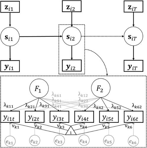
Measurement part

The measurement part shows how the state memberships define the responses. Thereby, it is important to note that the responses at time-point $t,$${\mathbf{y}}_{it},$ depend only on the latent state $k(k=1,\dots ,K)$ at that time-point and the responses are thus independent of the responses at other time-points given that state (“independence assumption”), which is also illustrated in Figure 1. In LMFA, the factor model depends on the state membership of subject $i$ at time-point $t$ (denoted by $s_{\mathit{itk}}=1$) as follows: (1) $$\left[{\mathbf{y}}_{it}\right|s_{\mathit{itk}}=1]= {\mathbf{\nu }}_k+{\mathbf{\Lambda }}_k {\mathbf{f}}_{\mathit{itk}}+ {\mathbf{e}}_{\mathit{itk}}.$$(1)

In this equation, ${\mathbf{\Lambda }}_k$ is the state-specific $J \times F_k$ loading matrix (where $F_k$ is the state-specific number of factors); ${\mathbf{f}}_{\mathit{itk}} \sim \mathit{MVN}(\mathbf{0},{\mathbf{\Psi }}_k)$ is the subject-specific $F_k\times 1$ vector of factor scores at time-point $t$ (where ${\mathbf{\Psi }}_k$ is the state-specific factor covariance matrix); ${\mathbf{\nu }}_k$ is the state-specific $J \times 1$ intercept vector; and ${\mathbf{e}}_{\mathit{itk}} \sim \mathit{MVN}(\mathbf{0},{\mathbf{D}}_k)$ the subject-specific $J \times 1$ vector of residuals at time-point $t$ (with ${\mathbf{D}}_k$ containing the unique variances $d_{kj}$ on the diagonal and zeros on the off-diagonal). Thus, the state-specific response densities, $p\left({\mathbf{y}}_{it}\right| s_{\mathit{itk}}=1),$ are defined by state-specific multivariate normal distributions with means ${\mathbf{\nu }}_k$ and covariance matrices ${\mathbf{\Sigma }}_k={\mathbf{\Lambda }}_k{\mathbf{\Lambda }}_k^{\prime }+{\mathbf{D}}_k.$ To obtain the state-specific factor models, LMFA employs exploratory factor analysis within the states in order to retain maximal flexibility regarding the differences in MMs that can be traced. In contrast to confirmatory factor analysis, exploratory factor analysis puts no a priori constraints on the factor loadings. However, if desired, confirmatory factor analysis can also be used.

From Eq. (1)(1) $$\left[{\mathbf{y}}_{it}\right|s_{\mathit{itk}}=1]= {\mathbf{\nu }}_k+{\mathbf{\Lambda }}_k {\mathbf{f}}_{\mathit{itk}}+ {\mathbf{e}}_{\mathit{itk}}.$$(1) we can see that the state-specific MMs may differ with regard to their loadings ${\mathbf{\Lambda }}_k,$ intercepts ${\mathbf{\nu }}_k,$ unique variances ${\mathbf{D}}_k,$ and factor (co)variances ${\mathbf{\Psi }}_k,$ implying that LMFA explores all levels of measurement non-invariance, that is, configural invariance (invariant number of factors and pattern of zero loadings), weak factorial invariance (invariant loading values), strong factorial invariance (invariant intercepts), and strict factorial invariance (invariant unique variances) (for more details see, e.g., Meredith, 1993). For identification purposes, the factor variances are equal to one in all the states and rotational freedom is dealt with by means of criteria to optimize simple structure and/or the between-state agreement of the factor loadings (e.g., Clarkson & Jennrich, 1988; De Roover & Vermunt, 2019; Kiers, 1997).

It is important to note that restricting the factors to have a mean of zero and a variance of one has the consequence that changes in factor means and variances may be captured as changes in the intercepts and loadings (i.e., if an additional state is selected for such a change). Therefore, when all intercepts that pertain to the same factor are higher or lower in one state compared to the other, it might be a sign that the factor means rather than separate intercepts differ across these states. Similarly, if all loadings of the same factor are likewise larger or smaller (i.e., the scaling is affected), it might be a sign that factor variances rather than the separate loadings differ across states. However, when the number of factors differs across states, it does not make sense to disentangle loading differences from factor-variance differences and, as long as weak invariance is violated, it does not make sense to disentangle intercept differences from factor-mean differences. In contrast, if the loadings and intercepts are (at least partially) invariant⁵, one could go ahead with an adjusted LMFA—that means, with equality restrictions on the MM parameters and including state-specific factor variances and means—and capture discrete changes in factor variances and means over time, as was already mentioned in the Introduction.

Furthermore, LMFA currently assumes that factors have no auto- and cross-lagged correlations at consecutive time-points. By means of a dynamic factor analysis, it would be possible to incorporate such autocorrelations, but factor rotation would be more intricate as auto- and cross-lagged relations have to be rotated toward a priori specified target matrices (Browne, 2001; Zhang, 2006). This would require a priori hypotheses about MM changes that are often not present or incomplete and that are thus undesired in exploratory studies. In addition, one would require more measurement occasions per subject (Ram et al., 2012), which is often unfeasible. In order to investigate whether ignoring autocorrelations in the data would pose problems for LMFA, Vogelsmeier, Vermunt, van Roekel, and De Roover (2019) conducted a simulation study using the FIML estimation and showed that the state and parameter recovery of the MMs were largely unaffected. Note, however, that ignoring dependency in the data leads to an underestimation of standard errors (SEs) of the MM parameters. This is only relevant when using hypothesis tests to trace significant differences in the MMs across states, which is possible by means of Wald tests using De Roover and Vermunt (2019)’s recently developed “multigroup factor rotation”.⁶ One would then have to correct for the dependency in the data (e.g., with the “primary sampling unit” identifier in LG; Vermunt & Magidson, 2016). Otherwise, invariance of parameters would be rejected too easily. However, the hypothesis tests are outside the scope of this paper.

Structural part

A latent Markov model generalizes a latent class model—the statistical method to identify subgroups with a similar set of indicator values—because subjects can transition between classes in a latent Markov model, while subjects remain in the same classes in a latent class model. The classes in a latent Markov model are therefore referred to as “states”. For an extensive description of latent Markov models, see, for example, Bartolucci, Farcomeni, et al. (2015) and Zucchini et al. (2016). In brief, transitions between the states are captured by a latent “Markov chain” defined by the probabilities to start in a state $k$ at time-point $t=1$ (“initial state probabilities”) and the probability of being in a state $k$ at time-point $t>1$ conditional on the occupied state $l (l=1,\dots ,K)$ at $t-1$ (“transition probabilities”). Note that, according to the first-order Markov assumption, the probability of being in a certain state $k$ at time-point $t$ depends only on the state at $t-1.$ The initial state probabilities are given by the $K\times 1$ probability vector $\mathbf{\pi },$ which contains the elements ${\pi }_k=p\left(s_{1k}=1\right)$ with $s_{tk}$ referring to the state membership $k$ at time-point $t$ (e.g., if a subject is in state 1 at time-point 1, then $s_{11}=1$ and $s_{12}=\cdots =s_{1K}=0$). These binary variables are in turn collected in the membership vectors ${\mathbf{s}}_{it}=\left(s_{it1},\dots ,s_{\mathit{itK}}\right)\prime ,$ for $t=1,\dots ,T,$ which are in turn collected in the $K\times T$ state membership matrix $\mathbf{S}=\left({\mathbf{s}}_{i1},{\mathbf{s}}_{i2},\dots ,{\mathbf{s}}_{iT}\right).$ The transition probabilities are collected in the $K\times K$ matrix $\mathbf{P},$ which contains the elements $p_{\mathit{lk}}=p(s_{tk}=1|s_{t-1,l}=1).$ Note that the rows indicate the state that a person comes from and the columns determine the state where the person transitions to. Hence, the diagonal elements represent the probabilities to stay in a state and the off-diagonal elements the probabilities to transition to another state. Therefore, diagonal values close or equal to 1 indicate stable state memberships and, thus, within-person invariance. It applies that the sum of the initial state probabilities, ${\sum }_{k=1}^K{\pi }_k,$ and the row sums of the transition probabilities, ${\sum }_{k=1}^K{p}_{\mathit{lk}},$ equal 1.

In the discrete-time latent Markov model, the time-intervals between observations are assumed to be equal. This assumption is often not tenable in empirical data. For instance, the questionnaires in ESM are usually send out at random moments and participants may skip certain measurement occasions, which automatically increases the distance between two subsequent observations. To accommodate such data, a continuous-time latent Markov model can be employed, which allows for differing intervals across time-points and subjects by considering the length of time spent in a state, $\delta .$ In the following, we provide a brief summary. The interested reader is referred to Böckenholt (2005) and Jackson and Sharples (2002) for general information about continuous-time latent Markov model and to Vogelsmeier, Vermunt, Böing-Messing, and De Roover (2019) for more specific information on continuous-time-LMFA. In brief, transitioning from the origin state $l$ to destination state$k$ is defined by the “intensities” (or rates) $q_{lk}$(collected in the $K\times K$ intensity matrix $\mathbf{Q}$) that replace the transition probabilities $p_{lk}$ and can be seen as probabilities to transition between states per very small time unit: (2) $$q_{lk}=\underset{\delta \to 0}{\mathit{lim}}\frac{p(s_{tk}=1|s_{t-\delta ,l}=1)}{\delta },$$(2) for all $k\ne l$ (thus, for the off-diagonal elements in the intensity matrix $\mathbf{Q}$). The diagonal elements are equal to the negative row sums (i.e., $-{\sum }_{k\ne l}{q}_{lk};$ Cox & Miller, 1965). The transition probabilities for any interval of interest can be computed by taking the matrix exponential of $\mathbf{Q}\times \delta .$ Note that larger time-intervals $\delta$ increase the probability to transition to a different state. In turn, $\mathbf{Q}$ can be obtained by taking the matrix logarithm of $\mathbf{P}.$⁷

In the following, we expand the structural part by including $U$ subject and possibly time-point specific covariates $z_{\mathit{itu}}$ (collected in the $U\times 1$ vectors ${\mathbf{z}}_{it}$) such that they affect the initial and transition probabilities.⁸ Note that the measurement part is assumed to be not (directly) affected by the covariates, which can also be seen in Figure 1. Also note that the parameters of the structural part are typically modeled using a logit model (for initial and transition probabilities) or via a log-linear model (for transition intensities) in order to prevent parameter space restrictions, which is also what LG does. The covariates enter the model through these parameterizations. For the initial state probabilities, we use the parameterization (3) $$\log \frac{p(s_{i1k}=1|{\mathbf{z}}_{i1})}{{p(s}_{i11}=1\left|{\mathbf{z}}_{i1}\right)}={\beta }_{0k}+{\mathbf{\beta }}_k^{\prime }{\mathbf{z}}_{it=1},$$(3) with $k=2,\dots ,K$ and $k=1$ as the reference category. The coefficients ${\beta }_{0k}$ are the initial state intercepts and ${\mathbf{\beta }}_k^{\prime }=({\beta }_{k,z_{i11}},\dots ,{\beta }_{k,z_{i1U}})\prime$ are the initial state slopes, which quantify the effect of the covariates on the initial state memberships. In discrete-time-LMFA, the multinomial logistic model for the transition probabilities is (4) $$\log \frac{p(s_{\mathit{itk}}=1|{s_{it-1,l}=1,\mathbf{z}}_{it})}{{p(s}_{\mathit{itl}}=1|s_{it-1,l}=1,{\mathbf{z}}_{it})}={\gamma }_{0lk}+{\mathbf{\gamma }}_{lk}^{\prime }{\mathbf{z}}_{it}$$(4) with $k\ne l.$ Thus, the logit is modeled by comparing the transition from state $l$ to state $k$ with the probability of staying in state $l.$ The coefficients ${\gamma }_{0lk}$ are the transition intercepts and ${\mathbf{\gamma }}_{lk}^{\prime }=({\gamma }_{lk,z_{\mathit{itu}}},\dots ,{\gamma }_{lk,z_{\mathit{itU}}})\prime$ are the transition slopes, which quantify the effect of the covariates on transitioning to another state. In continuous-time-LMFA, we use a log-linear model for the transition intensities (for $k\ne l$): (5) $$\log q_{\mathit{lk}}={\gamma }_{0lk}+{\mathbf{\gamma }}_{lk}^{\prime }{\mathbf{z}}_{it}.$$(5)

Finally, the joint distribution of observations and states, given the covariates, is (6) $$p\left({\mathbf{Y}}_i,{\mathbf{S}}_i|{\mathbf{Z}}_i\right)=p\left({\mathbf{y}}_{i1},\dots ,{\mathbf{y}}_{iT, }{\mathbf{s}}_{i1}, \dots , {\mathbf{s}}_{iT}|{\mathbf{z}}_{i1},\dots ,{\mathbf{z}}_{iT}\right)=p\left({\mathbf{s}}_{i1}\right|{\mathbf{z}}_{i1})\prod _{t=2}^T{p}_{{\delta }_{ti}}\left({\mathbf{s}}_{it}\right|{{\mathbf{s}}_{it-1},\mathbf{z}}_{it})\prod _{t=1}^{T}p\left({\mathbf{y}}_{it}\right|{\mathbf{s}}_{it}).$$(6)

Note that the ${\delta }_{ti}$ in $p_{{\delta }_{ti}}\left({\mathbf{s}}_{it}\right|{{\mathbf{s}}_{it-1},\mathbf{z}}_{it})$ refers to the transition probabilities’ dependency on the subject- and time-point-specific time-interval in continuous-time-LMFA. The term reduces to $p\left({\mathbf{s}}_{it}\right|{{\mathbf{s}}_{it-1},\mathbf{z}}_{it})$ in discrete-time-LMFA.

FIML estimation of latent Markov factor analysis (FIML-LMFA)

In order to obtain the maximum likelihood (ML) parameter estimates with the FIML estimation, the following loglikelihood function has to be maximized: (7) $${\log L}_{\mathit{FIML}}=\sum _{i=1}^I\log \left(\sum _{{\mathbf{s}}_{i1}}\dots \sum _{{\mathbf{s}}_{iT}}p\left({\mathbf{Y}}_i,{\mathbf{S}}_i|{\mathbf{Z}}_i\right)\right),$$(7) with $p\left({\mathbf{Y}}_i,{\mathbf{S}}_i|{\mathbf{Z}}_i\right)$ as given in Eq. (6)(6) $$p\left({\mathbf{Y}}_i,{\mathbf{S}}_i|{\mathbf{Z}}_i\right)=p\left({\mathbf{y}}_{i1},\dots ,{\mathbf{y}}_{iT, }{\mathbf{s}}_{i1}, \dots , {\mathbf{s}}_{iT}|{\mathbf{z}}_{i1},\dots ,{\mathbf{z}}_{iT}\right)=p\left({\mathbf{s}}_{i1}\right|{\mathbf{z}}_{i1})\prod _{t=2}^T{p}_{{\delta }_{ti}}\left({\mathbf{s}}_{it}\right|{{\mathbf{s}}_{it-1},\mathbf{z}}_{it})\prod _{t=1}^{T}p\left({\mathbf{y}}_{it}\right|{\mathbf{s}}_{it}).$$(6) . The ML estimates can be obtained by means of the forward-backward algorithm (Baum et al., 1970), which is an efficient version of the expectation maximization (EM; Dempster et al., 1977) algorithm and is also utilized by LG to find the ML solution. Within the maximization-step, a Fisher algorithm is used to update the state-specific covariance matrices defined by the factor models (Jennrich & Sampson, 1976) and, in case of continuous-time-LMFA, also to update the log-transition intensities. For a summary of the algorithms (including information about the convergence criteria and the utilized multistart procedure) see Vogelsmeier, Vermunt, van Roekel, and De Roover (2019) for discrete-time-LMFA and Vogelsmeier, Vermunt, Böing-Messing, et al. (2019) for continuous-time-LMFA.

It is important to note that we assume the number of states ($K$) and factors per state ($F_k)$ to be known when estimating the models. However, in real data, the best model in terms of the number of states and factors has to be evaluated. The Bayesian information criterion (BIC) performs well in selecting the best model in FIML-LMFA although the final decision regarding the optimal model should also take interpretability into account (Vogelsmeier, Vermunt, van Roekel, & De Roover, 2019). When also including covariates, every model under comparison (i.e., with all possible combinations of $K$ and $F_k$) has to be re-estimated every time a covariate is added or removed from the model because, using FIML estimation, the best model may change depending on the included covariates. For instance, when researchers want to obtain the best subset of $U=3$ covariate candidates, they would have to estimate $2^U=8$ times the number of models that is already under comparison. When all models are estimated, one may use the BIC and interpretability to choose the final model. Thus, the model selection quickly becomes overwhelming and even unfeasible when exploring relations between state memberships and many covariates.

Three-step estimation of latent Markov factor analysis (3S-LMFA)

In contrast to FIML-LMFA, 3S-LMFA decomposes the maximization problem for estimating the MMs and the SM into smaller parts. First, the state-specific MMs are estimated (step 1). Second, the observations are assigned to the MMs (i.e., classified to the states) and “classification errors” are calculated (step 2). Finally, the SM is estimated using the state-assignments while correcting for the classification errors (step 3). In the following, we explain the three steps in detail.

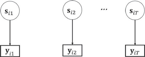
Step 1: Estimation of the state-specific measurement models

The first step as illustrated in Figure 2 involves estimating the state-specific MMs underlying the data by means of mixture factor analysis (McLachlan & Peel, 2000; McNicholas, 2016). The structural part (including the covariates) can be validly ignored because, in LMFA, the observations at a given time-point t, ${\mathbf{y}}_{\mathit{it}},$ are assumed to be conditionally independent of the state at time-point $t-1,$ $s_{\mathit{itl}}=1,$ and the covariates at time-point $t,$ ${\mathbf{z}}_{\mathit{it}},$ given the state membership at time-point $t,$ $s_{\mathit{itk}}=1$ (see Figure 1). For the estimation, all repeated observations are treated as “independent” such that respectively, say, 100 observations for each of 100 subjects results in 10,000 independent observations. The model parameters of interest are the state proportions $p\left(s_{\mathit{itk}}=1\right)$ and the state-specific response probabilities $p\left({\mathbf{y}}_{\mathit{itk}}|s_{\mathit{itk}}=1\right) =\mathit{MVN}({\mathbf{y}}_{\mathit{itk}}|{\mathbf{\nu }}_k,{\mathbf{\Lambda }}_k{\mathbf{\Lambda }}_k+{\mathbf{D}}_k).$ The mixture factor analysis model is therefore (8) $$p\left({\mathbf{y}}_{\mathit{it}}\right)=\sum _{k=1}^{K}p\left(s_{\mathit{itk}}=1\right)p\left({\mathbf{y}}_{\mathit{itk}}|s_{\mathit{itk}}=1\right)$$(8) and the loglikelihood function is (9) $${\log L}_{\mathit{STEP}1}=\sum _{i=1}^I\sum _{t=1}^T\log p\left({\mathbf{y}}_{\mathit{it}}\right).$$(9)

Figure 2. Step 1: Estimating the measurement model by performing mixture factor analysis. Note that the dependence of the observations is disregarded, which is indicated by the missing arrows between the latent states.

In LG, the posterior state probabilities and the state-specific factor models are estimated with an EM algorithm with Fisher scoring (Lee & Jennrich, 1979) in the maximization-step.⁹

As already discussed in the introduction, in this step, one also selects the optimal number of states $K$ and factors per state $F_k$ without having to be concerned about the covariates. Although the BIC is also a commonly used model selection criterion for mixture factor analysis (McNicholas, 2016), the CHull (Ceulemans & Kiers, 2006) method—which also balances model complexity and fit—proved to outperform the BIC in mixture factor analysis, especially when considering the three best models (Bulteel et al., 2013). Based on their results, we suggest to use the CHull method, potentially combined with the BIC, to select the three best models and compare them in terms of interpretability.

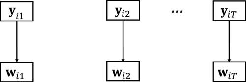
Step 2: Classification of observations and calculation of the classification error

Once the state-specific MMs have been estimated, in the second step, we allocate each observation to one of the $K$ states (see Figure 3). Therefore, we create a new variable ${\mathbf{w}}_{it}=\left(w_{it1},\dots ,w_{\mathit{itK}}\right)\prime ,$ that, similar to ${\mathbf{s}}_{it},$ represents the assignments of the observations to the estimated MMs from step 1. These predicted state memberships are based on the estimated posterior state probabilities $p\left(s_{\mathit{itk}}=1|{\mathbf{Y}}_{\mathit{it}}\right)$ from step 1, which can be expressed using Bayes’ theorem as (10) $$p\left(s_{\mathit{itk}}=1|{\mathbf{y}}_{\mathit{it}}\right)=\frac{p\left(s_{\mathit{itk}}=1\right)p\left({\mathbf{y}}_{\mathit{it}}|s_{\mathit{itk}}=1\right)}{p\left({\mathbf{y}}_{\mathit{it}}\right)}=\frac{p\left(s_{\mathit{itk}}=1\right)p\left({\mathbf{y}}_{\mathit{it}}|s_{\mathit{itk}}=1\right)}{\sum _{k\prime =1}^{K}p\left(s_{\mathit{itk}\prime }=1\right)p\left({\mathbf{y}}_{\mathit{it}}|s_{\mathit{itk}\prime }=1\right)}.$$(10)

Figure 3. Step 2: Assigning states and calculating the classification error.

Thus, all observations ${\mathbf{y}}_{\mathit{it}}$ belong to each of the $K$ states with a certain probability $p\left(s_{\mathit{itk}}=1|{\mathbf{y}}_{\mathit{it}}\right).$ There are two common rules¹⁰ on how to proceed with these posterior state probabilities with regard to the final state assignments. First, “proportional assignment” assigns a state according to the posterior probabilities such that $p\left(w_{\mathit{itk}}=1|{\mathbf{y}}_{\mathit{it}}\right)=p\left(s_{\mathit{itk}}=1|{\mathbf{y}}_{\mathit{it}}\right),$ which leads to a “soft” partitioning. Second, “modal assignment” allocates the weight $p\left(w_{\mathit{itk}}=1|{\mathbf{y}}_{\mathit{it}}\right)=1$ for the state k with the largest posterior state probability in ${\mathbf{s}}_{it}$ and a zero weight for all others states. Note that we will focus on modal assignment because proportional assignment is unfeasible with a large number of time-points per subject, which would involve separate weights for all $K^T$ possible combinations of states in case of classification uncertainty (Di Mari et al., 2016).

Regardless of the assignment rule, classification error is inherent to any assignment procedure because the largest posterior probability is usually not equal to 1. We have to account for this error because, if not accounted for, the error attenuates relationships between variables. On the one hand, this attenuation will lead to an underestimation of the relation among true states ${\mathbf{s}}_{it}$ at two consecutive time-points and thus, an overestimation of the transition probabilities away from a state (Vermunt et al., 1999). On the other hand, estimating the relationship between the estimated memberships ${\mathbf{w}}_{it}$ and covariates ${\mathbf{z}}_{it}$—instead of using the true states ${\mathbf{s}}_{it}$—causes underestimation of the covariate effects (Di Mari et al., 2016). Hence, a correction for attenuation of relationships due to classification error is necessary.

In order to calculate the classification error so that we can account for it in step 3, we have to obtain the probability of a certain state assignment $w_{\mathit{itm}}=1$ conditional on the true state $s_{\mathit{itk}}=1,$ $p\left(w_{\mathit{itm}}=1|s_{\mathit{itk}}=1\right),$ for all $k,m=1,\dots , K.$ These probabilities are collected in the $K\times K$ “classification error probability matrix”. They are computed as (11) $$p\left(w_{\mathit{itm}}=1|s_{\mathit{itk}}=1\right)=\frac{\int p\left(w_{\mathit{itm}}=1|{\mathbf{y}}_{\mathit{it}}\right)p\left({\mathbf{y}}_{\mathit{it}}\right)p\left(s_{\mathit{itk}}=1|{\mathbf{y}}_{\mathit{it}}\right)d{\mathbf{y}}_{\mathit{it}}}{p\left(s_{\mathit{itk}}=1\right)}.$$(11)

For the derivation, see the Appendix A.1.1. To solve this equation, $p\left({\mathbf{y}}_{\mathit{it}}\right)$ can be validly substituted by its empirical distribution (Di Mari et al., 2016; Vermunt, 2010), resulting in (12) $$p\left(w_{\mathit{itm}}=1|s_{\mathit{itk}}=1\right)=\frac{\frac{1}{I\times T}\sum _{i=1}^I\sum _{t=1}^T\hspace{0.17em}p\left(w_{\mathit{itm}}=1|{\mathbf{y}}_{\mathit{it}}\right)p\left(s_{\mathit{itk}}=1|{\mathbf{y}}_{\mathit{it}}\right)}{p\left(s_{\mathit{itk}}=1\right)}.$$(12)

Note that another option to solve the integral would be to use Monte Carlo simulation. The larger the probabilities for $m=k$ (corresponding to the diagonal elements of the classification error probability matrix), the better the classification and thus, the smaller the classification error. Note that classification error is strongly related to separation between the states (i.e., how well the latent states are predicted by $\mathbf{Y}=\left({\mathbf{Y}}_1^{\prime },{\mathbf{Y}}_2^{\prime },\dots ,{\mathbf{Y}}_I^{\prime }\right);$ Bakk et al., 2013; Vermunt, 2010). To qualify the separation in any LC analysis, an entropy-based (pseudo) R-squared measure, $R_{\mathit{entropy}}^2,$ is commonly used (Lukočienė et al., 2010; Vermunt & Magidson, 2016; Wedel & Kamakura, 1998). The $R_{\mathit{entropy}}^2$ value defines the relative improvement of predicting the state membership when using the observations ${\mathbf{y}}_{\mathit{it}}$ compared to predicting the state membership without ${\mathbf{y}}_{\mathit{it}}.$ Values range from zero (prediction is no better than chance) to one (perfect prediction). State separation (and hence classification error) depends on various factors. For example, it increases with a lower number of states, higher factor overdetermination (which is higher in case of less factors, more variables, or lower unique variances), and lower between-state similarity (determined by larger differences in the state-specific MMs). The $R_{\mathit{entropy}}^2$ values for the different settings in our simulation study will be reported below in Section “Design and Procedure”.

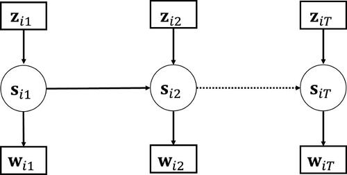
Step 3: Estimation of the structural model

In the final step, we estimate the SM (i.e., the Markov model with covariates), which is illustrated in Figure 4. The key to correct for the classification error obtained in step 2 is to show the relationship between the estimated state memberships conditional on the covariates, $p({\mathbf{W}}_i|{\mathbf{Z}}_i),$ and the true state memberships conditional on the covariates, $p({\mathbf{S}}_i|{\mathbf{Z}}_i),$ where ${\mathbf{W}}_i=({\mathbf{w}}_{i1},{\mathbf{w}}_{i2},\dots ,{\mathbf{w}}_{iT}),$ ${\mathbf{Z}}_i=({\mathbf{z}}_{i1},{\mathbf{z}}_{i2},\dots ,{\mathbf{z}}_{\mathit{iT}})$ and ${\mathbf{S}}_i=({\mathbf{s}}_{i1},{\mathbf{s}}_{i2},\dots ,{\mathbf{s}}_{iT})$ (Di Mari et al., 2016). Therefore, we consider the joint probability $p\left({\mathbf{W}}_i,{\mathbf{Y}}_i,{\mathbf{S}}_i,{\mathbf{Z}}_i\right)$ and solve for $p({\mathbf{W}}_i|{\mathbf{Z}}_i)$ (see Appendix A.1.2), which results in (13) $$p({\mathbf{W}}_i|{\mathbf{Z}}_i)=\sum _{{\mathbf{s}}_{i1}}\cdots \sum _{{\mathbf{s}}_{iT}}p({\mathbf{s}}_{i1}|{\mathbf{z}}_{i1})\prod _{t=2}^{T}p\left({\mathbf{s}}_{it}\right|{{\mathbf{s}}_{it-1},\mathbf{z}}_{it})\prod _{t=1}^{T}p({\mathbf{w}}_{it}|{\mathbf{s}}_{it}).$$(13)

Figure 4. Step 3: Estimating the structural model by means of a latent Markov model with single indicators ${\mathbf{w}}_{it}.$

It can be seen that Eq. (13)(13) $$p({\mathbf{W}}_i|{\mathbf{Z}}_i)=\sum _{{\mathbf{s}}_{i1}}\cdots \sum _{{\mathbf{s}}_{iT}}p({\mathbf{s}}_{i1}|{\mathbf{z}}_{i1})\prod _{t=2}^{T}p\left({\mathbf{s}}_{it}\right|{{\mathbf{s}}_{it-1},\mathbf{z}}_{it})\prod _{t=1}^{T}p({\mathbf{w}}_{it}|{\mathbf{s}}_{it}).$$(13) resembles the FIML-LMFA model from Eq. (6)(6) $$p\left({\mathbf{Y}}_i,{\mathbf{S}}_i|{\mathbf{Z}}_i\right)=p\left({\mathbf{y}}_{i1},\dots ,{\mathbf{y}}_{iT, }{\mathbf{s}}_{i1}, \dots , {\mathbf{s}}_{iT}|{\mathbf{z}}_{i1},\dots ,{\mathbf{z}}_{iT}\right)=p\left({\mathbf{s}}_{i1}\right|{\mathbf{z}}_{i1})\prod _{t=2}^T{p}_{{\delta }_{ti}}\left({\mathbf{s}}_{it}\right|{{\mathbf{s}}_{it-1},\mathbf{z}}_{it})\prod _{t=1}^{T}p\left({\mathbf{y}}_{it}\right|{\mathbf{s}}_{it}).$$(6) , marginalized over ${\mathbf{S}}_i$ and with different response probabilities. It is in fact a latent Markov model with the state assignments from ${\mathbf{W}}_i$ as single indicators with $K$ categories replacing the observed item responses ${\mathbf{Y}}_i.$ This demonstrates that ${\mathbf{Y}}_i$ is no longer needed in step 3 if we have the classification error probabilities $p\left({\mathbf{w}}_{it}|{\mathbf{s}}_{it}\right).$ The response probabilities are fixed to the classification error probabilities and thus do not have to be estimated. Hence, the focus of the latent Markov model changes. Instead of accounting for unobserved heterogeneity of the MMs (as in FIML-LMFA), the latent Markov model accounts for error in the estimated state assignments ${\mathbf{W}}_i.$

In order to estimate the SM, the following loglikelihood function has to be maximized: (14) $${\log L}_{\mathit{STEP}3}=\sum _{i=1}^I\log \left(p\left({\mathbf{W}}_i\right|{\mathbf{Z}}_i)\right).$$(14)

The estimation, just as in the regular FIML-LMFA, is done by means of the forward-backward algorithm.¹¹ However, the classification error probabilities are utilized as fixed response probabilities, such that only the (covariate-specific) transition and initial-state probabilities need to be estimated. Note that the state-assignments ${\mathbf{W}}_i$ are treated as the manifest (i.e., observed) indicators (that contain error) of the “true” (error-free) latent states ${\mathbf{S}}_i,$ which are inferred through the forward-backward algorithm and used to determine the parameters of the SM. Differences between ${\mathbf{W}}_i$ and ${\mathbf{S}}_i$ become less likely for well-separated states with small classification error.

Finally, as already discussed in the Introduction, in the third step, one evaluates which covariates significantly relate to the transition and/or initial state probabilities. Instead of selecting the best subset of covariates by means of an information criterion as in the FIML approach, one may start with a model including all covariate candidates or none of them and use Wald (or likelihood ratio) tests to decide which covariates can be removed from or added to the model one by one (e.g., using forward or backward elimination). Note that, as in any statistical model, there are advantages and disadvantages with regard to such data-driven covariate selection procedures (for a review, see Heinze et al., 2018). When in doubt, one may conduct sensitivity analyses comparing the results from different approaches. When having strong a priori hypotheses about covariates, one may also consider a more theory-driven approach.

Simulation study

Problem

The aim of the simulation study was to evaluate the performance of 3S-LMFA and to see if it approaches the performance of FIML-LMFA. The specific targeted measures were recovery of the states (i.e., the classification), the MM parameters, and the parameters and SEs of the SM consisting of the Markov model with covariate effects. First, parameter and state recovery have previously been shown to be positively influenced by an increasing amount of information (in terms of sample size) and by higher state-separation (i.e., a better distinction between the states; Bakk et al., 2013; Di Mari et al., 2016; Vermunt, 2010). The more information is available and the more separable the states are, the more accurate the mixture factor analysis can estimate the MM parameters in step 1 and the more accurate the estimation of the SM in step 3.

Second, SEs are possibly slightly underestimated because the error probabilities $p\left(w_{\mathit{itm}}=1|s_{\mathit{itk}}=1\right)$ are assumed to be known in step 3 although they are actually estimated parameters of the mixture factor analysis in step 1. When the SEs are underestimated, the Wald statistic to test covariate effects would lead to wrong conclusions regarding the statistical significance of covariates. If this underestimation is present, it will likely vanish with large state separation and amount of information (Di Mari et al., 2016; Vermunt, 2010). In the simulation study, we evaluate whether underestimation is present and from what point on state separation and amount of information are sufficient to obtain trustworthy SE values.

Third, the $R_{\mathit{entropy}}^2$ and thus the state separation is higher for FIML-LMFA than for the initial state separation in the first step of 3S-LMFA because the former has additional information from the SM (i.e., the covariates and the states occupied at adjacent time-points) while the latter has information only from the MMs in step 1. Therefore, the recovery of the state memberships is expected to be better for FIML-LMFA. We expect this difference in recovery to decrease when the state memberships are updated in step 3 (i.e., when the SM is also included). However, the degree to which the state-membership recovery in 3S-LMFA approaches the recovery in FIML has to be demonstrated in the simulation study.

Note that the evaluation of the model selection procedures in step 1 (i.e., finding the best number of states, $K,$ and factors per state, $F_k$ by means of the BIC and the CHull) and step 3 (i.e., selecting the correct covariates by means of Wald tests, e.g., with backward elimination) is beyond the scope of this paper and will be used only in the application. As described in Section “Step 1: Estimation of the State-Specific Measurement Models”, the BIC and the CHull have already been extensively evaluated for mixture factor analysis. Furthermore, when the simulation study shows that the covariate parameters and their SEs are estimated correctly, we believe that the Wald tests will also correctly identify the significant covariates. However, in Section “Discussion”, we will discuss the possibility of inaccurate model selection under the violation of the conditional independence assumption.

We manipulated the two key factors: (1) state-separation¹² (this includes (a) between-state loading differences and (b) intercept differences) and (2) amount of information (this includes (c) number of subjects and (d) number of participation days per subject). Note that, for selected conditions, we also investigated whether 3S-LMFA might be more affected by ignoring autocorrelation than FIML-LMFA (see Appendix A.2) and whether varying the strength of the covariate effects and the distribution of the covariates across observations or subjects impacted the estimation procedures differently (see Appendix A.3), which was not the case.

Design and procedure

The conditions were the following: $$\begin{array}{cc}\text{State‐separation}& \{\begin{array}{l}\text{a}\text{.\hspace{0.17em}\hspace{0.17em}Between}‐\text{state\hspace{0.17em}\hspace{0.17em}loading\hspace{0.17em}\hspace{0.17em}differences\hspace{0.17em}\hspace{0.17em}at\hspace{0.17em}\hspace{0.17em}two\hspace{0.17em}\hspace{0.17em}levels}:\\ \text{medium\hspace{0.17em}\hspace{0.17em}loading\hspace{0.17em}\hspace{0.17em}differences},\text{\hspace{0.17em}\hspace{0.17em}low\hspace{0.17em}\hspace{0.17em}loading\hspace{0.17em}\hspace{0.17em}differences};\\ \text{b}\text{.\hspace{0.17em}\hspace{0.17em}Between}‐\text{state\hspace{0.17em}\hspace{0.17em}intercept\hspace{0.17em}\hspace{0.17em}differences\hspace{0.17em}\hspace{0.17em}at\hspace{0.17em}\hspace{0.17em}two\hspace{0.17em}\hspace{0.17em}levels}:\\ \text{no\hspace{0.17em}\hspace{0.17em}intercept\hspace{0.17em}\hspace{0.17em}differences},\text{\hspace{0.17em}\hspace{0.17em}low\hspace{0.17em}\hspace{0.17em}intercept\hspace{0.17em}\hspace{0.17em}differences};\end{array}\end{array}\begin{array}{cc}\text{Amount\hspace{0.17em}\hspace{0.17em}of\hspace{0.17em}\hspace{0.17em}information}& \{\begin{array}{l}\text{c}\text{.\hspace{0.17em}\hspace{0.17em}Number\hspace{0.17em}\hspace{0.17em}of\hspace{0.17em}\hspace{0.17em}Subjects}N\text{at\hspace{0.17em}\hspace{0.17em}four\hspace{0.17em}\hspace{0.17em}levels}:\text{\hspace{0.17em}\hspace{0.17em}3}0,\text{\hspace{0.17em}\hspace{0.17em}5}0,\text{\hspace{0.17em}\hspace{0.17em}7}0,\text{\hspace{0.17em}\hspace{0.17em}9}0;\\ \text{d}\text{.\hspace{0.17em}\hspace{0.17em}Number\hspace{0.17em}\hspace{0.17em}of\hspace{0.17em}\hspace{0.17em}days}D\text{at\hspace{0.17em}\hspace{0.17em}two\hspace{0.17em}\hspace{0.17em}levels}:\text{\hspace{0.17em}\hspace{0.17em}7},\text{\hspace{0.17em}\hspace{0.17em}3}0;\end{array}\end{array}$$

This design resulted in $2\times 2\times 4\times 2=32$ conditions. For the population model, we used an ESM setup—with number of subjects, $N,$ days, $D,$ and observations per day, $T_{\mathit{day}}$—that is often found in practice (e.g., van Roekel et al., 2019; Van Roekel et al., 2017). Furthermore, we used unequal time-intervals that are typical for ESM studies and, therefore, employed continuous-time-LMFA. Thereby, the following values were used as constants: number of items $J=20,$ unique variances $e=.2,$ number of states $K=3,$ number of factors $F_k=F=2,$ and number of observations per day $T_{\mathit{day}}=9.$ The latter also determined the ESM sampling scheme (comparable to Vogelsmeier, Vermunt, Böing-Messing, et al., 2019): Imposing that a sampling day lasts from 9 am to 9 pm, both day and night intervals were on average 12 hours long. The $T_{\mathit{day}}=9$ measurement occasions during the day lead to intervals of 1.5 hours if the measurement-occasions were fixed. However, for random variations, we let observations deviate from these fixed time-points by means of a uniform distribution with a maximum of plus and minus 30 percent of the fixed 1.5 hour intervals. Thus, the deviations were drawn from $\mathit{Unif}(-0.3\times 1.5, 0.3\times 1.5).$

To determine the SM, the initial state parameters were chosen to lead to equal probabilities of starting in a state (${\beta }_{02}={\beta }_{03}=0$). The transition intercept parameters were specified to be realistic for a short unit interval of 1.5 hours with high probabilities to stay in a state.¹³ More specifically, the intercept parameters were ${\gamma }_{012}={\gamma }_{013}={\gamma }_{021}={\gamma }_{023}={\gamma }_{031}={\gamma }_{032}=-3.65$ which would correspond to the following transition probability matrix if no covariates were present: (15) $${\mathbf{P}}_{\mathrm{day}}=\left(\begin{array}{ccc}.950& .025& .025\\ .025& .950& .025\\ .025& .05& .950\end{array}\right).$$(15)

To alter the transition probabilities, we used one time-varying dichotomous covariate ($z_{it1}),$ which changed in value after 3 days for $D=7$ or after 15 days for $D=30,$ and one time-constant dichotomous covariate ($z_{it2}=z_{i2})$ that was randomly assigned to the subjects with equal probabilities. Both covariates had values equal to $-0.5$ or $0.5.$ A higher value for $z_{it1}$ lowered the probabilities of transitioning to and staying in state 1 and 3 while increasing the probabilities of transitioning to and staying in state 2. For instance, this time-varying covariate could represent an intervention that increased the probability to move to and stay in a “healthy state”. The corresponding slope parameters were ${\gamma }_{12,z_{it1}}={\gamma }_{32,z_{it1}}=1$ and ${\gamma }_{13,z_{it1}}={\gamma }_{21,z_{it1}}={\gamma }_{23,z_{it1}}={\gamma }_{31,z_{it1}}=-0.5.$ Furthermore, a higher value for $z_{i2}$ increased the probability to transition away from the origin state, leading to a less stable Markov chain. For instance, this stable variable could be a trait-like general stability in response behavior that influences all probabilities to transition away from the state at the previous time-point. The corresponding slope parameters were ${\gamma }_{12,Z_{it2}}={\gamma }_{13,z_{it2}}={\gamma }_{21,z_{it2}}={\gamma }_{23,z_{it2}}={\gamma }_{31,z_{it2}}={\gamma }_{32,z_{it2}}=0.5.$ The four resulting possibilities for the transition probability matrices were (16) $$\begin{array}{cc}{\mathbf{P}}_{z_{\mathit{it}1}=-.5, z_{\mathit{it}2}=-.5}=\left(\begin{array}{ccc}.963& .012& .025\\ .025& .950& .025\\ .025& .012& .963\end{array}\right),& {\mathbf{P}}_{z_{\mathit{it}1}=-.5, z_{\mathit{it}2}=.5}=\left(\begin{array}{ccc}.940& .019& .041\\ .041& .919& .041\\ .041& .019& .940\end{array}\right),\\ {\mathbf{P}}_{z_{\mathit{it}1 }= .5, z_{\mathit{it}2} = -.5}=\left(\begin{array}{ccc}.952& .032& .015\\ .015& .969& .015\\ .015& .032& .952\end{array}\right)& {\mathbf{P}}_{z_{\mathit{it}1} = .5, z_{\mathit{it}2} = .5}=\left(\begin{array}{ccc}.923& .052& .025\\ .025& .951& .025\\ .025& .052& .923\end{array}\right)\end{array},$$(16)

Note that the covariate effects appear to be rather small but they increase for larger intervals than the unit interval.

Regarding the state separation, we used the same conditions as in previous simulation studies evaluating LMFA (Vogelsmeier, Vermunt, Böing-Messing, et al., 2019; Vogelsmeier, Vermunt, van Roekel, & De Roover, 2019). More specifically, we generated data with state-specific MMs as defined in Eq. (1)(1) $$\left[{\mathbf{y}}_{it}\right|s_{\mathit{itk}}=1]= {\mathbf{\nu }}_k+{\mathbf{\Lambda }}_k {\mathbf{f}}_{\mathit{itk}}+ {\mathbf{e}}_{\mathit{itk}}.$$(1) , assuming orthogonal factors (i.e., ${\mathbf{f}}_{\mathit{itk}} \sim \mathit{MVN}(\mathbf{0},\mathbf{I})$). To induce the between-state loading differences, we started with a common base matrix in both states: (17) $${\mathbf{\Lambda }}_{\mathit{Base}}={\left(\begin{array}{cccccccccccccccccccc}1& 1& 1& 1& 1& 1& 1& 1& 1& 1& 0& 0& 0& 0& 0& 0& 0& 0& 0& 0\\ 0& 0& 0& 0& 0& 0& 0& 0& 0& 0& 1& 1& 1& 1& 1& 1& 1& 1& 1& 1\end{array}\right)}^{\mathbf{\text{'}}},$$(17) which shows a binary simple structure that is often found in empirical studies (e.g., consider a typical positive vs. negative affect structure that may also underlie the data in the motivating example described in Section “Motivating Example”). For the medium loading difference condition, respectively one loading was shifted from the first factor to the second and one from the second to the first (for different items across states). Through this manipulation, the overdeterminaton of the factors was not affected and thus equal across states. For example, the first two of three loading matrices were (18) $$\begin{array}{c}{\mathbf{\Lambda }}_1={\left(\begin{array}{cccccccccccccccccccc}{\mathrm{\lambda }}_1& 1& 1& 1& 1& 1& 1& 1& 1& 1& {\mathrm{\lambda }}_2& 0& 0& 0& 0& 0& 0& 0& 0& 0\\ {\mathrm{\lambda }}_2& 0& 0& 0& 0& 0& 0& 0& 0& 0& {\mathrm{\lambda }}_1& 1& 1& 1& 1& 1& 1& 1& 1& 1\end{array}\right)}^{\mathbf{\text{'}}}\\ {\mathbf{\Lambda }}_2={\left(\begin{array}{cccccccccccccccccccc}1& {\mathrm{\lambda }}_1& 1& 1& 1& 1& 1& 1& 1& 1& 0& {\mathrm{\lambda }}_2& 0& 0& 0& 0& 0& 0& 0& 0\\ 0& {\mathrm{\lambda }}_2& 0& 0& 0& 0& 0& 0& 0& 0& 1& {\mathrm{\lambda }}_1& 1& 1& 1& 1& 1& 1& 1& 1\end{array}\right)}^{\mathbf{\text{'}}}\end{array}$$(18) with ${\mathrm{\lambda }}_1=0$ and ${\mathrm{\lambda }}_2=1.$ Similarly, for the low between-state loading difference condition one cross-loading of $\sqrt{.5}$ was added to the first and second factor (for different items across states), which also lowered the primary loadings to $\sqrt{.5}.$ Specifically, in the example in Eq. (18)(18) $$\begin{array}{c}{\mathbf{\Lambda }}_1={\left(\begin{array}{cccccccccccccccccccc}{\mathrm{\lambda }}_1& 1& 1& 1& 1& 1& 1& 1& 1& 1& {\mathrm{\lambda }}_2& 0& 0& 0& 0& 0& 0& 0& 0& 0\\ {\mathrm{\lambda }}_2& 0& 0& 0& 0& 0& 0& 0& 0& 0& {\mathrm{\lambda }}_1& 1& 1& 1& 1& 1& 1& 1& 1& 1\end{array}\right)}^{\mathbf{\text{'}}}\\ {\mathbf{\Lambda }}_2={\left(\begin{array}{cccccccccccccccccccc}1& {\mathrm{\lambda }}_1& 1& 1& 1& 1& 1& 1& 1& 1& 0& {\mathrm{\lambda }}_2& 0& 0& 0& 0& 0& 0& 0& 0\\ 0& {\mathrm{\lambda }}_2& 0& 0& 0& 0& 0& 0& 0& 0& 1& {\mathrm{\lambda }}_1& 1& 1& 1& 1& 1& 1& 1& 1\end{array}\right)}^{\mathbf{\text{'}}}\end{array}$$(18) , the entries in ${\mathbf{\Lambda }}_1$ and ${\mathbf{\Lambda }}_2$ were ${\mathrm{\lambda }}_1=\sqrt{.5}$ and ${\mathrm{\lambda }}_2=\sqrt{.5}.$ Finally, row-wise rescaling of the loading matrices leads to a sum of squares of $1-e$ per row. The between-state loading matrix similarity was computed by means of the grand mean, ${\phi }_{\mathit{mean}},$ of Tucker’s (1951) congruence coefficient (i.e., ${\phi }_{xy}=\frac{x\prime y}{\sqrt{x\prime x}\sqrt{y\prime y}},$ with $x$ and $y$ referring to matrix columns) that was computed for each pair of factors (note that $\phi =1$ means proportionally identical factors). The ${\phi }_{\mathit{mean}}$ across all states and factors was respectively .80 and .94 for the medium and low loading difference condition$.$

For the intercepts, we used the following base vector with fixed values of 5: (19) $${\mathbf{\nu }}_{\mathit{Base}}={\left(\begin{array}{cccccccccccccccccccc}5& 5& 5& 5& 5& 5& 5& 5& 5& 5& 5& 5& 5& 5& 5& 5& 5& 5& 5& 5\end{array}\right)}^{\prime },$$(19) which was used as such in all states for the no intercept difference condition. To induce low intercept differences across states, we altered two intercepts to 5.5 (different items across the states). For example, for the first two states, the vectors were (20) $$\begin{array}{c}{\mathbf{\nu }}_1={\left(\begin{array}{cccccccccccccccccccc}5.5& 5.5& 5& 5& 5& 5& 5& 5& 5& 5& 5& 5& 5& 5& 5& 5& 5& 5& 5& 5\end{array}\right)}^{\mathrm{\text{'}}},\\ {\mathbf{\nu }}_2={\left(\begin{array}{cccccccccccccccccccc}5& 5& 5.5& 5.5& 5& 5& 5& 5& 5& 5& 5& 5& 5& 5& 5& 5& 5& 5& 5& 5\end{array}\right)}^{\mathrm{\text{'}}}.\end{array}$$(20) The combination of the between-state loading difference and intercept difference conditions lead to four different state-separation conditions. To quantify the general state-separation in both analyses based on the population values, we calculated the four $R_{\mathit{entropy}}^2$ values for step 1 of 3S-LMFA, where information is only obtained from the MM, and for FIML-LMFA, where information is retrieved from both the MM and the SM including the two covariates.¹⁴ For FIML-LMFA, starting from the smallest $R_{\mathit{entropy}}^2,$ the resulting values amounted to .90 for the low loading difference/no intercept difference condition, to .94 for the medium loading difference/no intercept difference condition, to .96 for the low loading difference/low intercept difference condition, and to .97 for the medium loading difference/low intercept difference condition. For the same conditions in the first step of 3S-LMFA, these values were respectively equal to .52, .65, .76, and .82. Thus, as expected, state-separation is initially lower in 3S-LMFA than in FIML-LMFA, showing the importance for 3S-LMFA to include the information from the SM in step 3.¹⁵

For each condition, we generated 100 datasets in R (R Core Team, 2020) according to the described population models and analyzed them in LG. Note that only one syntax file is required for FIML-LMFA but two files are necessary for 3S-LMFA. First, one syntax file is required to run step 1 and 2. Thereby, the posterior state assignments and the classification error probability matrix are saved and, subsequently, they are loaded in the second syntax file that is required for step 3.

Results

In the following, we evaluate the performance of 3S-LMFA and compare it to the results of FIML-LMFA based on the replications that converged in both steps of the 3S method as well as in the FIML method. Results that did not converge were re-estimated once and were excluded if convergence still failed. After re-estimation, 3180 out of 3200 datasets converged in 3S- and FIML-LMFA (all datasets converged in step 1 and step 3 of 3S-LMFA and 3180 in FIML-LMFA). Non-convergence in FIML was almost exclusively present for the smallest amount of information condition (i.e., $N=30$ and $D=7$) and was caused by reaching the maximum number of EM iterations without convergence. Furthermore, we re-estimated the replications of converged results that showed unrealistically large SEs due to boundary values for any of the estimated initial state and transition parameters (i.e., with an $\text{SE}>10$ such as 100, 400 or 1000) because including such cases would falsify the results. This was only the case for 56 datasets in the third step of 3S-LMFA, where re-estimation did not help. As a result, 3124 datasets were included in the performance analyses reported below.¹⁶

Goodness of state recovery

The recovery of the states was assessed by means of the Rand Index (RI) as well as the Adjusted Rand Index (ARI; Hubert & Arabie, 1985). Both indices evaluate the overlap between two sets of elements while being insensitive to permutations of element labels (in our case state labels). The indices in the RI range from 0 (no overlap between any of the pairs) to 1 (perfect overlap) and the ARI takes values from around 0 (overlap is not better than chance) to 1 (perfect overlap). As expected, the state-recovery was rather poor after the first step of 3S-LMFA because of the low $R_{\mathit{entropy}}^2$ values here ($RI=.83,$ ${SD}_{RI}=.06,$ $\mathit{ARI}=.61,$${SD}_{\mathit{ARI}}=.14$). However, the overall recovery in 3S-LMFA was excellent (Steinley, 2004; $RI=.94,$ ${SD}_{RI}=.03,$ $\mathit{ARI}=.87,$${SD}_{\mathit{ARI}}=.06$) and almost as high as in FIML-LMFA ($RI=.97,$ ${SD}_{RI}=.01,$ $\mathit{ARI}=.94,$${SD}_{\mathit{ARI}}=.03$). Moreover, only the state-separation influenced the state recovery in that larger separation increased recovery (Table 1), indicating that already the minimum sample size of $30 \left(N\right)\times 7 \left(D\right)\times 9 \left(T_{\mathit{day}}\right)=1890$ was sufficient to estimate $K=3$ states (and thus about 630 observations per state), which is largely in line with previous results showing that about 500 observations per state are sufficient for similar settings and that a higher amount of information in terms of sample size and observations per subject does not aid recovery once this threshold is reached (Vogelsmeier, Vermunt, van Roekel, & De Roover, 2019).

Table 1. Goodness of recovery for the states, loadings, intercepts and unique variances averaged across and conditional on the manipulated factors.

		Goodness of recovery
		States $(\mathit{ARI})$			States RI $(RI)$			Loadings $(\mathit{GOSL})$		Intercepts $({\mathit{MAD}}_{\mathit{int}})$		Unique variances $({\mathit{MAD}}_{\mathit{unique}})$
		Type of LMFA
Condition	Factors	3S-1	3S-3	FIML	3S-1	3S-3	FIML	3S	FIML	3S	FIML	3S	FIML
Between-State Loading Difference	low	.56	.85	.93	.80	.93	.97	1	1	.02	.02	.01	.01
	medium	.66	.89	.95	.85	.95	.98	1	1	.02	.02	.01	.01
Between-State Intercept Difference	no	.47	.81	.91	.77	.92	.96	1	1	.02	.02	.01	.01
	low	.74	.92	.97	.89	.97	.98	1	1	.02	.02	.01	.01
Number of Subjects N	30	.61	.87	.94	.83	.94	.97	1	1	.02	.02	.01	.01
	50	.61	.87	.94	.82	.94	.97	1	1	.02	.02	.01	.01
	70	.61	.87	.94	.83	.94	.97	1	1	.02	.02	.01	0
	90	.61	.87	.94	.83	.94	.97	1	1	.01	.01	0	0
Number of Participation Days D	7	.61	.86	.94	.83	.94	.97	1	1	.03	.02	.01	.01
	30	.61	.87	.94	.83	.94	.97	1	1	.01	.01	0	0
All Conditions
Average		.61	.87	.94	.83	.94	.97	1	1	.02	.02	.01	.01
SD		.14	.06	.03	.06	.03	.01	0	0	.01	.01	0	0

Note. LMFA = latent Markov factor analysis; 3S-1 = three-step step 1; 3S-3 = three-step step 3; FIML = full information maximum likelihood. The perfect loading recoveries result from the loading matrices that are highly similar across the states.

Goodness of MM parameter recovery

Goodness of loading recovery

We computed a goodness of state-loading recovery (GOSL) as the average Tucker congruence coefficient between the true and the estimated loading matrices: (21) $$\mathit{GOSL}= \frac{\sum _{k=1}^K\sum _{f=1}^F\phi ({\mathbf{\Lambda }}_k^f,{\widehat{\mathbf{\Lambda }}}_k^f)}{K\times F},$$(21) where ${\mathbf{\Lambda }}_k^f$ corresponds to the state- and factor-specific loadings. By using Procrustes rotation¹⁷ (Kiers, 1997) in order to rotate the estimated state-specific loading matrices ${\widehat{\mathbf{\Lambda }}}_k$ to the true ones ${\mathbf{\Lambda }}_k,$ we solved the label switching of the factor labels within the states. Furthermore, to handle the label switching of the states, we retained the state permutation that maximized the $\mathit{GOSL}$ value. Overall, the loading recovery was very good in 3S-LMFA ($\mathit{GOSL}=1;$ $SD=0$) and was the same for FIML-LMFA. Note that loading recovery can be good despite a bad state recovery because the loading matrices are very similar across states.

Goodness of intercept recovery and unique variance recovery

To examine the recovery of the intercepts and the unique variances, we calculated the mean absolute difference ($\mathit{MAD}$) between the true and the estimated parameters. The overall intercept recovery in 3S-LMFA was very good (${\mathit{MAD}}_{\mathit{int}}=$0.02; $SD=0.01$) and did not differ from the recovery in FIML-LMFA. The same applied to the unique variance recovery (${\mathit{MAD}}_{\mathit{unique}}=$0.01; $SD=0.00$). Moreover, only the amount of information had a marginal effect on the two types of recovery in that the largest number of subjects ($N=90$) and a higher number of participation days ($D=30$) slightly improved the recovery in both analyses (Table 1).¹⁸

Goodness of SM parameter recovery

Goodness of transition and initial state parameter recovery

To evaluate the recovery of the transition and initial state parameters, we calculated the average bias and the average Root-Mean-Square-Error (RMSE) for the individual parameters of the four parameter types (i.e., initial state and transition intercept parameters and the two slope parameters for the covariates; Table 2). As can be seen, the bias in 3S-LMFA is generally very small (i.e., between −0.02 and 0.01) and in line with FIML-LMFA. However, the RMSE is generally higher in 3S-LMFA (e.g., $\mathit{RMSE}=0.39$ for the first initial state intercept parameter in 3S-LMFA versus $\mathit{RMSE}=0.36$ for the same parameter in FIML-LMFA). This is because using the step-wise procedure implies some loss of information. Moreover, Table 3 illustrates the effects of the manipulated factors for the four different parameter types, yet, averaged across the individual parameters for the sake of brevity and illustrative purposes. The manipulated factors had an influence on the bias and the RMSE in 3S-LMFA that were similar to the effects on the measures in FIML-LMFA. More specifically, a higher amount of information generally decreased the bias, while a larger state-separation only marginally decreased the bias for some of the individual parameters. Furthermore, a higher state-separation as well as a higher amount of information decreased the RMSE.

Table 2. Parameter bias, RMSE, and SE/SD ratio for all individual parameters averaged across all simulation conditions.

Initial state intercept parameters ${\beta }_{0\mathrm{k}}$
	Bias (RMSE)						SE/SD
${\beta }_{0\mathrm{k}}$	0	0	\	\	\	\	0	0	\	\	\	\
FIML	.01 (.36)	.01 (.36)	\	\	\	\	1.02	1	\	\	\	\
3S	0 (.39)	.01 (.39)	\	\	\	\	1.02	1	\	\	\	\
Transition intercept parameters ${\gamma }_{0lk}$
	Bias (RMSE)						SE/SD
${\gamma }_{0lk}$	−3.65	−3.65	−3.65	−3.65	−3.65	−3.65	−3.65	−3.65	−3.65	−3.65	−3.65	−3.65
FIML	−.02 (.18)	−.01 (.18)	−.01 (.17)	−.02 (.16)	−.02 (.18)	−.02 (.18)	1.01	0.98	1	1	0.98	0.99
3S	−.01 (.23)	0 (.22)	−.01 (.21)	−.01 (.21)	−.01 (.22)	−.01 (.24)	1.02	0.98	0.99	0.99	0.99	1
Slope parameters covariate 1 ${\gamma }_{lk,Z_{it1}}$
	Bias (RMSE)						SE/SD
${\gamma }_{lk,Z_{it1}}$	1	−0.5	−0.5	−0.5	−0.5	1	1	−0.5	−0.5	−0.5	−0.5	1
FIML	−.02 (.18)	0 (.17)	0 (.16)	0 (.16)	0 (.17)	−.02 (.18)	1.01	0.99	0.98	1	0.98	1
3S	−.02 (.23)	.01 (.22)	−.01 (.22)	−.01 (.20)	0 (.21)	−.02 (.25)	1	0.98	0.95	0.98	0.96	1
Slope parameters covariate 2 ${\gamma }_{lk,Z_{it2}}$
	Bias (RMSE)						SE/SD
${\gamma }_{lk,Z_{it2}}$	0.5	0.5	0.5	0.5	0.5	0.5	0.5	0.5	0.5	0.5	0.5	0.5
FIML	0 (.15)	0 (.16)	0 (.16)	−0.01 (.16)	0 (.16)	0 (.15)	0.97	0.99	0.98	0.99	1.01	0.99
3S	0 (.18)	0 (.19)	0 (.20)	−0.02 (.20)	−.01 (.20)	0 (.17)	0.97	0.97	0.96	0.97	0.97	1

Note. FIML = full information maximum likelihood; 3S = three-step.

Table 3. Parameter bias, RMSE, and SE/SD for the four types of parameters averaged across and conditional on the manipulated factors.

		Initial state intercept parameters			Transition intercept parameters			Slope parameters covariate 1			Slope parameters covariate 2
		Bias	RMSE	SE/SD	Bias	RMSE	SE/SD	Bias	RMSE	SE/SD	Bias	RMSE	SE/SD
Condition	Factor	FIML-LMFA
	Average	.01	.36	1.01	−.02	.17	0.99	0	.17	0.99	0	.16	0.99
Between-State Loading Difference	low	.01	.37	1.01	−.02	.18	1	0	.18	0.99	0	.16	0.98
	medium	.01	.36	1.01	−.01	.17	0.99	−.01	.16	0.99	0	.15	1
Between-State Intercept Difference	no	.01	.37	1.01	−.02	.18	0.99	−.01	.18	0.99	0	.16	0.99
	low	.01	.35	1.02	−.02	.17	1	0	.16	1	0	.15	0.99
Number of Subjects N	30	.02	.47	1.03	−.03	.24	1	−.01	.23	0.98	−.01	.21	0.97
	50	.02	.36	1.02	−.02	.17	1.01	−.01	.17	1	0	.16	0.98
	70	0	.31	0.99	−.01	.15	0.98	0	.14	0.98	0	.13	1
	90	0	.27	1.02	−.01	.13	0.98	0	.12	1.01	0	.11	0.99
Number of Participation Days D	7	0	.35	1.03	−.03	.23	0.99	−.01	.22	0.99	0	.20	0.98
	30	.02	.37	0.99	0	.10	0.99	0	.10	1	0	.09	0.99
Condition	Factor	3S-LMFA
	Average	.01	.39	1.01	−.01	.22	0.99	−.01	.22	0.98	−.01	.19	0.97
Between-State Loading Difference	low	0	.40	1	−.01	.23	1.01	−.01	.23	0.98	−.01	.20	0.96
	medium	.01	.38	1.01	−.01	.21	0.98	−.01	.21	0.98	0	.18	0.98
Between-State Intercept Difference	no	.01	.41	0.99	0	.24	1	−.01	.24	0.97	−.01	.21	0.96
	low	0	.37	1.03	−.01	0.20	0.98	−.01	.20	0.99	0	.17	0.98
Number of Subjects N	30	.03	.52	1.01	−.02	.31	1.02	−.02	.31	0.97	−.01	.27	0.95
	50	−.02	.38	1.02	−.01	.22	1	−.01	.22	0.98	−.01	.19	0.97
	70	.02	.34	0.99	0	.18	0.97	−.01	.18	0.97	−.01	.15	0.99
	90	0	.29	1.01	0	.15	0.98	0	.15	1	0	.13	0.98
Number of Participation Days D	7	.02	.38	1.02	−.02	.29	0.99	−.02	.29	0.97	−.01	.25	0.95
	30	−.01	.40	0.99	0	.12	1	0	.11	0.99	0	.10	0.99

Note. LMFA = latent Markov factor analysis; FIML = full information maximum likelihood; 3S = three-step.

Goodness of covariates’ SE recovery

To examine the SE recovery, we compared the average estimated SE for all 100 replications within a condition with the SD of the parameter estimates across these replications and calculated the SE/SD ratios for the individual parameters for the four parameter types (Table 2). The ratios are generally slightly lower than 1 in 3S-LMFA with values ranging from 0.95 to 1.02, indicating that the SEs are slightly underestimated. However, this is similar in FIML-LMFA, yet with values ranging from 0.97 to 1.02. Moreover, the manipulated factors had no clear impact on the recovery in neither of the analyses as the four parameter types were influenced differently by a higher state-separation and higher amount of information.

Computation time

Exploring the computation time of all replications in the two analyses, we found that, with 178.01 seconds, FIML-LMFA took on average more than twice as much time as 3S-LMFA, where the total computation time was 82.42 seconds (45.37 seconds for step 1 and 37.05 seconds for step 3). It should be noted that we used 25 random start sets with an EM tolerance of 1e-005 in FIML-LMFA and step 1 and 3 of 3S-LMFA. However, one set and a criterion of 0.01 is probably enough in the third step of 3S-LMFA because local maxima are very unlikely when the measurement part is fixed. Adjusting the values accordingly makes the computation even faster.

Conclusion

Summarized, the parameter and SE recovery in 3S-LMFA approached the recovery in FIML-LMFA, making the 3S procedure a promising fast alternative when the inclusion of covariates is of interest and hence the FIML estimation is likely unfeasible. Although a small information loss in terms of higher RMSE values for the parameters of the SM and a slightly worse state-recovery in 3S-LMFA could be observed, the general parameter recovery in 3S-LMFA was on average as good as in FIML-LMFA and furthermore much faster.

Application

To illustrate the empirical value of the 3S-LMFA approach we applied it to the ESM data introduced in Section “Motivating Example”. Note that this application is only meant to illustrate the possibilities of the new methodology, and since the hypotheses were not preregistered, we consider these analyses exploratory.¹⁹ As previously described, we investigated which MMs underlie which part of the data and how the MMs differ (step 1), and whether the MMs are related to covariates (step 3). From all covariates offered in the dataset, we included only five covariates that we thought were plausible to influence MM differences/changes and were of interest for this application. Because emotional experiences may vary depending on situational influences (Dejonckheere, Mestdagh, et al., 2021), and adolescents spend most of their time with parents and friends (Larson, 1983; van Roekel et al., 2015), we chose the following three time-varying covariates for the social context: (1) being alone (nominal), (2) being with a friend (nominal), and (3) being with a parent (nominal). From the baseline measurement, we chose the following two time-constant covariates: (1) emotion clarity deficit measured with the Emotion Clarity Questionnaire (ECQ; Flynn & Rudolph, 2010) on a Likert scale from 1 (totally disagree) to 5 (totally agree) (e.g., “I often have a hard time understanding how I feel.”) and (2) differentiation of emotional experience assessed via a subscale of the Range and Differentiation of Emotional Experience Scale (RDEES; Kang & Shaver, 2004) on a Likert scale from 1 (totally disagree) to 7 (totally agree) (e.g., “I am aware that each emotion has a completely different meaning.”). These baseline questionnaires can be found in the Online Supplement S.1 and S.2.²⁰

In step 1, we investigate which MMs underlie the data by performing mixture factor analysis including the model selection procedure. Given the relatively small number of observations ($T_i \times I$ = 1168) and items (J = 10), we only considered models with $1-3$ states and $1-3$ factors per state. The best fitting model according to the CHull method was a two-state model with two factors in the first state and one factor in the second state (“[2 1]”). We provide more information about the selection procedure in Appendix A.6. The state separation was very high ($R_{\mathit{entropy}}^2=0.98$). About 60 percent of the observations were classified into state 1 and 40 percent into state 2. We will inspect the differences between the MMs step by step, starting with (1) the loadings, followed by (2) the intercepts and (3) proportions of unique variances, which are all given in Table 4. First, looking at the standardized (and in state 1 obliquely rotated) loadings, we can see that state 1 is characterized by two independent positive affect (PA) and negative affect (NA) factors that are hardly correlated ($r=0.07$), indicating that adolescents in this state differentiate positive and negative emotional experiences. In contrast, the dimensions seem to collapse in state 2, which is characterized by a single (“bipolar”) dimension “PA versus NA”. Moreover, it is noticeable that the item “miserable” has a high loading in state 2 but not in state 1. Finally, the rather low loadings of the negative emotions indicate that their relation to the general score on the latent factor is weaker than is the case for the positive emotions.

Second, the intercepts in state 1 are rather high for the positive emotions and very low for the negative emotions. In state 2, the intercepts for the positive emotions are somewhat lower and the intercepts for the negative emotions somewhat higher. Note that, as explained in Section “Measurement part”, intercept differences pertaining to all items that are strongly related to a certain factor are probably due to differences in the factor means.

Third, investigating the proportions of unique variances, it appears that two of the positive emotions “proud” and “lively” have something unique that cannot be explained by the PA dimension/end of the scale in neither of the two states. Comparing them with the other positive emotions, one can imagine that their scores at least partly depend on specific encountered events (e.g., “proud” may be elicited by achievements and “lively” is more likely to occur during high-energy activities). Moreover, “miserable” has a large unique variance in state 1 and therefore, also considering the low loading, is hardly related to the other emotions. It could be that the item is not always suited to assess affect in adolescents as it is an emotion that is likely triggered by rather extreme situations that might not have been encountered for adolescents in the ESM study. Finally, the negative emotions in state 2 have higher unique variances than in state 1, indicating that there is less covariance between them and that there is no large covariance with the positive emotions.

There is a theoretical debate about whether positive and negative affect are two independent factors (Watson & Tellegen, 1985) or two bipolar ends of the same factor (Russell, 1980). However, our results suggest that both theoretical perspectives can be true at different points in time within one individual. In the first state, adolescents are capable of differentiating positive and negative emotional experiences (“independent state”). In contrast, the factor structure in the second state may be a result of adolescents’ simplistic representation of either having “positive” or “negative” emotions (“bipolar state”). These findings are in line with recent research, which suggests that both theoretical perspectives can be true, dependent on person specific factors (e.g., Dejonckheere et al., 2019) or situation specific factors (e.g., Dejonckheere, Mestdagh, et al., 2021). Regarding the intercept differences, we conclude that being in a rather good mood is related to the independent state and being in a rather unpleasant mood is related to the bipolar state. This is in line with research indicating that the bipolar state is more common in individuals with depression (Dejonckheere et al., 2018) and who are stressed (Dejonckheere, Mestdagh, et al., 2021; Zautra et al., 2002).

In order to better understand what triggers the different states, we investigated the influence of the five covariates. First, based on the posterior probabilities of the observations to belong to the state-specific MMs, we obtained the modal state membership and the classification errors (step 2). Given the high state separation, the classification errors were very small: (22) $$p\left({\mathbf{w}}_{it}|{\mathbf{s}}_{it}\right)=\left(\begin{array}{cc}.9968 & .0032\\ .0080& .9920\end{array}\right).$$(22)

Therefore, correction for classification error is hardly necessary, which generally cannot be foreseen before conducting the step-1 analysis. The modal state assignments were subsequently used as indicators in order to estimate the Markov model with covariates on the transition probabilities (step 3).²¹ By means of stepwise backward selection with the five covariates, we eliminated the least significant covariate at each step until only covariates were left that met the criterion of$\alpha <0.05.$ The final model contained the two time-constant covariates from the baseline measure and the time-varying covariate being with a parent. Note that, due to the low classification errors, the final state memberships (i.e., 60% in state 1 and 40% in state 2) did not change after step 1. In Table 5, we present the parameters of the SM (including the Wald test statistics). To see the covariate effect more easily, we also present the transition probabilities for a two-hour-interval, which was the most frequently encountered interval length in the data. We calculated them respectively for the highest and lowest score on one covariate while setting the value of the other covariates to their average value in the sample (averages are given in the notes of Table 5). Note that the effect of being with a parent was so small that we do not further discuss it. Regarding the time-constant covariates (emotion clarity deficit and differentiation of emotional experience), we can see that adolescents with high emotion clarity deficit have a slightly higher probability to stay in or transition to the bipolar state (i.e., are more likely to be in that state) compared to adolescents with a low emotion clarity deficit, who are equally likely to be in either of the states. Moreover, adolescents with a high differentiation of emotional experiences have a slightly higher probability to stay in or transition to the differentiated state than adolescents with a low differentiation of emotional experiences, who are equally likely to be in either of the states.

Table 5. Logit and log intensity parameters for the structural model and additional transition probabilities respectively for the lowest and highest possible score on the three covariates for a two-hour interval.

parameter	Coef	S.E.	Wald	df	p-value	Transition Probabilities
${\beta }_{02}$	0.4043	0.3951	1.0470	1	0.31
${\gamma }_{012}$	−6.3343	1.2503	25.9605	2	< 0.01
${\gamma }_{021}$	−4.5298	1.2851				low covariate score	high covariate score
${\gamma }_{12,P}$	0.5214	0.2409	6.0807	2	0.048	$P_0=\left(\begin{array}{cc}.82& .18\\ .28& .72\end{array}\right)$	$P_1=\left(\begin{array}{cc}.72& .28\\ .29& .71\end{array}\right)$
${\gamma }_{21,P}$	0.1533	0.2312
${\gamma }_{12,\mathit{ECD}}$	0.8274	0.2006	42.3336	2	< 0.01	${\mathit{ECD}}_1=\left(\begin{array}{cc}.93& .07\\ .33& .67\end{array}\right)$	${\mathit{ECD}}_5=\left(\begin{array}{cc}.19& .81\\ .12& .88\end{array}\right)$
${\gamma }_{21,\mathit{ECD}}$	−0.0534	0.1994
${\gamma }_{12,D}$	0.4932	0.2183	8.9022	2	0.012	$D_1=\left(\begin{array}{cc}.95& .05\\ .04& .96\end{array}\right)$	$D_7=\left(\begin{array}{cc}.70& .30\\ .66& .34\end{array}\right)$
${\gamma }_{21,D}$	0.6761	0.2268

Notes. We present four decimals as this is the default in LatentGOLD. P = being with parent; EDC = emotion clarity deficit; D = differentiation of emotions; the probabilities were calculated by setting the covariate of interest to the lowest or highest score and the other two on their averages; the average scores were 0.33 for P, 2.48 for EDC and 4.39 for D; the overall model was significant with Wald (6) = 68.43; 8.6e-13 and thus outperformed the intercept only model.

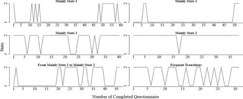
From the individual transition plots of the adolescents (see Figure 5 for six representative examples), we can clearly see between-person differences (that are apparently partly related to clarity and differentiation of emotions). For instance, some adolescents are mainly in the independent state (row 1) and others are mainly in the bipolar state (row 2). However, we can also see some adolescents with frequent transitions between the states (right picture in row 3) and some adolescents with transitions after a certain amount of completed questionnaires (left picture row 3). These transitions indicate that there are likely time-varying within-person variables that influence the transitions but that we are not aware of. Therefore, in the future, it would be interesting if applied researchers would include time-varying covariates in their ESM studies (e.g., stress Dejonckheere, Mestdagh, et al., 2021; Zautra et al., 2002) that could potentially influence within-person changes between a bipolar and an independent representation of one’s emotional state. To conclude, LMFA indicated that configural invariance was violated across states and that some subjects transitioned between the two states frequently over time while others were mainly in one of the two states. Therefore, the questionnaire data is not validly comparable across all subjects and time-points.

Figure 5. Six examples of adolescents’ transition plots that are representative for the whole sample. Note that the scale does not consider the time-interval between the observations to enable the illustration.

Discussion

In this article, we tailored Vermunt’s (2010) maximum likelihood (ML) three-step (3S) procedure to latent Markov factor analysis (LMFA)—a method to explore measurement model (MM) changes over time—and showed that the resulting 3S estimation of LMFA (3S-LMFA) is a promising alternative to the original full information maximum likelihood (FIML) estimation of LMFA (FIML-LMFA): 3S-LMFA performs almost as good as FIML-LMFA, is more accessible and intuitive for applied researchers, and facilitates estimation when researchers want to explore the influence of different (sets of) covariates on transitions between MMs.

It is important to note that this article is one of the first to apply a 3S approach with a continuous-time Markov model to time-intensive longitudinal data, which is data that becomes increasingly popular in different fields with diverse data characteristics. On top of that, the flexible step-wise nature of 3S-LMFA can be used to easily extend the method. Specifically, it is easy to adjust the method to the data and research questions at hand by exchanging the first step (i.e., the mixture factor analysis), which makes it applicable to a wide range of data. For example, one may consider extending item response theory models for longitudinal categorical data. If it is not possible to estimate the first step in Latent GOLD (LG), one can also estimate the first step in a different program and only communicate the results to LG to continue with the second and third step. The same will soon be possible in the open-source program R as we are working on a package that takes estimated state probabilities from any step 1 model (estimated in R or another program) as input, calculates modal state assignments and the classification errors, and links it to an existing package that can estimate single indicator (continuous-time) Markov models with fixed response probabilities. Although adaptations of the MMs are also possible in FIML-LMFA, it is much more difficult in practice since a specific part of the estimation procedure would have to be adapted (i.e., inside the LG software), which is not possible for applied researchers but only for the software programmer.

A limitation of the current paper is that we did not examine the performance of 3S- and FIML-LMFA under violation of the conditional independence assumption and assumed the covariates to influence only the parameters in the structural model (SM), that is, the transitions in the Markov model, and not the factors or the observed variables directly. This assumption might be violated (e.g., being with friends might be related to higher positive affect) and might lead to extracting a wrong number of states and inaccurate parameter estimates (Kim et al., 2016; Kim & Wang, 2017; Masyn, 2017; Nylund-Gibson & Masyn, 2016). As in any other mixture model approach with covariates, the problem of model misspecifications is inherent to both the FIML and the 3S estimation and should be extensively studied in the specific context of LMFA. With regard to extracting the correct number of states, it can be expected that 3S-LMFA performs better than FIML-LMFA when the effects of the covariates on the latent state memberships are included and direct effects of these covariates—for example, on the response variables—are falsely omitted. In the first analysis step of 3S-LMFA, the MMs are formed while disregarding the covariates. Therefore, the covariates do not affect the state enumeration. This is different in FIML-LMFA, where covariates may affect the state enumeration. Specifically, if the local independence assumption is violated, FIML-LMFA would require too many states to counter the local independence violation and achieve a good model fit (Kim & Wang, 2017; Nylund-Gibson & Masyn, 2016). However, inaccurate covariate estimates could occur with both estimation approaches (Asparouhov & Muthén, 2014; Kim et al., 2016; Masyn, 2017). Therefore, it is important to develop diagnostic tools to detect misspecification (e.g., by means of residual statistics) and to account for it, possibly by including the respective covariates with direct effects on the response variables in step 1 of the analysis and by using covariate-specific classification-error adjustments in step 3 (Vermunt & Magidson, 2021). However, tailoring these methods to LMFA is beyond the scope of this paper.

Another limitation is that the states capture not only dynamics in the MM but also in the factor means. If additional states are selected for differences in the factor means, it is difficult to identify if covariates are related to the states only because they explain differences in the MMs or (also) because they explain dynamics in the factor means. In the future, it would be relevant to investigate under which circumstances additional states are selected for factor mean differences and, if necessary, to look into possibilities to lower the impact of factor means on the state formation, for example, by adding random effects to the factor means of zero. This would capture part of the factor mean dynamics and increase the role of other parameter differences in the state formation. Significant covariate effects would then be mainly attributable to differences in the MM parameters.

Article information

Conflict of interest disclosures: Each author signed a form for disclosure of potential conflicts of interest. No authors reported any financial or other conflicts of interest in relation to the work described.

Ethical principles: The authors affirm having followed professional ethical guidelines in preparing this work. These guidelines include obtaining informed consent from human participants, maintaining ethical treatment and respect for the rights of human or animal participants, and ensuring the privacy of participants and their data, such as ensuring that individual participants cannot be identified in reported results or from publicly available original or archival data.

Funding: The research leading to the results reported in this paper was sponsored by the Netherlands Organization for Scientific Research (NWO) [Research Talent grant 406.17.517; Veni grant 451.16.004; Vidi grant 452.17.011].

Role of the funders/sponsors: None of the funders or sponsors of this research had any role in the design and conduct of the study; collection, management, analysis, and interpretation of data; preparation, review, or approval of the manuscript; or decision to submit the manuscript for publication.

Acknowledgments: The ideas and opinions expressed herein are those of the authors alone, and endorsement by the authors’ institutions or the funding agencies is not intended and should not be inferred.

Notes

1 Note that it is also possible to apply LMFA to a single subject if the number of observations was large enough. For guidelines on the required number of observations, see Vogelsmeier, Vermunt, van Roekel, et al. (2019).

2 Note that classifying observations of different subjects into the same latent states entails that persons are assumed to differ from themselves in the same way as persons differ from other persons.

3 This analysis would be comparable to the factor-mean modeling approach that was proposed by Bartolucci and Solis-Trapala (2010).

4 Materials can be found at https://osf.io/svyau.

5 Note that evaluating higher levels of invariances would require specifying increasingly more restrictive confirmatory factor analysis (CFA) models within the states in step 1 of the three-step estimation. Deciding on which equality constrains to add for the loadings may be based on multigroup factor rotation (MGFR; De Roover, Vermunt, & Ceulemans, 2020). For the intercepts and unique variances, the decision can be based on “score tests” (Oberski, van Kollenburg, & Vermunt, 2013). The tenability of (partial) invariance can be evaluated by comparing models with different restrictions, for example, in terms of their BIC value (Lubke & Muthén, 2005). Note that estimating constrained models is already possible in LG but the CFA variant of LMFA with equality restrictions has yet to be explained and evaluated in future research.

6 The method solves the rotation problem for multiple groups simultaneously by rotating group-specific factor loadings to simple structure and between-group agreement with user-defined weights on these two aspects of the rotation.

7 Note that the $\mathbf{Q}$ matrix with the particular structure on the off-diagonals follows naturally from taking the matrix logarithm of the $\mathbf{P}$ matrix with its restriction ${\sum }_{k=1}^K{p}_{\mathit{lk}}=1.$

8 Note that the only difference between time-varying and time-constant covariates is that the former may take different values within a subject (i.e., in the dataset, the covariate scores may differ across rows) and the latter has the same value within a subject (i.e., in the dataset, the covariate scores are repeated/identical across rows).

9 Alternatively, one may also use another EM algorithm in the maximization-step (e.g., McNicholas, 2016).

10 Note that also other assignment rules such as random assignment (Goodman, 2007) can be found in the literature but they are less commonly used for the three-step approaches and are therefore not further discussed.

11 Note that the third step of 3S-LMFA can be fastened by combining the EM estimation with a Newton-Raphson algorithm which is extensively described in De Roover, Vermunt, Timmerman, and Ceulemans (2017).

12 Note that there are many possibilities to manipulate state-separation as previously stated (e.g., number of factors and states and factor overdetermination). For feasibility of the simulation study, we only chose the two types of between-state differences.

13 1.5 hours pertains to one unit and the other intervals are scaled to this unit interval.

14 The population $R_{\mathit{entropy}}^2$ value for a specific choice of population parameters and number of measurement occasions was obtained using Monte Carlo simulation. For this purpose we used the ‘Monte Carlo simulation study’ option in LG with one random draw of the time-intervals and covariate patterns and with the parameters fixed to their population values.

15 Note that it is always good to check the $R_{\mathit{entropy}}^2$ after step 1 that is automatically provided in LG because for a very small state-separation, say, with a value much lower than 0.5, it might be better to conduct a FIML-LMFA with additional state-separation information from the SM (including covariates). This is because in that case, the actual differences between the states might be even lower than the estimated ones. This would lead to an underestimation of the classification error (Vermunt, 2010). However, such low values are unlikely to be found in practice.

16 Note that we also investigated whether the solutions converged to local maxima (i.e., that they had smaller $\log L$ values than the global maximum likelihood (ML) solution. Although the latter is unknown, we can obtain an approximation (‘proxi’) in simulation studies by estimating the models with the population parameters as starting values. When ${\log L}_{\mathit{multistart}}<{\log L}_{\mathit{proxi}},$ the solution is considered a local maximum. This was no issue in FIML-LMFA and the first step of 3S-LMFA and only occurred for 3 datasets in the third step of 3S-LMFA.

17 Note that the rotation was done in R. Although rotation in LG was already possible for known groups, the issue with switching state labels has to be resolved to provide LG with the correct state-specific target matrices before rotation can be applied to unknown groups such as the states.

18 The unique variance recovery may be affected by Heywood cases (i.e., improper factor solutions with at least one unique variance being negative or equal to zero, possibly caused by insufficient amount of information or underdetermined factors; Van Driel, 1978). However, this was not the case in any of the analyses.

19 Note that the NA items were generally right-skewed. Since the consequences of violating the normality assumption have yet to be investigated, one should be particularly cautious with drawing substantial conclusions (Vogelsmeier, Vermunt, van Roekel, et al., 2019). This is, however, not a problem for illustrating the purpose of 3S-LMFA.

20 Note that three subjects in the ESM study did not have any baseline measures for an unspecified reason. For such cases, LG automatically imputes the average scale score.

21 Note that we did not add covariates to the initial state probabilities as the number of subjects was rather small.

 

Appendix

A.1 Derivations

A.1.1 Derivation step 2

We obtain the conditional probabilities, $p\left(w_{\mathit{itm}}=1|s_{\mathit{itk}}=1\right),$ starting from the joint probability $p\left(w_{\mathit{itm}}=1,s_{\mathit{itk}}=1,{\mathbf{y}}_{\mathit{it}}\right)$ applying the product rule: (A1) $$p\left(w_{itm}=1,s_{itk}=1,y_{it}\right)=p\left(w_{itm}=1|s_{itk}=1,y_{it}\right)\times p\left(y_{it}|s_{itk}=1\right)p\left(s_{itk}=1\right)$$(A1) .

Next, conditioning on $s_{\mathit{itk}}=1$ yields (A2) $$p\left(w_{\mathit{itm}}=1,{\mathbf{y}}_{\mathit{it}}|s_{\mathit{itk}}=1\right)=p\left(w_{\mathit{itm}}=1|s_{\mathit{itk}}=1,{\mathbf{y}}_{\mathit{it}}\right)p\left({\mathbf{y}}_{\mathit{it}}|s_{\mathit{itk}}=1\right)=p\left(w_{\mathit{itm}}=1|{\mathbf{y}}_{\mathit{it}}\right)p\left({\mathbf{y}}_{\mathit{it}}|s_{\mathit{itk}}=1\right)$$(A2) because $w_{\mathit{itm}}=1$ is conditionally independent of $s_{\mathit{itk}}=1$ given ${\mathbf{y}}_{\mathit{it}}$ (see Figure 3). Next, we obtain the marginal probability by integrating out ${\mathbf{y}}_{\mathit{it}}:$ (A3) $$p\left(w_{\mathit{itm}}=1|s_{\mathit{itk}}=1\right)=\int p\left(w_{\mathit{itm}}=1|{\mathbf{y}}_{\mathit{it}}\right)p\left({\mathbf{y}}_{\mathit{it}}|s_{\mathit{itk}}=1\right)d{\mathbf{y}}_{\mathit{it}},$$(A3) where the second factor on the right-hand side$$ can be rewritten using Bayes’ theorem: (A4) $$p\left({\mathbf{y}}_{\mathit{it}}|s_{\mathit{itk}}=1\right)=\frac{p\left({\mathbf{y}}_{\mathit{it}}\right)p\left(s_{\mathit{itk}}=1|{\mathbf{y}}_{\mathit{it}}\right)}{p\left(s_{\mathit{itk}}=1\right)}.$$(A4)

Inserting this in Eq. (A3)(A3) $$p\left(w_{\mathit{itm}}=1|s_{\mathit{itk}}=1\right)=\int p\left(w_{\mathit{itm}}=1|{\mathbf{y}}_{\mathit{it}}\right)p\left({\mathbf{y}}_{\mathit{it}}|s_{\mathit{itk}}=1\right)d{\mathbf{y}}_{\mathit{it}},$$(A3) leads to (A5) $$p\left(w_{\mathit{itm}}=1|s_{\mathit{itk}}=1\right)=\frac{\int p\left(w_{\mathit{itm}}=1|{\mathbf{y}}_{\mathit{it}}\right)p\left({\mathbf{y}}_{\mathit{it}}\right)p\left(s_{\mathit{itk}}=1|{\mathbf{y}}_{\mathit{it}}\right)d{\mathbf{y}}_{\mathit{it}}}{p\left(s_{\mathit{itk}}=1\right)},$$(A5) where $p\left(s_{\mathit{itk}}=1\right)$ is factored out from the integral because it is independent of ${\mathbf{y}}_{\mathit{it}}.$

A.1.2 Derivation step 3

We consider the joint probability and solve for $p({\mathbf{W}}_i|{\mathbf{Z}}_i).$ The joint probability is (A6) $$p\left({\mathbf{W}}_i,{\mathbf{Y}}_i,{\mathbf{S}}_i,{\mathbf{Z}}_i\right)=p\left({\mathbf{W}}_i\right|{\mathbf{Y}}_i,{\mathbf{S}}_i,{\mathbf{Z}}_i\left)p\right({\mathbf{Y}}_i\left|{\mathbf{S}}_i,{\mathbf{Z}}_i\right)p\left({\mathbf{S}}_i\right|{\mathbf{Z}}_i\left)p\right({\mathbf{Z}}_i).$$(A6)

Next, we condition on ${\mathbf{Z}}_i$ and use the assumption that ${\mathbf{Z}}_i$ and ${\mathbf{Y}}_i$ are conditionally independent given ${\mathbf{S}}_i$ and that ${\mathbf{W}}_i$ is conditionally independent of ${\mathbf{S}}_i$ and ${\mathbf{Z}}_i$ given ${\mathbf{Y}}_i,$ which is also depicted in Figure 4: (A7) $$\begin{array}{c}p\left({\mathbf{W}}_i,{\mathbf{Y}}_i,{\mathbf{S}}_i|{\mathbf{Z}}_i\right)=p\left({\mathbf{W}}_i\right|{\mathbf{Y}}_i\left)p\right({\mathbf{Y}}_i\left|{\mathbf{S}}_i\right)p\left({\mathbf{S}}_i\right|{\mathbf{Z}}_i)\\ =p\left({\mathbf{w}}_{i1}\right|{\mathbf{y}}_{i1})\cdots p({\mathbf{w}}_{iT}\left|{\mathbf{y}}_{\mathit{iT}}\right)p\left({\mathbf{y}}_{i1}\right|{\mathbf{s}}_{i1})\cdots p({\mathbf{y}}_{\mathit{iT}}\left|{\mathbf{s}}_{iT}\right)p\left({\mathbf{s}}_{i1},\dots ,{\mathbf{s}}_{iT}\right|{\mathbf{z}}_{i1},\dots {,\mathbf{z}}_{iT})\\ =p\left({\mathbf{y}}_{i1}\right|{\mathbf{s}}_{i1}\left)p\right({\mathbf{w}}_{i1}\left|{\mathbf{y}}_{i1}\right)\cdots p\left({\mathbf{y}}_{\mathit{iT}}\right|{\mathbf{s}}_{iT}\left)p\right({\mathbf{w}}_{iT}\left|{\mathbf{y}}_{\mathit{iT}}\right)\times \stackrel{\mathit{Markov}\mathit{Chain}\left(MC\right)}{\overbrace{p\left({\mathbf{s}}_{i1}\right|{\mathbf{z}}_{i1}\left)p\right({\mathbf{s}}_{i2}\left|{{\mathbf{s}}_{i1},\mathbf{z}}_{i2}\right)\cdots p\left({\mathbf{s}}_{iT}\right|{{\mathbf{s}}_{iT¯1},\mathbf{z}}_{iT})}},\end{array}$$(A7) where we use $p\left({\mathbf{w}}_{it}\right|{\mathbf{y}}_{\mathit{it}})$ with the $m$ th element in ${\mathbf{w}}_{it}$ equal to 1 and all others equal to 0 as a shorthand notation for $p\left(w_{\mathit{itm}}=1|{\mathbf{y}}_{\mathit{it}}\right).$ We then marginalize over ${\mathbf{S}}_i$ and ${\mathbf{Y}}_i:$ (A8) $$p\left({\mathbf{W}}_i\right|{\mathbf{Z}}_i)=\sum _{{\mathbf{s}}_{i1}}\cdots \sum _{{\mathbf{s}}_{iT}}\int p\left({\mathbf{y}}_{i1}\right|{\mathbf{s}}_{i1}\left)p\right({\mathbf{w}}_{i1}\left|{\mathbf{y}}_{i1}\right)d{\mathbf{y}}_{\mathit{it}}\cdots \int p\left({\mathbf{y}}_{\mathit{iT}}\right|{\mathbf{s}}_{iT}\left)p\right({\mathbf{w}}_{iT}\left|{\mathbf{y}}_{\mathit{iT}}\right)d{\mathbf{y}}_{\mathit{it}}\times MC$$(A8)

We can then rewrite $p\left({\mathbf{y}}_{\mathit{it}}|{\mathbf{s}}_{it}\right)$ using Bayes’ theorem (see A4), insert it in Eq. (A8)(A8) $$p\left({\mathbf{W}}_i\right|{\mathbf{Z}}_i)=\sum _{{\mathbf{s}}_{i1}}\cdots \sum _{{\mathbf{s}}_{iT}}\int p\left({\mathbf{y}}_{i1}\right|{\mathbf{s}}_{i1}\left)p\right({\mathbf{w}}_{i1}\left|{\mathbf{y}}_{i1}\right)d{\mathbf{y}}_{\mathit{it}}\cdots \int p\left({\mathbf{y}}_{\mathit{iT}}\right|{\mathbf{s}}_{iT}\left)p\right({\mathbf{w}}_{iT}\left|{\mathbf{y}}_{\mathit{iT}}\right)d{\mathbf{y}}_{\mathit{it}}\times MC$$(A8) , and make use of (A5), which leads to (A9) $$\begin{array}{c}p\left({\mathbf{W}}_i\right|{\mathbf{Z}}_i)=\sum _{{\mathbf{s}}_{i1}}\cdots \sum _{{\mathbf{s}}_{iT}}\stackrel{\mathit{classification} \mathit{error} }{\overbrace{\frac{\int p\left({\mathbf{s}}_{i1}\right|{\mathbf{y}}_{i1}\left)p\right({\mathbf{y}}_{i1}\left)p\right({\mathbf{w}}_{i1}\left|{\mathbf{y}}_{i1}\right)d{\mathbf{y}}_{i1}}{p\left({\mathbf{s}}_{i1}\right)}}}\cdots \stackrel{\mathit{classification} \mathit{error} }{\overbrace{\frac{\int p\left({\mathbf{s}}_{iT}\right|{\mathbf{y}}_{iT}\left)p\right({\mathbf{y}}_{iT}\left)p\right({\mathbf{w}}_{iT}\left|{\mathbf{y}}_{iT}\right)d{\mathbf{y}}_{iT}}{p\left({\mathbf{s}}_{iT}\right)}}}\times MC\\ \begin{array}{c}=\sum _{{\mathbf{s}}_{i1}}\cdots \sum _{{\mathbf{s}}_{iT}}p\left({\mathbf{w}}_{i1}|{\mathbf{s}}_{i1}\right)\cdots p\left({\mathbf{w}}_{iT}|{\mathbf{s}}_{iT}\right)\times MC\\ =\sum _{{\mathbf{s}}_{i1}}\cdots \sum _{{\mathbf{s}}_{iT}}p\left({\mathbf{s}}_{i1}\right|{\mathbf{z}}_{i1})\prod _{t=2}^{T}p\left({\mathbf{s}}_{it}\right|{{\mathbf{s}}_{it-1},\mathbf{z}}_{it})\prod _{t=1}^{T}p\left({\mathbf{w}}_{it}|{\mathbf{s}}_{it}\right).\end{array}\end{array}$$(A9)

A.2 Additional simulation study: Autocorrelated factor scores

A.2.1 Problem

In order to investigate whether ignoring autocorrelated factor scores is more harmful for the performance of 3S-LMFA than it is for FIML-LMFA (Vogelsmeier, Vermunt, van Roekel, & De Roover, 2019), we conducted a simulation study with selected conditions from the main simulation study (a–d) and, furthermore, manipulated the autocorrelation (e). More specifically, we kept the state-separation conditions (a) and (b) as they had considerable effects on the performances in the main simulation study (Section “Simulation Study”) but we kept respectively only one factor of the conditions pertaining to the amount of information (c and d) as these conditions had only minor effects on the performances. For the size of the autocorrelation, we used the coefficients suggested by Cabrieto et al. (2017), that were also used in the simulation study to investigate the effect of ignoring autocorrelation in FIML-LMFA (Vogelsmeier, Vermunt, van Roekel, & De Roover, 2019).

A.2.2 Design and procedure

The new conditions were the following: $$\begin{array}{cc}\text{State‐separation}& \{\begin{array}{l}\text{a}\text{.\hspace{0.17em}\hspace{0.17em}Between}‐\text{state\hspace{0.17em}\hspace{0.17em}loading\hspace{0.17em}\hspace{0.17em}differences\hspace{0.17em}\hspace{0.17em}at\hspace{0.17em}\hspace{0.17em}two\hspace{0.17em}\hspace{0.17em}levels}:\\ \text{medium\hspace{0.17em}\hspace{0.17em}loading\hspace{0.17em}\hspace{0.17em}differences},\text{\hspace{0.17em}\hspace{0.17em}low\hspace{0.17em}\hspace{0.17em}loading\hspace{0.17em}\hspace{0.17em}differences};\\ \text{b}\text{.\hspace{0.17em}\hspace{0.17em}Between}‐\text{state\hspace{0.17em}\hspace{0.17em}intercept\hspace{0.17em}\hspace{0.17em}differences\hspace{0.17em}\hspace{0.17em}at\hspace{0.17em}\hspace{0.17em}two\hspace{0.17em}\hspace{0.17em}levels}:\\ \text{no\hspace{0.17em}\hspace{0.17em}intercept\hspace{0.17em}\hspace{0.17em}differences},\text{\hspace{0.17em}\hspace{0.17em}low\hspace{0.17em}\hspace{0.17em}intercept\hspace{0.17em}\hspace{0.17em}differences};\end{array}\end{array}\begin{array}{cc}\text{Amount\hspace{0.17em}\hspace{0.17em}of\hspace{0.17em}\hspace{0.17em}information}& \{\begin{array}{l}\text{c}\text{.\hspace{0.17em}\hspace{0.17em}Fixed\hspace{0.17em}\hspace{0.17em}number\hspace{0.17em}\hspace{0.17em}of\hspace{0.17em}\hspace{0.17em}subjects\hspace{0.17em}\hspace{0.17em}}N:70*;\\ \text{d}\text{.\hspace{0.17em}\hspace{0.17em}Fixed\hspace{0.17em}\hspace{0.17em}Number\hspace{0.17em}\hspace{0.17em}of\hspace{0.17em}\hspace{0.17em}days\hspace{0.17em}\hspace{0.17em}}D:70*\\ \text{e}\text{.\hspace{0.17em}\hspace{0.17em}Autocorrelation\hspace{0.17em}\hspace{0.17em}at\hspace{0.17em}\hspace{0.17em}three\hspace{0.17em}\hspace{0.17em}levels}:0,0.\text{3},0.\text{7}\end{array}\end{array}$$

The conditions marked with “*” are the ones that are the ones that are now fixed to one value from the manipulated conditions in the main simulation study. This design resulted in $2\times 2\times 1\times 1\times 3=12$ conditions. The data generation was the same as in the main simulation study (again with 100 replicates). However, instead of using an orthogonal regular factor model as shown in Eq. (1)(1) $$\left[{\mathbf{y}}_{it}\right|s_{\mathit{itk}}=1]= {\mathbf{\nu }}_k+{\mathbf{\Lambda }}_k {\mathbf{f}}_{\mathit{itk}}+ {\mathbf{e}}_{\mathit{itk}}.$$(1) , we used an orthogonal dynamic factor model, where the factor scores at time-point $t$ are correlated with the factor scores at $t-1$ by the coefficient $\varphi$ (e): $${\mathbf{y}}_{it}=\mathrm{\hspace{0.17em}\hspace{0.17em}}{\mathbf{\nu }}_k+{\mathbf{\Lambda }}_k\mathrm{\hspace{0.17em}\hspace{0.17em}}{\mathbf{f}}_{\mathit{itk}}+\mathrm{\hspace{0.17em}\hspace{0.17em}}{\mathbf{e}}_{it}$$ (A10) $${\mathbf{f}}_{\mathit{it}}={\mathbf{\varphi }\mathbf{f}}_{\mathit{it}-1,k}+{\mathbf{\epsilon }}_{it},$$(A10) where ${\mathbf{\epsilon }}_{it}\sim \mathit{MVN}(\mathbf{0},\mathbf{I})$ is a subject- and time-point specific $F_k\times 1$ noise vector. The correlated factor scores ${\mathbf{f}}_{\mathit{itk}}$ were generated by means of a recursive filter (Hamilton, 1994), that is, the first factor scores are set equal to the noise elements ${\mathbf{\epsilon }}_{i1}$ and the remaining scores are computed as in Eq. (A10)(A10) $${\mathbf{f}}_{\mathit{it}}={\mathbf{\varphi }\mathbf{f}}_{\mathit{it}-1,k}+{\mathbf{\epsilon }}_{it},$$(A10) . In order to retain the expected variance of 1, we multiplied the resulting factor scores by $\sqrt{1-{\varphi }^2}$ (De Roover et al., 2014). Note that we computed the average autocorrelation across all datasets belonging to the same condition to see how the manipulation played out. The autocorrelations were −0.02, 0.26, and 0.64.

A.2.3 Results

Overall, the state recovery and the parameter recovery of the MMs was unaffected for both 3S- and FIML-LMFA (Table A1). Only the state recovery after step 3 of 3S-LMFA was slightly worse for increasing autocorrelations. Furthermore, with both procedures, the intercept recovery decreased for increasing autocorrelations. This is because the autocorrelations are partly captured by the intercepts and in turn have a higher variation around the population values.

Regarding the SM (Table A2), the recovery was also largely unaffected for both 3S- and FIML-LMFA. Only for the strongest autocorrelation ($\varphi =.7$) in 3S-LMFA, the RMSE was slightly higher and the SEs slightly more underestimated for the initial state intercepts and the bias was slightly higher for the transition intercepts. Thus, the autocorrelation appears to be partially captured by the step-3 latent state transitions. However, the effect of the autocorrelation on the parameter estimation is negligible.

Table A1. Goodness of recovery for the states, loadings, intercepts and unique variances conditional on the three autocorrelation factors.

		Goodness of recovery
		States $(\mathit{ARI})$			States RI $(RI)$			Loadings $(\mathit{GOSL})$		Intercepts $({\mathit{MAD}}_{\mathit{int}})$		Unique Variances $({\mathit{MAD}}_{\mathit{unique}})$
		Type of LMFA
Condition	Factors	3S-1	3S-3	FIML	3S-1	3S-3	FIML	3S	FIML	3S	FIML	3S	FIML
Auto-correlation $\varphi$	0	.61	.87	.94	.82	.94	.97	1	1	.02	.02	.01	.01
	.3	.61	.86	.94	.82	.94	.97	1	1	.03	.03	.01	.01
	.7	.61	.85	.93	.82	.93	.97	1	1	.04	.04	.01	.01

Note. LMFA = latent Markov factor analysis; 3S-1 = three-step step 1; 3S-3 = three-step step 3; FIML = full information maximum likelihood. The perfect loading recoveries result from the loading matrices that are highly similar across the states.

Table A2. Parameter Bias, RMSE, and SE/SD for the four types of parameters averaged across and conditional on the three autocorrelation factors.

		Initial state intercept parameters			Transition intercept parameters			Slope parameters covariate 1			Slope parameters covariate 2
		Bias	RMSE	SE/SD	Bias	RMSE	SE/SD	Bias	RMSE	SE/SD	Bias	RMSE	SE/SD
Condition	Factor	FIML-LMFA
	Average	.01	.31	1.01	−.02	.18	1	−.01	.18	0.99	0	.17	0.99
Auto-correlation $\varphi$	0	.02	.31	1.01	−.02	.18	1.01	0	.18	0.98	0	.17	0.97
	.3	.01	.31	1.02	−.02	.18	1.01	0	.18	0.98	0	.17	0.99
	.7	0	.32	1.01	−.02	.19	0.99	−.01	.18	1	0	.17	1
Condition	Factor	3S-LMFA
	Average	.01	.35	0.98	.01	.23	0.98	0	.23	0.95	0	.20	0.96
Auto-correlation $\varphi$	0	0	.33	1	0	.23	0.99	−.01	.23	0.94	−.01	.20	0.96
	.3	0	.33	1	−.01	.23	0.99	−.01	.23	0.94	0	.21	0.95
	.7	.02	.37	0.94	.04	.23	0.97	0	.22	0.97	0	.20	0.97

Note. LMFA = latent Markov factor analysis; FIML = full information maximum likelihood; 3S = three-step.

A.3 Additional simulation study: Varying covariate distributions and effects

A.3.1 Problem

In order to test whether non-uniform covariate distributions and the strength of the covariate effects influence the performance of 3S- and FIML-LMFA differently, we repeated selected conditions from the main simulation study and additionally manipulated the strength of the covariate effects (e) and the distribution of covariates (f). More specifically, we selected the conditions that affected the performances in the main simulation study the most (Section “Simulation Study”). This implied that we kept the state-separation conditions (a and b) while selecting only one factor from the conditions pertaining to the amount of information (c and d).

A.3.2 Design and procedure

The new conditions were the following: $$\begin{array}{cc}\text{State‐separation}& \{\begin{array}{l}\text{a}\text{.\hspace{0.17em}\hspace{0.17em}Between}‐\text{state\hspace{0.17em}\hspace{0.17em}loading\hspace{0.17em}\hspace{0.17em}differences\hspace{0.17em}\hspace{0.17em}at\hspace{0.17em}\hspace{0.17em}two\hspace{0.17em}\hspace{0.17em}levels}:\\ \text{medium\hspace{0.17em}\hspace{0.17em}loading\hspace{0.17em}\hspace{0.17em}differences},\text{\hspace{0.17em}\hspace{0.17em}low\hspace{0.17em}\hspace{0.17em}loading\hspace{0.17em}\hspace{0.17em}differences};\\ \text{b}\text{.\hspace{0.17em}\hspace{0.17em}Between}‐\text{state\hspace{0.17em}\hspace{0.17em}intercept\hspace{0.17em}\hspace{0.17em}differences\hspace{0.17em}\hspace{0.17em}at\hspace{0.17em}\hspace{0.17em}two\hspace{0.17em}\hspace{0.17em}levels}:\\ \text{no\hspace{0.17em}\hspace{0.17em}intercept\hspace{0.17em}\hspace{0.17em}differences},\text{\hspace{0.17em}\hspace{0.17em}low\hspace{0.17em}\hspace{0.17em}intercept\hspace{0.17em}\hspace{0.17em}differences};\end{array}\end{array}\begin{array}{cc}\text{Amount\hspace{0.17em}\hspace{0.17em}of\hspace{0.17em}\hspace{0.17em}information}& \{\begin{array}{l}\text{c}\text{.}\text{Number\hspace{0.17em}\hspace{0.17em}of\hspace{0.17em}\hspace{0.17em}Subjects\hspace{0.17em}\hspace{0.17em}}N\text{\hspace{0.17em}\hspace{0.17em}at\hspace{0.17em}\hspace{0.17em}four\hspace{0.17em}\hspace{0.17em}levels}:70*;\\ \text{d}\text{.\hspace{0.17em}\hspace{0.17em}Number\hspace{0.17em}\hspace{0.17em}of\hspace{0.17em}\hspace{0.17em}days\hspace{0.17em}\hspace{0.17em}}D\text{\hspace{0.17em}\hspace{0.17em}at\hspace{0.17em}\hspace{0.17em}two\hspace{0.17em}\hspace{0.17em}levels}:7*;\\ \text{e}\text{.}\text{Strength\hspace{0.17em}\hspace{0.17em}of\hspace{0.17em}\hspace{0.17em}covariate\hspace{0.17em}\hspace{0.17em}effects}\hspace{0.17em}\hspace{0.17em}\text{at\hspace{0.17em}\hspace{0.17em}three\hspace{0.17em}\hspace{0.17em}levels}:0.\text{25},0.\text{5},\text{\hspace{0.17em}\hspace{0.17em}1}\\ \text{f}\text{.\hspace{0.17em}\hspace{0.17em}Distributions\hspace{0.17em}\hspace{0.17em}of\hspace{0.17em}\hspace{0.17em}covariate\hspace{0.17em}\hspace{0.17em}scores\hspace{0.17em}\hspace{0.17em}at\hspace{0.17em}\hspace{0.17em}three\hspace{0.17em}\hspace{0.17em}levels}:\text{7}0/\text{3}0,\text{\hspace{0.17em}\hspace{0.17em}5}0/\text{5}0,\text{\hspace{0.17em}\hspace{0.17em}3}0/\text{7}0\end{array}\end{array}$$

The conditions marked with “*” are the ones that are now fixed to one value from the main simulation study. This design resulted in $2\times 2\times 1\times 1\times 3\times 3=36$ conditions. We generated the data as in the main simulation study (again with 100 replicates). However, the effects of the time-varying covariate $z_{it1}$ and time-constant covariate $z_{i2}$ as well as their distributions across observations and/or subjects differed depending on factors (e) and (f). First, with regard to the strength of the covariate effects, a higher value for $z_{it1}$ still lowered the probabilities of transitioning to and staying in state 1 and 3 and increased the probabilities of transitioning to and staying in state 2 but with slope parameters being equal to ${\gamma }_{12,z_{it1}}={\gamma }_{32,z_{it1}}=1$ and ${\gamma }_{13,z_{it1}}={\gamma }_{21,z_{it1}}={\gamma }_{23,z_{it1}}={\gamma }_{31,z_{it1}}=-\tau .$ Furthermore, a higher value for $z_{i2}$ still increased the probability to transition away from the origin state but with slope parameters being equal to ${\gamma }_{12,z_{it2}}={\gamma }_{13,z_{it2}}={\gamma }_{21,z_{it2}}={\gamma }_{23,z_{it2}}={\gamma }_{31,z_{it2}}={\gamma }_{32,z_{it2}}=\tau .$ The parameter τ was either 0.25, 0.5, or 1 (see factor e).

Next, with regard to the distributions of the covariate scores $-0.5$ and $0.5,$ we included conditions with a uniform distribution (i.e., “50/50”) and both a “70/30” and “30/70” condition. The time-varying covariate $z_{it1}$ was assigned such that the score changed from $-0.5$ to $0.5$ after 5 of the 7 days in the 70/30 condition and after 2 days in the 30/70 condition. To obtain exactly a 50/50 condition, the scores changed after 3 days for the first half of the subjects and after 4 days for the other half of the subjects. For the time-constant covariate $z_{i2},$ the scores $-0.5$ and $0.5$ were randomly selected with probabilities being equal to the three distribution levels (i.e., 70/30, 50/50, or 30/70). Note that we included a 70/30 and 30/70 condition to prevent a possible confounding of the results: The covariate scores influence the transition probabilities (i.e., the state memberships become more or less stable) and a higher stability of the state membership previously showed a positive influence on the recovery of the states in FIML-LMFA (Vogelsmeier, Vermunt, van Roekel, & De Roover, 2019). For instance, a covariate score of $-0.5$ on both covariates would lead to a slightly more stable transition probability matrix than a covariate score of $0.5$ on both covariates (e.g., with an average of 96% versus 92% probability to stay in a state with $\tau =1$ and a one-unit interval). Note, however, that the difference is so small that it might not affect the performance.

A.3.3 Results

The results can be found in Table A3. The state and MM recovery of 3S- and FIML-LMFA were largely unaffected by the strength of the effect and the distribution of the covariates and, therefore, will not be further discussed. With regard to the SM, there was only a very small effect with regard to the RMSE but it was the same for both estimation procedures. First, the RMSE was slightly higher for the strongest covariate effect (i.e., $\tau =1$). This is likely due to somewhat larger SE values that are inherent to larger logit parameters. Second, the RMSE for the transition intercepts and transition slopes was slightly higher for non-uniform covariate distributions, which is likely caused by the general loss of information when covariate scores are not uniformly distributed.

Table A3. Parameter Bias, RMSE, and SE/SD for the four types of parameters averaged across and conditional on the manipulated factors.

		Initial state intercept parameters			Transition intercept parameters			Slope parameters covariate 1			Slope parameters covariate 2
		Bias	RMSE	SE/SD	Bias	RMSE	SE/SD	Bias	RMSE	SE/SD	Bias	RMSE	SE/SD
Condition	Factor	FIML-LMFA
	Average	.01	.31	1.02	−.03	.22	0.98	0	.2	0.98	0	.18	0.98
Strength of covariate effects $\tau$	0.25	.01	.30	1.02	−.03	.21	0.98	−.01	.2	0.97	0	.18	0.98
	0.50	0	.30	1.04	−.02	.21	0.98	0	.2	0.99	0	.18	0.99
	1.00	.02	.32	1	−.03	.23	0.99	0	.21	0.99	−.01	.19	0.97
Distributions of covariate scores	30/70	0	.31	1.01	−.03	.24	0.99	−.02	.21	0.98	−.02	.2	0.98
	50/50	.02	.31	1.02	−.02	.19	0.98	0	.18	0.99	0	.17	0.98
	70/30	.02	.30	1.03	−.03	.22	0.98	.01	.21	0.99	0	.18	0.98
	Factor	3S−LMFA
	Average	.01	.34	1	−.02	.28	0.98	0	.26	0.97	0	.22	0.96
Strength of covariate effects $\tau$	0.25	.02	.33	1.01	−.02	.27	0.98	−.01	.25	0.96	0	.22	0.97
	0.50	.01	.33	1	−.01	.27	0.98	0	.25	0.97	0	.22	0.97
	1.00	0	.34	1	−.02	.30	0.99	.01	.28	0.98	−.01	.24	0.94
Distributions of covariate scores	30/70	.01	.34	0.99	−.02	.31	0.99	−.02	.27	0.98	−.02	.25	0.96
	50/50	−.01	.34	1	−.01	.23	0.97	0	.23	0.96	0	.2	0.96
	70/30	.01	.33	1.02	−.02	.28	0.99	.02	.27	0.98	0	.22	0.95

Note. LMFA = latent Markov factor analysis; FIML = full information maximum likelihood; 3S = three-step.

A.4 Step 1 and 2 syntax of 3S-LMFA

//LG5.1//version = 5.1infile 'Dataset.csv' quote = singlemodeltitle 'Step 1 and Sep 2 CT-[2 2 2]';options algorithm tolerance = 1e-008 emtolerance = 1e-008 emiterations = 5000 nriterations = 0; startvalues seed = 0 sets = 25 tolerance = 1e-005 iterations = 100 PCA; bayes latent = 1 categorical = 1 poisson = 1 variances = 1; quadrature nodes = 10; missing includeall; output parameters = effect betaopts = wl standarderrors classification profile probmeans = posterior bivariateresiduals estimatedvalues = model iterationdetails WriteParameters = 'results_parameters1.csv' write = 'results1.csv'; outfile 'classification1.csv' classification keep id deltaT cov1_vary_D cov2_con_N; variables dependent V1 continuous,V2 continuous,V3 continuous,V4 continuous,V5 continuous,V6 continuous,V7 continuous,V8 continuous,V9 continuous,V10 continuous, V11 continuous, V12 continuous,V13 continuous, V14 continuous, V15 continuous, V16 continuous, V17 continuous, V18 continuous, V19 continuous, V20 continuous; latent State nominal coding = first 3, F1 continuous, F2 continuous; equations (1) F1| State; (1) F2| State; State <- 1 ; V1-V20 <- 1 | State + F1 | State + F2 | State; V1 | State; V2 | State; V3 | State; V4 | State; V5 | State; V6 | State; V7 | State; V8 | State; V9 | State; V10 | State; V11 | State; V12 | State; V13 | State; V14 | State; V15 | State; V16 | State; V17 | State; V18 | State; V19 | State; V20 | State;end model

A.5 Step 3 syntax of 3S-LMFA

Note that the step-3 syntax below is only one option to estimate the third step. Instead of calculating the classification error probability matrix manually and inserting it into the syntax ('w = …') to tell LG that the matrix should be used as fixed response probability matrix, it is also possible to use the “step3” option in LG ('step3 ml modal;'). When using this option, LG automatically calculates the classification error probability matrix from the input file (i.e., the step 1 posterior probabilities and the modal state assignments, here 'classification1.csv') and uses it as fixed response probability matrix. However, when using the step3 option, LG does not yet provide the user with the final latent state-assignments. This is because the classification is often not the primary focus of interest in other three-step analyses where researchers rather focus on parameter estimates such as covariate effects. Since classification is certainly of interest in LMFA, we suggest to use the manual syntax version.

//LG5.1//version = 5.1infile 'classification1.csv' quote = singlemodeltitle 'Step 3-[2 2 2]';options algorithm tolerance = 1e-008 emtolerance = 1e-006 emiterations = 5000 nriterations = 500 expm = pade; startvalues seed = 0 sets = 25 tolerance = 1e-005 iterations = 100 PCA; bayes latent = 1 categorical = 1 poisson = 1 variances = 1 ct = 1;quadrature nodes = 10; missing includeall; output parameters = effect standarderrors classification profile iterationdetails estimatedvalues = model WriteParameters = 'results_parameters2.csv' write = 'results2.csv'; outfile 'classification2.csv' classification; variables caseid id; independent cov1_vary_D nominal, cov2_con_N nominal; timeinterval deltaT; latent State3 nominal dynamic coding = first 3; dependent State#; equations State3[=0] <- 1; State3 <- (∼tra) 1 | State3[-1] + (∼tra) cov1_vary_D | State3[-1] + (∼tra) cov2_con_N | State3[-1]; State# <- (w ∼ wei) State3;w= values obtained from first syntax;end model

A.6 Extra information application

A.6.1 Model selection procedure with the CHull method

For the model selection, we ran all models five times to see whether the maximum likelihood solutions were indeed global solutions. We considered the solutions to be global when the absolute differences between the loglikelihood values of the 5 solutions was respectively smaller than 0.01. As a result, 11 out of 19 models were passed to the model selection procedure with the CHull method, which was conducted with the R-package “multichull” (note that we also did a sensitivity check by doing the CHull test including possible local optima and the selected model was always the same). The CHull can be considered an automated generalized scree-test (Bulteel et  al., 2013; Ceulemans & Kiers, 2006; Ceulemans & Van Mechelen, 2005). The method identifies the models in a “loglikelihood versus number of parameters” plot that are at the higher boundary of the convex hull (Cattell, 1966) and identifies the optimal model by evaluating the elbow in the scree plot (i.e., the point where the improvement in fit with additional parameters levels off). During the CHull procedure, following Wilderjans et al. (2013)’s recommendation, we discarded models for which the fit was almost equal to the fit of a less complex model (i.e., when it fitted less than 1 percent better than the less complex model, which is also the default value in the R-package). The model with 2 states and respectively 2 and 1 factors (“[2 1]”) was the best (see output in A.6.2). The second best model was the model with two states and 1 factor in both states (“[1 1]”). From the grouping of points, corresponding to the different number of states, it can also be seen that the improvement in fit from 1 to 2 states is much larger than the one from 2 to 3 states. Model [2 1] was also better than model [1 1] according to the BIC values (see output A.6.3) and furthermore, better interpretable (model [1 1] was comparable to model [2 1] only that the second factor in the first state was clearly missing as was evident from tremendously high unique variance proportions for the items that had high loadings on the second factor in model [2 1]. Therefore, for this application, we chose model [2 1].

A.6.2 Output CHull

Output from the CHull method performed by the R-package “multichull “shows the models considered, the models on the upper bound of the convex hull, the selected model [2 1], and the CHull-figure plotting the number of free parameters against the loglikelihood value.

SETTINGS BY USER:Optimalization: upper boundRequired improvement in fit: 1%Number of considered models: 11 RESULTS:Number of selected models: 1 SELECTED MODEL: complexity fit[2 1] 71 -41695.7 ALL MODELS ON upper BOUND: complexity fit st[1] 30 -48338.88 NA[1 1] 61 -42738.06 1.733280[2 1] 71 -41695.70 2.572494[1 1 1] 92 -40844.78 NA ORIGINAL MODELS complexity fit[1] 30 -48338.88[2] 40 -47601.71[3] 50 -47468.42[1 1] 61 -42738.06[2 1] 71 -41695.70[2 2] 81 -41477.40[3 2] 91 -41430.23[1 1 1] 92 -40844.78[3 3] 101 -41406.83[2 1 1] 102 -40495.49[3 2 1] 122 -40367.42

A.6.3 Output BIC

This is an extra BIC-figure that, comparable to the CHull-figure, plots the number of free parameters against the BIC value, showing that model [2 1] fits considerably better than model [1 1] not only according to the CHull but also according to the BIC value.

References

- Asparouhov, T., & Muthén, B. (2014). Auxiliary variables in mixture modeling: Three-step approaches using Mplus. Structural Equation Modeling: A Multidisciplinary Journal, 21(3), 329–341. https://doi.org/10.1080/10705511.2014.915181
- Bakk, Z., Tekle, F. B., & Vermunt, J. K. (2013). Estimating the association between latent class membership and external variables using bias-adjusted three-step approaches. Sociological Methodology, 43(1), 272–311. https://doi.org/10.1177/0081175012470644
- Bartolucci, F., Farcomeni, A., & Pennoni, F. (2014). Comments on: Latent Markov models: A review of a general framework for the analysis of longitudinal data with covariates. Test, 23, 473–477. https://doi.org/10.1007/s11749-014-0387-1
- Bartolucci, F., Farcomeni, A., & Pennoni, F. (2015). Latent Markov models for longitudinal data. CRC Press.
- Bartolucci, F., Montanari, G. E., & Pandolfi, S. (2015). Three-step estimation of latent Markov models with covariates. Computational Statistics & Data Analysis, 83, 287–301. https://doi.org/10.1016/j.csda.2014.10.017
- Bartolucci, F., & Solis-Trapala, I. L. (2010). Multidimensional latent Markov models in a developmental study of inhibitory control and attentional flexibility in early childhood. Psychometrika, 75(4), 725–743. https://doi.org/10.1007/s11336-010-9177-1
- Baum, L. E., Petrie, T., Soules, G., & Weiss, N. (1970). A maximization technique occurring in the statistical analysis of probabilistic functions of Markov chains. The Annals of Mathematical Statistics, 41(1), 164–171. https://doi.org/10.1214/aoms/1177697196
- Böckenholt, U. (2005). A latent Markov model for the analysis of longitudinal data collected in continuous time: States, durations, and transitions. Psychological Methods, 10(1), 65–83. https://doi.org/10.1037/1082-989X.10.1.65
- Bolck, A., Croon, M., & Hagenaars, J. (2004). Estimating latent structure models with categorical variables: One-step versus three-step estimators. Political Analysis, 12(1), 3–27. https://doi.org/10.1093/pan/mph001
- Browne, M. W. (2001). An overview of analytic rotation in exploratory factor analysis. Multivariate Behavioral Research, 36(1), 111–150. https://doi.org/10.1207/S15327906MBR3601_05
- Bulteel, K., Wilderjans, T. F., Tuerlinckx, F., & Ceulemans, E. (2013). CHull as an alternative to AIC and BIC in the context of mixtures of factor analyzers. Behavior Research Methods, 45(3), 782–791. https://doi.org/10.3758/s13428-012-0293-y
- Byrne, B. M., Shavelson, R. J., & Muthén, B. (1989). Testing for the equivalence of factor covariance and mean structures: The issue of partial measurement invariance. Psychological Bulletin, 105(3), 456–466. https://doi.org/10.1037/0033-2909.105.3.456
- Cabrieto, J., Tuerlinckx, F., Kuppens, P., Grassmann, M., & Ceulemans, E. (2017). Detecting correlation changes in multivariate time series: A comparison of four non-parametric change point detection methods. Behavior Research Methods, 49(3), 988–1005. https://doi.org/10.3758/s13428-016-0754-9
- Cattell, R. B. (1966). The screen test for the number of factors. Multivariate Behavioral Research, 1(2), 245–276. https://doi.org/10.1207/s15327906mbr0102_10
- Ceulemans, E., & Kiers, H. A. (2006). Selecting among three-mode principal component models of different types and complexities: A numerical convex hull based method. The British Journal of Mathematical and Statistical Psychology, 59(Pt 1), 133–150. https://doi.org/10.1348/000711005X64817
- Ceulemans, E., & Van Mechelen, I. (2005). Hierarchical classes models for three-way three-mode binary data: interrelations and model selection. Psychometrika, 70(3), 461–480. https://doi.org/10.1007/s11336-003-1067-3
- Clarkson, D. B., & Jennrich, R. I. (1988). Quartic rotation criteria and algorithms. Psychometrika, 53(2), 251–259. https://doi.org/10.1007/BF02294136
- Collins, L. M., & Lanza, S. T. (2010). Latent class and latent transition analysis: With applications in the social, behavioral, and health sciences. Wiley.
- Cox, D. R., & Miller, H. D. (1965). The theory of stochastic process. Chapman & Hall.
- De Roover, K., Timmerman, M. E., Van Diest, I., Onghena, P., & Ceulemans, E. (2014). Switching principal component analysis for modeling means and covariance changes over time. Psychological Methods, 19(1), 113–132. https://doi.org/10.1037/a0034525
- De Roover, K., & Vermunt, J. K. (2019). On the exploratory road to unraveling factor loading non-invariance: A new multigroup rotation approach. Structural Equation Modeling: A Multidisciplinary Journal, 26(6), 905–923. https://doi.org/10.1080/10705511.2019.1590778
- De Roover, K., Vermunt, J. K., & Ceulemans, E. (2020). Mixture multigroup factor analysis for unraveling factor loading noninvariance across many groups. Psychological Methods. https://doi.org/10.1037/met0000355
- De Roover, K., Vermunt, J. K., Timmerman, M. E., & Ceulemans, E. (2017). Mixture simultaneous factor analysis for capturing differences in latent variables between higher level units of multilevel data. Structural Equation Modeling: A Multidisciplinary Journal, 24(4), 506–518. https://doi.org/10.1080/10705511.2017.1278604
- Dejonckheere, E., Kalokerinos, E. K., Bastian, B., & Kuppens, P. (2019). Poor emotion regulation ability mediates the link between depressive symptoms and affective bipolarity. Cognition & Emotion, 33(5), 1076–1083. https://doi.org/10.1080/02699931.2018.1524747
- Dejonckheere, E., Mestdagh, M., Houben, M., Erbas, Y., Pe, M., Koval, P., Brose, A., Bastian, B., & Kuppens, P. (2018). The bipolarity of affect and depressive symptoms. Journal of Personality and Social Psychology, 114(2), 323–341. https://doi.org/10.1037/pspp0000186
- Dejonckheere, E., Mestdagh, M., Verdonck, S., Lafit, G., Ceulemans, E., Bastian, B., & Kalokerinos, E. K. (2021). The relation between positive and negative affect becomes more negative in response to personally relevant events. Emotion (Washington, D.C.), 21(2), 326–336. https://doi.org/10.1037/emo0000697
- Dempster, A. P., Laird, N. M., & Rubin, D. B. (1977). Maximum likelihood from incomplete data via the EM algorithm. Journal of the Royal Statistical Society: Series B (Methodological), 39(1), 1–38. https://doi.org/10.1111/j.2517-6161.1977.tb01600.x
- Devlieger, I., Mayer, A., & Rosseel, Y. (2016). Hypothesis testing using factor score regression: A comparison of four methods. Educational and Psychological Measurement, 76(5), 741–770. https://doi.org/10.1177/0013164415607618
- Di Mari, R., Oberski, D. L., & Vermunt, J. K. (2016). Bias-adjusted three-step latent Markov modeling with covariates. Structural Equation Modeling: A Multidisciplinary Journal, 23(5), 649–660. https://doi.org/10.1080/10705511.2016.1191015
- Ebesutani, C., Regan, J., Smith, A., Reise, S., Higa-McMillan, C., & Chorpita, B. F. (2012). The 10-Item positive and negative affect schedule for children, child and parent shortened versions: Application of item response theory for more efficient assessment. Journal of Psychopathology and Behavioral Assessment, 34(2), 191–203. https://doi.org/10.1007/s10862-011-9273-2
- Ethica Data Services Inc. (2018). Ethica Data. https://ethicadata.com/
- Flynn, M., & Rudolph, K. D. (2010). The contribution of deficits in emotional clarity to stress responses and depression. Journal of Applied Developmental Psychology, 31(4), 291–297. https://doi.org/10.1016/j.appdev.2010.04.004
- Goodman, L. A. (2007). On the assignment of individuals to latent classes. Sociological Methodology, 37(1), 1–22. https://doi.org/10.1111/j.1467-9531.2007.00184.x
- Hair, J. F. J., Anderson, R. E., Tatham, R. L., & Black, W. C. (2014). Multivariate data analysis: Pearson International Edition. Pearson.
- Hamilton, J. D. (1994). Time series analysis. Princeton University Press.
- Heinze, G., Wallisch, C., & Dunkler, D. (2018). Variable selection – A review and recommendations for the practicing statistician. Biometrical Journal. Biometrische Zeitschrift, 60(3), 431–449. https://doi.org/10.1002/bimj.201700067
- Hubert, L., & Arabie, P. (1985). Comparing partitions. Journal of Classification, 2(1), 193–218. https://doi.org/10.1007/BF01908075
- Jackson, C. H., & Sharples, L. D. (2002). Hidden Markov models for the onset and progression of bronchiolitis obliterans syndrome in lung transplant recipients. Statistics in Medicine, 21(1), 113–128. https://doi.org/10.1002/sim.886
- Jennrich, R. I., & Sampson, P. F. (1976). Newton–Raphson and related algorithms for maximum likelihood variance component estimation. Technometrics, 18(1), 11–17. https://doi.org/10.2307/1267911
- Kang, S. M., & Shaver, P. R. (2004). Individual differences in emotional complexity: their psychological implications. Journal of Personality, 72(4), 687–726. https://doi.org/10.1111/j.0022-3506.2004.00277.x
- Keijsers, L., Boele, S., & Bülow, A. (2017). ADAPT: Assessing the Dynamics between Parenting and Adaptation in Teens. osf.io/svyau
- Keijsers, L., Boele, S., & Bülow, A. (2019). Dutch Positive and Negative Affect Schedule for Children (PANAS-C-NL) retrieved from the ADAPT project: Assessing the Dynamics between Parenting and Adaptation in Teens. osf.io/svyau
- Kiers, H. A. (1997). Techniques for rotating two or more loading matrices to optimal agreement and simple structure: A comparison and some technical details. Psychometrika, 62(4), 545–568. https://doi.org/10.1007/BF02294642
- Kim, M., Vermunt, J. K., Bakk, Z., Jaki, T., & Van Horn, M. L. (2016). Modeling predictors of latent classes in regression mixture models. Structural Equation Modeling: A Multidisciplinary Journal, 23(4), 601–614. https://doi.org/10.1080/10705511.2016.1158655
- Kim, E. S., & Wang, Y. (2017). Class enumeration and parameter recovery of growth mixture modeling and second-order growth mixture modeling in the presence of measurement noninvariance between latent classes. Frontiers in Psychology, 8, 1–18. https://doi.org/10.3389/fpsyg.2017.01499
- Larson, R. W. (1983). Adolescents’ daily experience with family and friends: Contrasting opportunity systems. Journal of Marriage and the Family, 45(4), 739–750. https://doi.org/10.2307/351787
- Lee, S. Y., & Jennrich, R. I. (1979). A study of algorithms for covariance structure analysis with specific comparisons using factor analysis. Psychometrika, 44(1), 99–113. https://doi.org/10.1007/BF02293789
- Lukočienė, O., Varriale, R., & Vermunt, J. K. (2010). The simultaneous decision(s) about the number of lower- and higher-level classes in multilevel latent class analysis. Sociological Methodology, 40(1), 247–283. https://doi.org/10.1111/j.1467-9531.2010.01231.x
- Masyn, K. E. (2017). Measurement invariance and differential item functioning in latent class analysis with stepwise multiple indicators multiple cause modeling. Structural Equation Modeling: A Multidisciplinary Journal, 24(2), 180–197. https://doi.org/10.1080/10705511.2016.1254049
- McLachlan, G. J., & Peel, D. (2000). Mixtures of factor analyzers. In P. Langley (Ed.), Proceedings of the seventeenth international conference on machine learning (pp. 599–606). Morgan Kaufmann.
- McNicholas, P. D. (2016). Mixture model-based classification. Chapman and Hall/CRC Press.
- Meredith, W. (1993). Measurement invariance, factor analysis and factorial invariance. Psychometrika, 58(4), 525–543. https://doi.org/10.1007/BF02294825
- Muthén, B. (2002). Beyond SEM: General latent variable modeling. Behaviormetrika, 29(1), 81–117. https://doi.org/10.2333/bhmk.29.81
- Myin‐Germeys, I., Kasanova, Z., Vaessen, T., Vachon, H., Kirtley, O., Viechtbauer, W., & Reininghaus, U. (2018). Experience sampling methodology in mental health research: new insights and technical developments. World Psychiatry, 17(2), 123–132. https://doi.org/10.1002/wps.20513
- Nylund-Gibson, K., Grimm, R., Quirk, M., & Furlong, M. (2014). A latent transition mixture model using the three-step specification. Structural Equation Modeling: A Multidisciplinary Journal, 21(3), 439–454. https://doi.org/10.1080/10705511.2014.915375
- Nylund-Gibson, K., & Masyn, K. E. (2016). Covariates and mixture modeling: Results of a simulation study exploring the impact of misspecified effects on class enumeration. Structural Equation Modeling: A Multidisciplinary Journal, 23(6), 782–797. https://doi.org/10.1080/10705511.2016.1221313
- Oberski, D. L., van Kollenburg, G. H., & Vermunt, J. K. (2013). A Monte Carlo evaluation of three methods to detect local dependence in binary data latent class models. Advances in Data Analysis and Classification, 7(3), 267–279. https://doi.org/10.1007/s11634-013-0146-2
- R Core Team. (2020). A language and environment for statistical computing. R Foundation for Statistical Computing.
- Ram, N., Brose, A., & Molenaar, P. C. M. (2012). Dynamic factor analysis: Modeling person-specific process. In T. D. Little (Ed.), The Oxford handbook of quantitative methods (Vol. 2, pp. 441–457). Oxford University Press.
- Russell, J. A. (1980). A circumplex model of affect. Journal of Personality and Social Psychology, 39(6), 1161–1178. 77714 https://doi.org/10.1037/h00
- Scollon, C. N., Kim-Prieto, C., & Scollon, C. N. (2003). Experience sampling: Promises and pitfalls, strengths and weaknesses. Journal of Happiness Studies, 4(1), 5–34. https://doi.org/10.1023/A:1023605205115
- Steinley, D. (2004). Properties of the Hubert-Arabie adjusted Rand index. Psychological Methods, 9(3), 386–396. https://doi.org/10.1037/1082-989X.9.3.386
- Tucker, L. R. (1951). A method for synthesis of factor analysis studies. Personnel Research Section Report No. 984. Department of the Army.
- Van Driel, O. P. (1978). On various causes of improper solutions in maximum likelihood factor analysis. Psychometrika, 43(2), 225–243. https://doi.org/10.1007/BF02293865
- van Roekel, E., Keijsers, L., & Chung, J. M. (2019). A review of current ambulatory assessment studies in adolescent samples and practical recommendations. Journal of Research on Adolescence: The Official Journal of the Society for Research on Adolescence, 29(3), 560–577. https://doi.org/10.1111/jora.12471
- van Roekel, E., Scholte, R. H. J., Engels, R. C. M. E., Goossens, L., & Verhagen, M. (2015). Loneliness in the daily lives of adolescents. The Journal of Early Adolescence, 35(7), 905–930. https://doi.org/10.1177/0272431614547049
- Van Roekel, E., Vrijen, C., Heininga, V. E., Masselink, M., Bos, E. H., & Oldehinkel, A. J. (2017). An exploratory randomized controlled trial of personalized lifestyle advice and tandem skydives as a means to reduce anhedonia. Behavior Therapy, 48(1), 76–96. https://doi.org/10.1016/j.beth.2016.09.009
- Vermunt, J. K. (2010). Latent class modeling with covariates: Two improved three-step approaches. Political Analysis, 18(4), 450–469. https://doi.org/10.1093/pan/mpq025
- Vermunt, J. K., Langeheine, R., & Böckenholt, U. (1999). Discrete-time discrete-state latent Markov models with time constant and time-varying covariates. Journal of Educational and Behavioral Statistics, 24(2), 179–207. https://doi.org/10.2307/1165200
- Vermunt, J. K., & Magidson, J. (2016). Technical guide for latent GOLD 5.1: Basic, advanced, and syntax. Statistical Innovations.
- Vermunt, J. K., & Magidson, J. (2021). How to perform three-step latent class analysis in the presence of measurement non-invariance or differential item functioning. Structural Equation Modeling: A Multidisciplinary Journal, 28(3), 356–359. https://doi.org/10.1080/10705511.2020.1818084
- Vogelsmeier, L. V. D. E., Vermunt, J. K., Böing-Messing, F., & De Roover, K. (2019). Continuous-time latent Markov factor analysis for exploring measurement model changes across time. Methodology, 15(Supplement 1), 29–42. https://doi.org/10.1027/1614-2241/a000176
- Vogelsmeier, L. V. D. E., Vermunt, J. K., van Roekel, E., & De Roover, K. (2019). Latent Markov factor analysis for exploring measurement model changes in time-intensive longitudinal studies. Structural Equation Modeling: A Multidisciplinary Journal, 26(4), 557–575. https://doi.org/10.1080/10705511.2018.1554445
- Watson, D., Clark, L. A., & Tellegen, A. (1988). Development and validation of brief measures of positive and negative affect: the PANAS scales. Journal of Personality and Social Psychology, 54(6), 1063–1070. https://doi.org/10.1037/0022-3514.54.6.1063
- Watson, D., & Tellegen, A. (1985). Toward a consensual structure of mood. Psychological Bulletin, 98(2), 219–235. https://doi.org/10.1037/0033-2909.98.2.219
- Wedel, M., & Kamakura, W. A. (1998). Market segmentation: Concepts and methodological foundations. Kluwer Academic Publishers.
- Wilderjans, T. F., Ceulemans, E., & Meers, K. (2013). CHull: A generic convex-hull-based model selection method. Behavior Research Methods, 45, 1–15. https://doi.org/10.3758/s13428-012-0238-5
- Zautra, A. J., Berkhof, J., & Nicolson, N. A. (2002). Changes in affect interrelations as a function of stressful events. Cognition and Emotion, 16(2), 309–318. https://doi.org/10.1080/02699930143000257
- Zhang, G. (2006). Bootstrap procedures for dynamic factor analysis [Unpublished doctoral dissertation]. The Ohio State University.
- Zucchini, W., MacDonald, I. L., & Langrock, R. (2016). Hidden Markov models for time series: An introduction using R (2nd ed.). Chapman & Hall/CRC.