Heterogeneity in Individual Network Analysis: Reality or Illusion?

Abstract

The use of idiographic research techniques has gained popularity within psychological research and network analysis in particular. Idiographic research has been proposed as a promising avenue for future research, with differences between idiographic results highlighting evidence for radical heterogeneity. However, in the quest to address the individual in psychology, some classic statistical problems, such as those arising from sampling variation and power limitations, should not be overlooked. This article aims to determine to what extent current tools to compare idiographic networks are suited to disentangle true from illusory heterogeneity in the presence of sampling error. To this end, we investigate the performance of tools to inspect heterogeneity (visual inspection, comparison of centrality measures, investigating standard deviations of random effects, and GIMME) through simulations. Results show that power limitations hamper the validity of conclusions regarding heterogeneity and that the power required to assess heterogeneity adequately is often not realized in current research practice. Of the tools investigated, inspecting standard deviations of random effects and GIMME proved the most suited. However, all tools evaluated leave the door wide open to misinterpret all observed variability in terms of individual differences. Hence, the current paper calls for caution in the use and interpretation of new time-series techniques when it comes to heterogeneity.

Keywords:

• Heterogeneity
• time series analysis
• individual network models
• sampling variance
• power

Ever since Molenaar (2004) aimed to bring back the individual into scientific psychology once and for all with his classic manifesto, there has been a rise in idiographic research. This rise is mainly fueled by the realization that inter-individual (nomothetic) and intra-individual (idiographic) levels of analysis do not necessarily yield similar results—a concern that has been pointed out numerous times (Bos & Wanders, 2016; Fisher et al., 2018; Hamaker et al., 2005; Kievit et al., 2013; Schuurman et al., 2015; Simpson, 1951). Population heterogeneity is often brought forward as a reason for this lack of overlap: for instance, individuals may differ from each other not only quantitatively but qualitatively, and current research practice struggles to take these differences into account.

Over the years, network analysis has rapidly gained popularity within psychology (for an overview of the literature, see Fried et al., 2017; Robinaugh et al., 2020). In network analysis, psychological constructs are represented by nodes and edges. Nodes indicate variables that play a role in the psychological construct of interest, e.g., symptoms, where edges represent the statistical relationship between these nodes (Borsboom, 2017; Borsboom & Cramer, 2013; Cramer et al., 2010). This statistical relationship depends on the method used: often, edges represent partial correlations or (logistic) regression coefficients. The most common way to estimate a network is by applying a Gaussian Graphical Model (GGM; Lauritzen, 1996)—an undirected network model with partial correlations—to cross-sectional data (Epskamp et al., 2016; Robinaugh et al., 2020). As such, the edges in these types of networks represent the strength of the statistical association between two nodes while controlling for every other node in the network.¹

Recently, the network paradigm has converged with the intra-individual modeling tradition, as the estimation of individual network models based on time series data has become in favor. In this approach, a single individual is measured frequently over an extended period of time, after which a subject-specific network is estimated (Epskamp et al., 2018c). The temporal ordering of time-series data adds two challenges to network estimation: on the one hand, because consecutive time points violate independence assumptions, standard GGM estimation techniques for cross-sectional data cannot be used, and on the other hand, the temporal information allows for identifying relationships over time, providing insight into Granger causality (Granger, 1969). Statistical complications arising from violations of independence can be resolved by estimating a temporal network—a network with directed edges that provides information regarding patterns among variables as they unfold over time—in addition to an undirected network containing partial correlations. This latter network is referred to as the contemporaneous network and may provide insight into patterns that occur at a time scale different from the one defined by the spacing of the measurement occasions. Especially within clinical practice, a detailed understanding of the individual and their development over time is deemed to be important, and to this end, these types of networks are seen as a promising tool (Burger et al., 2020).

Intra-individual research using network models has regularly claimed evidence for heterogeneity when comparing individual networks (e.g., Beck & Jackson, 2020; De Vos et al., 2017; Levinson et al., 2022; Piccirillo & Rodebaugh, 2022; Reeves & Fisher, 2020). A common way to analyze heterogeneity within network analysis is by estimating intra-individual network models and using tools to compare the individual network models to one another. In accordance, the observation that network models appear to show differences across individuals is often seen as a vindication of the N = 1 paradigm, as it seems to support the idea that understanding intra-individual processes requires intra-individual data, so that “[I]f one wants to know what happens in a person, one must study that person” (Borsboom et al., 2003).

However, this type of research runs the risk of mistaking noise for heterogeneity by directly interpreting all observed variability in individual network structures in terms of individual differences. After all, not all variability is due to individual differences; some variability is caused by fluctuations within the data due to sampling error and variance sources unrelated to the constructs of interest. As of yet, it is unclear precisely to what extent current metrics used to detect heterogeneity within network analysis are sensitive to such sources of variance.

Therewith, the aim of this paper is twofold: we (1) demonstrate how easily noise can be mistaken for heterogeneity, and (2) we shed light on whether popular tools within network analysis can separate heterogeneity from sampling variation. First, we illustrate the influence of sampling variation when comparing individual network models by means of a thought experiment. Second, we investigate the ability of four “heterogeneity metrics” to separate real from illusionary heterogeneity by means of a simulation study. We provide the reader with a measure to calculate the expected overlap between two estimated networks and leave suggestions for future assessments of network heterogeneity.

Network heterogeneity: a thought experiment

To illustrate the influence of sampling variation within network analysis and its relation to power and heterogeneity, let us conduct a simple thought experiment. Imagine that we have two data-generating network models: One fully connected network containing five nodes and 10 edges and one empty network with the same number of nodes.² We refer to these networks as our true underlying networks. For a graphical representation of the two networks, see the left upper and lower panel in Figure 1. Further, assume all edges in the network are of equal strength, and our hypothetical sample is entirely homogeneous, i.e., each individual making up our sample has the same true underlying network structure. Now suppose we have a sensitivity of 50% and a specificity of 90%. That is, we have a probability of 50% to detect an edge that is truly present within our network, and we have a probability of 90% to reject an edge that is not truly present in our network. These numbers are what can be expected when t = 50 given previous simulation studies on individual network models (Epskamp et al., 2018c; Mansueto et al., 2022).

Figure 1. Graphical representation of the thought experiment. The left upper and lower panel show the data-generating network models containing five nodes, with, in the upper panel 10 edges, i.e., a fully connected network, or, in the lower panel, zero edges, i.e., an empty network. We refer to these two networks as the true data-generating networks. For both true underlying network structures, three network structures were randomly generated, yielding a sensitivity of 50% and a specificity of 90%. For simplicity, edge weights are of equal strength. Solely based on a visual comparison of the three randomly generated network structures, not knowing the true underlying network, one may be tempted to conclude that these three networks are very different, i.e., there is a great amount of heterogeneity present. In fact, all of this perceived “heterogeneity” is caused by sampling variation. (a) Fully connected case and (b) Empty case.

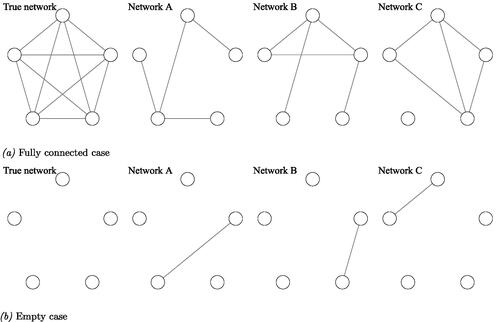
With these assumptions in hand, let us focus on the fully connected network first. Given a sensitivity of 50%, we can expect to pick up, on average, five out of the 10 true edges. Assuming all edges are equal in strength, roughly 50% of the edges will show up in our generated network model at random. Now the question is, if we randomly select three individuals from our homogeneous sample, how much overlap between these three individual network models do we expect to see?

When visually inspecting the individual networks (upper panel Figure 1), one may be tempted to conclude there are plenty of individual differences, as none of the resulting networks look similar to one another. To calculate the overlap between the estimated edges, we could take the number of shared edges between two networks, divided by the number of possible edges ($n(n-1)/2,$ in which n stands for the number of nodes). Multiply by 100 to convert the ratio to a percentage. Using this as a metric to calculate the resemblance between two individual networks, the overlap between network A and B is 20%, the overlap between network A and C is 10%, and between B and C is 40%. If we were to repeat this scenario, on average, we expect to see an overlap of 25% between two randomly selected estimated individual networks, even though the true underlying data generating network structure is exactly the same.

Moving on to the case where our true underlying network is empty, we see even less of an overlap between the generated individual network models (see lower panel Figure 1). Remember, we operate with a specificity of 90%. This implies we have a 10% chance of finding an edge that is absent in reality. The fact that there are 10 potential edges means we expect, on average, one false edge to be included in each estimated network model. Here again, assuming all edges are equal in strength, this erroneous edge can show up anywhere in our network. Once more, let us generate a network for three individuals, see the lower panel Figure 1. When visually inspecting these networks, again, our initial conclusion would be that there is a great deal of variety in the resulting networks. If we were to calculate the overlap between the networks, as we did for our fully connected case, we would now find an overlap between our three networks of 0%. If we were to repeat this scenario, on average, we expect to see an overlap of 10% between any two random individuals.

Analytically, we can derive the probability of obtaining the same network twice in both conditions of our thought experiment (i.e., the true fully connected case and the true empty case) to be: $$\sum _{m=0}^k\left(\begin{array}{c}k\\ m\end{array}\right)p^{2m}{(1-p)}^{\left(\begin{array}{c}n\\ 2\end{array}\right)-2m+k},$$ in which n is the number of nodes, k is the total number of possible edges (i.e., $n(n-1)/2$), and p represents the sensitivity in the fully connected network case and $1-\mathit{specificity}$ in the empty network case. Using this expression, we can calculate that the probability of obtaining the exact same network twice in the thought experiment where the true network is a fully connected, with n = 5 nodes and sensitivity of p = 0.5 to be less than 0.1%. Likewise, we can see that in the case of an empty network with a specificity of 0.9 (i.e., p = 0.1) the probability of obtaining two identical networks is 13.7%.

This thought experiment shows that we can find a great deal of variety in individual networks when visually comparing them, despite our true underlying network model being invariant over individuals. This exposes how prone visual inspection of network models is to error. In addition, often only the number of present edges is taken into account in order to determine overlap between two networks, but if we were to, for example, base the overlap between two networks not only on the estimated edges but also on the absent edges, the overlap between the networks in our fully connected case would rise to 50% and in the empty case to an astonishing 90%. Given our homogeneous sample, another way to increase the estimated overlap between two individual network models could be established by increasing sensitivity. Sensitivity (i.e., the power to detect an existing edge) increases as the number of time points increases. Suppose we increase our sensitivity to 90%. In the case of a fully connected network, this means that if we were to draw two random networks to compare, we would expect an average overlap of 80%, and the chance of two randomly chosen estimated network models to be exactly alike would be 13.7%.

In order to increase power without inflating the Type-I error rate—i.e., increasing sensitivity while keeping specificity high—there is only one solution: we need to collect more data. But how much more data? Much work has been dedicated to identifying the minimum amount of data required when performing ideograph analysis, (e.g., Epskamp et al., 2018c; Lane & Gates, 2017; Mansueto et al., 2022; Nestler & Humberg, 2021),³ however, a considerable variety of results has been reported, likely as a function of simulation and estimation details as well as variation in the network structure simulated from, and were not always viewed in light of perceived heterogeneity. Therefore, it is unclear how much data is needed in order to achieve the preferred sensitivity to make a valid claim about heterogeneity in individual network analysis.

The scenario sketched in our thought experiment is merely a hypothetical one. In reality, we deal with various edge strengths and differences in network structures, such as a more sparse or a more densely connected network structure. There is a delicate interplay between edge weights, network structure, properties of the data (such as sample size and effect size), and the estimation technique used. To shed light on this interplay, we turn to a simulation study to determine the effects of sampling variation on detecting heterogeneity in individual networks under different network structures using three popular estimation techniques.

Beyond thought experiments: Network heterogeneity in estimated network structures

To further illustrate the main point of this paper—be careful with the interpretation of all variability as evidence for individual differences—we conducted a simulation study in which we applied three idiographic network estimation techniques (graphical VAR (graphicalVAR), multilevel VAR (mlVAR) and Group Iterative Multiple Model Estimation (GIMME)) to estimate individual network structures from simulated homogeneous data. This simulation study aims to answer the question to what extent current network-based tools to detect heterogeneity yield valid results to determine the amount of heterogeneity present. Throughout this paper, we have defined the concept of heterogeneity to mean the absence of homogeneity. This is a strong stance on heterogeneity, as the slightest difference is taken as a sign of heterogeneity. Within the network literature, the operationalization of heterogeneity differs. Therefore, it is crucial to have an understanding of different individual network modeling techniques that can be used to operationalize heterogeneity in order to explore if and how these methods account for normal fluctuations within the data. To this end, we provide a brief overview of the most commonly used idiographic network estimation tools.

An overview of idiographic network estimation tools

The most common way to estimate individual networks is with some type of Vector Autoregression (VAR) model. There are two modeling frameworks that extend the VAR model to incorporate both temporal and contemporaneous network structures: the graphical VAR model (GVAR; Epskamp et al., 2018c) and the structural VAR model (SVAR; G. Chen et al., 2011). The GVAR model represents the contemporaneous network using undirected effects, whereas the SVAR model represents the contemporaneous network using direct effects. Several methods exist for estimating model parameters (edge weights) coupled with model structure (presence or absence of edges) for both modeling frameworks and for N = 1 and N > 1 datasets.

In N = 1 settings, the GVAR model can be estimated through iterative regularized estimation by using the multivariate regression with covariance estimation algorithm (MRCE; Abegaz & Wit, 2013; Guo et al., 2010), which is implemented in the R packages graphicalVAR and sparseTSCGM, or it can be estimated through maximum likelihood estimation as implemented in the psychonetrics R package (Epskamp, 2020a, 2020b). The SVAR model can be estimated in the N = 1 setting through model search using generic structural equation modeling software such as the R package lavaan (Rosseel, 2012). In the N > 1 setting, each of the N = 1 methods can be used separately for each individual, a practice investigated in this paper.

In addition to estimating a network model for each individual separately, methods exist that allow one to borrow information across participants. In particular multi-level estimation is often used with the GVAR model by using the two-step multi-level GVAR algorithm as implemented in the R package mlVAR (Epskamp et al., 2018c; 2020), or Bayesian estimation as implemented in Mplus version 8 and higher (Schultzberg & Muthén, 2018). The SVAR model is often estimated in N > 1 settings using GIMME (Gates & Molenaar, 2012), which is implemented in the R package gimme (Lane et al., 2020). For details on the modeling frameworks used in this simulation study and the estimation techniques used, see Supplement A.

In this paper, we focus on three methods for GVAR and SVAR estimation: MRCE using graphicalVAR, two-step multi-level estimation using mlVAR, and Group Iterative Multiple Model Estimation using gimme. We focus on these methods because they have been used for the purpose of estimating individual networks and detecting heterogeneity in existing research (e.g., Beck & Jackson, 2020; Beltz et al., 2016; Bringmann et al., 2013; Reeves & Fisher, 2020; Rodriguez et al., 2022). To simplify the description of results below, we will refer to each of these three methods by referring to their corresponding R packages: graphicalVAR,⁴ mlVAR and GIMME. We expect results from other methods, such as maximum likelihood estimation of N = 1 GVAR models or Bayesian multi-level estimation of N > 1 models, to align, as these methods perform similarly in estimating network structures from data (e.g., Mansueto et al., 2022 shows a strong overlap between the graphicalVAR and psychonetrics packages). In the following sections, we will discuss these three methods, the tools used to detect heterogeneity, and examples of their use in practice for each method separately.

Regularized estimation using graphicalVAR

The graphicalVAR package uses the MRCE algorithm to estimate the GVAR model (Epskamp, 2020a). This algorithm makes use of LASSO regularization (Tibshirani, 1996), which iteratively estimates temporal coefficients (regression weights between t − 1 and t) through regularized regression, and contemporaneous coefficients (partial correlations after controlling for temporal effects) through the graphical LASSO algorithm (Friedman et al., 2008). The algorithm utilizes two LASSO penalty parameters, which are chosen by optimizing the extended BIC (EBIC; J. Chen & Chen, 2008; Abegaz & Wit, 2013; Epskamp et al., 2018c).

It is important to note that as of yet there are no techniques available that are developed specifically to detect heterogeneity using graphicalVAR estimates. The detection of heterogeneity after estimating a GVAR model through graphicalVAR is currently mainly based on (1) differences in network topology, (2) differences in network density, and (3) differences in node connectivity measures (i.e., measures that are often used to assess the relative importance of nodes within the network⁵).

De Vos et al. (2017) can be taken as an example of how visual inspection of individual network models is used to detect heterogeneity. De Vos et al. (2017) estimated individual network models for people diagnosed with Major Depressive Disorder (MDD) and healthy controls. Participants completed a questionnaire assessing seven positive and negative affect items (e.g., “Feeling cheerful” and “Feeling irritated”) three times a day over a period of 30 days. Using visual inspection De Vos et al. concluded that individual networks did not resemble each other in terms of density and topology, taking this as an indication for a strong level of heterogeneity. Fisher et al. (2017) took a somewhat similar approach. The authors estimated individual network models for people with Generalized Anxiety Disorder (GAD) and MDD and for individuals who presented a comorbid clinical picture of both GAD and MDD. Forty participants completed questions on anxiety and depression symptoms (e.g., “Feeling hopeless,” “Loss of interest or pleasure”), positive and negative affect, rumination, behavioral avoidance, and reassurance seeking four times a day for at least 30 days. In addition to examining the network topology, Fisher et al. examined strength centrality. Results showed that node centrality metrics differed strongly between individuals. The authors interpret these differences as an indication for heterogeneity among individuals with GAD, MDD, or a comorbid presentation of GAD and MDD. The two studies described here should be taken merely as examplementary. Given the importance of the question of whether individuals differ from one another (and from the between network structure), more studies with similar interests and set-up can easily be found. For some more recent examples see Jongeneel et al. (2020), Levinson et al. (2022), and Rodriguez et al. (2022).

Multilevel estimation using mlVAR

The second method we discuss is two-step multi-level GVAR estimation using the mlVAR package (Epskamp et al., 2020), which is based on the multi-level VAR models proposed by Bringmann et al. (2013). This package first estimates temporal coefficients by performing a series of multi-level node-wise regressions between time points t − 1 and t. Within-person centering of predictors is used in each of the regressions, and person-wise means are included as between-person predictors, such that within- and between-person effects can be separated (Hamaker & Grasman, 2015). This separation also leads to between-person effects, that are gathered in a between-persons network, which we do not use in the present paper. Next, in a second step, another series of node-wise regressions are performed on the residuals of the first series of node-wise regressions, leading to estimates of contemporaneous networks.

As such, the mlVAR package leads to the estimation of three network structures: (a) a contemporaneous network (per subject and fixed-effect structures over all subjects), (b) a temporal network (per subject and fixed-effect structures over all subjects), (c) a between-subjects network (fixed-effects only). In addition, the standard deviations of random effects across the population on the temporal and contemporaneous network parameters are also returned and can be visualized as networks, leading to two more networks: (d) a temporal network of random effects and (e) a network of the standard deviations from the random effects.

In contrast to fully idiographic N = 1 estimation, for example, by using the graphicalVAR package, multilevel estimation offers a systematic approach to detect heterogeneity. Because of the multilevel structure of the model, one can inspect the network of standard deviations of random effects. These standard deviations show the degree to which network parameters exhibit individual differences. Bringmann et al. (2013) recommend a cutoff of one standard deviation for the resulting edge weights to represent “large inter-individual differences.” This means that every edge with a weight above one standard deviation can be seen as truly heterogeneous. In addition, individual differences can also be observed by visually inspecting personalized networks obtained by adding the fixed and random effects.

Bringmann et al. applied multilevel VAR, on which the mlVAR package is based, to ESM data from 129 participants with depressive symptoms. Participants’ mood was assessed by a questionnaire containing six mood variables (e.g., “Cheerful” and “Fearful”) 10 times a day over a period of 6 days. Bringmann et al. inferred a network of inter-individual differences by examining standard deviations of the random effects. Results indicated a high level of individual variability on the self-loop for worry, as on the self-loops for cheerful, sad, relaxed, and fearful. Furthermore, variability in the relations between cheerful and relaxed, cheerful and sad, and fearful and worry was found, from which the authors concluded that a fair amount of heterogeneity in mood between the participants with depressive symptoms was present. As opposed to tools used to assess heterogeneity for graphical VAR models, the tool used to assess heterogeneity for multilevelVAR—inspecting standard deviations from the random effects—operationalizes heterogeneity in terms of edge weight differences.⁶

Group iterative multiple model estimation (GIMME)

The third method we evaluate is GIMME (Gates & Molenaar, 2012; Lane et al., 2020), as implemented in the gimme package, which is a method for estimating SVAR models in N > 1 datasets (Beltz & Gates, 2017; Lane & Gates, 2017). GIMME makes use of stepwise model search strategies through structural equation models, for example, by utilizing the lavaan package for R. Similar to multilevel modeling, GIMME aims to combine the worlds of nomothetic and idiographic research. However, where multi-level modeling aims to search for quantitative similarity across people (what is the edge-weight?), GIMME aims to search for qualitative similarity across people (which edges are included?). GIMME does this by creating person-specific as well as group-level edges. Group models are estimated by an iterative search procedure that identifies temporal and contemporaneous relationships that would significantly improve model fit for most individuals. After obtaining group-level effects, GIMME will then search for temporal and contemporaneous individual-level effects, continuing this process until an optimal fit is ensured. In addition to individual model output, this leads to a model containing both temporal and contemporaneous group-level edges and temporal and contemporaneous individual-level edges, where the width of the edge corresponds to the number of individuals this edge was estimated for.

The detection of heterogeneity can be executed by inspecting the number of individual paths. Group-level paths reflect homogeneity, as these edges need to be present in at least 75% of the sample, whereas individual paths reflect heterogeneity (Beltz et al., 2016; Beltz & Gates, 2017). This means heterogeneity is operationalized in terms of the number of individual level edges, i.e., edges that did not improve model fit for most individuals but did improve model fit so for specific individuals. Beltz et al. (2016) applied GIMME to data from 25 individuals with personality pathology. Participants were instructed to complete an online survey on related clinically relevant behaviors for 100 consecutive evenings. Sixteen items from the daily surveys concerning behavioral manifestations of personality disorders were used to take four personality facets into account: negative affect, detachment, disinhibition, and hostility. Results revealed some group-level contemporaneous relations indicating some homogeneity, however, weights for these relations differed across participants. In addition, participants showed different relations on the individual level, reflecting heterogeneity.

In sum, several tools are used to assess the amount of heterogeneity for individual network models. However, the question remains how suitable these metrics are to reveal the prevalence of heterogeneity when sampling variation is taken into account. Our ability to disentangle sampling variation from the true effects in our data, i.e., power, is closely related to our ability to detect heterogeneity. A question that arises is whether, with current tools, we have enough power to separate sampling variation from true heterogeneity. To what degree can we be confident that we are looking at heterogeneity and not just normal fluctuations in our data that arise as a function of sampling variance? We investigate this question in simulation studies reported below.

Simulation study

Methods

Network structures

Homogeneous data were generated based on three network structures: a synthetic-data network structure, a more sparse network structure estimated from data of one clinical patient, and a dense network structure estimated from data of multiple patients. We will refer to the first network structure as the synthetic-data network, the second as the case-data network and the third as the Geschwind-data network.⁷

The synthetic-data network structure is a sparse chain graph, e.g., 1–2, 2–3, etc., containing eight nodes, with a network density (the number of present edges divided by the number of possible edges) of 29% for the contemporaneous network and 14% for the temporal network. The average absolute edge weights are $\mathrm{M}=0.34$ and $\mathrm{M}=0.32$ for the contemporaneous and temporal effects respectively. For the data generating PDC and PCC matrices see Supplementary material B.⁸ We included this synthetic-data network model as previous simulation studies have shown that network estimation works well under this structure (Epskamp et al., 2018c). For a graphical representation of the synthetic-data network structure, see Figure 2 panel (a).

Figure 2. Contemporaneous and temporal data generating network models for each individual. The upper panel shows the synthetic-data network with eight nodes simulated to be a chain graph, i.e., 1–2, 2–3, etc. The middle panel shows the case-data network containing seven nodes estimated from clinical data of one subject measured over time. The lower panel shows the Geschwind-data network containing six nodes, estimated from clinical data of multiple subjects. The average contemporaneous and temporal networks are taken as the data-generating network structure for each individual in this study. Edges across networks are scaled to a maximum of 0.69, therewith edges between networks can be visually compared to one another. (a) Synthetic-data network, (b) Case-data network, and (c) Geschwind-data network.

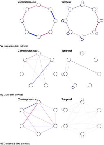
In an attempt to create networks that approximate reality, the other two network structures that were used as data-generating structures are estimated from clinical data. The case-data network is estimated from data of one clinical patient (t = 47) measured over a period of two weeks. The original network was estimated using graphicalVAR and contains seven nodes about the patient’s mood such as “Relaxed,” “Sad” and “Nervous.” For more information on the data, see Epskamp et al. (2018a).⁹ The density of the network is 48% and 10%, with an absolute average edge weight of $\mathrm{M}=0.11$ and $\mathrm{M}=0.16$ for the contemporaneous and temporal networks respectively. For the data generating PDC and PCC matrices, see Supplementary material B; for a graphical representation of the case-data network, see Figure 2, panel (b).

The Geschwind-data network is estimated from data of multiple patients (n = 129) measured over a period of six days (mean $t=60$). For more information on the data set, see Geschwind et al. (2011).¹⁰ The original network was estimated using mlVAR and contains six nodes such as “Cheerful,” “Sad,” and “Relaxed.” For this simulation study, the average contemporaneous and temporal networks were taken as the network structure of one subject. The density of the contemporaneous network and temporal network are 62% and 63%, with an average absolute edge weight of $\mathrm{M}=0.16$ and $\mathrm{M}=0.06$ for the contemporaneous and temporal effects respectively. For the data generating PDC and PCC matrices, see Supplementary material B and for a graphical representation of the Geschwind-data network, see Figure 2, panel (c).

Simulation procedure

Taking these three underlying network structures as the true data generating model for each individual, we simulated homogeneous data in which any apparent individual differences are due to sampling variation. Details on the parameter values under which we simulated can be found in supplementary material B. In addition to network structure, we varied the number of participants, n ∈ {50, 100, 200}, and the number of time points, t ∈ {50, 100, 200, 400}, These time points were chosen to represent plausible values, t ∈ {50, 100}, potentially ideal values, t ∈ {200, 400}, to include scenarios in the simulation where the methods should be expected to function well. We used three different estimation routines (grapicalVAR, mlVAR, and GIMME) to estimate the resulting network models, in total, creating a $3\times 3\times 4$ design. Each condition was repeated 100 times.

In line with common practice, in order to determine the amount of heterogeneity present in estimated network models through graphicalVAR, we evaluated topology of the resulting networks by visually inspecting three randomly chosen estimated network structures. For these individuals, we compared network density, i.e., the number of actual edges divided by the number of possible edges. Furthermore, across the entire sample, we computed the node centrality measure strength for each individual network. Strength centrality is defined as the sum of the edge weights of a given node (in absolute value). For temporal networks, strength is divided into in-strength, the sum of absolute incoming edge-weights, and out-strength, the sum of absolute outgoing edge weights. Centrality measures have been taken as an indication of the importance of individual nodes in a network (Costantini et al., 2015; Opsahl et al., 2010). To determine the amount of resemblance in strength measures across individuals, we correlated the centrality measures for each possible pair of individuals. The distribution of these correlations gives us an idea of the spread of the strength of the association between centrality measures. If centrality measures are in fact a suitable measure for separating sampling variation from heterogeneity, we would expect a narrow distribution peaked around a strong positive correlation, because all samples are drawn from completely homogeneous populations.

For mlVAR estimates, we inspected the distribution of standard deviations of estimated random effects, both for contemporaneous and temporal networks. In line with Bringmann et al. (2013) we used a cutoff score of one standard deviation. Edges from the standard deviation network with a weight above this cutoff are taken to represent” large” heterogeneous effects, whereas edges below this cutoff are taken to be sampling error. In order to compare edge weights estimations from the different network structures, edge weights of the standard deviation networks for both contemporaneous and temporal networks were standardized.

To our knowledge, for GIMME, there is no cutoff or rule of thumb that has been proposed in the literature to determine whether a sample is homogeneous. We suggest taking the percentage of homogeneous edges as an indication of the amount of homogeneity. GIMME provides group-level output in which group-level effects are indicated by black edges, and individual effects are indicted with grey edges (Lane & Gates, 2017). Group level edges are seen as homogeneous, whereas individual level edges are seen as heterogeneous (Beltz & Gates, 2017). To assess the amount of estimated homogeneity, we propose to take the percentage of estimated group level edges, i.e., the number of group level edges divided by the total number of edges estimated in the group level network:¹¹ $$\%\text{of homogeneous edges}=\frac{\#\text{of group level edges}}{\#\text{of group level edges}+\#\text{of individual level edges}}\times 100$$

Data was generated based on the three previously described network structures using the graphicalVARsim function from the graphicalVAR package in R (Epskamp, 2020a) which simulates data from a graphical VAR model. Network models were estimated from the simulated data using the R packages: graphivalVAR (Epskamp, 2020a), mlVAR (Epskamp et al., 2020), and GIMME (Lane et al., 2020). The simulation study was performed in R, version 4.0.2 (R Core Team, 2015). R code for the simulation set-up is included as supplementary materials. In addition, a sensitivity analysis was performed for graphical VAR, multilevel VAR, and GIMME to inspect the resemblance between the data generated networks to the estimated networks. Results for the sensitivity analysis can be found in Appendices B, C & D, for graphical VAR, multilevel VAR, and GIMME, respectively.

Results

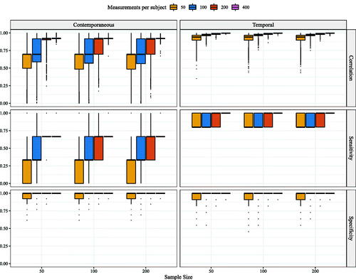
Across all tools, sensitivity was often too low to make valid claims about heterogeneity (for sensitivity analysis of graphical VAR see Figure B1 in Appendix B, for mlVAR see Figure C1 in Appendix C, and for GIMME see Figure D1 in Appendix D).¹² In addition, sensitivity was dependent on network structure for the graphical VAR and the ml VAR method, as well as the estimation technique. Sensitivity was highest when the network structure was sparse (i.e., with relatively few edges) and the edges present were relatively strong as is the case for the synthetic-data network structure. When the network structure was denser, as is the case for the Geschwind-data network, or showed relatively weak edges, sensitivity started to decline. This latter effect was particularly strong when estimating temporal networks using the graphical VAR method, and when estimating contemporaneous networks using GIMME.

To illustrate the lack of sensitivity and its implications for the validity of claims on heterogeneity, we randomly drew three individual networks estimated using the graphical VAR method, from the $5,000$ simulated networks for the synthetic-data network condition (see Figure 3 panel a and c to visually compare the three networks). It is important to note that these networks were chosen to convey how the visual comparison of individual networks can go wrong, especially when sensitivity is low. For t = 50 the individual contemporaneous and temporal networks did not differ much with respect to overall edge weight (Average edge weight and standard deviation for the estimated contemporaneous network model of individual 1: $\mathrm{M}=0.11(\text{SD}=0.09),$ individual 2: $\mathrm{M}=0.15(\text{SD}=0.11),$ and individual 3: $\mathrm{M}=0.14(\text{SD}=0.12);$ Temporal network of individual 1: $\mathrm{M}=0.13(\text{SD}=0.09),$ individual 2: $\mathrm{M}=0(\text{SD}=0),$ and individual 3: $\mathrm{M}=0.16(\text{SD}=0.14)$). However, individual networks differed with respect to network density (network density for estimated contemporaneous networks: 36%, 14%, 46% and temporal network: $44\%,0\%,32\%,$ of individuals 1, 2, and 3 respectively.), and in detected edges. Few similarities could be found in terms of detected edges; in addition, the strength of these edges varied across the three exemplary individual networks.

Figure 3. Output from graphical VAR. Three randomly selected individual networks estimated using the graphical VAR method, generated under the same synthetic-data network structure (for a visualization of the synthetic-data network see Figure 2 panel (b)) for two different time points (t = 50 and t = 400). Panel (a) shows the three individual contemporaneous networks when t = 50, panel (b) for t = 400, panel (c) shows their corresponding temporal networks when t = 50, and panel (d) for t = 400. (a) Contemporaneous networks for individual 1, 2, and 3 when t = 50, (b) Contemporaneous networks for individual 1, 2, and 3 when t = 400, (c) Temporal networks for individual 1, 2, and 3 when t = 50, and (d) Temporal networks for individual 1, 2, and. 3 when t = 400.

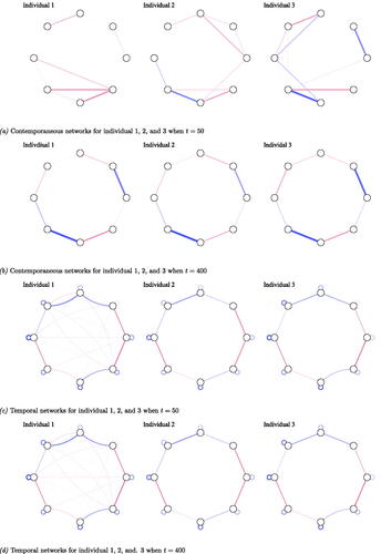
Perceived heterogeneity vanished when visually inspecting the estimated network structures using graphical VAR when t = 400, see panels (b) and (d) in Figure 3. When visually inspecting the individual contemporaneous networks, the networks showed significant resemblance. Note that sensitivity is high for the contemporaneous networks; all seven data generating edges were estimated for each of the individual networks. However, in terms of network density, we still found notable differences. For the contemporaneous networks density differed (32%, 43%, 29%, for t = 400 for individuals 1, 2, and 3 respectively), as networks A and B showed a few weak erroneous edges. These edges can be disregarded in terms of edge weight in comparison to the other edges present. In terms of overall edge weight we found slight differences (average edge weight and standard deviation for the estimated contemporaneous network model of individual 1: $\mathrm{M}=0.18(\text{SD}=0.14),$ individual 2: $\mathrm{M}=0.18(\text{SD}=0.14),$ and individual 3: $\mathrm{M}=0.22(\text{SD}=0.12)$).

Although sensitivity for temporal networks as estimated with graphical VAR was high at t = 400, the exemplary temporal networks of individual 1, 2, and 3 showed a larger range of network density than for their contemporaneous networks (network density of 63%, 57%, 37%, for the estimated temporal networks of individual 1, 2 and 3 respectively). In terms of overall absolute edge weight, we found small differences (temporal network individual 1: $\mathrm{M}=0.15(\text{SD}=0.13),$ individual 2: $\mathrm{M}=0.14(\text{SD}=0.13),$ individual 3: $\mathrm{M}=0.20(\text{SD}=0.13)$). Heterogeneity in terms of estimated edges, network density, and edge weights was more pronounced for the case-data and the Geschwind-data network structures. Examples of three networks estimated under the case-data and the Geschwind-data network structure can be found in Figures A1 and A2 in Appendix A.

Moving forward, we investigated the use of centrality measures as an indication of individual differences between networks. For the entire sample, based on each individual network as estimated with the graphical VAR method, node centrality strength was computed. For contemporaneous networks, we computed one measure: strength (the sum of all absolute edge weights connected to the node), for temporal networks, this measure is divided in in-strength (the sum of all absolute incoming edge-weights) and out-strength (the sum of all absolute outgoing edge weights). For all possible pairs of individual networks within the sample, the strength estimates were correlated in order to give an indication of the resemblance in strength centrality. Figure 4 shows the distributions of the correlation of these strength measures for the entire sample. Regardless of network structure, strength measures correlated more with one another for contemporaneous and temporal networks as the number of time points increased. Furthermore, strength measures showed a higher correlation for contemporaneous networks than for temporal networks. For all three network structures, the correlation of strength measures for the contemporaneous network are somewhat similar from roughly t = 200 onward.

Figure 4. Correlations between node strength centrality calculated from individual networks estimated with graphical VAR. For the contemporaneous network, the correlation between strength centrality is depicted. For temporal networks, the correlations for two strength measures were computed: in-strength and out-strength. Correlations between strength measures of contemporaneous networks are highest for networks estimated under the Geschwind-data structure, while the in- and out-strength correlations are highest for networks generated under the synthetic-data structure.

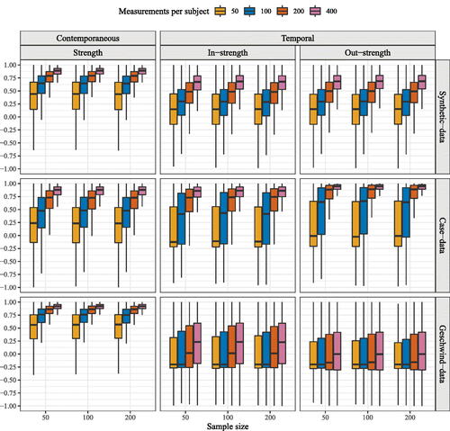
The median correlation for in- and out-strength for the Geschwind-data network remained low in all cases, in-strength: $\mathrm{r}=0.23,$ out-strength: $\mathrm{r}=-0.002.$ For the case-data network the median correlation for in-strength and out-strength increased from $r=-0.13$ and $r=-0.009,$ to r = 0.86 and r = 0.94 respectively. For the synthetic-data network the median correlation for in- and out-strength increased from r = 5.14 and r = 0.15 to r = 0.67 and r = 0.63. Surprisingly, in- and out- strength correlation increased most for the case-data network as opposed to the synthetic-data network.

It is important to note here that the correlation between node strengths, although regularly used in the literature, is a problematic measure of similarity (Borsboom et al., 2017; Forbes et al., 2017a). This is because, in general, weak correlations may be the result of low variance in estimated edge weights (i.e., a situation in which all edge weights are approximately the same). If the variance in individual centrality measures is low this can lead to very weak correlations (around zero) between two individual centrality measures, even when measures are similar. This means a high correlation could be an indication of similarity in strength centrality, while a weak correlation may also be an indication of similarity—making the interpretation of correlations asymmetric and less intuitive. In this particular case, however, weak correlations did not result because of a lack of variance, but rather because of a lack of a linear relation between individuals’ centrality measures. Therefore, here we may safely interpret weak correlations as an indication of a lack of resemblance.

For mlVAR estimation results, we inspected the standard deviation of random effects for the contemporaneous and temporal effects. We took a cutoff of one standard deviation for the edge weights to determine whether population heterogeneity was present. In order to compare the edge weights of the different network structures and their standard deviations, edge weights were standardized. Standardized density distributions of the standard deviation of random effects for the contemporaneous and temporal effects can be found in Figure 5.

Figure 5. Density distribution of standardized edge weights for standard deviations of random effects for the multilevel VAR model. The vertical black dotted line represents the recommended cutoff of one standard deviation. Edges above or below these cutoff’s are seen as truly heterogeneous.

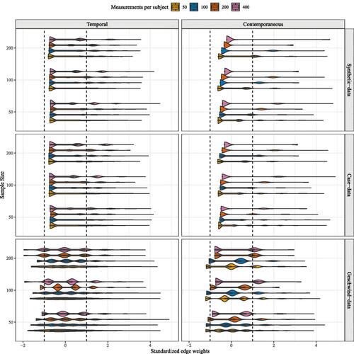
For contemporaneous network structures, the estimation of large heterogeneous effects was limited with relatively small sample sizes n = 50 and t = 50. For each of the three data generating network structures, no heterogeneous edges were detected when the number of individuals increased to n = 200 and the number of time points per subject to t = 400. For all temporal network structures with n = 50, the estimation of heterogeneous edges was limited. Fewer differences were detected for the synthetic-data network structure and the case-data network structure than under a Geschwind-data network structure. When increasing time points to t = 200 per individual, even less heterogeneity was detected.

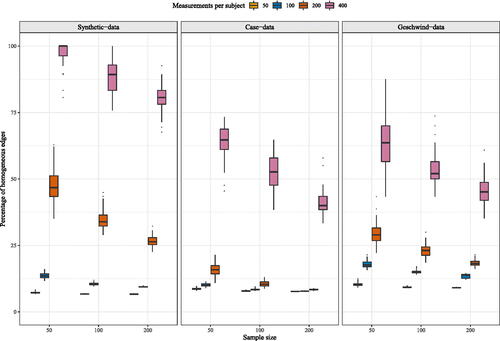
In contrast to mlVAR, to the best of our knowledge, for GIMME there has been no cutoff recommended in the literature. We decided to inspect the percentage of homogeneous edges and take this as an indication of the amount of heterogeneity present, see Figure 6. The percentage of homogeneous edges was $7\%(\text{SD}=0.33\%),9\%(\text{SD}=0.33\%),10\%(\text{SD}=0.64\%)$ for n = 50 and t = 50 for the synthetic-data, case-data and Geschwind-data network structures respectively. This percentage increased as the number of time points increased. When t = 400 the median percentage of homogeneous edges was $97\%(\text{SD}=4.45\%),64\%(\text{SD}=5.48\%),64\%(\text{SD}=8.63\%)$ for synthetic-data, case-data and Geschwind-data network structures. Interestingly, we found that the percentage of homogeneous edges detected decreased as the number of participants increased. The same pattern was found for a larger synthetic-data network structure, see Figure S10 in supplementary materials B.

Figure 6. Percentage of homogeneous edges as estimated through GIMME for the synthetic-data, case-data, and Geschwind-data network structures.

Discussion

The present paper aimed to expose effects of sampling variation and power limitations in the investigation of heterogeneity in idiographic network models. We have shown that, even if the underlying network model is invariant across individuals, limitations regarding specificity and sensitivity can impose a great deal of variety in individual network structures estimated from the data, especially when the number of time points is small. In a simulation study, we evaluated four different network tools for assessing heterogeneity: visual inspection, comparing centrality measures, inspecting random effect standard deviations, and applications of GIMME. Results showed that low statistical power places considerable limits on the validity of conclusions regarding heterogeneity for all tools. At low sample sizes, an applied researcher is likely to erroneously conclude that a sample is heterogeneous even if it is in fact, homogeneous. Under the right circumstances (high sample size and favorable generating network structures), inspecting the standard deviation of random effect using multilevel VAR modeling and GIMME proved most suited for detecting heterogeneity, but these circumstances are currently not realized in the great majority of designs in many relevant fields, such as psychopathology research.

Many lower-powered analyses versus one high-powered analysis

When comparing idiographic network models, an important pitfall lies in the tendency to interpret all variability in resulting networks as heterogeneity between people, while some of this variability is the result of fluctuations in the data created by noise—e.g., sampling variation. Combining sampling variation with overall conservative estimation procedures (high specificity and lower sensitivity at low sample sizes) will inevitably lead to a mismatch in the presence and absence of estimated edges in addition to varying edge weights across individuals. Of course, the most straightforward way to combat these problems is to collect more data in an effort to increase statistical power without inflating the Type I error (i.e., increasing sensitivity while keeping specificity high).

Importantly, the number of time points needed to estimate robust idiographic network models is dependent on the network structure (e.g., a more sparse or dense network structure) and the estimation technique used. However, we found that even when we simulated under ideal conditions—a sparse network structure with strong edges—at least 200 time points per individual may be needed to obtain network structures that are sufficiently robust to support comparisons between individuals. The amount of time series data needed quickly adds up if the network structure is less than optimal, such as when one is dealing with a sparse or dense structure with weak edges. In these cases, the number of time points one needs per individual may exceed 400. This amount of data is often not realized in current research practice typical applications in, e.g., psychopathology research. Although some cases have been known to feature sufficiently intense measurement schemes in this respect (Kossakowski et al., 2017), one rarely encounters time series of this length in, for instance, ESM designs.

In practice, we may see only about 60 observations per individual (e.g., Beck & Jackson, 2020; Jongeneel et al., 2020; Rodriguez et al., 2022), which might seem like a large amount of data given the difficulty of collecting it, but this may not be enough to estimate a robust individual network. If longer time series cannot be obtained per individual, then the only other solution is to step down from fully idiographic research (estimate one model per person) and instead use an analysis strategy that borrows information from other participants (e.g., multi-level modeling or GIMME). This may then lead to performing one well-powered analysis rather than a sequence of lower-powered analyses at the idiographic level. Such methods performed best in our simulations as well. However, both methods still showed a great deal of illusionary heterogeneity (few common edges in GIMME and relative large random effect sizes in multi-level VAR modeling) and come with their own disadvantages, such as the assumption of heterogeneity, or in the case of multi-level modeling, pulling individual estimations toward the group mean (Bringmann et al., 2013).

Comparing centrality across individuals

There is an ongoing debate on the use and interpretation of centrality measures in network analysis (Bringmann et al., 2019; Dablander & Hinne, 2018; Hallquist et al., 2021). Our results add to the discussion by showing that if one wants to use centrality measures as a way to determine heterogeneity, one should proceed with caution. Here we share four considerations to illustrate this. First, as we showed in our simulation study, it is possible to find negative correlations between estimated strength measures for two generated networks with the same true underlying network structure when the number of observations is less than t = 100 per individual. Second, although adding data leads to a stronger correlation of strength centrality measures between individuals in most settings, we showed that it is possible that the correlation between centrality coefficients is low even with a large number of data points per individual (t > 200). Third, while weak correlations between strength centrality can be the result of a lack of overlap between two networks, this need not be the case because weak correlations between strength centrality can also be the result of low variance. While strong correlations between centrality measures are an indication of similarities between strength centrality, weak correlations do not necessarily have to be an indication of dissimilarity in strength centrality, making the interpretation of correlations between strength centrality counterintuitive; this warrants even more caution in the interpretation of these correlations. Fourth and last, the supposed difference in centrality measures could be due to sampling variation; hence, in the absence of systematic ways to statistically assess the correlation between centrality measures, it does not provide any way to differentiate between real heterogeneity and random fluctuations in the data.

Importantly, this does not mean that centrality coefficients cannot be used to study network topology or individual differences therein. Instead, it means that, just like with any other statistic, inspecting centrality estimates must always be assisted by assessments of precision and robustness (e.g., confidence or credibility intervals and other functions of sampling distributions). Such assessments have now become standard in cross-sectional network analysis (Epskamp et al., 2018b). Future research should investigate extending such methods for application to time-series data. Until suitable measures of precision have become available, the use of visual inspection of differences in centrality measures to detect heterogeneity in network analysis must be considered questionable.

Network heterogeneity and replicability

The discussion of heterogeneity in idiographic network models both resembles and mirrors the discussion on network replicability in cross-sectional network studies (Borsboom et al., 2017; Forbes et al., 2017a). In cross-sectional network analysis, it has been recognized that there may be a great deal of sampling variation in the estimated network structures, which, combined with conservative estimation methods, may by itself lead to differences in estimated network models (Fried et al., 2021). In addition, it has been recognized that fluctuations in centrality measures may be due to sampling variation even at high sample sizes, depending on the generating network structure and the centrality measure chosen (Epskamp et al., 2018b). To this end, data-driven sampling methods or more sophisticated statistical methods are routinely used together with presented results to assess accuracy and stability in a sample as well as to statistically compare network structures of different samples (Epskamp et al., 2018b; Van Borkulo et al., 2017; Williams et al., 2020), as presumably, both sampling variation and heterogeneity lead to differences in estimated network structures.

In the literature on cross-sectional network models, differences between estimated network structures are sometimes highlighted as evidence for limited replicability of network models (Forbes et al., 2017a; 2017b). However, these differences should be expected to arise partly due to the expected replicability of a method given its sensitivity and specificity (Williams et al., 2020). When studying genuine heterogeneity over different samples used for network analysis, assessments of heterogeneity cannot be assessed without taking sampling variation into account (Isvoranu et al., 2020). This also holds true for network models (or any other statistical model) estimated from time-series data. Of note, even though we simulated 400 data points as our largest sample size, such a sample size is not deemed very large when estimating a cross-sectional network of, for example, 10 nodes (featuring 45 parameters). Time-series data features auto-correlations due to temporal ordering of the data, which both require more parameters to be estimated (145 in total for a graphical VAR model) and leads to effectively less information per observation. Both factors lead to a lower expected “replicability” of the network structures, which is highlighted in our simulation results.

Limitations and future directions

At least two limitations of the current simulations need to be addressed here. First, although GIMME performed well with sufficient amounts of data, there is reason to believe the current simulation setup might put GIMME at a disadvantage. In our simulation study, we generated data based on graphicalVAR models, GIMME, however, operates under a structural VAR (SVAR) model. Running simulation conditions using a SVAR model underlying the data yielded similar results as for the GVAR models. However, our simulation study highlighted the influence of the network structure on the results. As GIMME was evaluated under just one SVAR structure, generalizations must be made cautiously. Thus, the present findings speak to the effectiveness of using GIMME when assessing heterogeneity in data that arise from a given VAR model as specified in this paper but have less bearing on the general quality of GIMME as a statistical procedure operating within its own data space. Second, although the most common way to estimate individual networks is by using some type of VAR model, it should be noted that many more estimation procedures exist, for example, based on other types of autoregressive (AR) models than the VAR model, such as AR Moving Average (ARMA) or integrated ARMA (ARIMA) (Box et al., 1970; for an overview of these techniques see: Hamaker and Dolan (2009)). However, we found that most of the network model papers focusing on the detection of heterogeneity made use of the techniques evaluated in this paper.

We conclude by highlighting future avenues for the comparison of individual networks regarding heterogeneity. The current paper has shown that several techniques used to compare individual network models are of limited usefulness in disentangling true heterogeneity from noise. Therefore, there is a pressing need for the development of tools that can do so effectively. A first possible route for future research is to rely more on hierarchical or multi-level models in which heterogeneity across individuals can explicitly be included in the model as random effects and tested to feature non-zero variance. Currently, the mlVAR package, which can be used for multi-level graphical VAR estimation, does not allow for this comparison. An alternative is to use the Dynamical Structural Equation Modeling (DSEM) module in MPlus (Schultzberg & Muthén, 2018), which allows for estimating multi-level VAR models, but with marginal correlations rather than partial correlations between innovation terms. This will allow for assessing random effects on temporal structures but not on contemporaneous partial correlation networks. A second option is to extend data-driven methods used to investigate differences in cross-sectional networks to results from time-series models (Van Borkulo et al., 2017). A problematic aspect here, however, is that resampling techniques cannot readily be applied as the temporal ordering of the data plays an important role in the analysis as well. Finally, promising Bayesian methods have been developed to assess not only evidence for differences but also evidence for the similarity between different samples (Williams et al., 2020). Such methods could perhaps also be expanded for time-series analysis.

Conclusion

In the quest to address the individual within psychology, some concerns arising from the use of these individual models are in danger of being overlooked, including common statistical problems that arise due to sampling variation. Although research within the field of individual network analysis is promising, it is vital to recognize the core principle of statistical analysis: accounting for the uncertainty that arises as a result of sampling variation. Sampling variation alone can lead to striking differences (illusory heterogeneity) in estimated models from different subjects, even if these subjects are identical (fully homogeneous). This article aimed to function as a wake-up call, addressing some of the concerns regarding analyzing the individual and calls for caution in the use and interpretation of these new time series techniques when making claims about heterogeneity.

Article information

Conflict of interest disclosures: Each author signed a form for disclosure of potential conflicts of interest. No authors reported any financial or other conflicts of interest in relation to the work described.

Ethical principles: The authors affirm having followed professional ethical guidelines in preparing this work. These guidelines include obtaining informed consent from human participants, maintaining ethical treatment and respect for the rights of human or animal participants, and ensuring the privacy of participants and their data, such as ensuring that individual participants cannot be identified in reported results or from publicly available original or archival data.

Funding: This work was supported by the NWO Research Talent Grant no. 406-18-532 awarded to R. H. A. Hoekstra, NWO Veni Grant no. 016-195-261 awarded to S. Epskamp and ERC Consolidator Grant no. 64209 and NWO Vici Grant VI.C.181.029 awarded to D. Borsboom.

Role of the funders/sponsors: None of the funders or sponsors of this research had any role in the design and conduct of the study; collection, management, analysis, and interpretation of data; preparation, review, or approval of the manuscript; or decision to submit the manuscript for publication.

Acknowledgments: The authors would like to thank Nathan Evans for lending a helping hand in the simulation study procedures. In addition, the authors would like to thank Julius Pfadt, the Associate Editor Douglas Steinley, and the anonymous reviewers for their comments on prior versions of this manuscript. The ideas and opinions expressed herein are those of the authors alone, and endorsement by the authors’ institution or the NWO and ERC is not intended and should not be inferred.

Notes

1 Interestingly, the network paradigm was also foreshadowed by Molenaar’s work, as he was the first to identify the relation between the Ising model from statistical mechanics—a model very similar to the GGM but applied to dichotomous data—and the Rasch model from Item Response Theory (Molenaar, 2003, p. 82).

2 For simplicity, we will use undirected contemporaneous networks and ignore temporal effects by assuming temporal networks are empty. The thought experiment could easily be extended to temporal networks as well, as the same logic holds.

3 The work of Epskamp et al. (2018c) shows t = 100 is sufficient when performing a grpahicalVAR analysis, while the work of Mansueto et al. (2022) shows sufficient sensitivity when t = 500. In addition, Lane and Gates (2017), show t > 60 is suitable for GIMME to pick up small to moderate effects while the work of Nestler and Humberg (2021) shows t > 100 for GIMME to perform well.

4 GraphicalVAR therefore refers to the MRCE method implemented in the graphicalVAR R package, not to the GVAR modeling framework, which can also be estimated using other methods.

5 For an overview of connectivity measures often used in psychological networks see Costantini et al. (2015) and Robinaugh et al. (2016).

6 Which is indirectly related to network topology and density.

7 As these data generating matrixes are based on GVAR models, while GIMME operates under a SVAR model, we have included an additional SVAR network structure and preformed the simulation set up as described in this section. For more details on the SVAR network structure, simulaiton set up and results see Supplement B.

8 In addition to a synthetic-data network structure with 8 nodes, a sparse chain graph containing 16 nodes was generated in similar fashion to inspect the effect of the size of the network. Results for this large network structure can be found in the Supplementary Material B.

9 The dataset used for generating the network used in the current simulation study can be found in the supplementary materials of Epskamp et al. (2018a).

10 The dataset used for generating the network used in the current simulation study can be found in the supplementary materials of Bringmann et al. (2013).

11 It is important to note that individual effects can be both contemporaneous and temporal. If an individual effect was estimated both as contemporaneous for some individuals and temporal for others, this was taken to mean there is some level of heterogeneity, and both edges added up to the total number of individual edges.

12 Sensitivity analysis for GIMME was infeasible for the original three data generating network structures as the data generating model for a GVAR model does not directly correspond to one SVAR model (the modeling framework used by GIMME to estimate networks). However, one SVAR does directly correspond to a unique GVAR model. Therefore, a SVAR data generating network is added to the simulation study, see Supplement B for further details on the data generating network structure and the full simulation study results.

 

Appendix A

Visual inspection networks

To further illustrate the lack of sensitivity and its implications for the validity of claims on heterogeneity, we randomly drew three individual networks from the $5,000$ simulated networks for the case-data and Geschwind-data network conditions (see panel (a) and (c) Figures A1 and A2) to visually compare the three networks for t = 50. Where in the synthetic-data condition, the perceived heterogeneity vanished when visually inspecting the estimated network structures for t = 400 (see panel (b) and (d) Figure 3), there still seemed to be considerable heterogeneity present when visually inspecting the estimated network structures for the case-data and Geschwind-data network structures when t = 400 (see Figures A1 and A2 panel b and d).

Figure A1. Output from graphical VAR. Three individual networks (contemporaneous and temporal) were generated under the same case-data network structure. Panel (a) shows the contemporaneous networks for t = 50, (b) for t = 400, (c) their corresponding temporal networks with t = 50, and (d) for t = 400. (a) Contemporaneous network for individual 1, 2, and 3 when t = 50, (b) Contemporaneous network for individual 1, 2, and 3 when t = 400, (c) Temporal network for individual 1, 2, and 3 when t = 50, and (d) Temporal network for individual 1, 2, and 3 when t = 400.

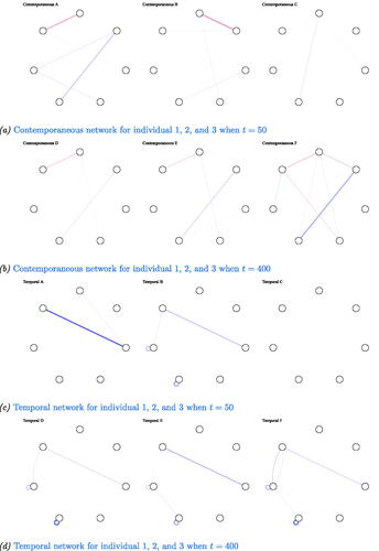
Figure A2. Output from Graphical VAR. Three individual networks (contemporaneous and temporal) were generated under the same Geschwind-data network structure. Panel (a) shows the contemporaneous networks for t = 50, (b) for t = 400, (c) their corresponding temporal networks with t = 50, and (d) for t = 400. (a) Contemporaneous network for individual 1, 2, and 3 when t = 50, (b) Contemporaneous network for individual 1, 2, and 3 when t = 400, (c) Temporal network for individual 1, 2, and 3 when t = 50, and (d) Temporal network for individual 1, 2, and 3 when t = 400.

 

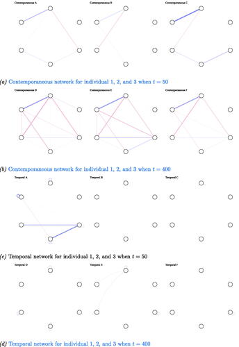
Appendix B

Sensitivity analysis graphical VAR

Figure B1. Sensitivity results for graphical VAR. Correlation, sensitivity, and specificity for contemporaneous and temporal individual networks for synthetic-data, case-data, and Geschwind-data network structures.

 

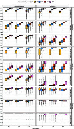
Appendix C

Sensitivity analysis multilevel VAR

Figure C1. Sensitivity results for multilevel VAR. Correlation, sensitivity, and specificity are depicted for contemporaneous and temporal individual networks for synthetic-data, case-data, and Geschwind-data network structures. In line with previous simulation study results, sensitivity is 100% and specificity 0% as a result of all edges being estimated (see Epskamp et al. (2018a). Therewith, the correlation between the data generating network model and the estimated network model is a better indication of the power of the estimation technique.

 

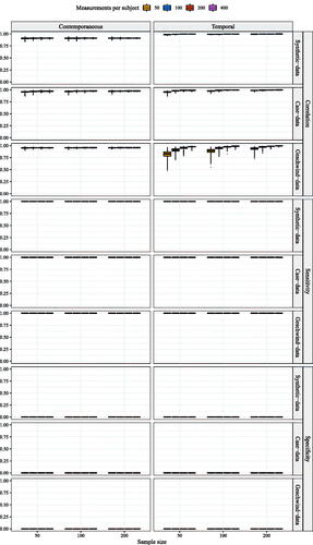
Appendix D

Sensitivity analysis GIMME

Figure D1. Sensitivity results for GIMME. Correlation, sensitivity, and specificity are depicted for contemporaneous and temporal individual networks as simulated under a structural VAR network and estimated using GIMME. More details on the simulation procedure and parameter values of the data generating network structure can be found in supplement B. Important to note here is that the diagonal of the temporal matrix is taken into account when computing the sensitivity to make the comparison between sensitivity results for GIMME, graphicalVAR, and mlVAR more straightforward.

References

- Abegaz, F., & Wit, E. (2013). Sparse time series chain graphical models for reconstructing genetic networks. Biostatistics (Oxford, England), 14(3), 586–599.
- Beck, E. D., & Jackson, J. J. (2020). Consistency and change in idiographic personality: A longitudinal ESM network study. Journal of Personality and Social Psychology, 118(5), 1080–1100.
- Beltz, A. M., & Gates, K. M. (2017). Network mapping with GIMME. Multivariate Behavioral Research, 52(6), 789–804.
- Beltz, A. M., Wright, A. G. C., Sprague, B. N., & Molenaar, P. C. M. (2016). Bridging the nomothetic and idiographic approaches to the analysis of clinical data. Assessment, 23(4), 447–458. https://doi.org/10.1177/1073191116648209
- Borsboom, D. (2017). A network theory of mental disorders. World Psychiatry, 16(1), 5–13. https://doi.org/10.1002/wps.20375
- Borsboom, D., & Cramer, A. O. J. (2013). Network analysis: An integrative approach to the structure of psychopathology. Annual Review of Clinical Psychology, 9(1), 91–121. https://doi.org/10.1146/annurev-clinpsy-050212-185608
- Borsboom, D., Fried, E. I., Epskamp, S., Waldorp, L. J., Borkulo, C. D., van, van der Maas, H. L., & Cramer, A. O. (2017). False alarm? A comprehensive reanalysis of “evidence that psychopathology symptom networks have limited replicability” by Forbes, Wright, Markon, and Krueger (2017). Journal of Abnormal Psychology, 126(7), 989–999. https://doi.org/10.1037/abn0000306
- Borsboom, D., Mellenbergh, G. J., & Van Heerden, J. (2003). The theoretical status of latent variables. Psychological Review, 110(2), 203–219.
- Bos, E. H., & Wanders, R. B. (2016). Group-level symptom networks in depression. JAMA Psychiatry, 73(4), 411. https://doi.org/10.1001/jamapsychiatry.2015.3103
- Box, G. E., Jenkins, G. M., Reinsel, G. C., & Ljung, G. M. (1970). Time series analysis: Forecasting and control. Holden-Day.
- Bringmann, L. F., Elmer, T., Epskamp, S., Krause, R. W., Schoch, D., Wichers, M., Wigman, J. T. W., & Snippe, E. (2019). What do centrality measures measure in psychological networks? Journal of Abnormal Psychology, 128(8), 892–903. https://doi.org/10.1037/abn0000446
- Bringmann, L. F., Vissers, N., Wichers, M., Geschwind, N., Kuppens, P., Peeters, F., Borsboom, D., & Tuerlinckx, F. (2013). A network approach to psychopathology: New insights into clinical longitudinal data. PLoS One, 8(4), e60188. https://doi.org/10.1371/journal.pone.0060188
- Burger, J., Veen, D. C. V. D., Robinaugh, D. J., Quax, R., Riese, H., Schoevers, R. A., & Epskamp, S. (2020). Bridging the gap between complexity science and clinical practice by formalizing idiographic theories: A computational model of functional analysis. BMC Medicine, 18(1), 99–18. https://doi.org/10.1186/s12916-020-01558-1
- Chen, J., & Chen, Z. (2008). Extended Bayesian information criteria for model selection with large model spaces. Biometrika, 95(3), 759–771. https://doi.org/10.1093/biomet/asn034
- Chen, G., Glen, D. R., Saad, Z. S., Hamilton, J. P., Thomason, M. E., Gotlib, I. H., & Cox, R. W. (2011). Vector autoregression, structural equation modeling, and their synthesis in neuroimaging data analysis. Computers in Biology and Medicine, 41(12), 1142–1155.
- R Core Team. (2015). R: A language and environment for statistical computing 55. R Development Core Team, 55, 275–286.
- Costantini, G., Epskamp, S., Borsboom, D., Perugini, M., Mõttus, R., Waldorp, L. J., & Cramer, A. O. (2015). State of the aRt personality research: A tutorial on network analysis of personality data in R. Journal of Research in Personality, 54, 13–29. https://doi.org/10.1016/j.jrp.2014.07.003
- Cramer, A. O., Waldorp, L. J., Van Der Maas, H. L., & Borsboom, D. (2010). Comorbidity: A network perspective. The Behavioral and Brain Sciences, 33(2-3), 137–193. https://doi.org/10.1017/S0140525X09991567
- Dablander, F., & Hinne, M. (2018). Centrality measures as a proxy for causal influence? A cautionary tale. Preprint Downloaded from PsyArXiv.
- De Vos, S., Wardenaar, K. J., Bos, E. H., Wit, E. C., Bouwmans, M. E., & De Jonge, P. (2017). An investigation of emotion dynamics in major depressive disorder patients and healthy persons using sparse longitudinal networks. PLoS One, 12(6), e0178586.
- Epskamp, S. (2020b). Psychometric network models from time-series and panel data. Psychometrika, 85(1), 206–231. https://doi.org/10.1007/s11336-020-09697-3
- Epskamp, S., Borkulo, C. D., van, Veen, D. C., van der, Servaas, M. N., Isvoranu, A. M., Riese, H., & Cramer, A. O. (2018a). Personalized network modeling in psychopathology: The importance of contemporaneous and temporal Connections. Clinical Psychological Science, 6(3), 416–427.
- Epskamp, S., Borsboom, D., & Fried, E. I. (2018b). Estimating psychological networks and their accuracy: A tutorial paper. Behavior Research Methods, 50(1), 195–212.
- Epskamp, S., Maris, G. K. J., Waldorp, L. J., & Borsboom, D. (2016). Network psychometrics. In P. Irwing, D. Hughes, & T. E. Booth (Eds.), Handbook of psychometrics. Wiley.
- Epskamp, S., Waldorp, L. J., Mõttus, R., & Borsboom, D. (2018c). The Gaussian graphical model in cross-sectional and time-series data. Multivariate Behavioral Research, 53(4), 453–480.
- Epskamp, S. (2020a). Graphicalvar: Graphical var for experience sampling data [Computer software manual]. Retrieved from https://cran.r-project.org/package=graphicalVAR
- Epskamp, S., Deserno, M. K., Bringmann, L. F. (2020). mlvar: Multi-level vector autoregression [Computer software manual]. Retrieved from https://cran.r-project.org/web/packages/mlVAR/index.html
- Fisher, A. J., Medaglia, J. D., & Jeronimus, B. F. (2018). Lack of group-to-individual generalizability is a threat to human subjects research. Proceedings of the National Academy of Sciences, 115(27), E6106–E6115. https://doi.org/10.1073/pnas.1711978115
- Fisher, A. J., Reeves, J. W., Lawyer, G., Medaglia, J. D., & Rubel, J. A. (2017). Exploring the idiographic dynamics of mood and anxiety via network analysis. Journal of Abnormal Psychology, 126(8), 1044–1056.
- Forbes, M. K., Wright, A. G., Markon, K. E., & Krueger, R. F. (2017a). Evidence that psychopathology symptom networks have limited replicability. Journal of Abnormal Psychology, 126(7), 969–988. https://doi.org/10.1037/abn0000276
- Forbes, M. K., Wright, A. G., Markon, K. E., & Krueger, R. F. (2017b). Further evidence that psychopathology networks have limited replicability and utility: Response to Borsboom et al.(2017) and Steinley et al.(2017). Journal of Abnormal Psychology, 126(7), 1011–1016.
- Fried, E. I., van Borkulo, C. D., & Epskamp, S. (2021). On the importance of estimating parameter uncertainty in network psychometrics: A response to Forbes et al.(2019). Multivariate behavioral research, 56(2), 243–248.
- Fried, E. I., Borkulo, C. D., van, Cramer, A. O., Boschloo, L., Schoevers, R. A., & Borsboom, D. (2017). Mental disorders as networks of problems: A review of recent insights. Social Psychiatry and Psychiatric Epidemiology, 52(1), 1–10.
- Friedman, J., Hastie, T., & Tibshirani, R. (2008). Sparse inverse covariance estimation with the graphical lasso. Biostatistics (Oxford, England), 9(3), 432–441.
- Gates, K. M., & Molenaar, P. C. M. (2012). Group search algorithm recovers effective connectivity maps for individuals in homogeneous and heterogeneous samples. NeuroImage, 63(1), 310–319.
- Geschwind, N., Peeters, F., Drukker, M., van Os, J., & Wichers, M. (2011). Mindfulness training increases momentary positive emotions and reward experience in adults vulnerable to depression: A randomized controlled trial. Journal of Consulting and Clinical Psychology, 79(5), 618–628. https://doi.org/10.1037/a0024595
- Granger, C. J. W. (1969). Investigating causal relations by econometric models and cross-spectral methods. Econometrica, 37(3), 424–438. https://doi.org/10.2307/1912791
- Guo, J., James, G., Levina, E., Michailidis, G., & Zhu, J. (2010). Principal component analysis with sparse fused loadings. Journal of Computational and Graphical Statistics, 19(4), 930–946. https://doi.org/10.1198/jcgs.2010.08127
- Hallquist, M. N., Wright, A. G., & Molenaar, P. C. (2021). Problems with centrality measures in psychopathology symptom networks: Why network psychometrics cannot escape psychometric theory. Multivariate Behavioral Research, 56(2), 199–223.
- Hamaker, E. L., & Dolan, C. V. (2009). Idiographic data analysis: Quantitative methods—from simple to advanced. In J. Valsiner, P. C. M. Molenaar, M. C. D. P. Lyra, & N. Chaudhary (Eds.), Dynamic process methodology in the social and developmental sciences (pp. 191–216). Springer–Verlag.
- Hamaker, E. L., Dolan, C. V., & Molenaar, P. C. (2005). Statistical modeling of the individual: Rationale and application of multivariate stationary time series analysis. Multivariate Behavioral Research, 40(2), 207–233. https://doi.org/10.1207/s15327906mbr4002_3
- Hamaker, E. L., & Grasman, R. P. P. P. (2015). To center or not to center? Investigating inertia with a multilevel autoregressive model. Frontiers in Psychology, 5, 1–5.
- Isvoranu, A. M., Epskamp, S., Cheung, M. W. L. (2020). Network models of post-traumatic stress disorder: A meta-analysis. Retrieved from https://psyarxiv.com/8k4u6
- Jongeneel, A., Aalbers, G., Bell, I., Fried, E. I., Delespaul, P., Riper, H., van der Gaag, M., & van den Berg, D. (2020). A time-series network approach to auditory verbal hallucinations: Examining dynamic interactions using experience sampling methodology. Schizophrenia Research, 215, 148–156. https://doi.org/10.1016/j.schres.2019.10.055
- Kievit, R. A., Frankenhuis, W. E., Waldorp, L. J., & Borsboom, D. (2013). Simpson’s paradox in psychological science: A practical guide. Frontiers in Psychology, 4, 1–14. https://doi.org/10.3389/fpsyg.2013.00513
- Kossakowski, J., Groot, P., Haslbeck, J., Borsboom, D., & Wichers, M. (2017). Data from ‘critical slowing down as a personalized early warning signal for depression. Journal of Open Psychology Data, 5, 1–3. https://doi.org/10.5334/jopd.29
- Lane, S. T., & Gates, K. M. (2017). Automated selection of robust individual-level structural equation models for time series data. Structural Equation Modeling: A Multidisciplinary Journal, 24(5), 768–782. https://doi.org/10.1080/10705511.2017.1309978
- Lane, S. T., Gates, K. M., Fisher, Z., Arizmendi, C., Molenaar, P. C. M., Hallquist, M., … Bletz, A. M. (2020). gimme: Group iterative multiple model estimation. [Computer software manual]. Retrieved from https://cran.r-project.org/package=gimme
- Lauritzen, S. L. (1996). Graphical models. Clarendon Press.
- Levinson, C. A., Hunt, R. A., Christian, C., Williams, B. M., Keshishian, A. C., Vanzhula, I. A., & Ralph-Nearman, C. (2022). Longitudinal group and individual networks of eating disorder symptoms in individuals diagnosed with an eating disorder. Journal of Psychopathology and Clinical Science, 131(1), 58.
- Mansueto, A. C., Wiers, R. W., van Weert, J., Schouten, B. C., & Epskamp, S. (2022). Investigating the feasibility of idiographic network models. Psychological methods. https://doi.org/10.1037/met0000466.
- Molenaar, P. C., M. (2004). A manifesto on psychology as idiographic science: Bringing the person back into scientific psychology, this time forever. Measurement: Interdisciplinary Research & Perspective, 2(4), 201–218. https://doi.org/10.1207/s15366359mea0204_1
- Molenaar, P. C. M. (2003). State space techniques in structural equation modeling: Transformation of latent variables in and out of latent variable models. Retrieved from http://www.hhdev.psu.edu/hdfs/faculty/docs/StateSpaceTechniques.pdf
- Nestler, S., & Humberg, S. (2021). Gimme’s ability to recover group-level path coefficients and individual-level path coefficients. Methodology, 17(1), 58–91. https://doi.org/10.5964/meth.2863
- Opsahl, T., Agneessens, F., & Skvoretz, J. (2010). Node centrality in weighted networks: Generalizing degree and shortest paths. Social Networks, 32(3), 245–251. https://doi.org/10.1016/j.socnet.2010.03.006
- Piccirillo, M. L., & Rodebaugh, T. L. (2022). Personalized networks of social anxiety disorder and depression and implications for treatment. Journal of Affective Disorders, 298, 262–276. https://doi.org/10.1016/j.jad.2021.10.034
- Reeves, J. W., & Fisher, A. J. (2020). An examination of idiographic networks of posttraumatic stress disorder symptoms. Journal of Traumatic Stress, 33(1), 84–95. https://doi.org/10.1002/jts.22491
- Robinaugh, D. J., Hoekstra, R. H. A., Toner, E. R., & Borsboom, D. (2020). The network approach to psychopathology: A review of the literature 2008 – 2018 and an agenda for future research. Psychological Medicine, 50(3), 353–366. https://doi.org/10.1017/S0033291719003404
- Robinaugh, D. J., Millner, A. J., & McNally, R. J. (2016). Supplemental material for identifying highly influential nodes in the complicated grief network. Journal of Abnormal Psychology, 125(6), 747–757. https://doi.org/10.1037/abn0000181
- Rodriguez, M., Aalbers, G., & McNally, R. J. (2022). Idiographic network models of social media use and depression symptoms. Cognitive Therapy and Research, 46(1), 124–132. https://doi.org/10.1007/s10608-021-10236-2
- Rosseel, Y. (2012). lavaan: An R package for structural equation modeling. Journal of Statistical Software, 48(2), 1–36. https://doi.org/10.18637/jss.v048.i02
- Schultzberg, M., & Muthén, B. (2018). Number of subjects and time points needed for multilevel time-series analysis: A simulation study of dynamic structural equation modeling. Structural Equation Modeling: A Multidisciplinary Journal, 25(4), 495–515. https://doi.org/10.1080/10705511.2017.1392862
- Schuurman, N. K., Houtveen, J. H., & Hamaker, E. L. (2015). Incorporating measurement error in n = 1 psychological autoregressive modeling. Frontiers in Psychology, 6, 1–15. https://doi.org/10.3389/fpsyg.2015.01038
- Simpson, E. H. (1951). The interpretation of interaction in contingency tables. Journal of the Royal Statistical Society, 13(2), 238–241.
- Tibshirani, R. (1996). Regression shrinkage and selection via the lasso. Journal of the Royal Statistical Society: Series B (Methodological), 58(1), 267–288.
- Van Borkulo, C. D., Boschloo, L., Kossakowski, J., Tio, P., Schoevers, R. A., Borsboom, D., & Waldorp, L. J. (2017). Comparing network structures on three aspects: A permutation test. (Manuscript submitted for publication).
- Williams, D. R., Rast, P., Pericchi, L. R., & Mulder, J. (2020). Comparing Gaussian graphical models with the posterior predictive distribution and Bayesian model selection. Psychological Methods, 25(5), 653–672.
- Williams, D. R. (2022). Learning to live with sampling variability: Expected replicability in partial correlation networks. Psychological Methods. https://doi.org/10.1037/met0000417.